Secure Transmission for Relay Wiretap Channels in the Presence of Spatially Random Eavesdroppers

Abstract

We propose a secure transmission scheme for a relay wiretap channel, where a source communicates with a destination via a decode-and-forward relay in the presence of spatially random-distributed eavesdroppers. We assume that the source is equipped with multiple antennas, whereas the relay, the destination, and the eavesdroppers are equipped with a single antenna each. In the proposed scheme, in addition to information signals, the source transmits artificial noise signals in order to confuse the eavesdroppers. With the target of maximizing the secrecy throughput of the relay wiretap channel, we derive a closed-form expression for the transmission outage probability and an easy-to-compute expression for the secrecy outage probability. Using these expressions, we determine the optimal power allocation factor and wiretap code rates that guarantee the maximum secrecy throughput, while satisfying a secrecy outage probability constraint. Furthermore, we examine the impact of source antenna number on the secrecy throughput, showing that adding extra transmit antennas at the source brings about a significant increase in the secrecy throughput.

I Introduction

Wireless communications are inherently insecure, due to the broadcast nature of the medium, which makes security a pivotal design issue in the implementation and operation of current and future wireless networks. Compared to the traditional key-based cryptographic techniques that are applied to upper layers, physical layer security can enhance the secrecy of wireless communications without using secret keys and complex encryption/decryption algorithms, and thus has been recognized as an alternative for cryptographic techniques. The key idea of physical layer security is to exploit the randomness of wireless channels to offer secure data transmissions [1, 2]. In early studies, e.g., [3], the principle of physical layer security was established in a single-input single-output wiretap channel. Subsequently, physical layer security in multi-input multi-output (MIMO) communication systems has been intensively investigated [4, 5, 6, 7, 8, 9, 10, 11, 12, 13, 14, 15], due to the benefits of MIMO techniques such as high data rate and high link reliability.

Most recently, physical layer security in large-scale wireless networks, such as mobile ad hoc and sensor networks, has been receiving considerable attention [16, 17, 18, 19]. A key property of large-scale wireless networks is that the node locations in the network were spatially randomly distributed. As such, stochastic geometry and random geometric graphs are used for modeling the locations of spatially random-distributed nodes. In [16], the throughput of large-scale decentralized wireless networks with physical layer security constraints was investigated. Considering the path loss as the sole factor influencing the received signal-to-noise ratio (SNR) at the receiver, [17] examined the secrecy rate in cellular networks. In [18] the secrecy rate achieved by linear precoding was analyzed in the broadcast channel with spatially random external eavesdroppers, and in [19] the secrecy rate achieved by linear precoding in cellular networks was analyzed.

We note that [16, 17, 18, 19] only considered point-to-point transmissions. This leaves physical layer security with cooperative relays in large-scale networks as an open problem. Since the relay channel efficiently improves the coverage and reliability in wireless networks [20, 21], it is of practical significance to investigate the secrecy performance of such channels. Particularly important in this context would be extensions of previous work on relay wiretap channels which focused on scenarios where the location of an eavesdropper(s) is fixed and known at the source (e.g., [22, 23, 24, 25, 26, 27]).

In this work we propose a secure transmission scheme for a relay wiretap channel, where a source transmits to a destination via a decode-and-forward (DF) relay in the presence of multiple spatially random-distributed eavesdroppers. The source is equipped with multiple antennas, while the relay, the destination, and the eavesdropper are equipped with a single antenna each. In addition to information signals, we assume that the source transmit artificial noise signals in order to confuse the eavesdroppers. Aiming at maximizing the secrecy throughput, while satisfying a secrecy outage probability constraint, we determine both the optimal power allocation factor between AN signals and information signals and the optimal wiretap code rates.

Compared to current studies on physical layer security in relay networks [22, 23, 24, 25, 26, 27], our contributions are threefold. First, we consider a more practical scenario where the locations of the eavesdroppers are spatially randomly distributed and not known at the source. Second, we propose a new secure transmission scheme that maximizes the secrecy throughput in such a scenario. Third, we derive explicit expressions for the transmission outage probability and the secrecy outage probability, which enable us to analytically characterize the secrecy throughput of the relay wiretap channel. We note that these expressions are independent of realizations of the main channel and the eavesdropper channel.

The rest of the paper is organized as follows. Section II describes the system model and presents the proposed scheme. In Section III, we analyze and optimize the secrecy performance achieved by the proposed scheme. Numerical results and related discussions are presented in Section IV. Finally, Section V draws conclusions.

II System Model and Proposed Scheme

We consider a relay wiretap channel, as depicted in Fig. 1, where a source (S) communicates with a destination (D) with the aid of a relay (R) in the presence of multiple spatially random eavesdroppers. We assume that the source is equipped with $N$ antennas, while the destination, the relay, and the eavesdroppers are equipped with a single antenna each. We also assume that there is no direct link between the source and the destination. We denote $d_{sr}$ and $d_{rd}$ as the distance between the source and the relay and the distance between the relay and the destination, respectively, and denote $\eta$ as the path loss exponent. As in [16, 17, 18, 19], the eavesdroppers are modeled as a homogeneous Poisson Point Process (PPP) $\Phi$ with density $\lambda$. This model is practical and representative for decentralized networks where each node is randomly distributed [28]. The source, the relay, and the destination do not belong to $\Phi$.

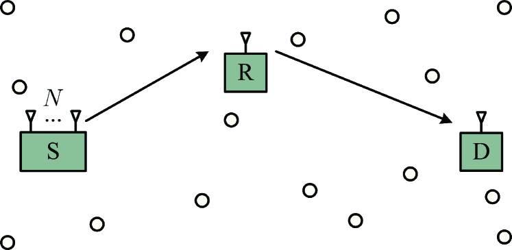
Figure 1: Illustration of a relay wiretap channel with spatially random eavesdroppers.

II-A Transmission Scheme

We now detail the proposed transmission scheme. The proposed scheme utilizes two time slots. In the first time slot, the source transmits information signals together with AN signals to the relay. In this time slot, the transmitted signals from the source are overheard by the eavesdroppers. The role of the AN signals is to confuse the eavesdroppers. In the second time slot, we assume that the source is silent. While it is clear that this will lead to a sub-optimal solution, such an assumption does allow for analytical tractability in a special case. Removing this assumption means more power can be added to the signal in the first time slot. Our other work [29], in which we consider multiple antennae at all nodes, quantifies the advantage of adding source noise in the second time slot. We also assume the relay transmits the received signals to the destination using the DF protocol. In this time slot, the broadcast signals are also overheard by the eavesdroppers. We assume that all the channels are subject to independent and identically distributed Rayleigh fading. We also assume a quasi-static block fading environment in which all the channel coefficients remain the same within one time slot. We denote $\mathbf{h}_{sr}$ as the $1\times N$ channel vector from the source to the relay and denote $h_{rd}$ as the channel coefficient from the relay to the destination.

We now express the transmitted and received signals in two time slots separately. In the first time slot, the transmitted signal at the source is given by

$$\mathbf{x}_{\text{S}}=\mathbf{W}\mathbf{t},$$ (1)

where $\mathbf{W}$ denotes the $N\times N$ beamforming matrix at the source and $\mathbf{t}$ denotes the combination of the information signal and the AN signal. To perform a such transmission, we first design $\mathbf{W}$ as

$$\mathbf{W}=\begin{bmatrix}\mathbf{w}_{\text{S}}&\mathbf{W}_{\text{AN}}\end{bmatrix},$$ (2)

where $\mathbf{w}_{\text{S}}$ is used to transmit the information signal and $\mathbf{W}_{\text{AN}}$ is used to transmit the AN signal. The aim of $\mathbf{W}$ is to degrade the quality of the received signals at the eavesdroppers. By transmitting AN signals into the null space of $\mathbf{h}_{sr}$ through $\mathbf{W}$, the source ensures that the quality of the received signals at the relay is free from AN interference. In designing $\mathbf{W}$, we choose $\mathbf{w}_{\text{S}}$ as the eigenvector corresponding to the largest eigenvalue of $\mathbf{h}_{sr}^{H}\mathbf{h}_{sr}$. We then choose $\mathbf{W}_{\text{AN}}$ as the remaining $N-1$ eigenvectors of $\mathbf{h}_{sr}^{H}\mathbf{h}_{sr}$. Such a design ensures that $\mathbf{W}$ is a unitary matrix. We then design $\mathbf{t}$ as

$$\mathbf{t}=\begin{bmatrix}t_{\text{S}}\\ \mathbf{t}_{\text{AN}}\end{bmatrix},$$ (3)

where $t_{\text{S}}$ denotes the information signal and $\mathbf{t}_{\text{AN}}$ is an $\left(N-1\right)\times 1$ vector of the AN signal. We define $\beta$, $0<\beta\leq 1$, as the fraction of the power allocated to the information signal. As such, we obtain $\mathbb{E}\left[|t_{\text{S}}|^{2}\right]=\beta$ and $\mathbb{E}\left[\mathbf{t}_{\text{AN}}\mathbf{t}_{\text{AN}}^{H}\right]=\frac{1-\beta}{N-1}\mathbf{I}_{N-1}$, where $\mathbb{E}\left[\cdot\right]$ is expectation and $\mathbf{I}_{m}$ is the $m\times{m}$ identity matrix. Moreover, we confirm that $\mathbb{E}\left[\mathbf{x}_{\text{S}}\mathbf{x}_{\text{S}}^{H}\right]=\mathbf{I}_{N}$. Based on (1), (2), and (3), the received signal at the relay in the first time slot is expressed as

$$y_{r}=\sqrt{P_{s}d_{sr}^{-\eta}}\mathbf{h}_{sr}\mathbf{w}_{\text{S}}t_{\text{S}}+n_{r},$$ (4)

where $P_{s}$ denotes the transmit power at the source, and $n_{r}$ denotes the thermal noise at the relay, which is assumed to be a zero mean complex Gaussian random variable with variance $\sigma_{r}^{2}$, i.e., $n_{r}\sim\mathcal{CN}\left(0,\sigma_{r}^{2}\right)$.

We next express the received signal at a typical eavesdropper located at $i$, $i\in\Phi$, in the first time slot as

$$y_{i}^{(1)}=\sqrt{P_{s}d_{si}^{-\eta}}\mathbf{h}_{si}\mathbf{w}_{\text{S}}t_{\text{S}}+\sqrt{P_{s}d_{si}^{-\eta}}\mathbf{h}_{si}\mathbf{W}_{\text{AN}}\mathbf{t}_{\text{AN}}+n_{i1},$$ (5)

where $\mathbf{h}_{si}$ denotes the $1\times N$ channel vector from the source to the typical eavesdropper located at $i$, $d_{si}$ denotes the distance between the source and the typical eavesdropper located at $i$, and $n_{i1}$ denotes the thermal noise at the typical eavesdropper located at $i$, which is assumed to be a zero mean complex Gaussian random variable with variance $\sigma_{i1}^{2}$, i.e., $n_{i1}\sim\mathcal{CN}\left(0,\sigma_{i1}^{2}\right)$.

In the second time slot, the relay adopts the DF protocol to forward signals to the destination. Specifically, the relay first decodes the transmitted signals from the source and then broadcasts them after re-encoding. Therefore, we express the received signal at the destination as

$$y_{d}=\sqrt{P_{r}d_{rd}^{-\eta}}h_{rd}x_{\text{R}}+n_{d},$$ (6)

where $P_{r}$ denotes the transmit power at the relay, $h_{rd}$ denotes the channel coefficient from the relay to the destination, $x_{\text{R}}$ denotes the transmitted signal of the relay with $\mathbb{E}\left[\|x_{\text{R}}\|^{2}\right]=1$, and $n_{d}$ denotes the thermal noise at the destination, which is assumed to be a zero mean complex random variable with variance $\sigma_{d}^{2}$, i.e., $n_{d}\sim\mathcal{CN}\left(0,\sigma_{d}^{2}\right)$.

We next express the received signal in the second time slot at the typical eavesdropper located at $i$ is expressed as

$$y_{i}^{(2)}=\sqrt{P_{r}d_{ri}^{-\eta}}h_{ri}x_{\text{R}}+n_{i2},$$ (7)

where $h_{ri}$ denotes the channel coefficient from the relay to the typical eavesdropper located at $i$, $d_{ri}$ denotes the distance between the relay and the typical eavesdropper located at $i$, and $n_{i2}$ denotes the thermal noise at the the typical eavesdropper located at $i$, which is assumed to be a zero mean complex random variable with variance $\sigma_{i2}^{2}$, i.e., $n_{i2}\sim\mathcal{CN}\left(0,\sigma_{i2}^{2}\right)$.

II-B Received SNRs

We express the instantaneous SNR at the destination as

$$\Gamma_{D}=\min\left\{\gamma_{sr},\gamma_{rd}\right\},$$ (8)

where $\gamma_{sr}=\frac{\beta{}P_{s}}{d_{sr}^{\eta}\sigma_{r}^{2}}\|\mathbf{h}_{sr}\|^{2}$ and $\gamma_{rd}=\frac{P_{r}}{d_{rd}^{\eta}\sigma_{d}^{2}}\|{h}_{rd}\|^{2}$. For the instantaneous SNR at the eavesdroppers, we assume that the eavesdroppers are non-colluding, which means that each eavesdropper decodes her own received signals from the source and the relay, without cooperating with other eavesdroppers. Thus, we express the instantaneous SNR at the eavesdroppers as

$$\Gamma_{E}=\max_{i\in\Phi}\left\{\max\left\{\gamma_{si},\gamma_{ri}\right\}\right\},$$ (9)

where

$$\gamma_{si}=\frac{\beta{}P_{s}d_{si}^{-\eta}\|\mathbf{h}_{si}\mathbf{w}_{\text{S}}\|^{2}}{\frac{1-\beta}{N-1}P_{s}d_{si}^{-\eta}\mathbf{h}_{si}\mathbf{W}_{\text{AN}}\mathbf{W}_{\text{AN}}^{H}\mathbf{h}_{si}^{H}+\sigma_{i1}^{2}}.$$ (10)

and $\gamma_{ri}=\frac{P_{r}}{d_{ri}^{\eta}\sigma_{i2}^{2}}\|h_{ri}\|^{2}$.

II-C Problem Formulation

In order to evaluate and optimize the secrecy performance achieved by our proposed scheme, we apply the performance metric proposed in [9], which is given by

$$T_{s}=\frac{1}{2}\left(R_{b}-R_{e}\right)\left(1-P_{to}\right),$$ (11)

where the factor $1/2$ is due to the two time slots used in the transmission, $\left(R_{b},R_{e}\right)$ denotes a parameter pair of the wiretap code used by the source, $R_{b}$ denotes the transmission rate of the wiretap code, $R_{e}$ denotes the cost of preventing the transmitted wiretap code from eavesdropping, and $P_{to}$ denotes the transmission outage probability ($P_{to}$ is defined as the probability that the instantaneous SNR at the destination is less than $\tau_{b}=2^{R_{b}}-1$). Mathematically, $P_{to}$ is formulated as

$$P_{to}={\Pr}\left(\Gamma_{D}\leq\tau_{b}\right).$$ (12)

Henceforth, we refer to $T_{s}$ as the secrecy throughput.

The goal of this work is to maximize the secrecy throughput of the relay wiretap channel with spatially random eavesdroppers under secrecy constraints. To achieve this goal, we formulate the design problem as

$$\max_{R_{b},R_{e},\beta} ~{}~{}T_{s},$$

$$s.t.~{}~{}P_{so}\leq\varphi,0\leq R_{e} \leq R_{b},0<\beta\leq 1,$$ (13)

where $P_{so}$ denotes the secrecy outage probability. $P_{so}$ is defined as the probability that $\Gamma_{E}$ is larger than $\tau_{e}=2^{R_{e}}-1$. Mathematically, $P_{so}$ is formulated as

$$P_{so}={\Pr}\left(\Gamma_{E}>\tau_{e}\right).$$ (14)

III Analysis and Optimization of Secrecy Performance

In this section, we first analyze the secrecy performance by deriving explicit expressions for the transmission probability and the secrecy outage probability, respectively. Based on these results we determine the optimal parameters, e.g., $R_{b}$, $R_{e}$, and $\beta$, that achieve the optimal secrecy performance of the relay wiretap channel. Notably, the determined optimal secrecy performance is independent of realizations of the main channel and the eavesdroppers’ channels.

III-A Transmission Outage Probability

In this subsection we focus on the transmission outage probability, $P_{to}$. We first obtain the cumulative distribution functions (CDFs) of $\gamma_{sr}$ and $\gamma_{rd}$ as

$$F_{\gamma_{sr}}\left(\gamma\right)=1-\exp\left(-\frac{\gamma}{\beta\overline{\gamma}_{sr}}\right)\sum_{n=0}^{N-1}\frac{1}{n!}\left(\frac{\gamma}{\beta\overline{\gamma}_{sr}}\right)^{n}$$ (15)

with $\overline{\gamma}_{sr}=P_{s}d_{sr}^{-\eta}\sigma_{r}^{-2}$, and

$$F_{\gamma_{rd}}\left(\gamma\right)=1-\exp\left(-\frac{\gamma}{\overline{\gamma}_{rd}}\right)$$ (16)

with $\overline{\gamma}_{rd}=P_{r}d_{rd}^{-\eta}\sigma_{d}^{-2}$. Based on (8), (15), and (16), we re-express the transmission outage probability in (12) as

$$P_{to}= {\Pr}\left(\min\left\{\gamma_{sr},\gamma_{rd}\right\}\leq\tau_{b}\right)$$

$$= 1-\left(1-F_{\gamma_{sr}}\left(\tau_{b}\right)\right)\left(1-F_{\gamma_{rd}}\left(\tau_{b}\right)\right)$$

$$= 1-\exp\left(-\left(\frac{1}{\beta\overline{\gamma}_{sr}}+\frac{1}{\overline{\gamma}_{rd}}\right)\tau_{b}\right)\sum_{n=0}^{N-1}\frac{1}{n!}\left(\frac{\tau_{b}}{\beta\overline{\gamma}_{sr}}\right)^{n}.$$ (17)

III-B Secrecy Outage Probability

We now focus on the secrecy outage probability, $P_{so}$. To derive $P_{so}$, we first express the CDFs of $\gamma_{si}$ and $\gamma_{ri}$ as

$$F_{\gamma_{si}}\left(\gamma\right)=1-\left(1+\frac{\left(1-\beta\right)\gamma}{\beta\left(N-1\right)}\right)^{-\left(N-1\right)}\exp\left(-\frac{\gamma}{\beta\overline{\gamma}_{si}}\right)$$ (18)

with $\overline{\gamma}_{si}=P_{s}d_{si}^{-\eta}\sigma_{i1}^{-2}$, and

$$F_{\gamma_{ri}}\left(\gamma\right)=1-\exp\left(-\frac{\gamma}{\overline{\gamma}_{ri}}\right)$$ (19)

with $\overline{\gamma}_{ri}=P_{r}d_{ri}^{-\eta}\sigma_{i2}^{-2}$. Based on (9), (18) and (19), we present the secrecy outage probability in the following theorem.

Theorem 1

The secrecy outage of the relay wiretap channel is derived as

$$P_{so}=1-\exp\left(-2\lambda\left(\mathcal{J}_{1}+\mathcal{J}_{2}-\mathcal{J}_{3}\right)\right),$$ (20)

where

$$\mathcal{J}_{1}= \frac{\pi}{\eta}\left(\frac{\beta P_{s}}{\tau_{e}\sigma_{i1}^{2}}\right)^{\frac{2}{\eta}}\left(1+\frac{\left(1-\beta\right)\tau_{e}}{\beta\left(N-1\right)}\right)^{-\left(N-1\right)}\Gamma\left(\frac{2}{\eta}\right),$$ (21)

$$\mathcal{J}_{2}=\int_{0}^{\infty}\int_{0}^{\pi}d_{si}\exp\left(-\psi\left(\theta\right)\right)dd_{si}d\theta,$$ (22)

$$\mathcal{J}_{3}= \left(1+\frac{\left(1-\beta\right)\tau_{e}}{\beta\left(N-1\right)}\right)^{-\left(N-1\right)}$$

$$\times\int_{0}^{\infty}\int_{0}^{\pi}d_{si}\exp\left(-\frac{\tau_{e}\sigma_{i1}^{2}}{\beta{}P_{s}}d_{si}^{\eta}\right)\exp\left(-\psi\left(\theta\right)\right)dd_{si}d\theta,$$ (23)

and $\psi\left(\theta\right)=\frac{\tau_{e}\sigma_{i2}^{2}}{P_{r}}\left(d_{sr}^{2}+d_{si}^{2}-2d_{sr}d_{si}\cos\theta\right)^{\frac{\eta}{2}}$.

Proof:

See Appendix A. ∎

We find that (20) provides an easy-to-compute expression for the secrecy outage probability. Despite that $\mathcal{J}_{2}$ and $\mathcal{J}_{3}$ for general $\eta$ can not be obtained in closed-form, they can be easily evaluated since only a double integral is involved in $\mathcal{J}_{2}$ and $\mathcal{J}_{3}$.

We next present simplified closed-form expressions for the special case where $\eta=2$. For this special case, we first simplify $\mathcal{J}_{2}$, which yields a closed-form expression given by (III-B) (next page),

$$\mathcal{J}_{2}= \exp\left(-\frac{\tau_{e}\sigma_{i2}^{2}}{P_{r}}d_{sr}^{2}\right)\int_{0}^{\infty}d_{si}\exp\left(-\frac{\tau_{e}\sigma_{i2}^{2}}{P_{r}}d_{si}^{2}\right)\int_{0}^{\pi}\exp\left(\frac{2\tau_{e}\sigma_{i2}^{2}}{P_{r}}d_{sr}d_{si}\cos\theta\right)d\theta dd_{si}$$

$$\overset{(a)}{=} \pi\exp\left(-\frac{\tau_{e}\sigma_{i2}^{2}}{P_{r}}d_{sr}^{2}\right)\int_{0}^{\infty}d_{si}\exp\left(-\frac{\tau_{e}\sigma_{i2}^{2}}{P_{r}}d_{si}^{2}\right)I_{0}\left(\frac{2\tau_{e}\sigma_{i2}^{2}}{P_{r}}d_{sr}d_{si}\right)dd_{si}$$

$$\overset{(b)}{=} \pi\exp\left(-\frac{\tau_{e}\sigma_{i2}^{2}}{P_{r}}d_{sr}^{2}\right)\int_{0}^{\infty}d_{si}\exp\left(-\frac{\tau_{e}\sigma_{i2}^{2}}{P_{r}}d_{si}^{2}\right)\sum_{k=0}^{\infty}\frac{1}{\left(k!\right)^{2}}\left(\frac{\tau_{e}\sigma_{i2}^{2}}{P_{r}}d_{sr}d_{si}\right)^{2k}dd_{si}$$

$$\overset{(c)}{=} \frac{\pi P_{r}}{2\tau_{e}\sigma_{i2}^{2}}\exp\left(-\frac{\tau_{e}\sigma_{i2}^{2}}{P_{r}}d_{sr}^{2}\right)\sum_{k=0}^{\infty}\frac{1}{\left(k!\right)^{2}}\left(\frac{\tau_{e}\sigma_{i2}^{2}}{P_{r}}d_{sr}^{2}\right)^{k}\Gamma\left(k+1\right)$$

$$\overset{(d)}{=} \frac{\pi P_{r}}{2\tau_{e}\sigma_{i2}^{2}}.$$ (24)

 

where $(a)$ follows by applying the expression of the zero-order modified Bessel function $I_{0}(z)$, $(b)$ follows by applying the series representation of $I_{0}(z)$, $(c)$ follows by using $t=\frac{\tau_{e}\sigma_{i2}^{2}}{P_{r}}d_{si}^{2}$ and noting that

$$\int_{0}^{\infty}t^{k}\exp\left(-t\right)dt=\Gamma\left(k+1\right),$$ (25)

and $(d)$ follows by applying the series expression representation of the exponential function. Similarly, for the special case where $\eta=2$, we simplify $\mathcal{J}_{3}$, which yields a closed-form expression given by (III-B) (next page). The simplified expressions in (III-B) and (III-B) offer us a computationally efficient way to calculate the secrecy outage probability for the special case where $\eta=2$.

$$\mathcal{J}_{3}= \left(1+\frac{\left(1-\beta\right)\tau_{e}}{\beta\left(N-1\right)}\right)^{-\left(N-1\right)}\!\!\exp\!\left(\!-\frac{\tau_{e}\sigma_{i2}^{2}}{P_{r}}d_{sr}^{2}\!\right)\!\int_{0}^{\infty}\!d_{si}\exp\!\left(\!-\left(\frac{\tau_{e}\sigma_{i1}^{2}}{\beta P_{s}}+\frac{\tau_{e}\sigma_{i2}^{2}}{P_{r}}\right)d_{si}^{2}\!\right)\!\int_{0}^{\pi}\exp\left(\frac{2\tau_{e}\sigma_{i2}^{2}}{P_{r}}d_{sr}d_{si}\cos\theta\right)d\theta dd_{si}$$

$$= \frac{\pi\beta P_{s}P_{r}}{2\tau_{e}\left(\beta P_{s}\sigma_{i2}^{2}+P_{r}\sigma_{i1}^{2}\right)}\exp\left(-\frac{\tau_{e}\sigma_{i1}^{2}\sigma_{i2}^{2}}{\beta P_{s}\sigma_{i2}^{2}+P_{r}\sigma_{i1}^{2}}d_{sr}^{2}\right)\left(1+\frac{\left(1-\beta\right)\tau_{e}}{\beta\left(N-1\right)}\right)^{-\left(N-1\right)}.$$ (26)

 

III-C Throughput Optimization

In this subsection we determine the optimal parameters that maximize the secrecy throughput, $T_{s}$, for general $\eta$. Specifically, we first determine the optimal wiretap code rates pair, $\left(R_{b}^{\ast},R_{e}^{\ast}\right)$, that maximizes the secrecy throughput for a given power allocation factor $\beta$. We then determine the joint optimal power allocation factor and wiretap code rates, $\left(\beta^{\ast\circ},R_{b}^{\ast\circ},R_{e}^{\ast\circ}\right)$, that maximizes $T_{s}$.

III-C1 Optimal wiretap code rates pair for a given $\beta$

The optimal wiretap code rates pair, $\left(R_{b}^{\ast},R_{e}^{\ast}\right)$, that maximizes $T_{s}$ for a given $\beta$ is determined as

$$\left(R_{b}^{\ast},R_{e}^{\ast}\right)=\operatorname*{argmax}~{}T_{s},$$

$$s.t.~{}~{}P_{so}\leq\varphi,0\leq R_{e}\leq R_{b}.$$ (27)

Taking the first-order derivative of $P_{so}$ with respect to $R_{e}$, we confirm that $\partial P_{so}/\partial R_{e}<0$, which states that $P_{so}$ monotonically decreases as $R_{e}$ increases. As such, the value of $R_{e}^{\ast}$ satisfying (III-C1) is the value of $R_{e}^{\ast}$ that satisfies the secrecy outage probability constraint, i.e., $P_{so}\left(R_{e}^{\ast}\right)=\varphi$. We then confirm that $\partial T_{s}/\partial R_{b}$ is first positive then negative as $R_{b}$ increases. This demonstrates that the value of $R_{b}^{\ast}$ satisfying (III-C1) is unique. Although a closed-form solution for $\left(R_{b}^{\ast},R_{e}^{\ast}\right)$ is mathematically intractable, we are able to determine the values of $\left(R_{b}^{\ast},R_{e}^{\ast}\right)$ numerically. Accordingly, the maximal secrecy throughput based on the values of $\left(R_{b}^{\ast},R_{e}^{\ast}\right)$ for a given $\beta$ is defined as $T_{s}^{\ast}$.

III-C2 Joint optimization of $\beta$, $R_{b}$, and $R_{e}$

The joint optimal power allocation factor and wiretap code rates which maximizes $T_{s}$ in (11), $\left(\beta^{\ast\circ},R_{b}^{\ast\circ},R_{e}^{\ast\circ}\right)$, is determined as

$$\left(\beta^{\ast\circ},R_{b}^{\ast\circ},R_{e}^{\ast\circ}\right) =\operatorname*{argmax}~{}T_{s},$$

$$s.t.~{}~{}P_{so}\leq\varphi,~{}0\leq R_{e} \leq R_{b},~{}0<\beta\leq 1.$$ (28)

Using (III-A) and (20), we are able to solve (III-C2) numerically. Specifically, we first determine the value of $\left(R_{b}^{\ast},R_{e}^{\ast}\right)$ using (III-C1) for each value of $\beta$. This leads to the secrecy throughput with $\left(R_{b}^{\ast},R_{e}^{\ast}\right)$, denoted by $T_{s}^{\ast}=\frac{1}{2}\left(R_{b}^{\ast}-R_{e}^{\ast}\right)\left(1-P_{to}\right)$. We then determine the value of $\beta$ that maximizes $T_{s}^{\ast}$, denoted by $\beta^{\ast\circ}$. Accordingly, the value of $\left(R_{b}^{\ast},R_{e}^{\ast}\right)$ associated with $\beta^{\ast\circ}$ is determined as $\left(R_{b}^{\ast\circ},R_{e}^{\ast\circ}\right)$. Finally, the maximal secrecy throughput based on the values of $\beta^{\ast\circ}$, $R_{b}^{\ast\circ}$, and $R_{e}^{\ast\circ}$ is defined as $T_{s}^{\ast\circ}$.

IV Numerical Results

In this section we present numerical results to validate our analysis of the outage probabilities and examine the benefits of the proposed scheme. For illustrative purpose, throughout this section we concentrate on the practical example of a highly shadowed urban area with $\eta=4$. In addition, we adopt $\lambda d_{sr}^{2}=\lambda d_{rd}^{2}=1$.

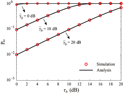
Figure 2: $P_{to}$ versus $\tau_{b}$ for different values of $\overline{\gamma}_{b}$ with $\eta=4$, $N=4$, and $\beta=0.5$.

We first verify the accuracy of the transmission outage probability and the secrecy outage probability using Monte Carlo simulations. In Fig. 2, we plot $P_{to}$ versus $\tau_{b}$ for different values of $\overline{\gamma}_{b}$ with $N=4$ and $\beta=0.5$. In this figure, we consider $\overline{\gamma}_{sr}=\overline{\gamma}_{rd}=\overline{\gamma}_{b}$. We first see that the analytical curves, generated from (III-A), precisely match the simulation points, which demonstrates the correctness of our expression for $P_{to}$ in (III-A). Second, we see that $P_{to}$ increases monotonically as $\tau_{b}$ increases for a given $\overline{\gamma}_{b}$, which implies that the transmission outage probability increases when the transmission rate of the wiretap code increases. We further see that $P_{to}$ decreases as $\overline{\gamma}_{b}$ increases for a given $\tau_{b}$. This reveals that the transmission outage probability reduces when the source and the relay use more power to transmit under a fixed $\tau_{b}$.

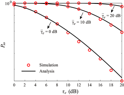
Figure 3: $P_{so}$ versus $\tau_{e}$ for different values of $\overline{\gamma}_{e}$ with $\eta=4$, $N=4$, and $\beta=0.5$.

In Fig. 3, we plot $P_{so}$ versus $\tau_{e}$ for different values of $\overline{\gamma}_{e}$ with $N=4$ and $\beta=0.5$. In this figure we consider $\overline{\gamma}_{sr}{\sigma_{r}^{2}}/{\sigma_{i1}^{2}}=\overline{\gamma}_{rd}{\sigma_{d}^{2}}/{\sigma_{i2}^{2}}=\overline{\gamma}_{e}$. We see an excellent match between the analytical curves generated from (20) and the simulation points, demonstrating the correctness of our expression for $P_{so}$ in (20). We then see that $P_{so}$ decreases monotonically as $\tau_{e}$ increases for a given $\overline{\gamma}_{e}$, which shows that the secrecy outage probability decreases when the redundancy rate of the wiretap code increases. We further observe that $P_{so}$ increases as $\overline{\gamma}_{e}$ increases. This is due to the fact the eavesdroppers receive signals from both the source and the relay. It follows that increasing the transmit power at the source and the relay leads to an improved received SNR at the eavesdroppers.

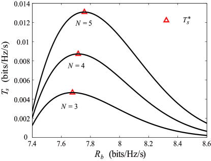
Figure 4: $T_{s}$ versus $R_{b}$ for different values of $N$ with $\eta=4$, $\beta=0.5$, $\varphi=0.4$, $\overline{\gamma}_{b}=20$ dB, and $\overline{\gamma}_{b}/\overline{\gamma}_{e}=20$.

We now examine the impact of the system parameters $R_{b}$ and $\beta$ on the secrecy throughput. In Fig. 4, we plot $T_{s}$ versus $R_{b}$ for different values of $N$ with a fixed $\beta$ and the optimal $R_{e}$. We first observe that there exists a unique $R_{b}^{\ast}$ that maximizes $T_{s}$ for a given $\beta$. We also observe that the maximal $T_{s}$ for a given $\beta$, i.e., $T_{s}^{\ast}$, increases as $N$ increases. This shows that adding extra transmit antennas at the source significantly enhances the secrecy performance of the relay wiretap channel.

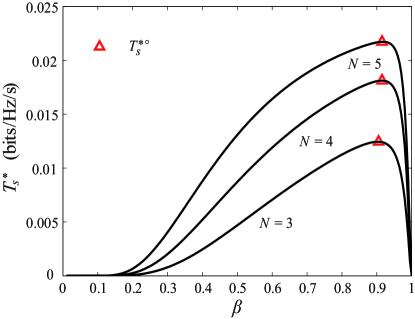
Figure 5: $T_{s}^{\ast}$ versus $\beta$ for different values of $N$ with $\eta=4$, $\varphi=0.4$, $\overline{\gamma}_{b}=20$ dB, and $\overline{\gamma}_{b}/\overline{\gamma}_{e}=20$.

In Fig. 5, we plot $T_{s}^{\ast}$ versus $\beta$ for different values of $N$. For each point of $T_{s}^{\ast}$, we choose the $\left(R_{b}^{\ast},R_{e}^{\ast}\right)$ pair that maximizes $T_{s}$ for the corresponding $\beta$. We first observe that there exists a unique $\beta^{\ast\circ}$ that maximizes $T_{s}^{\ast}$. We then observe that the value of $\beta^{\ast\circ}$ that maximizes $T_{s}^{\ast}$ is around $0.9$, which demonstrates that the secrecy throughput is improved if approximately 10% of the total transmit power at the source is allocated to AN signals. We also observe that the maximal $T_{s}^{\ast}$, i.e., $T_{s}^{\ast\circ}$, increases as $N$ increases. Furthermore, we observe that the value of $\beta^{\ast\circ}$ slightly decreases as $N$ increases, which shows that in order to maintain the optimal secrecy throughput, the power allocated to AN must increase as the source antenna number increases.

V Conclusion

In this work we proposed a secure transmission scheme for a relay wiretap channel, in which an $N$-antenna source transmits both information signals and AN signals in the presence of multiple spatially random single-antenna eavesdroppers. Conditioned on the use of a decode-and-forward protocol at the relay, we determined the optimal parameters $\left(\beta^{\ast\circ},R_{b}^{\ast\circ},R_{e}^{\ast\circ}\right)$ that maximizes the secrecy throughput, based on our derived expressions for the transmission outage probability and the secrecy outage probability. In addition, we examined the impact of $N$ on the secrecy throughput, showing how the maximal secrecy throughput increases with $N$. The work reported here provides valuable insights into the design of new physical layer security schemes in which the locations of the eavesdroppers are randomly distributed and not known at the source.

Appendix A Proof of Theorem 1

According to (9), (18) and (19), we re-express (14) as

$$P_{so} =1-{\Pr}\left\{\Gamma_{E}\leq\tau_{e}\right\}$$

$$=1-{\Pr}\left\{\max_{i\in\Phi}\left\{\max\left\{\gamma_{si},\gamma_{ri}\right\}\right\}\leq\tau_{e}\right\}$$

$$=1-\mathbb{E}_{\Phi}\left[\prod_{i\in\Phi}{\Pr}\left\{\max\left\{\gamma_{si},\gamma_{ri}\right\}\leq\tau_{e}\right\}\right]$$

$$=1-\mathbb{E}_{\Phi}\left[\prod_{i\in\Phi}\left(1-\left(1+\frac{\left(1-\beta\right)\tau_{e}}{\beta\left(N-1\right)}\right)^{-\left(N-1\right)}\right.\right.$$

$$~{}~{}\left.\left.\times\exp\left(-\frac{\tau_{e}}{\beta\overline{\gamma}_{si}}\right)\right)\left(1-\exp\left(-\frac{\tau_{e}}{\overline{\gamma}_{ri}}\right)\right)\right]$$

$$\overset{(a)}{=}1-\exp\left(-2\lambda\left(\mathcal{J}_{1}+\mathcal{J}_{2}-\mathcal{J}_{3}\right)\right).$$ (29)

where

$$\mathcal{J}_{1}= \int_{0}^{\infty}\int_{0}^{\pi}d_{si}\left(\left(1+\frac{\left(1-\beta\right)\tau_{e}}{\beta\left(N-1\right)}\right)^{-\left(N-1\right)}\right.$$

$$\left.\hskip 56.9055pt\times\exp\left(-\frac{\tau_{e}\sigma_{i1}^{2}}{\beta P_{s}}d_{si}^{\eta}\right)\right)dd_{si}d\theta,$$ (30)

$$\mathcal{J}_{2}=\int_{0}^{\infty}\int_{0}^{\pi}d_{si}\exp\left(-\frac{\tau_{e}\sigma_{i2}^{2}}{P_{r}}d_{ri}^{\eta}\right)dd_{si}d\theta,$$ (31)

and

$$\mathcal{J}_{3}= \int_{0}^{\infty}\int_{0}^{\pi}d_{si}\left(1+\frac{\left(1-\beta\right)\tau_{e}}{\beta\left(N-1\right)}\right)^{-\left(N-1\right)}$$

$$\hskip 28.45274pt\times\exp\left(-\frac{\tau_{e}\sigma_{i1}^{2}}{\beta P_{s}}d_{si}^{\eta}-\frac{\tau_{e}\sigma_{i2}^{2}}{P_{r}}d_{ri}^{\eta}\right)dd_{si}d\theta,$$ (32)

and $(a)$ follows by applying the probability generating functional (PGFL) for the PPP $\Phi$, given by [30]

$$\mathbb{E}_{\Phi}\left[\prod_{x\in\Phi}f\left(x\right)\right]=\exp\left\{-\int_{\mathbb{R}^{2}}\left[1-f\left(x\right)\right]\lambda dx\right\},$$ (33)

and by changing to polar coordinates.

To proceed, we first derive $\mathcal{J}_{1}$ as

$$\mathcal{J}_{1} =\pi\left(1+\frac{\left(1-\beta\right)\tau_{e}}{\beta\left(N-1\right)}\right)^{-\left(N-1\right)}$$

$$\hskip 56.9055pt\times\int_{0}^{\infty}d_{si}\exp\left(-\frac{\tau_{e}\sigma_{i1}^{2}}{\beta P_{s}}d_{si}^{\eta}\right)dd_{si}$$

$$\overset{(b)}{=}\frac{\pi}{2}\left(1+\frac{\left(1-\beta\right)\tau_{e}}{\beta\left(N-1\right)}\right)^{-\left(N-1\right)}$$

$$\hskip 56.9055pt\times\int_{0}^{\infty}\exp\left(-\frac{\tau_{e}\sigma_{i1}^{2}}{\beta P_{s}}u^{\frac{\eta}{2}}\right)du$$

$$\overset{(c)}{=}\frac{\pi}{\eta}\left(\frac{\beta P_{s}}{\tau_{e}\sigma_{i1}^{2}}\right)^{\frac{2}{\eta}}\left(1+\frac{\left(1-\beta\right)\tau_{e}}{\beta\left(N-1\right)}\right)^{-\left(N-1\right)}$$

$$\hskip 56.9055pt\times\int_{0}^{\infty}\exp\left(-t\right)t^{\frac{2}{\eta}-1}dt$$

$$\overset{(d)}{=}\frac{\pi}{\eta}\left(\frac{\beta P_{s}}{\tau_{e}\sigma_{i1}^{2}}\right)^{\frac{2}{\eta}}\left(1+\frac{\left(1-\beta\right)\tau_{e}}{\beta\left(N-1\right)}\right)^{-\left(N-1\right)}\Gamma\left(\frac{2}{\eta}\right),$$ (34)

where in $(b)$ we have used $u=d_{si}^{2}$, in $(c)$ we have used $t=\frac{\tau_{e}\sigma_{i1}^{2}}{\beta P_{s}}u^{\frac{\eta}{2}}$, and $(d)$ follows from the definition of the gamma function. We then derive $\mathcal{J}_{2}$ as

$$\mathcal{J}_{2}$$

$$= \int_{0}^{\infty}\!\!\!\!\int_{0}^{\pi}\!\!\!d_{si}\exp\!\left(\!\!-\frac{\tau_{e}\sigma_{i2}^{2}}{P_{r}}\!\left(d_{sr}^{2}+d_{si}^{2}\!-\!2d_{sr}d_{si}\cos\theta\right)^{\frac{\eta}{2}}\!\right)\!dd_{si}d\theta.$$ (35)

We further derive $\mathcal{J}_{3}$ as

$$\mathcal{J}_{3}$$

$$= \left(1+\frac{\left(1-\beta\right)\tau_{e}}{\beta\left(N-1\right)}\right)^{-\left(N-1\right)}\int_{0}^{\infty}\int_{0}^{\pi}d_{si}\exp\left(-\frac{\tau_{e}\sigma_{i1}^{2}}{\beta P_{s}}d_{si}^{\eta}\right)$$

$$\times\exp\!\left(\!-\frac{\tau_{e}\sigma_{i2}^{2}}{P_{r}}\left(d_{sr}^{2}\!+\!d_{si}^{2}\!-\!2d_{sr}d_{si}\cos\theta\right)^{\frac{\eta}{2}}\!\right)\!dd_{si}d\theta.$$ (36)

Substituting (A), (A), and (A) into (A), we obtain the desired result in (20), which completes the proof.

References

- [1] Y.-W. P. Hong, P.-C. Lan, and C.-C. J. Kuo, “Enhancing physical-layer secrecy in multiantenna wireless systems: An overview of signal processing approaches,” IEEE Signal Process. Mag., vol. 30, no. 5, pp. 29–40, Sep. 2013.
- [2] N. Yang, L. Wang, G. Geraci, M. Elkashlan, J. Yuan, and M. Di Renzo,“Safeguarding 5G wireless communication networks using physical layer security,” IEEE Commun. Mag., accepted to appear.
- [3] A. Wyner, “The wire-tap channel,” Bell Syst. Tech. J., vol. 54, no. 8, pp. 1355–1387, Oct. 1975.
- [4] A. Khisti and G. W. Wornell, “Secure transmission with multiple antennas I: The MISOME wiretap channel,” IEEE Trans. Inf. Theory, vol. 56, no. 6, pp. 3088–3104, Jul. 2010.
- [5] A. Khisti and G. W. Wornell, “Secure transmission with multiple antennas II: The MIMOME wiretap channel,” IEEE Trans. Inf. Theory, vol. 56, no. 11, pp. 5515–5532, Nov. 2010.
- [6] C. Liu, G. Geraci, N. Yang, J. Yuan, and R. Malaney, ”Beamforming for MIMO Gaussian channels with imperfect channel state information,” in Proc. IEEE GlobeCOM 2013, Atlanta, USA, Dec. 2013.
- [7] C. Liu, N. Yang, G. Geraci, J. Yuan, and R. Malaney, “Secrecy in MIMOME wiretap channels: Beamforming with imperfect CSI,” in Proc. IEEE ICC 2014, Sydney, Australia, Jun. 2014.
- [8] C. Liu, N. Yang, S. Yan, J. Yuan, and R. Malaney,“Secure adaptive transmission in two-way relay wiretap channels,” in Proc. IEEE/CIC ICCC 2014, Shanghai, China, Oct. 2014.
- [9] X. Zhou and M. R. McKay, B. Maham, and A. Hjørungnes, “Rethinking the secrecy outage formulation: A secure transmission design perspective,” IEEE Commun. Lett., vol. 15, no. 3, pp. 302–304, Mar. 2011.
- [10] X. Zhang, X. Zhou, and M. R. McKay, “On the design of artificial-noise-aided secure multi-antenna transmission in slow fading channels,” IEEE Trans. Veh. Technol., vol. 62, no. 5, pp. 2170–2181, Jun. 2013.
- [11] N. Yang, P. L. Yeoh, M. Elkashlan, R. Schober, and I. B. Collings, “Transmit antenna selection for security enhancement in MIMO wiretap channels,” IEEE Trans. Commun., vol. 61, no. 1, pp. 144–154, Jan. 2013.
- [12] N. Yang, H. A. Suraweera, I. B. Collings, and C. Yuen, “Physical layer security of TAS/MRC with antenna correlation,” IEEE Trans. Inf. Forensic Security, vol. 8, no. 1, pp. 254–259, Jan. 2013.
- [13] N. Yang, P. L. Yeoh, M. Elkashlan, R. Schober, and J. Yuan, “MIMO wiretap channels: A secure transmission using transmit antenna selection and receive generalized selection combining,” IEEE Commun. Lett., vol. 17, no. 9, pp. 1754–1757, Sep. 2013.
- [14] N. Yang, G. Geraci, J. Yuan, and R. Malaney, “Confidential broadcasting via linear precoding in non-homogeneous MIMO multiuser networks,” IEEE Trans. Commun., vol. 62, no. 7, pp. 2515–2530, July 2014.
- [15] S. Yan, N. Yang, R. Malaney, and J. Yuan, “Transmit antenna selection with Alamouti coding and power allocation in MIMO wiretap channels,” IEEE Trans. Wireless Commun., vol. 13, no. 3, pp. 1656–1667, Mar. 2014.
- [16] X. Zhou, R. K. Ganti, J. G. Andrews, and A. Hjørungnes, “On the throughput cost of physical layer security in decentralized wireless networks,” IEEE Trans. Wireless Commun., vol. 10, no. 8, pp. 2764–2775, Aug. 2011.
- [17] H. Wang, X. Zhou, and M. C. Reed, “Physical layer security in cellular networks: A stochastic geometry approach,” IEEE Trans. Wireless Commun., vol. 12, no. 6, pp. 2776–2787, Jun. 2013.
- [18] G. Geraci, S. Singh, J. G. Andrews, J. Yuan, and I. B. Collings, “Secrecy rates in broadcast channels with confidential messages and external eavesdroppers,”IEEE Trans. Wireless Commun., vol. 13, no. 5, pp. 2931–2943, May 2014.
- [19] G. Geraci, H. S. Dhillon, J. G. Andrews, J. Yuan, and I. B. Collings, “Physical layer security in downlink multi-antenna cellular networks,” IEEE Trans. Commun., vol. 62, no. 6, pp. 2006–2021, Jun. 2014.
- [20] J. N. Laneman, D. N. C. Tse, and G. W. Wornell, “Cooperative diversity in wireless networks: Efficient protocols and outage behavior,” IEEE Trans. Inf. Theory, vol. 50, pp. 3062–3080, Dec. 2004.
- [21] R. Bassily, E. Ekrem, X. He, E. Tekin, J. Xie, M. R. Bloch, S. Ulukus, and A. Yener, “Cooperative security at the physical layer: A summary of recent advances,” IEEE Signal Process. Mag., vol. 30, no. 5, pp. 16–28, Sep. 2013.
- [22] L. Dong, Z. Han, A. Petropulu, and H. V. Poor, “Improving wireless physical layer security via cooperating relays,” IEEE Trans. Signal Process., vol. 58, no. 3, pp. 1875–1888, Mar. 2010.
- [23] X. Chen, C. Zhong, C. Yuen, and H.-H. Chen, “Multi-antenna relay aided wireless physical layer security,” IEEE Commun. Mag., accepted.
- [24] X. Chen, L. Lei, H. Zhang, and C. Yuen, “Large-scale MIMO relaying techniques for physical layer security: AF or DF?” IEEE Trans. Wireless Commun., accepted.
- [25] Y. Zou, X. Wang, and W. Shen, “Optimal relay selection for physical-layer security in cooperative wireless networks,” IEEE J. Sel. Areas Commun., vol. 31, no. 10, pp. 2099–2111, Oct. 2013.
- [26] J. Chen, L. Song, Z. Han, and B. Jiao, “Joint relay and jammer selection for secure two-way relay networks,” IEEE Trans. Inf. Foren. Sec., vol. 7, no. 1, pp. 310–320, Feb. 2012.
- [27] C. Liu, N. Yang, J. Yuan, and R. Malaney, “Location-based secure transmission for wiretap channels,” IEEE J. Sel. Areas Commun., vol. 33, no. 7, pp. 1458–1470, Jul. 2015.
- [28] S. Weber, J. G. Andrews, and N. Jindal, “An overview of the transmission capacity of wireless networks,” IEEE Trans. Commun., vol. 58, no. 12, pp. 3593–3604, Dec. 2010.
- [29] C. Liu, N. Yang, R. Malaney, and J. Yuan, “Artificial-noise-aided transmission in multi-antenna relay wiretap channels with spatially random eavesdroppers,” arXiv:1509.05486.
- [30] D. Stoyan, W. Kendall, and J. Mecke, Stochastic Geometry and its Applications, 2nd ed. John Wiley Sons Ltd., 1996.