An Automata Theoretic Approach to the Zero-One Law for Regular Languages: Algorithmic and Logical Aspects

Abstract

A zero-one language $L$ is a regular language whose asymptotic probability converges to either zero or one. In this case, we say that $L$ obeys the zero-one law. We prove that a regular language obeys the zero-one law if and only if its syntactic monoid has a zero element, by means of Eilenberg’s variety theoretic approach. Our proof gives an effective automata characterisation of the zero-one law for regular languages, and it leads to a linear time algorithm for testing whether a given regular language is zero-one. In addition, we discuss the logical aspects of the zero-one law for regular languages.

1 Introduction

Let $L$ be a regular language over a non-empty finite alphabet $A$. Recall that the counting function $\gamma_{n}(L)$ of $L$ counts the number of different words of length $n$ in $L$: $\gamma_{n}(L)=|L\cap A^{n}|$ where $A^{n}$ is the set of all words of length $n$ over $A$. The probability function $\mu_{n}(L)$ of $L$ is the fraction defined by

$$\mu_{n}(L)=\frac{\gamma_{n}(L)}{\gamma_{n}(A^{*})}=\frac{|L\cap A^{n}|}{|A^{n}|}.$$

The asymptotic probability $\mu(L)$ of $L$ is defined by $\mu(L)=\lim_{n\rightarrow\infty}\mu_{n}(L)$, if the limit exists. We can regard $\mu_{n}(L)$ as the probability that a randomly chosen word of length $n$ is in $L$, and $\mu(L)$ as its asymptotic probability. Here we introduce a new class of regular languages which is the main target of this paper.

Definition 1 (zero-one language).

A zero-one language $L$ is a regular language whose asymptotic probability $\mu(L)$ is either zero or one. In this case, we say that $L$ obeys the zero-one law. We denote by ${\cal Z\!\!O}$ the class of all regular zero-one languages.

As we will describe later (see Section 7), the notion of “zero-one law” defined here is a fundamental object in finite model theory.

Example 1.

We now consider a few examples.

• The set of all words $A^{*}$ over $A$ satisfies $\mu(A^{*})=1$, and its complement $\emptyset$ satisfies $\mu(\emptyset)=0$. These two languages obey the zero-one law.

• Consider $aA^{*}$ the set of all words which start with the letter $a$ in $A$. Then

  $$\mu_{n}(aA^{*})=\frac{|aA^{n-1}|}{|A^{n}|}=\frac{1}{|A|}.$$

  Hence, its limit $\mu((aA)^{*})$ is $1/|A|$ and $aA^{*}$ is zero-one if and only if $A$ is unary: $A=\{a\}$.

• Consider $(AA)^{*}$ the set of all words with even length. Then

  $$\mu_{n}((AA)^{*})=\begin{cases}1&\text{if}\;\;n\;\;\text{is even,}\\ 0&\text{if}\;\;n\;\;\text{is odd.}\end{cases}$$

  Hence, its limit $\mu((AA)^{*})$ does not exist.

Thus, for some regular language $L$, the asymptotic probability $\mu(L)$ is either zero or one, for some, like $L=aA^{*}$ where $|A|\geq 2$, $\mu(L)$ could be a real number between zero and one, and for some, like $L=(AA)^{*}$, it may not even exist. It is previously known that there exists a cubic time algorithm computing $\mu(L)$ for any regular language $L$ ([6], see Section 8).

Our results and contributions.  In this paper, we show that the following class of languages exactly captures the zero-one law for regular languages.

Definition 2 ([17]).

A language with zero is a regular language whose syntactic monoid has a zero element. We denote by ${\cal Z}$ the class of all regular languages with zero.

More precisely, we prove the following theorem, which states that ${\cal Z\!\!O}$ and ${\cal Z}$ are equivalent by means of a transparent condition of their automata: zero automata (Section 3) and quasi-zero automata (Section 6) which will be described later. The remarkable fact is that, ${\cal Z\!\!O}={\cal Z}$ holds even though these two notions seem completely different from each other; ${\cal Z\!\!O}$ is defined by the asymptotic behavior of its probability, ${\cal Z}$ is defined by the existence of a zero of its syntactic monoid.

Theorem 1.

Let $L$ be a regular language and ${\cal A}_{L}$ be the minimal automaton of L. Then the following four conditions are equivalent.

1. ${\cal A}_{L}$ is zero.

2. $L$ is with zero.

3. $L$ obeys the zero-one law.

4. $L$ is recognised by a quasi-zero automaton.

We will prove this theorem as a cyclic chain of implications: ${\color[rgb]{1,0,0}\scriptsize\ref{condition:za}⃝}\Rightarrow{\color[rgb]{1,0,0}\scriptsize\ref{condition:zero}⃝}\Rightarrow{\color[rgb]{1,0,0}\scriptsize\ref{condition:zeroone}⃝}\Rightarrow{\color[rgb]{1,0,0}\scriptsize\ref{condition:za}⃝}$, and ${\color[rgb]{1,0,0}\scriptsize\ref{condition:za}⃝}\Leftrightarrow{\color[rgb]{1,0,0}\scriptsize\ref{condition:quasi}⃝}$ independently. We should notice that the most difficult part of this proof is the implication ${\color[rgb]{1,0,0}\scriptsize\ref{condition:zeroone}⃝}\Rightarrow{\color[rgb]{1,0,0}\scriptsize\ref{condition:za}⃝}$, while the former part ${\color[rgb]{1,0,0}\scriptsize\ref{condition:za}⃝}\Rightarrow{\color[rgb]{1,0,0}\scriptsize\ref{condition:zero}⃝}\Rightarrow{\color[rgb]{1,0,0}\scriptsize\ref{condition:zeroone}⃝}$ is easy. The key points of the proof of this part are closure properties of ${\cal Z\!\!O}$ and Lemma 1, which comes from Eilenberg’s variety theorem. The automata characterisation ${\color[rgb]{1,0,0}\scriptsize\ref{condition:quasi}⃝}$ of Theorem 1 leads to a linear time algorithm for testing whether a given regular language is zero-one. In addition, our automata theoretic proof sheds new light on the relation between the zero-one law for regular languages and logical fragments over finite words.

Paper outline.  The remainder of this paper is organised as follows. In Section 2, we first give the necessary definitions and terminology for languages, monoids, and automata. Lemma 1 will be introduced in this section. For the sake of completeness we include the proof of Lemma 1. Section 3 provides a detailed exposition of the notion of zero automata. Our automata theoretic proof of Theorem 1 consists of three parts: (i) Check certain closure properties of ${\cal Z\!\!O}$ (Section 4), (ii) Apply Lemma 1 to prove the implication ${\color[rgb]{1,0,0}\scriptsize\ref{condition:zeroone}⃝}\Rightarrow{\color[rgb]{1,0,0}\scriptsize\ref{condition:za}⃝}$ (Section 5). (iii) Generalise the notion of zero automata, and prove ${\color[rgb]{1,0,0}\scriptsize\ref{condition:za}⃝}\Leftrightarrow{\color[rgb]{1,0,0}\scriptsize\ref{condition:quasi}⃝}$ (Section 6). In Section 6, we will give a linear time algorithm (Theorem 2). The logical aspects of our results are investigated in Section 7. Finally, we discuss some related works of our results and conclude this paper in Section 8. We try to keep all sections as self-contained as possible.

2 Preliminaries

In this paper, all considered automata are deterministic finite, complete and accessible. We refer the reader to the book by Sakarovitch [19] for background material.

Languages and monoids.  We denote by $A^{*}\;[A^{n}]$ the set of all words [of length $n$] over a nonempty finite alphabet $A$, and by $|w|$ the length of a word $w$ in $A^{*}$. The empty word is denoted by $\varepsilon$. That is, $A^{*}$ is the free monoid over $A$ with the neutral element $\varepsilon$. We can easily verify that

$$\mu_{n+k}(A^{k}L)=\frac{|A^{k}L\cap A^{n+k}|}{|A^{n+k}|}=\frac{|A^{k}(L\cap A^{n})|}{|A^{k}A^{n}|}=\frac{|L\cap A^{n}|}{|A^{n}|}=\mu_{n}(L)$$

holds for any language $L$ of $A^{*}$ and $k\geq 0$. It follows from what has been said that $\mu(A^{k}L)$ exists if and only if $\mu(L)$ exists and in that case they are equal $\mu(A^{k}L)=\mu(L)$. If two languages $L$ and $K$ of $A^{*}$ are mutually disjoint ($L\cap K=\emptyset$), then clearly $\mu(L\cup K)=\mu(L)+\mu(K)$ holds if both $\mu(L)$ and $\mu(K)$ exist. We say that $v$ is a factor of $w$ if, there exists $x,y$ in $A^{*}$ such that $w=xvy$. Let $L$ be a language of $A^{*}$ and let $u$ be a word of $A^{*}$. The left [right] quotient $u^{-1}L\;[Lu^{-1}]$ of $L$ by $u$ is defined by

$$u^{-1}L=\{v\in A^{*}\mid uv\in L\}\;\;\;\;\;\;\text{and}\;\;\;\;\;\;Lu^{-1}=\{v\in A^{*}\mid vu\in L\}.$$

We denote by $\overline{L}=A^{*}\setminus L$ the complement of $L$. The syntactic congruence of $L$ of $A^{*}$ is the relation $\sim_{L}$ defined on $A^{*}$ by $u\sim_{L}v$ if and only if, $xuy\in L\Leftrightarrow xvy\in L$ holds for all $x,y$ in $A^{*}$. The quotient $A^{*}/\sim_{L}$ is called the syntactic monoid of $L$ and the natural morphism $\phi_{L}:A^{*}\rightarrow A^{*}/\sim_{L}$ is called the syntactic morphism of $L$. If $M$ is a monoid, an element $\bm{0}$ in $M$ is said to be a zero if, $\bm{0}m=m\bm{0}=\bm{0}$ holds for all $m$ in $M$.

Automata and an important lemma.  An (complete deterministic finite) automaton over a finite alphabet $A$ is a quintuple ${\cal A}=\langle Q,A,\cdot,q_{0},F\rangle$ where

• $Q$ is a finite set of states;

• $\cdot:Q\times A\rightarrow Q$ is a transition function, which can be extended to a mapping $\cdot:Q\times A^{*}\rightarrow Q$ by $q\cdot\varepsilon=q$ and $q\cdot aw=(q\cdot a)\cdot w$ where $q\in Q,a\in A$ and $w\in A^{*}$;

• $q_{0}\in Q$ is an initial state, and $F\subseteq Q$ is a set of final states.

The language recognised by ${\cal A}$ is denoted by $L({\cal A})=\{w\in A^{*}\mid q_{0}\cdot w\in F\}$. We say that ${\cal A}$ recognises $L$ if $L=L({\cal A})$. It is a basic fact that, for any regular language $L$, there exists a unique automaton recognises $L$ which has the minimum number of states: the minimal automaton of $L$ and we denote it by ${\cal A}_{L}$. Each word $w$ in $A^{*}$ defines the transformation $w:q\mapsto q\cdot w$ on $Q$. The transition monoid of ${\cal A}$ is equal to the transformation monoid generated by the generators $A$. It is well known that the syntactic monoid of a regular language is equal to the transition monoid of its minimal automaton.

For any subset $P$ of $Q$, the past of $P$ is the language denoted by ${\sf{Past}}(P)$ and defined by

$${\sf{Past}}(P)=\{w\in A^{*}\mid q_{0}\cdot w\in P\}.$$

Dually, the future of a subset $P$ of $Q$ is the language denoted by ${\sf{Fut}}(P)$ and defined by

$${\sf{Fut}}(P)=\{w\in A^{*}\mid\exists p\in P,p\cdot w\in F\}.$$

It is well known that, an (accessible) automaton ${\cal A}$ is minimal if and only if the following condition

$$p=q\;\;\;\;\Leftrightarrow\;\;\;\;{\sf{Fut}}(p)={\sf{Fut}}(q)$$ (M)

holds for every pair of states $p,q$ in $Q$. Myhill-Nerode theorem states that every regular language has only a finite number of left and right quotients.

In Section 5, to prove Theorem 1, we will use the following technical but important lemma. For the sake of completeness we include the proof, which is essentially based on “Proof of Theorem 3.2 and 3.2s” in the book [8] by Eilenberg.

Lemma 1.

Let ${\cal A}_{L}=\langle Q,A,\cdot,q_{0},F\rangle$ be the minimal automaton of a language $L$. Then for any subset $P$ of $Q$, its past ${\sf{Past}}(P)$ can be expressed as a finite Boolean combination of languages of the form $Lw^{-1}$.

Proof.

We only have to prove that, for any state $q$ in $Q$, its past ${\sf{Past}}(q)$ can be expressed as a Boolean combination of languages of the form $Lw^{-1}$. Our goal is to prove the following equation with the usual conventions $\bigcap_{w\in\emptyset}Lw^{-1}=A^{*}$ and $\bigcup_{w\in\emptyset}Lw^{-1}=\emptyset$:

$${\sf{Past}}(q)=\left(\bigcap_{w\in{\sf{Fut}}(q)}Lw^{-1}\right)\setminus\left(\bigcup_{w\notin{\sf{Fut}}(q)}Lw^{-1}\right).$$ (1)

The finiteness of this Boolean combination follows from Myhill-Nerode theorem.

We prove first that the left hand side is contained in the right hand side in Equation (1). Let $v$ be a word in ${\sf{Past}}(q)$. If a word $w$ in ${\sf{Fut}}(q)$, then $vw$ in $L$ by the definition, and hence $v$ in $Lw^{-1}$. If a word $w$ not in ${\sf{Fut}}(q)$, then $vw$ not in $L$ by the definition, and hence $v$ not in $Lw^{-1}$. It follows that the left hand side is contained in the right hand side in Equation (1).

Then we prove that the right hand side is contained in the left hand side in Equation (1). Let $v$ be a word in right hand side in Equation (1). Let $p$ be the state satisfies $q_{0}\cdot v=p$, that is, $v$ is a word in ${\sf{Past}}(p)$. For any $w$ in ${\sf{Fut}}(q)$, by the form of Equation (1), $v$ is in $Lw^{-1}$ from which we get $vw$ in $L$ whence $p\cdot w$ in $F$. That is, $w$ also belongs to ${\sf{Fut}}(p)$. Conversely, for any $w$ not in ${\sf{Fut}}(q)$, $vw$ is not in $L$ and thus $v$ not in $Lw^{-1}$. That is, $w$ does not belong to ${\sf{Fut}}(p)$. It follows that $p$ and $q$ have the same future ${\sf{Fut}}(p)={\sf{Fut}}(q)$ from which we get $p=q$ by Condition (M) of the minimality of ${\cal A}_{L}$. Hence we obtain $v$ in ${\sf{Past}}(q)$ and thus the right hand side is contained in the left hand side in Equation (1). ∎

Remark 1.

A variety of languages is a class of regular languages closed under Boolean operations, left and right quotients and inverses of morphisms. The algebraic counterpart of a variety is a (pseudo)variety of finite monoids: a class of finite monoids closed under taking submonoids, quotients and finite direct products (cf. [17]). Eilenberg’s variety theorem [8] states that varieties of languages are in one-to-one correspondence with varieties of finite monoids. Lemma 1 shows us an importance of the Boolean operations taken in tandem with quotients. While this lemma is known (cf. [9]), which is an “automaton version” of a key lemma in Eilenberg’s variety theorem, we have not found any literature that includes a complete proof.

3 Zero automata

In this seciton, we introduce a zero automaton, which plays a major role in our work. In contrast to the class of monoids with zero, their natural counterpart, the class of zero automata has not been given much attention. To the best of our knowledge, only few studies (e.g.,  [18]) have investigated zero automata in the context of the theory of synchronising word for Černý’s conjecture.

Let ${\cal A}$ be an automaton $\langle Q,A,\cdot,q_{0},F\rangle$. For each pair of states $p,q$ in $Q$, we say that $q$ is reachable from $p$ if, there exists a word $w$ such that $p\cdot w=q$. ${\cal A}$ is called accessible if every state $q$ in $Q$ is reachable from the initial state $q_{0}$. A subset $P$ of $Q$ is called strongly connected component, if for each state $q$ in $P$, $q$ is reachable from every other state in $P$. A state $q$ in $Q$ is said to be sink, if $q\cdot a=q$ holds for every letter $a$ in $A$. We say that a subset $P$ of $Q$ is sink, analogously, if there is no transition from any state $p$ in $P$ to a state which does not in $P$. That is, $Q\setminus P$ are not reachable from $P$. Note that, every (complete) automaton has at least one strongly connected sink component. The family of all strongly connected sink components of ${\cal A}$ is denoted by ${\sf{Sink}}({\cal A})$. A strongly connected component $P$ is trivial if it consists of some single state $P=\{p\}$. We shall identify a singleton $\{p\}$ with its unique element $p$. A word $w$ is a synchronising word of ${\cal A}$ if, there exists a certain state $q$ in $Q$, $p\cdot w=q$ holds for every state $p$ in $Q$. That is, $w$ is the constant map from $Q$ to $q$. We call an automaton synchronising if it has a synchronising word. Note that any synchronising automaton has at most one sink state. As we will prove in Section 5, the following class of automata captures precisely the zero-one law for regular languages.

Definition 3 ([18]).

A zero automaton is a synchronising automaton with a sink state.

Example 2.

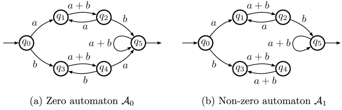
Figure 1: Zero and non-zero automata

Consider two automata ${\cal A}_{0}$ and ${\cal A}_{1}$ illustrated in Figure 1. ${\cal A}_{0}$ is a zero automaton but ${\cal A}_{1}$ is not, though both automata have a sink state $q_{5}$. The only difference between ${\cal A}_{0}$ and ${\cal A}_{1}$ is the transition result of $q_{4}\cdot a$; which equals to $q_{5}$ in ${\cal A}_{0}$, while which equals to $q_{3}$ in ${\cal A}_{1}$. We can easily verify that, ${\cal A}_{0}$ has a unique strongly connected sink component $q_{5}$, while ${\cal A}_{1}$ has two strongly connected sink components $\{q_{3},q_{4}\}$ and $q_{5}$.

Definition 3 can be rephrased as follows.

Lemma 2.

Let ${\cal A}=\langle Q,A,\cdot,q_{0},F\rangle$ be an automaton. Then ${\cal A}$ is zero if and only if ${\cal A}$ has a unique strongly connected sink component and it is trivial, i.e.,  ${\sf{Sink}}({\cal A})=\{\{p\}\}$ for a certain sink state $p$.

Proof.

First we assume ${\cal A}$ is zero with a sink state $p$. Then there exists a synchronising word $w$ and it clearly satisfies $q\cdot w=p$ for each $q$ in $Q$ since $p$ is sink. This shows that there is no strongly connected sink component in $Q\setminus p$.

Now we prove the converse direction, we assume ${\cal A}$ has a unique strongly connected sink component and it is trivial, say $p$. We can verify that for every state $q$ in $Q$, there exists a word $w$ in $A^{*}$, such that $q\cdot w=p$. Indeed, if there does not exist such word $w$ for some $q$, then the set of all reachable states from $q:\{r\in Q\mid\exists w\in A^{*},q\cdot w=r\}$ must contains at least one strongly connected sink component which does not contain $p$. This contradicts with the uniqueness of the closed strongly connected component $p$ in ${\cal A}$. The existence of a synchronising word $w$ is guaranteed, because we can concretely construct it as follows. Let $n$ be the number of states $n=|Q|$ and let $Q=\{q_{0},\cdots,q_{n-1}=p\}$. We define a word sequence $w_{i}$ inductively by $w_{0}=u_{q_{0}}$ and $w_{i}=u_{(q_{i}\cdot v_{i-1})}$ where each $u_{q_{i}}$ is a shortest word satisfies $q_{i}\cdot u_{q_{i}}=p$, and $v_{i-1}$ is the word of the form $w_{0}\cdots w_{i-1}$.

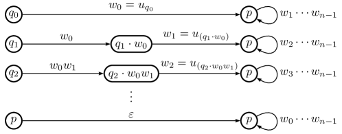
Figure 2: Synchronising word $v_{n-1}=w_{0}\cdots w_{n-1}$ in the proof of Lemma 2

As shown in Figure 2, we can easily verify that the word $v_{n-1}=w_{0}\cdots w_{n-1}$ is a synchronising word satisfies $q\cdot v_{n-1}=p$ for each $q$ in $Q$.

For example, consider the zero automaton ${\cal A}_{0}$ in Figure 1. Then each $u_{q_{i}},w_{q_{i}}$ and $v_{q_{i}}$ are defined as follows.

	$u_{q_{i}}$	$w_{q_{i}}$	$v_{q_{i}}$
$q_{0}$	$aab$	$aab$	$aab$
$q_{1}$	$ab$	$b$	$aabb$
$q_{2}$	$b$	$\varepsilon$	$aabb$
$q_{3}$	$aa$	$\varepsilon$	$aabb$
$q_{4}$	$a$	$\varepsilon$	$aabb$
$q_{5}$	$\varepsilon$	$\varepsilon$	$aabb$

The obtained word $v_{q_{4}}=aabb$ is a synchronising word which satisfies $q_{i}\cdot aabb=q_{5}$ for all $q_{i}$ in ${\cal A}_{0}$. It is clear that the non-zero automaton ${\cal A}_{1}$ in Figure 1 does not have a synchronising word since it has two strongly connected sink components. ∎

4 Closure properties of ${\cal Z\!\!O}$

We first introduce the following lemma.

Lemma 3.

Let $L$ be a language of $A^{*}$ and $w$ be a word in $A^{k}$. Then the asymptotic probability of $L$ exists if and only if the asymptotic probability of the language $wL\;[Lw]$ exists. Moreover, these limits satisfies the equation $\mu(wL)=\mu(Lw)=|A|^{-k}\mu(L)$.

Proof.

Since $wL$ and $Lw$ clearly have the same counting function, we only have to prove the case of $wL$. For every $u,v$ in $A^{k}$ such that $u\neq v$, the language $uL$ and $vL$ are obviously mutually disjoint and these counting functions satisfies

$$\gamma_{n}(uL)=\gamma_{n}(vL)=\begin{cases}0&n<k,\\ \gamma_{n-k}(L)&n\geq k.\end{cases}$$

This shows that $uL$ and $vL$ have the same counting function and thus have the same asymptotic probability if its exists. We can easily verify that

$$\mu(L)=\mu\left(A^{k}L\right)=\sum_{u\in A^{k}}\mu(uL)=|A|^{k}\mu(wL)$$

holds for any $w$ in $A^{k}$. ∎

Now we prove the following proposition, which states the necessary closure properties of the class ${\cal Z\!\!O}$ for Lemma 1.

Proposition 1.

${\cal Z\!\!O}$ is closed under Boolean operations, left and right quotients.

Proposition 1.

We first prove that ${\cal Z\!\!O}$ is closed under Boolean operations, and then prove that ${\cal Z\!\!O}$ is closed under quotients.

${\cal Z\!\!O}$ is closed under Boolean operations.  Let $L,K$ be two languages in ${\cal Z\!\!O}$. It is obvious that ${\cal Z\!\!O}$ is closed under complement since $\mu(\overline{L})=1-\mu(L)\in\{0,1\}$, and we can easily verify that the following equations holds.

• $\mu(L\cup K)=0$ if $\mu(L)=0$ and $\mu(K)=0$;

• $\mu(L\cap K)=0$ if either $\mu(L)=0$ or $\mu(K)=0$;

• $\mu(L\cup K)=1$ if either $\mu(L)=1$ or $\mu(K)=1$;

• $\mu(L\cap K)=1$ if $\mu(L)=1$ and $\mu(K)=1$.

${\cal Z\!\!O}$ is closed under quotients.  We first prove that ${\cal Z\!\!O}$ is closed under left quotients. Let $L$ be a regular language in ${\cal Z\!\!O}$ and we assume that $L$ does not contain $\varepsilon$ without loss of generality. First we assume $\mu(L)=0$. By the definition of left quotients, one can easily verify that

$$L=\bigcup_{a\in A}L\cap aA^{*}=\bigcup_{a\in A}aa^{-1}L$$

holds (since $\varepsilon\notin L$) and all these sets $aa^{-1}L$ $(=L\cap aA^{*})$ are mutually disjoint. It follows that the following equation holds.

$$\mu(L) = \lim_{n\rightarrow\infty}\frac{|L\cap A^{n}|}{|A^{n}|}=\lim_{n\rightarrow\infty}\frac{|\left(\bigcup_{a\in A}aa^{-1}L\right)\cap A^{n}|}{|A^{n}|}=\lim_{n\rightarrow\infty}\frac{|\bigcup_{a\in A}(aa^{-1}L\cap A^{n})|}{|A^{n}|}$$

$$= \lim_{n\rightarrow\infty}\sum_{a\in A}\frac{|aa^{-1}L\cap A^{n}|}{|A^{n}|}=\sum_{a\in A}\mu(aa^{-1}L)=0.$$

That is, the asymptotic probability $\mu(aa^{-1}L)$ equals to zero for each $a$ in $A$, since these summation converges to zero. In addition, $\mu(aa^{-1}L)$ coincides with $\mu(a^{-1}L)$ for any $a$ in $A$, because $\mu(aa^{-1}L)=|A|^{-1}\mu(a^{-1}L)=0$ by Lemma 3 whence $\mu(a^{-1}L)=0$.

Next we assume $\mu(L)=1$. Then $\mu(\overline{L})=0$ and

$$a^{-1}\overline{L}=\{w\in A^{*}\mid aw\in\overline{L}\}=\{w\in A^{*}\mid aw\notin L\}=\overline{a^{-1}L}$$

holds. We therefore obtain:

$$\mu(a^{-1}L)=1-\mu(\overline{a^{-1}L})=1-\mu(a^{-1}\overline{L})=1-0=1.$$

We can prove that ${\cal Z\!\!O}$ is closed under right quotients by the same manner. ∎

5 Equivalence of ${\cal Z\!\!O}$ and ${\cal Z}$

We will use the following lemma, which is a direct consequence of Lemma 1 and Proposition 1.

Lemma 4.

Let $L$ be a regular language in ${\cal Z\!\!O}$, ${\cal A}_{L}=\langle Q,A,\cdot,q_{0},F\rangle$ be its minimal automaton. Then, for any subset $P$ of $Q$ in ${\cal A}_{L}$, its past ${\sf{Past}}(P)$ is also in ${\cal Z\!\!O}$.

Proof.

By Lemma 1, for any subset $P$ of $Q$, its past ${\sf{Past}}(P)$ can be expressed as a finite Boolean combination of languages of the form $Lw^{-1}$. It follows that ${\sf{Past}}(P)$ obeys the zero-one law, since $L$ is in ${\cal Z\!\!O}$ and ${\cal Z\!\!O}$ is closed under Boolean operations and quotients by Proposition 1. ∎

Lemma 4 will be used for proving the direction ${\color[rgb]{1,0,0}\scriptsize\ref{condition:zeroone}⃝}\Rightarrow{\color[rgb]{1,0,0}\scriptsize\ref{condition:za}⃝}$. Now we give a proof.

Proof of Theorem 1.

We show the implication ${\color[rgb]{1,0,0}\scriptsize\ref{condition:za}⃝}\Rightarrow{\color[rgb]{1,0,0}\scriptsize\ref{condition:zero}⃝}\Rightarrow{\color[rgb]{1,0,0}\scriptsize\ref{condition:zeroone}⃝}\Rightarrow{\color[rgb]{1,0,0}\scriptsize\ref{condition:za}⃝}$. The former implication ${\color[rgb]{1,0,0}\scriptsize\ref{condition:za}⃝}\Rightarrow{\color[rgb]{1,0,0}\scriptsize\ref{condition:zero}⃝}\Rightarrow{\color[rgb]{1,0,0}\scriptsize\ref{condition:zeroone}⃝}$ is easy and almost folklore, but we include a proof here to be self-contained.

${\color[rgb]{1,0,0}\scriptsize\ref{condition:za}⃝}\Rightarrow{\color[rgb]{1,0,0}\scriptsize\ref{condition:zero}⃝}$ (${\cal A}_{L}$ is zero $\Rightarrow L$ is with zero).  Let ${\cal A}_{L}=\langle Q,A,\cdot,q_{0},F\rangle$ be the minimal automaton of $L$ and it is zero with a sink state $p$. Let $M$ be the transition monoid of ${\cal A}_{L}$ and $\phi:A^{*}\rightarrow M$ be the syntactic morphism of $L$. Then we can verify that $M$ has a zero element $\bm{0}$ as the transformation $\bm{0}:q\mapsto p$ for all $q$ in $Q$, that is, $\bm{0}$ is the constant map from $Q$ to $p$. The existence of $\bm{0}$ is guaranteed since ${\cal A}_{L}$ is synchronising. Indeed, for any synchronising word $w$, $\phi(w)=\bm{0}$ holds. One can easily verify that $m\bm{0}=\bm{0}m=\bm{0}$ for all $m$ in $M$. This proves that $M$ the syntactic monoid of $L$ has the zero.

${\color[rgb]{1,0,0}\scriptsize\ref{condition:zero}⃝}\Rightarrow{\color[rgb]{1,0,0}\scriptsize\ref{condition:zeroone}⃝}$ ($L$ is with zero $\Rightarrow L$ obeys the zero-one law).  Let $L$ be a regular language in ${\cal Z}$, $M$ be its syntactic monoid with a zero element $\bm{0}$ and $\phi:A^{*}\rightarrow M$ be its syntactic morphism. We choose a word $w_{\bm{0}}$ from the preimage of $\bm{0}$: $w_{\bm{0}}\in\phi^{-1}(\bm{0})$.

Now we prove $\mu(L)=1$ if $w_{\bm{0}}$ in $L$. By the definition of zero, we have

$$\phi(xw_{\bm{0}}y)=\phi(x)\phi(w_{\bm{0}})\phi(y)=\phi(x)\bm{0}\phi(y)=\bm{0}$$

for any words $x,y$ in $A^{*}$. That is, if $w$ contains $w_{\bm{0}}$ as a factor, then $\phi(w)=\phi(w_{\bm{0}})=\bm{0}$ holds and hence $w$ also in $L$. Let $L_{w_{\bm{0}}}=A^{*}w_{\bm{0}}A^{*}$ be the set of all words that contain $w_{\bm{0}}$ as a factor. Then clearly $L_{w_{\bm{0}}}$ is contained in $L$ from which we get $\mu_{n}(L_{w_{\bm{0}}})\leq\mu_{n}(L)$ for all $n$. The probability $\mu_{n}(L_{w_{\bm{0}}})$ is nothing but the probability that a randomly chosen word of length $n$ contains $w_{\bm{0}}$ as a factor. The following well known elementally fact, sometimes called Borges’s theorem (cf. Note I.35 in [11]), ensures that $\mu_{n}(L_{w_{\bm{0}}})$ tends to one if $n$ tends to infinity. This shows $\mu(L)=\mu(L_{w_{\bm{0}}})=1$ and we can prove $\mu(L)=0$ if $w_{\bm{0}}$ not in $L$ by the same manner.

Borges’s theorem. Take any fixed finite set $\Pi$ of words in $A^{*}$. A random word in $A^{*}$ of length $n$ contains all the words of the set $\Pi$ as factors with probability tending to one exponentially fast as $n$ tends to infinity.

${\color[rgb]{1,0,0}\scriptsize\ref{condition:zeroone}⃝}\Rightarrow{\color[rgb]{1,0,0}\scriptsize\ref{condition:za}⃝}$ ($L$ obeys the zero-one law $\Rightarrow{\cal A}_{L}$ is zero).  Let $L$ be a regular language in ${\cal Z\!\!O}$ and ${\cal A}_{L}=\langle Q,A,\cdot,q_{0},F\rangle$ be its minimal automaton, let ${\sf{Sink}}({\cal A}_{L})=\{P_{1},\cdots,P_{k}\}$ for some $k\geq 0$. Our goal is to prove $k=1$ and ${\sf{Sink}}({\cal A}_{L})=\{\{p\}\}$ for a certain sink state $p$. It follows that ${\cal A}_{L}$ is zero by Lemma 2.

For any strongly connected sink component $P_{i}$, there exists a word $w_{i}$ such that $q_{0}\cdot w_{i}$ in $P_{i}$ because ${\cal A}_{L}$ is accessible. Since $P_{i}$ is sink, the language $w_{i}A^{*}$ is contained in ${\sf{Past}}(P_{i})$ from which we get

$$0<\mu(w_{i}A^{*})=|A|^{-|w_{i}|}\mu(A^{*})=|A|^{-|w_{i}|}\leq\mu({\sf{Past}}(P_{i}))$$ (2)

for each $P_{i}$ by Lemma 3. Lemma 4 and Equation (2) implies that the asymptotic probability $\mu({\sf{Past}}(P_{i}))$ surely exists and satisfies

$$\mu({\sf{Past}}(P_{i}))=1$$ (3)

for every strongly connected sink component $P_{i}$.

Now we prove $k=1$. By Equation (3), we can easily verify that

$$\mu\left(\bigcup_{i=1}^{k}{\sf{Past}}(P_{i})\right)=\sum_{i=1}^{k}\mu({\sf{Past}}(P_{i}))=k$$

holds because ${\cal A}_{L}$ is deterministic and thus all ${\sf{Past}}(P_{i})$ are mutually disjoint. This clearly shows $k=1$, that is, there exists a unique strongly connected sink component, say $P$, in ${\cal A}_{L}$: ${\sf{Sink}}({\cal A}_{L})=\{P\}.$

Next we let $P=\{p_{1},\cdots,p_{n}\}$ and prove $n=1$. Since $P$ satisfies $\mu({\sf{Past}}(P))=1$ by Equation (3), there exists exactly one state $p$ in $P$ satisfies $\mu({\sf{Past}}(p))=1$ by Lemma 4. Further, because $P$ is strongly connected, for every state $p_{i}$ in $P$, there exists a word $w_{i}$ such that $p\cdot w_{i}=p_{i}$. It follows that ${\sf{Past}}(p)w_{i}\subseteq{\sf{Past}}(p_{i})$ and thus

$$0<\mu({\sf{Past}}(p)w_{i})=|A|^{-|w_{i}|}\mu({\sf{Past}}(p))=|A|^{-|w_{i}|}\leq\mu({\sf{Past}}(p_{i}))=1$$ (4)

holds for every state $p_{i}$ in $P$ by Lemma 3 and Lemma 4. Equation (3) and (4) implies

$$\mu({\sf{Past}}(P))=\sum_{i=1}^{n}\mu({\sf{Past}}(p_{i}))=\sum_{i=1}^{n}1=n=1,$$

because ${\cal A}_{L}$ is deterministic and thus all ${\sf{Past}}(p_{i})$ are mutually disjoint. We now obtain $n=1$, that is, $P$ is singleton and hence ${\sf{Sink}}({\cal A}_{L})=\{p\}$. That is, ${\cal A}_{L}$ is zero. ∎

Remark 2.

It is interesting that, though we use Borges’s theorem to prove the direction ${\color[rgb]{1,0,0}\scriptsize\ref{condition:zero}⃝}\Rightarrow{\color[rgb]{1,0,0}\scriptsize\ref{condition:zeroone}⃝}$, Theorem 1 is a vast generalisation of Borges’s theorem, since any language of the form $A^{*}KA^{*}$ where $K$ is regular is always recognised by a zero automaton (but the converse is not true). To state Theorem 1 more precisely, by the proof above we can easily verify that, a zero-one language $L$ satisfies $\mu(L)=1\;[\mu(L)=0]$ if and only if its minimal automaton ${\cal A}_{L}$ is zero and the sink state of ${\cal A}_{L}$ is final [non-final].

6 Linear time algorithm for testing the zero-one law

The equivalence of zero-automata and the zero-one law gives us an effective algorithm. For a given $n$-states automaton ${\cal A}$, we can determine whether $L({\cal A})$ obeys the zero-one law by the following steps: (i) Minimise ${\cal A}$ to obtain its minimal automaton ${\cal B}$. (ii) Calculate the family of all strongly connected components $P$ of ${\cal B}$. (iii) Check whether $P$ contains exactly one strongly connected sink component and it is trivial, i.e.,  whether ${\cal B}$ is a zero automaton (Lemma 2). It is well known that Hopcroft’s automaton minimisation algorithm has an $\mathop{\mathrm{O}}(n\log n)$ time complexity and Tarjan’s strongly connected components algorithm has an $\mathop{\mathrm{O}}(n+n|A|)=\mathop{\mathrm{O}}(n)$ complexity where $n|A|$ means the number of edges. Hence we can minimise ${\cal A}$ to obtain ${\cal B}$ in $\mathop{\mathrm{O}}(n\log n)$ on the step (i), and can calculate $P$ in $\mathop{\mathrm{O}}(n)$ on the step (ii). One can easily verify that the step (iii) above can be done in $\mathop{\mathrm{O}}(n)$. To sum up, we have an $\mathop{\mathrm{O}}(n\log n)$ algorithm for testing whether a given regular language obeys the zero-one law, if its is given by an $n$-states deterministic finite automaton. We can obtain, however, more efficient algorithm by avoiding minimisation. In order to do that, there is a need for further investigation of the structure of zero automata.

Quasi-zero automata and more effective algorithm.  Let ${\cal A}=\langle Q,A,\cdot,q_{0},F\rangle$ be an automaton. The Nerode equivalence $\sim$ of ${\cal A}$ is the relation defined on $Q$ by $p\sim q$ if and only if ${\sf{Fut}}(p)={\sf{Fut}}(q)$. One can easily verify that $\sim$ is actually a congruence, in the sense that $F$ is saturated by $\sim$ and $p\sim q$ implies $p\cdot w\sim q\cdot w$ for all $w\in A^{*}$. Hence it follows that there is a well defined new automaton ${\cal A}\!/\!\!\!\sim$, the quotient automaton of ${\cal A}$:

$${\cal A}\!/\!\!\!\sim=\langle Q\!/\!\!\!\sim,A,\cdot,[q_{0}]_{\sim},F\!/\!\!\!\sim\rangle$$

where $[q]_{\sim}$ is the equivalence class modulo $\sim$ of $q$, $S\!/\!\!\!\sim=\{[q]_{\sim}\mid q\in S\}$ is the set of the equivalence classes modulo $\sim$ of a subset $S\subseteq Q$, and where the transition function $\cdot:Q\!/\!\!\!\sim\times A\rightarrow Q\!/\!\!\!\sim$ is defined by $[p]_{\sim}\cdot a=[p\cdot a]_{\sim}$. We define the natural mapping $\phi_{\sim}:Q\rightarrow Q\!/\!\!\!\sim$ by $\phi_{\sim}(q)=[q]_{\sim}$. Condition (M) for minimal automata implies that, for any automaton ${\cal A}$, its quotient automaton ${\cal A}\!/\!\!\!\sim$ is the minimal automaton of $L({\cal A})$. We shall identify the quotient automaton ${\cal A}\!/\!\!\!\sim$ with the minimal automaton of $L({\cal A})$ (cf. [19]).

We now introduce a new class of automata which is a generalisation of the class of zero automata.

Definition 4 (quasi-zero automaton).

An automaton ${\cal A}=\langle Q,A,\cdot,q_{0},F\rangle$ is quasi-zero if either $\bigcup{\sf{Sink}}({\cal A})$ $\subseteq$ $F$ or $\bigcup{\sf{Sink}}({\cal A})\cap F=\emptyset$ holds.

Since every zero automaton ${\cal A}$ satisfies $\bigcup{\sf{Sink}}({\cal A})=\{p\}$ for a certain state $p$ (Lemma 2), every zero automaton is quasi-zero. The following proposition shows that the minimal automaton of any quasi-zero automaton is zero and vice versa (this justifies the term “quasi-zero”).

Proposition 2.

An automaton ${\cal A}=\langle Q,A,\cdot,q_{0},F\rangle$ is quasi-zero if and only if ${\cal A}\!/\!\!\!\sim$ is zero.

Proof.

This proposition shows exactly the equivalence ${\color[rgb]{1,0,0}\scriptsize\ref{condition:za}⃝}\Leftrightarrow{\color[rgb]{1,0,0}\scriptsize\ref{condition:quasi}⃝}$ in Theorem 1.

${\color[rgb]{1,0,0}\scriptsize\ref{condition:za}⃝}\Rightarrow{\color[rgb]{1,0,0}\scriptsize\ref{condition:quasi}⃝}$ (${\cal A}\!/\!\!\!\sim$ is zero $\Rightarrow{\cal A}$ is quasi-zero).  Let $p$ be the unique sink state of ${\cal A}\!/\!\!\!\sim$. To prove this direction, it is enough to consider the case when $p\in F\!/\!\!\!\sim$, i.e.,  ${\sf{Fut}}(p)=A^{*}$. We now show

$$\bigcup{\sf{Sink}}({\cal A})\subseteq F$$ (5)

by contradiction. Let us assume that Inclusion (5) does not hold, that is, we assume there exists a non-final state $q$ in $\bigcup{\sf{Sink}}({\cal A})$. Let $P$ be the strongly connected sink component of ${\cal A}$ that contains $q$. Since $P$ is sink and strongly connected, $\phi_{\sim}(P)$ is sink and strongly connected in ${\cal A}\!/\!\!\!\sim$ too. Moreover, $\phi_{\sim}(P)$ does not contain the sink state $p$, because $q\notin F$ implies that, for any state $q^{\prime}$ in $P$, ${\sf{Fut}}(q^{\prime})\neq A^{*}$ from which we obtain ${\sf{Fut}}([q^{\prime}]_{\sim})\neq{\sf{Fut}}(p)$ and $[q^{\prime}]_{\sim}\neq p$. That is, ${\cal A}\!/\!\!\!\sim$ has at least two strongly connected sink components $\phi_{\sim}(P)$ and $p$. This is contradiction.

${\color[rgb]{1,0,0}\scriptsize\ref{condition:quasi}⃝}\Rightarrow{\color[rgb]{1,0,0}\scriptsize\ref{condition:za}⃝}$ (${\cal A}$ is quasi-zero $\Rightarrow{\cal A}\!/\!\!\!\sim$ is zero).  To prove this direction, it is enough to consider the case when $\bigcup{\sf{Sink}}({\cal A})\subseteq F$. Since ${\cal A}$ is quasi-zero, all states in $\bigcup{\sf{Sink}}({\cal A})$ have the same future $A^{*}$, i.e.,  ${\sf{Fut}}(q)=A^{*}$ for every state $q$ in $\bigcup{\sf{Sink}}({\cal A})$, because $\bigcup{\sf{Sink}}({\cal A})\subseteq F$ implies $q\cdot w\in F$ for every state $q$ in $\bigcup{\sf{Sink}}({\cal A})$ and every word $w$ in $A^{*}$. This implies that $\bigcup{\sf{Sink}}({\cal A})\!/\!\!\!\sim$ consists of a single equivalence class, say $p$. Moreover, this equivalence class $p$ is a sink state in ${\cal A}\!/\!\!\!\sim$ by the definition of sink and Condition (M) of the minimality of ${\cal A}\!/\!\!\!\sim$. We now show that, by contradiction, ${\cal A}\!/\!\!\!\sim$ has only one strongly connected sink component $p$:

$$\bigcup{\sf{Sink}}({\cal A}\!/\!\!\!\sim)=\{p\}$$ (6)

from which we obtain ${\cal A}\!/\!\!\!\sim$ is zero by Lemma 2. Let us assume that Inclusion (6) does not hold, that is, we assume there exists a strongly connected sink component $R=\{r_{1},\cdots,r_{n}\}$ of ${\cal A}\!/\!\!\!\sim$, which does not contain $p$. Recall that each state $r_{i}$ of ${\cal A}\!/\!\!\!\sim$ is an equivalence class, i.e.,  a set of states, of ${\cal A}$. Let $S=\phi_{\sim}^{-1}(R)$ be a set of states of ${\cal A}$. Since $R$ is strongly connected sink component of ${\cal A}\!/\!\!\!\sim$, its preimage $S$ contains at least one strongly connected sink component, say $P$, of ${\cal A}$. For every state $q$ in $P$, ${\sf{Fut}}(q)$ is not equal to $A^{*}={\sf{Fut}}(p)$, because $p\notin\phi_{\sim}(P)\subseteq\phi_{\sim}(S)=R$ implies $[q]_{\sim}\neq p$. This contradicts with the assumption that ${\sf{Fut}}(q)=A^{*}$ for every state $q$ in $\bigcup{\sf{Sink}}({\cal A})$. This completes the proof of Theorem 1. ∎

By using this proposition, we obtain a linear time algorithm by avoiding minimisation as stated in the following theorem.

Theorem 2.

There is an $\mathop{\mathrm{O}}(n)$ algorithm for testing whether a given regular language is zero-one, if its is given by an $n$-states deterministic finite automaton.

Proof.

For a given $n$-states automaton ${\cal A}$, we can determine whether $L({\cal A})$ obeys the zero-one law by the following steps: (i) Calculate the family of all strongly connected components $P$ of ${\cal A}$. (ii) Extract all strongly connected sink components from $P$ to obtain ${\sf{Sink}}({\cal A})$. (iii) Check whether, in $\bigcup{\sf{Sink}}({\cal A})$, either all states are final or all states are non-final, i.e.,  whether ${\cal A}$ is quasi-zero. By Theorem 1, $L({\cal A})$ obeys the zero-one law if and only if ${\cal A}$ is quasi-zero. Hence this algorithm is correct. All steps (i) $\sim$ (iii) can be done in $\mathop{\mathrm{O}}(n)$, this ends the proof. ∎

7 Logical aspects of the zero-one law

There are different manners to define a language: a set of finite words. In the descriptive approach, the words of a language are characterised by a property. The automata approach is a special case of the descriptive approach. Another variant of the descriptive approach consists in defining languages by logical formulae: we regard words as finite structures with a linear order composed of a sequence of positions labeled over finite alphabet. The zero-one law, which is defined in this paper, has been studied extensively in finite model theory (cf. Chapter 12 “Zero-One Laws” of [15]). This notion can be applied to logics over, not only finite words, but also arbitrary finite structures, such as finite graphs: we regard graphs as finite structures with a set of nodes and their edge relation. We say that a logic ${\cal L}$, over fixed finite structures, has the zero-one law if every property $\Phi$ definable in ${\cal L}$ satisfies $\mu(\Phi)\in\{0,1\}$ ($\mu$ is defined analogously). Broadly speaking, every property $\Phi$ is either almost surely true or almost surely false. Fagin’s theorem [10] states that first-order logic $\mathop{\mathrm{FO}}\nolimits$ for finite graphs has the zero-one law. Moreover, an $\mathop{\mathrm{FO}}\nolimits$ sentence $\Phi$ is almost surely true (i.e.,  $\mu(\Phi)=1$) if and only if $\Phi$ is true on a certain infinite graph: the random graph. This characterisation leads to the fact that, for any $\mathop{\mathrm{FO}}\nolimits$ sentence $\Phi$, it is decidable whether $\mu(\Phi)=1$ (cf. Corollary 12.11 in [15]). After the work of Fagin, much ink has been spent on the zero-one law for logics over finite graphs. It is now known that many logics (e.g.,  logic with a fixed point operator [5], finite variable infinitary logic [13] and certain fragments of second-order logic [14]) have the zero-one law.

By contrast, though many logics have the zero-one law, their extensions with ordering (like as logics over finite words), no longer have it. In fact, over both finite graphs and finite words, while first-order logic $\mathop{\mathrm{FO}}\nolimits$ has the zero-one law, its extension with a linear order $\mathop{\mathrm{FO}}\nolimits[<]$ does not.

Example 3.

A simple counterexample is the language $(aA)^{*}$ which can be defined by the $\mathop{\mathrm{FO}}\nolimits[<]$ sentence $\Phi_{aA^{*}}=\exists i\left(\forall j(i<j)\land P_{a}(i)\right).$ The variables $i$ and $j$ of this sentence represent position in a word. The sentence $P_{a}(i)$ is interpreted to mean “the $i$-th letter is $a$”. This language $aA^{*}$ satisfies $\mu_{n}(aA^{*})=1/|A|$ as we stated in Section 1, hence $\Phi_{aA^{*}}$ does not obey the zero-one law in general. It follows that $\mathop{\mathrm{FO}}\nolimits[<]$ for finite words does not have the zero-one law.

We summarise well known logical and algebraic characterisations of classes of languages, including the class of zero-one languages ${\cal Z\!\!O}$, in Figure 3. Details and full proofs of these results can be found in a very nice survey [7] by Diekert et al. In Figure 3, we use standard abridged notation: $\mathop{\mathrm{FO}}\nolimits^{n}[<]$ for first-order logic with $n$ variables; $\Sigma_{n}[<]$ for $\mathop{\mathrm{FO}}\nolimits$ formulae with $n$ blocks of quantifiers and starting with a block of existential quantifiers; $\mathbb{B}\Sigma_{n}[<]$ for the Boolean closure of $\Sigma_{n}[<]$. A monomial over $A$ is a language of the form $A_{0}^{*}a_{1}A_{1}^{*}a_{2}\cdots a_{k}A_{k}^{*}$ where $a_{i}$ in $A$ and $A_{i}\subseteq A$ for each $i$, and is unambiguous if for all $w\in A_{0}^{*}a_{1}A_{1}^{*}a_{2}\cdots a_{k}A_{k}^{*}$ there exists exactly one factorisation $w=w_{0}a_{1}w_{1}a_{w}\cdots a_{k}w_{k}$ with $w_{i}$ in $A_{i}^{*}$ for each $i$. A language $L$ over $A$ is called:

• star-free if it is expressible by union, concatenation and complement, but does not use Kleene star;

• polynomial if it is a finite union of monomials;

• unambiguous polynomial if it is a finite disjoint union of unambiguous monomials;

• piecewise testable if it is a finite Boolean combination of simple polynomials;

• simple polynomial if it is a finite union of languages of the form $A^{*}a_{1}A^{*}a_{2}\cdots a_{k}A^{*}$.

Languages	Monoids	Logic
regular	finite	$\mathop{\mathrm{MSO}}\nolimits[<]$
star-free	aperiodic	$\mathop{\mathrm{FO}}\nolimits[<]$
polynomials		$\Sigma_{2}[<]$
unambiguous polynomials	$\mathbb{DA}$	$\mathop{\mathrm{FO}}\nolimits^{2}[<]$
zero-one	with zero	?
piecewise testable	${\cal J}$-trivial	$\mathbb{B}\Sigma_{1}[<]$
simple polynomial		$\Sigma_{1}[<]$
$\mathbb{B}\{A^{*}\mid A\subseteq\Sigma\}$	commutative and idempotent	$\mathop{\mathrm{FO}}\nolimits^{1}[<]$

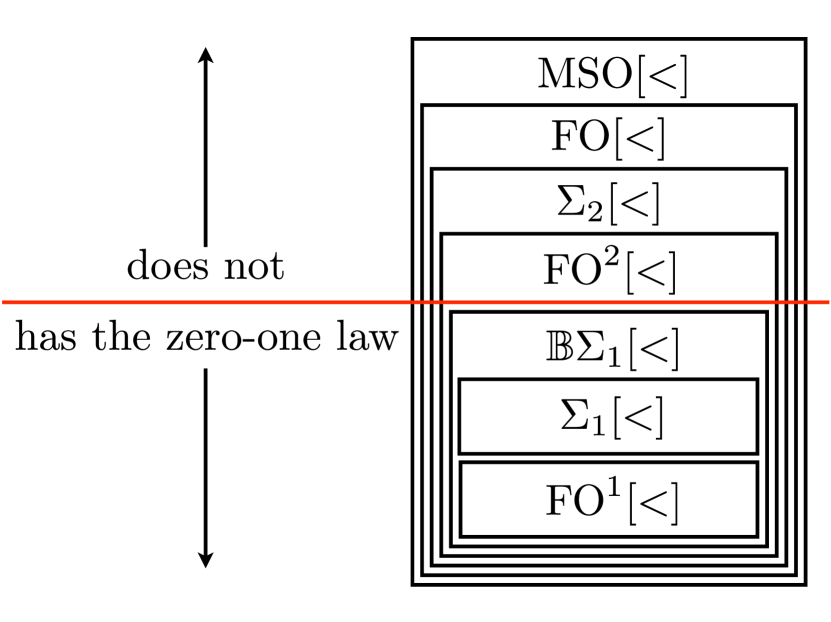
Figure 3: Logical and algebraic characterisations of well known subclasses of regular languages.

The question then arises as to which fragments of $\mathop{\mathrm{FO}}\nolimits[<]$ over finite words have the zero-one law. The algebraic characterisation of the zero-one law partially answers this question. Since every $\cal J$-trivial syntactic monoid has a zero element (cf. [17]), Theorem 1 leads to the following corollary.

Corollary 1.

The Boolean closure of existential first-order logic over finite words has the zero-one law.

One can easily verify that the sentence $\Phi_{aA^{*}}$ in example 3, which only uses two variables $i$ and $j$, is in $\mathop{\mathrm{FO}}\nolimits^{2}[<]$. It follows that $\mathop{\mathrm{FO}}\nolimits^{2}[<]$ does not have the zero-one law, hence Corollary 1 shows us a “separation line” (red line in Figure 3). It must be noted that the class of zero-one languages ${\cal Z\!\!O}$ and unambiguous polynomials are incomparable. To take a simple example, consider two languages $(aa)^{*}$ and $aA^{*}$ over $A=\{a,b\}$. The language $(aa)^{*}$ is zero-one but not unambiguous polynomial since its syntactic monoid is not aperiodic (i.e.,  having no nontrivial subgroup). Conversely, $aA^{*}$ is not zero-one but unambiguous polynomial since it is definable in $\mathop{\mathrm{FO}}\nolimits^{2}[<]$ as we have stated in Example 3. An interesting open problem is whether there exists a logical fragment that exactly captures the zero-one law.

8 Related works

The notion of probability $\mu_{n}$ for regular languages has been studied by Berstel [2] from 1973, and by Salomaa and Soittola [20] from 1978 in the context of the theory of formal power series. They proved that $\mu_{n}(L)$ has finitely many accumulation points and each accumulation point is rational. Another approach, based on Markov chain theory, was presented by Bodirsky et al. [6]. They investigate the algorithmic complexity of computing accumulation points of $L$ and introduced an $\mathop{\mathrm{O}}(n^{3})$ algorithm to compute $\mu(L)$ for any regular language $L$ (and hence whether $L$ is zero-one), if $L$ is given by an $n$-states deterministic finite automaton.

A similar notion, density of a language have also been studied in algebraic coding theory (cf. [3, 4]). A probability distribution $\pi$ on $A^{*}$ is a function $\pi:A^{*}\rightarrow[0,1]$ such that $\pi(\epsilon)=1$ and $\sum_{a\in A}\pi(wa)=\pi(w)$ for all $w$ in $A^{*}$. As a particular case, a Bernoulli distribution is a morphism from $A^{*}$ into $[0,1]$ such that $\sum_{a\in A}\pi(a)=1$. Clearly, a Bernoulli distribution is a probability distribution. We denote by $A^{(n)}=A^{0}\cup A\cup\cdots\cup A^{n-1}$ the set of all words of length less than $n$ over a finite alphabet $A$. The density $\delta(L)$ of $L$ is a limit defined by

$$\delta(L)=\lim_{n\rightarrow\infty}\frac{1}{n}\pi\left(L\cap A^{(n)}\right)$$

where $\pi$ is a probability distribution on $A^{*}$. A monoid $M$ is called well founded if it has a unique minimal ideal, if moreover this ideal is the union of the minimal left ideals of $M$, and also of the minimal right ideals, and if the intersection of a minimal right ideal and of a minimal left ideal is a finite group. An elementary result from analysis shows that if the sequence $\pi(L\cap A^{n})$ has a limit, then $\delta(L)$ also has a limit, and both are equal. The converse, however, does not hold (e.g.,  $\delta((AA)^{*})=1/2$). In their book [4], Berstel et al. proved Theorem 13.4.5 which states that, for any well founded monoid $M$ and morphism $\phi:A^{*}\rightarrow M$, $\delta(\phi^{-1}(m))$ has a limit for every $m$ in $M$. Furthermore, this density is non-zero if and only if $m$ in the minimal ideal $K$ of $M$ from which we obtain $\delta(\phi^{-1}(K))=1$. Since every monoid with zero is well founded, Theorem 13.4.5 implies that, every language with zero is zero-one (i.e.,  ${\color[rgb]{1,0,0}\scriptsize\ref{condition:zero}⃝}\Rightarrow{\color[rgb]{1,0,0}\scriptsize\ref{condition:zeroone}⃝}$, “easy part” of our Theorem 1). Some other related results can be found in the theory of probabilities on algebraic structures initiated by Grenander [12] and Martin-Löf [16].

The point to observe is that the techniques presented in this paper are purely automata theoretic. We did not use any probability theoretic tools, like as measure theory, formal power series, Markov chain, algebraic coding theory, etc. This point deserves explicit emphasise.

Acknowledgement.  I wish to thank the anonymous reviewers for their valuable comments and suggestions to improve the quality of the paper, especially, who informed me the previous works in algebraic coding theory (Theorem 13.4.5 in [4]). Special thanks also go to Prof. Yasuhiko Minamide (Tokyo Institute of Technology) whose meticulous comments for Lemma 1 were an enormous help to me. I am grateful to Prof. Jacques Sakarovitch (Télécom ParisTech) whose comments and suggestions (and his excellent book [19]) were innumerably valuable throughout the course of my study. This work was supported by JSPS KAKENHI Grant Number $26\cdot 11962$.

References

- [1]
- [2] Jean Berstel (1973): Sur la densité asymptotique de langages formels. In: International Colloquium on Automata, Languages and Programming (ICALP, 1972), North-Holland, France, pp. 345–358.
- [3] Jean Berstel & Dominique Perrin (1985): Theory of codes. Pure and applied mathematics, Academic Press, Orlando, San Diego, New York.
- [4] Jean Berstel, Dominique Perrin & Christophe Reutenauer (2009): Codes and Automata (Encyclopedia of Mathematics and Its Applications), 1st edition. Cambridge University Press, New York, NY, USA.
- [5] Andreas Blass, Yuri Gurevich & Dexter Kozen (1985): A Zero-One Law for Logic with a Fixed-Point Operator. Information and Control 67(1-3), pp. 70–90, 10.1016/S0019-9958(85)80027-9.
- [6] Manuel Bodirsky, Tobias Gärtner, Timo von Oertzen & Jan Schwinghammer (2004): Efficiently Computing the Density of Regular Languages. In Martín Farach-Colton, editor: LATIN 2004: Theoretical Informatics, Lecture Notes in Computer Science 2976, Springer Berlin Heidelberg, pp. 262–270, 10.1007/978-3-540-24698-5_30.
- [7] Volker Diekert, Paul Gastin & Manfred Kufleitner (2008): A Survey on Small Fragments of First-Order Logic over Finite Words. International Journal of Foundations of Computer Science 19(3), pp. 513–548, 10.1142/S0129054108005802.
- [8] Samuel Eilenberg & Bret Tilson (1976): Automata, languages and machines. Volume B. Pure and applied mathematics, Academic Press, New-York, San Franciso, London.
- [9] Zoltán Ésik & Masami Ito (2003): Temporal Logic with Cyclic Counting and the Degree of Aperiodicity of Finite Automata. Acta Cybernetica 16(1), pp. 1–28. Available at http://www.inf.u-szeged.hu/actacybernetica/edb/vol16n1/Esik_2%003_ActaCybernetica.xml.
- [10] Ronald Fagin (1976): Probabilities on Finite Models. J. Symb. Log. 41(1), pp. 50–58, 10.1017/S0022481200051756.
- [11] Philippe Flajolet & Robert Sedgewick (2009): Analytic Combinatorics, 1 edition. Cambridge University Press, New York, NY, USA, 10.1017/CBO9780511801655.
- [12] Ulf Grenander (1963): Probabilities on algebraic structures. Wiley, New York.
- [13] Phokion G. Kolaitis & Moshe Y. Vardi (1992): Infinitary logics and 0–1 laws. Information and Computation 98(2), pp. 258 – 294, 10.1016/0890-5401(92)90021-7. Available at http://www.sciencedirect.com/science/article/pii/089054019290%0217.
- [14] Phokion G. Kolaitis & Moshe Y. Vardi (2000): 0-1 Laws for Fragments of Existential Second-Order Logic: A Survey. In Mogens Nielsen & Branislav Rovan, editors: MFCS, Lecture Notes in Computer Science 1893, Springer, pp. 84–98, 10.1007/3-540-44612-5_6. Available at http://dblp.uni-trier.de/db/conf/mfcs/mfcs2000.html#KolaitisV%00.
- [15] Leonid Libkin (2004): Elements of Finite Model Theory. SpringerVerlag, 10.1007/978-3-662-07003-1.
- [16] Per Martin-Löf (1965): Probability theory on discrete semigroups. Zeitschrift für Wahrscheinlichkeitstheorie und Verwandte Gebiete 4(1), pp. 78–102, 10.1007/BF00535486.
- [17] Jean-Éric Pin: Mathematical foundations of automata theory. Available at http://www.liafa.jussieu.fr/~jep/PDF/MPRI/MPRI.pdf.
- [18] Igor Rystsov (1997): Reset words for commutative and solvable automata. Theoretical Computer Science 172(1–2), pp. 273 – 279, 10.1016/S0304-3975(96)00136-3.
- [19] Jacques Sakarovitch (2009): Elements of Automata Theory. Cambridge University Press, New York, NY, USA, 10.1017/CBO9781139195218.
- [20] Arto Salomaa & M. Soittola (1978): Automata Theoretic Aspects of Formal Power Series. Springer-Verlag New York, Inc., Secaucus, NJ, USA, 10.1007/978-1-4612-6264-0.