The Team Keck Redshift Survey 2: MOSFIRE Spectroscopy of the GOODS-North Field

Abstract

We present the Team Keck Redshift Survey 2 (TKRS2), a near-infrared spectral observing program targeting selected galaxies within the CANDELS subsection of the GOODS-North Field. The TKRS2 program exploits the unique capabilities of MOSFIRE, an infrared multi-object spectrometer which entered service on the Keck I telescope in 2012 and contributes substantially to the study of galaxy spectral features at redshifts inaccessible to optical spectrographs. The TKRS2 project targets 97 galaxies drawn from samples that include $z\approx 2$ emission-line galaxies with features observable in the $JHK$ bands as well as lower-redshift targets with features in the $Y$ band. We present a detailed measurement of MOSFIRE’s sensitivity as a function of wavelength, including the effects of telluric features across the $YJHK$ filters. The largest utility of our survey is in providing rest-frame-optical emission lines for $z>1$ galaxies, and we demonstrate that the ratios of strong, optical emission lines of $z\approx 2$ galaxies suggest the presence of either higher N/O abundances than are found in $z\approx 0$ galaxies or low-metallicity gas ionized by an active galactic nucleus. We have released all TKRS2 data products into the public domain to allow researchers access to representative raw and reduced MOSFIRE spectra.

1 Introduction

The peak of the cosmic star-formation rate (SFR) occurs at $z\approx 2$ (e.g., Madau & Dickinson, 2014), but the star-formation processes occurring in galaxies observed at that epoch differ significantly from those occurring in galaxies seen today. In contrast to galaxies such as the Milky Way which form stars continuously in giant molecular clouds, $z>1$ galaxies may be dominated by discrete and recurrent starbursts (e.g., Papovich et al., 2005). The dynamics of most $z>1$ galaxies are also frequently disordered (Kassin et al., 2012), exhibiting clumps of high-pressure gas or young stars (e.g., Cowie, Hu & Songaila, 1995; Elmegreen, Elmegreen & Hirst, 2004; Guo et al., 2012, 2015), unlike the smoother, rotation-dominated disks of massive, star-forming galaxies observed at the present epoch. Reconciling the disparate properties of present-day galaxies with those observed at $z>1$ remains an active and crucial research topic for tracking galaxy evolution.

Rest-frame optical spectroscopy offers a powerful means to probe the physical conditions of galaxies by potentially revealing the evolutionary pathways at play for $z\approx 2$ galaxies. In addition to measuring redshifts needed for deriving basic galaxy properties such as light and stellar mass, rest-frame-optical spectra provide emission lines that probe the SFR (e.g., Kennicutt, 1998), gas-phase metallicity (e.g., Kewley et al., 2001), and nuclear activity of galaxies (e.g., Baldwin, Phillips & Terlevich, 1981; Veilleux & Osterbrock, 1987; Kewley et al., 2006). At $z>1$, rest-frame-optical features are redshifted into the near infrared, a wavelength regime in which observations were once limited to single-slit spectrographs; thus, completing near-IR redshift surveys has historically been prohibitively time-intensive. The advent of multi-object, near-IR spectrographs on 8–10 m-class telescopes has recently enabled several new surveys of rest-frame-optical emission lines in $z>1$ galaxies (e.g., Yoshikawa et al., 2010; Brammer et al., 2012; Kashino et al., 2013; Trump et al., 2013; Steidel et al., 2014; Kriek et al., 2015; Wisnioski et al., 2015).

In this work, we present the Team Keck Redshift Survey 2 (TKRS2), a spectroscopic survey of 97 distant galaxies exploiting the unique capabilities of the MOSFIRE spectrometer on the Keck I telescope. Section 2 describes the key characteristics enabling MOSFIRE to complete infrared spectroscopic surveys of the type previously limited to optical spectrometers. In §3 we describe the mask design and target selection, and §4 details the spectroscopic observations, data reduction, and method for determining redshifts. The redshift catalog appears in §5. We present some basic analyses of the spectroscopic data in §6, including a characterization of the MOSFIRE sensitivity across the $YJHK$ filters, comparison to previous redshifts, and a discussion of the galaxies’ rest-frame optical emission-line ratios.

2 The MOSFIRE Spectrometer

Our survey relies on the unique capabilities of the W. M. Keck Observatory’s newest instrument, the Multi-Object Spectrometer For Infra-Red Exploration (MOSFIRE, McLean et al., 2012). MOSFIRE combines flexible multi-slit spectroscopy capability with high throughput, making it the ideal near-infrared instrument for studying the faintest and most distant galaxies. MOSFIRE features a $2048\times 2048$ pixel HAWAII-2RG HgCdTe detector array from Teledyne Imaging Sensors that couples high quantum efficiency with low noise and low dark current. The operating range of 0.97–2.41 $\micron$ covers the $YJHK$ infrared passbands, with wavelength coverage of 0.97–1.12 µm in $Y$, 1.15–1.35 µm in $J$, 1.47–1.80 µm in $H$, and 1.95–2.40 µm in $K$. Observers can acquire spectra in any one of these passbands by setting the diffraction grating and order-sorting filters appropriately, although simultaneous observations in multiple passbands (cf. VLT’s XSHOOTER; Vernet et al., 2011) are not possible. The resolving power for the default slit width of $0\farcs 7$ is $R$ = 3,380 in $Y$, 3,310 in $J$, 3,660 in $H$, and 3,620 in $K$, corresponding to FWHM spectral resolutions of 3.1 Å in $Y$, 3.7 Å in $J$, 4.4 Å in $H$, and 6.0 Å in $K$.

The feature which most distinguishes MOSFIRE from other slit spectrographs — optical as well as infrared — is the configurable slit mechanism residing within its cryogenic dewar. Previous IR multi-slit spectrometers have relied on custom-milled slitmasks that required thermal cycling of the dewar for installation and removal. In contrast, the MOSFIRE Configurable Slit Unit (CSU) is a fully-robotic mechanism which is remotely controlled and allows the instrument to remain at cryogenic operating temperature throughout each observing run, yielding observations of greater stability. The CSU mechanism puts 92 pairs of matching bars in the re-imaged telescope focal plane, forming up to 46 separate slits of length $7\farcs 0$ that can be positioned independently within the $6\farcm 1\times 6\farcm 1$ MOSFIRE field of view, or can be combined to form longer slits. The MOSFIRE mask design software includes a target prioritization scheme, and the sky density of our faint ($H\lesssim 24$) galaxy targets normally resulted in 25–30 targets being assigned to slits on each mask. The width of each slit can be precisely and independently adjusted based on the needs of the observing program; however, we employed a consistent slit width of $0\farcs 7$ in the present survey to balance the competing desires for improved resolution (dictating narrower slits) and throughput (requiring wider slits). MOSFIRE observers can easily adjust slit widths during the course of a night to account for variations in seeing conditions, although a slit width of $0\farcs 7$ is generally a good match to the customary excellent ($\sim 0\farcs 5$) Maunakea seeing in the near-IR.

The MOSFIRE CSU also enables a novel mask alignment technique. Many telescopes — Keck I and II included — cannot be positioned to better than the standard slit width based on telescope encoders or guider-based alignment techniques, nor can most instruments be set to the precisely correct rotator angle based on positional feedback alone. The common strategy for aligning a multi-slit layout with the corresponding (faint) sky targets is to include two or more “alignment boxes” on a slitmask; each box is placed at the expected location of a star with accurately known astrometric position (e.g., Kassis et al., 2012). When observers select alignment stars to be much brighter than the faint science targets, short images acquired with the mask in place show the locations of the stars relative to the edges of each alignment box, thereby indicating the rotation and decentering of the mask relative to the alignment stars (and, thus, to the science targets). Ideally, small adjustments of the telescope pointing and instrument rotator angle by appropriate amounts lead to optimal alignment within a couple of iterations. Dedicating space on the mask for alignment boxes does, however, sacrifice area that could be devoted to science slits.

In contrast to this customary method, the procedure of aligning MOSFIRE’s slits with the corresponding sky targets exploits the CSU’s ability to reposition the slits in real time. When setting up on a given field, the observer commands the CSU to recast several (generally 3–4) of the bar pairs to form “alignment boxes” that are actually just extra-wide slits (normally $4\arcsec\times 7\arcsec$). After obtaining alignment between these alignment boxes and their corresponding stars, the observer commands the bar pairs to return to their science configuration to form slits that will collect spectra of science targets. As a result, the full complement of MOSFIRE slits can be devoted to science observations. Given the benefits that the MOSFIRE CSU offers over traditional slitmask spectroscopy, we anticipate that future optical and IR spectrometers will exploit this technology.

3 Target Selection & Mask Design

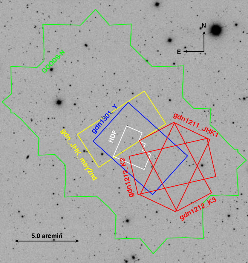
Figure 1: TKRS2 survey fields shown against an image of the GOODS-North field obtained from the Sloan Digital Sky Survey (SDSS, York et al., 2000). The small white polygon indicates the approximate boundary of the HDF-North imaging survey region, and the green polygon denotes the GOODS-North ACS imaging survey region. The red, yellow, and blue rectangles indicate the fields of the TKRS2 survey. The image is oriented with north up and east to the left, with angular scale as indicated by the bar at lower left.

We designed the TKRS2 project to test the capabilities of MOSFIRE on diverse categories of extragalactic sources. Our survey targets the south-central region of the GOODS-North survey field (see Fig. 1; Giavalisco et al., 2004), an area in which the CANDELS program (Grogin et al., 2011) has compiled a superb set of complementary data from the Hubble Space Telescope (HST) and other observatories operating in regimes from radio to X ray. We obtained reset-frame-optical spectra for a sample of galaxies in the redshift range $0.5<z<2.5$, gathering observations in all four of MOSFIRE’s $YJHK$ filters with varying exposure times. Nearly all (90 of 97) of the sources are galaxies without previous high-resolution near-IR spectroscopy. We describe each target category below.

• emline: 83 galaxies expected to show emission lines ([O II] $\lambda\lambda 3726,3729$ Å, H$\beta$ $\lambda 4861$ Å, [O III] $\lambda\lambda 4959,5007$ Å, H$\alpha$ $\lambda 6563$ Å, [N II] $\lambda\lambda 6548,6583$ Å, or [S II] $\lambda\lambda 6717,6731$ Å) at the appropriate redshifts to be observable in the $Y$, $J$, $H$, or $K$ bands. Two thirds of these sources have prior spectroscopic redshifts from optical surveys (Wirth et al., 2004; Reddy et al., 2006; Barger et al., 2008; Ferreras et al., 2009; Cooper et al., 2011) or estimated redshifts derived from low-resolution, near-IR HST/WFC3 G141 grism observations (B. J. Weiner, P.I.). Observing these targets with MOSFIRE adds new, rest-frame-optical emission lines useful for characterizing the physical gas conditions of these galaxies. The remainder have photometric redshifts based on the CANDELS multi-wavelength catalog (Barro et al., in preparation); we included such objects on the masks at substantially lower priority. We also selected extended and clumpy galaxies to test the ability of the routinely excellent Maunakea seeing coupled with with MOSFIRE’s high spectral resolution to generate resolved kinematic measurements.

• moircs: seven galaxies, each of which had previous Subaru+MOIRCS $H$ or $K$ observations (Yoshikawa et al., 2010). We included these targets primarily to test the performance and efficiency of MOSFIRE compared to MOIRCS in $H$ and $K$ (see Fig. 9), but we also observed in other passbands to access additional emission lines. The “moircs” galaxies are similar to the bright galaxies in the “emline” category.

• quiescent: seven galaxies having spectral energy distributions (SEDs) indicative of quiescent stellar populations (i.e., with low specific SFR) and intended as targets for $Y$-band spectroscopy. We selected these galaxies based on their SFR and $U-V$ vs. $V-J$ rest-frame colors ($UVJ$ criterion; e.g., Williams et al. 2009). We also required the quiescent galaxy targets to have photometric redshifts of $0.9<z<1.3$ in order to test the capability of MOSFIRE for measuring absorption lines (e.g., Ca II H$+$K $\lambda$4000 Å, H$\delta$, H$\beta$ and Mg II B $\lambda$5178 Å) in the $Y$ band. In general, the 1 h depth of the observations resulted in only tentative absorption line detections, requiring deeper observations to confirm. Interestingly, the spectra of 3 quiescent galaxies include weak emission lines, consistent with (in each case) a weak MIPS 24 $\mu$m flux, a weak X-ray detection, and a nearby star-forming neighbor.

We designed spectroscopic masks for observations in the $Y$, $J$, $H$, and $K$ MOSFIRE observing bands. On the $Y$ mask, we assigned highest priority to the low-density “quiescent” galaxies. We then filled the remaining slits on the mask with “emline” galaxies having spectroscopic redshifts (from TKRS and Barger et al. (2008)) in the range $0.5<z<0.7$, such that H$\alpha$, [N II], and/or [S II] are visible in the $Y$ band. The $Y$ mask included 32 targets, a high target density given the maximum of 46 slits available on MOSFIRE.

We designed two masks to observe in each of $J$, $H$, and $K$. We designed an additional two masks for $K$ observations only, with different position angles (by 40–$80\arcdeg$) such that at least one mask would place a slit within $40\arcdeg$ of a galaxy’s kinematic axis. Kinematic analysis of these multi-orient slit observations will be presented in future work (Simons et al., in preparation). In selecting specific targets, we gave highest priority to the “moircs” galaxies, and assigned “emline” sources in the redshift range $2.1<z<2.6$ to the remaining slits. At these redshifts, [O II] lines lie in $J$, H$\beta$ and [O III] in $H$, and H$\alpha$, [N II], and [S II] in $K$. About two thirds of the targeted emission-line galaxies have redshifts derived from low-resolution HST/WFC3 G141 grism observations (B. J. Weiner, P.I.). We selected these sources over those having only photometric redshifts, and gave slightly higher priority to galaxies with visibly extended and clumpy morphologies (based on imaging from the CANDELS project; Grogin et al., 2011; Koekemoer et al., 2011) in order to test the capabilities of MOSFIRE for studying internal galaxy kinematics.

The next sections discuss the observations and data reduction of the survey. Overall, the survey achieved high redshift completeness ($>80\%$) for emission-line galaxies (“emline” and “moircs” categories) but had marginal success on quiescent targets.

4 Spectroscopy

4.1 Observations

Former WMKO Director Taft Armandroff generously contributed several nights of his Director’s discretionary observing time allocation toward this campaign. Its principal aims were to complement our previous optical survey of the GOODS-North field (Wirth et al., 2004), demonstrate the capabilities of the new MOSFIRE instrument on the Keck I telescope, and establish a public resource by releasing all data products from the survey to the astronomical community. We employed MOSFIRE to acquire spectra in the GOODS-North field over a series of partial nights spanning the period from November 2012 to May 2013. Table 1 summarizes the observations.

To facilitate accurate subtraction of sky and instrumental background emission, spectroscopic observing sequences consisted of a series of dithered exposures alternating between two positions symmetrically offset from the initial pointing. We employed individual exposure times totaling 180 s on-sky integration time in the $Y$ and $K$ bands; given the relatively greater temporal instability of telluric emission in the $J$ and $H$ bands, we reduced integration times at these wavelengths to 120 s. To confirm that the slits remained well aligned with the faint science targets throughout exposure sequences generally lasting an hour or more, mask designs generally included one slit intended to acquire the spectrum of a star which was significantly brighter than the target galaxies. The relatively bright (high S/N) stellar spectrum has multiple applications: monitoring the transparency of the sky; indicating the accuracy of the frame-to-frame telescope dithers along the slit; tracking any pointing drifts during the exposures along the slit direction; recording the variable atmospheric absorptions after normalizing the continuum to a best-fit stellar spectral type; and tracking the pointing offsets perpendicular to the slit by determining the offsets between the telluric absorption wavelengths to that of the telluric emission lines that fill the slit. The data reduction adopted for this work as described in §4.2 only exploits the information on the dithers along the slit. More advanced reductions (see, e.g., Kriek et al., 2015) are possible but beyond the scope of this release.

In keeping with common MOSFIRE practices, we acquired a standard series of dome flatfield exposures in each passband in order to characterize the instrumental response. In the $K$ band, we also acquired dome exposures with no dome-flat illumination, thus isolating the thermal component of the dome emission. Given the prevalence of strong telluric emission in the $Y$, $J$, and $H$ bands which serve to calibrate the wavelength scale, we acquired no arc lamp exposures in these passbands. We also obtained arc lamp exposures for wavelength determination in the $K$ band due to the relatively weaker telluric emission features at longer wavelengths.

4.2 Data Reduction

We processed all images using the MosfireDRP data reduction pipeline written by the MOSFIRE instrument development team and generously shared with the observing community. The pipeline is specifically designed to accommodate dithered spectra. The reduction procedure virtually eliminates contamination from telluric emission lines by independently combining observations from each of the two pointings, scaling the combined images by the exposure time, shifting the images by the dither amount, and computing the difference. By default, the pipeline derives the wavelength solution for the two-dimensional (2-D) spectra using only the telluric emission lines. We also experimented with using arc lamp lines to derive wavelength solutions in the $K$ band, which has comparatively weaker telluric emission features than the shorter-wavelength bands. Using the arc lamp data for calibration resulted in identical wavelength solutions, and so we retained the standard wavelength calibration using telluric lines in our final reduced spectra.

The end result of the MosfireDRP pipeline is a sky-subtracted, wavelength-calibrated, rectified 2-D spectrum for each slit. To create one-dimensional (1-D) spectra, we used custom software to fit a Gaussian function to the wavelength-collapsed image profile, constraining the peak to lie within $\pm 5$ pixels of the expected object position. We extracted the 1-D spectra from a inverse-variance-weighted co-add within a boxcar window centered on the best-fit peak and with a width $1.5\times$ the Gaussian full-width-half-maximum (FWHM). Within a single MOSFIRE filter, the 2-D spectral trace is tilted by $\lesssim 1$ pixel, and so the flat trace used by our extraction method results in reasonable 1-D spectra.

4.3 Redshift Determination

To estimate the redshifts of the targets, at least two team members independently used the Specpro software package (Masters & Capak, 2011) to inspect each of the MOSFIRE spectra. This software allows the user to fit various template spectra to the observed spectra interactively. We made use of the prior redshift information for each target from optical spectroscopy (Wirth et al., 2004; Reddy et al., 2006; Barger et al., 2008; Ferreras et al., 2009; Cooper et al., 2011) and IR grism spectroscopy (B. J. Weiner, P.I.), along with the estimated “photo-z” redshifts derived from multiband photometry (Barro et al., in preparation).

Reviewers recorded both the derived MOSFIRE redshift, $z_{M}$, and a redshift quality parameter, $Q_{M}$, which denotes the reviewer’s confidence in the redshift estimate. Values of $Q_{M}$ are as follows:

• 0: no reported redshift due to lack of identifiable features;

• 1: speculative redshift based on a single line which is faint and/or blended with a sky feature;

• 2: ambiguous redshift based on a single line that does not match the photometric redshift;

• 2.5: ambiguous redshift based on a single line that matches (within $\Delta z/z<0.15$) the prior photometric redshift;

• 3: secure ($P>95\%$) redshift, typically including one strong emission feature and one or more additional weak features; and,

• 4: highly secure ($P>99\%$) redshift, generally exhibiting multiple strong emission features.

After reviewing all targets, we collated the results, re-inspected each target for which the derived redshift or quality code differed, and reached consensus on a final redshift and quality code. Table 2 indicates the number of galaxies receiving each classification.

5 Redshift Catalog

We present the results of our survey in Table 3 and on the website devoted to the survey. In addition to the target identification and position, the table lists the class to which the target belongs and the apparent AB magnitude of the target in HST imaging. Observational data from the TKRS2 survey includes the list of MOSFIRE passbands in which we observed the target, the total MOSFIRE exposure time devoted to the target, and which spectral features we identified in the MOSFIRE spectra. Finally, several sources of redshift information appear in the table, including the presumed redshift of the target from previous spectroscopic surveys (when available) and the source of that prior redshift, the estimated redshift of the source derived via multiband photometry from the CANDELS survey, the redshift derived from the present survey (accounting for prior information), and the redshift quality code, $Q_{M}$, as described in §4.3.

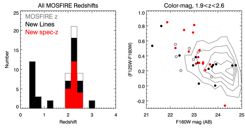
Figure 7: At left, a histogram showing the distribution of spectroscopic redshifts from our program. The open histogram shows the full set of high-confidence ($Q_{M}\geq 3$) MOSFIRE redshifts. The filled red histogram shows the set of targets without previous redshifts from optical spectroscopy, and the black filled histogram shows galaxies with new rest-frame optical emission-line measurements. At right, the $J-H$ vs. $H$ color-magnitude diagram for galaxies with MOSFIRE redshifts of $1.9<z<2.6$ (circles) and the larger galaxy population with photometric redshifts in the same range (gray contours and points). Gray circles indicate galaxies with previous MOIRCS redshifts, filled red circles denote targets with new spectroscopic redshifts, and filled black circles designate galaxies with new rest-frame optical lines. Our sources are more likely to have $H<24$ than the larger population, but otherwise span the same range of $J-H$ colors (roughly corresponding to rest-frame $U-B$ in this redshift range).

The distribution of high-quality ($Q_{M}\geq 3$) redshifts from our survey is shown in Fig. 7 (left panel). For nearly all of the galaxies with high-quality redshifts, our program provides the first spectra with rest-frame optical emission lines. The only sources with previous near-IR spectroscopy (of moderate resolution) are the seven “moircs” targets, which we included for comparison of Keck+MOSFIRE with Subaru+MOIRCS; see §6.2. The right panel of Fig. 7 presents a color-magnitude diagram comparing our $1.9<z<2.6$ galaxies to the larger population of galaxies with photometric redshifts in the same range. Galaxies with high-quality ($Q_{M}\geq 3$) MOSFIRE redshifts tend to have $H<24$, but are otherwise representative of the color distribution for the larger population.

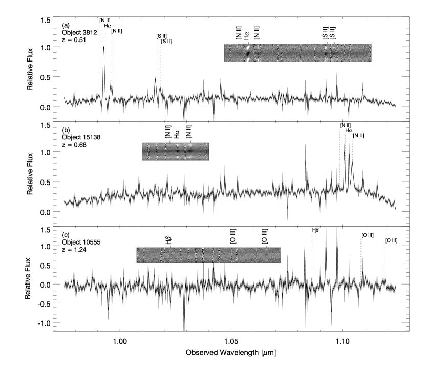
Figure 11: Representative MOSFIRE $Y$-band (near-IR) spectra. Shaded region indicates $\pm 1\sigma$ uncertainty in the spectrum; labels indicate expected locations of notable emission-line features. We applied five-pixel boxcar smoothing to 1-D spectra. Insets show a portion of the corresponding 2-D spectrum to illustrate key emission features, with expected locations of features marked. (a) Object 3812 is a typical $z\approx 0.5$ galaxy showing H$\alpha$, [N II], and [S II] emission, all apparent in the 2-D inset. (b) Object 15138, an X-ray source, lies at somewhat higher redshift; inset shows H$\alpha$ and [N II]. (c) Object 10555 at $z=1.24$ has faintly visible [O III] $\lambda$5007 Å and H$\beta$ features, apparent in the inset; a terrestrial emission line obscures the [O III] $\lambda$4959 Å feature. Confirming optical spectra provide confidence in the redshift despite the relatively low S/N.

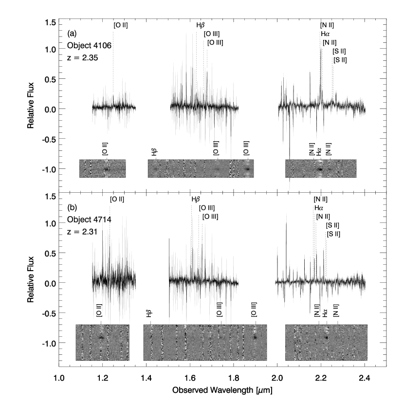
Figure 12: Spectra representative of observations acquired in MOSFIRE’s $JHK$ passbands. As in Fig. 11, we applied five-pixel boxcar smoothing to supress random noise in the 1-D spectra. (a) The spectrum of object 4106 (an X-ray source) shows [O II] visible in the MOSFIRE $J$ band, H$\beta$ and [O III] in $H$, as well as H$\alpha$, [N II], and [S II] emission in $K$. (b) Object 4714 is similar but with relatively fainter features.

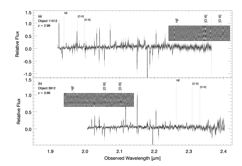
Figure 13: Spectra representative of observations of high-redshift targets observed in MOSFIRE’s $K$ passband. As in Fig. 11, we applied five-pixel boxcar smoothing to supress random noise in the 1-D spectra. (a) Object 11012 is a redshift $z=2.99$ X-ray source, though it has only weak emission lines. (b) The $z=3.66$ redshift of object 3912 is confirmed on the basis of the [O III] $\lambda$5007 Å emission line faintly visible in the 2-D inset.

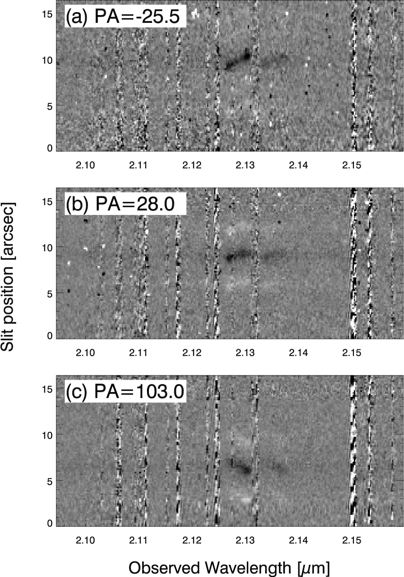
Figure 15: $K$-band MOSFIRE spectra we obtained at each of the three slit position angles indicated in Fig. 14. Visible in the spectra are the emission lines H$\alpha$ $\lambda$6563 Å (redshifted to $2.130~{}\micron$) and [N II] $\lambda$6583 Å (observed at $2.136~{}\micron$). Note that the velocity profile of the lines changes with position angle, allowing detailed investigation of the rotational properties of the target.

Representative spectra from the survey appear in Fig. 11, depicting the $Y$ band, Fig. 12, displaying $JHK$, and Fig. 13, presenting $K$-only spectra. Additionally, Figs. 14 and 15 illustrate the benefit of observing the same target at multiple position angles in order to gain information about the rotational properties of distant galaxies.

6 Analysis

6.1 MOSFIRE Sensitivity

We characterize the sensitivity of MOSFIRE as the flux limit to detect an emission line at the 3$\sigma$ level in 1 h of on-target integration. The flux limit is not constant with wavelength, but instead depends strongly on the presence of telluric emission features. For each filter, we empirically measure the pixel-by-pixel noise as the normalized median absolute deviation (NMAD) from the set of all continuum-subtracted spectra taken in each filter. The noise spectrum is converted from detector units to flux density using the detector response function (available on the Keck MOSFIRE throughput webpage) and a conversion between $e^{-}~{}\mathrm{s}^{-1}$ and flux density measured from twelve $z\approx 1.5$ galaxies with the same emission lines measured by both MOSFIRE and the HST/WFC3 G141 grism. By flux-calibrating with the WFC3 slitless grism we implicitly include a slit loss correction (for galaxies of similar angular size as the twelve $z\approx 1.5$ galaxies). The slit loss correction is typically a factor of 1.5–1.7 (Kriek et al., 2015). We then convolve the noise with a Gaussian, assuming a redshifted H$\alpha$ emission line with rest-frame width $\sigma=85~{}\mathrm{km~{}s}^{-1}$ ($\mathrm{FWHM}=200~{}\mathrm{km~{}s}^{-1}$). This process results in the noise of the fiducial Gaussian emission line centered at each pixel.

Figure 10 presents the $3\sigma$ emission line flux limit in a 1 h exposure, as a function of line-center wavelength across the $YJHK$ filters. The 1 h $3\sigma$ flux limit of MOSFIRE is $\sim 1\times 10^{-17}\mathrm{~{}erg~{}s}^{-1}\mathrm{~{}cm}^{-2}$ in regions with no sky lines in the $YJH$ filters, and up to ten times shallower in regions with strong telluric features. In the $K$ filter, the sensitivity decreases from $\sim 4\times 10^{-17}\mathrm{~{}erg~{}s}^{-1}\mathrm{~{}cm}^{-2}$ in the blue end to $\sim$$6\times 10^{-17}\mathrm{~{}erg~{}s}^{-1}\mathrm{~{}cm}^{-2}$ in the red end of the filter. These Keck/MOSFIRE emission-line sensitivities are very similar to those reported by the MOSDEF survey (Kriek et al., 2015).

6.2 Comparison with Previous Redshifts

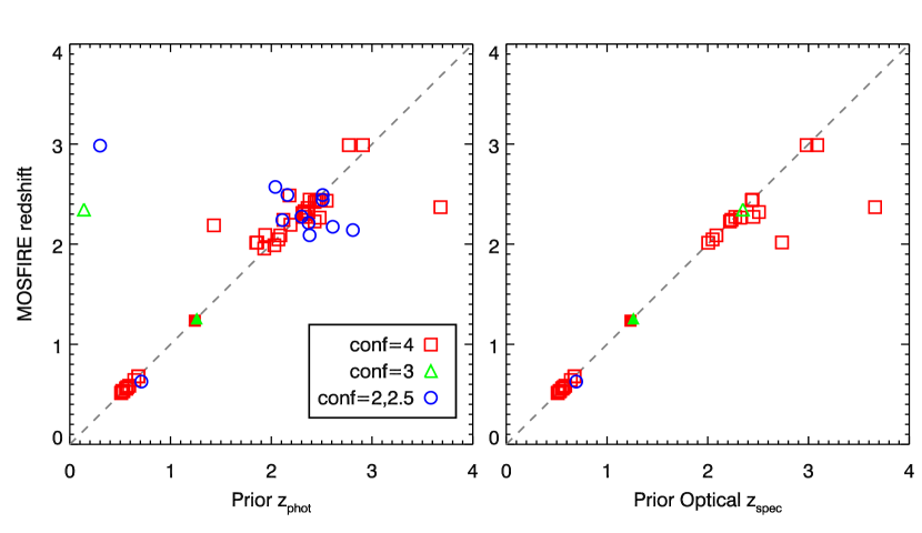
Figure 8: A comparison of our MOSFIRE redshifts with prior photometric redshifts (left panel) and spectroscopic redshifts from prior optical surveys (right panel). Most galaxies have excellent agreement between the MOSFIRE and prior redshifts. At $2<z<3$, prior photometric redshifts and spectroscopic redshifts (based on rest-frame UV spectra) are somewhat more uncertain, and the rest-frame optical emission lines identified by MOSFIRE result in significantly improved redshifts.

We compare the MOSFIRE redshifts with the prior photometric redshifts of our objects in the left panel of Fig. 8. Photometric redshifts come from the CANDELS multiwavelength catalog in GOODS-N (Barro et al., in preparation), using UV-to-NIR spectral energy distributions (SEDs) which include 9 HST bands from CANDELS (Grogin et al., 2011; Koekemoer et al., 2011) and 24 medium bands from the SHARDS survey (Pérez-González et al., 2013). We generated the merged multi-wavelength photometry following the methods described in Guo et al. (2013) and Galametz et al. (2013), accounting for the wavelength-dependent spatial-resolution of the different imaging. We used photometric redshifts derived via SED fitting, selecting the median value from at least 5 different photometric redshift estimates computed with from a variety of codes (see Dahlen et al. 2013 for more details).

Most of our photometric redshifts agree well with the spectroscopic redshifts from MOSFIRE, with the characteristic discrepancy being $\sigma(\Delta z/z)_{\mathrm{NMAD}}=0.015$. The photometric redshift differs significantly ($\Delta z/z>0.15$) for only 7% (4/58) of the $Q_{M}\geq 3$ sources.

The right panel of Fig. 8 compares the MOSFIRE redshifts with prior redshifts from optical spectroscopy. The set of prior redshifts come from surveys with Keck+DEIMOS (Wirth et al., 2004; Barger et al., 2008; Cooper et al., 2011), Keck+LRIS (Reddy et al., 2006), and the low-resolution HST/ACS G800L grism (Ferreras et al., 2009). In total, 37 MOSFIRE sources with $Q_{M}\geq 3$ have prior spectroscopic redshifts, and $\sim$90% (33 of 37) of these galaxies have nearly identical redshifts (with $|\Delta z/z|<0.05$). Only 2 galaxies have spectroscopic redshifts differing by more than $|\Delta z/z|>0.1$: in both of these cases, the prior redshifts were of moderate confidence (converted to our scale, $Q=3$), while the MOSFIRE redshift was based on multiple spectral lines. Therefore, we conclude that the prior redshifts were incorrect for these galaxies, with correct redshifts provided by our MOSFIRE observations.

Seven of our galaxies also have previous near-IR spectroscopy from Subaru+MOIRCS (Yoshikawa et al., 2010), and we included them in our masks to measure the relative efficiency of MOSFIRE. Figure 9 compares the signal-to-noise (S/N) of the H$\alpha$ emission line from each instrument, scaled to a 1 h exposure, with MOIRCS H$\alpha$ fluxes and errors derived from Table 3 of Yoshikawa et al. (2010). On average, MOSFIRE achieves $\sim$2–3$\times$ higher emission-line S/N than MOIRCS in the same exposure time, fully consistent with Keck’s 47% greater collecting area and the 2–5$\times$ throughput advantage of MOSFIRE over MOIRCS. The scatter in the S/N comparison is likely due to the differential effects of telluric features, which tend to have stronger effects on the lower-resolution MOIRCS observations.

For two objects, the improvement of MOSFIRE is even more dramatic: these galaxies had emission lines blended with telluric features in the lower-resolution MOIRCS observations, but our higher-resolution MOSFIRE spectra resolved the lines.

6.3 Line Ratios

Many of our sources have prior redshifts from previous optical (rest-frame UV) spectroscopy campaigns, but, for most galaxies in the sample, our MOSFIRE survey provides the first observations of rest-frame-optical lines. A number of galaxy properties are encoded in the strengths and ratios of these optical emission lines. Here we investigate galaxy ionization conditions as probed through the ratios of partially-ionized forbidden lines and Balmer recombination lines in the “BPT” (Baldwin, Phillips & Terlevich, 1981) diagram of [O III]$\lambda$5007/H$\beta$ vs. [N II]$\lambda$6584/H$\alpha$ and the “VO87” (Veilleux & Osterbrock, 1987) diagram of [O III]$\lambda$5007/H$\beta$ vs. [S II]$\lambda$(6718+6731)/H$\alpha$. Traditionally, the BPT and VO87 diagrams have been used to distinguish the harder ionizing radiation of active galactic nuclei from typical star-forming H II regions (e.g., Kauffmann et al., 2003; Kewley et al., 2006). Galaxies at $z>1$ commonly exhibit high [O III]/H$\beta$ ratios compared to $z\approx 0$ galaxies, causing an offset in the BPT diagram, perhaps due to higher-ionization H II regions (e.g., Liu et al., 2008; Brinchmann, Pettini & Charlot, 2008; Kewley et al., 2013; Steidel et al., 2014) and/or low-metallicity active galactic nuclei (AGNs) (e.g., Wright et al., 2010; Trump et al., 2011, 2013; Kewley et al., 2013; Juneau et al., 2014).

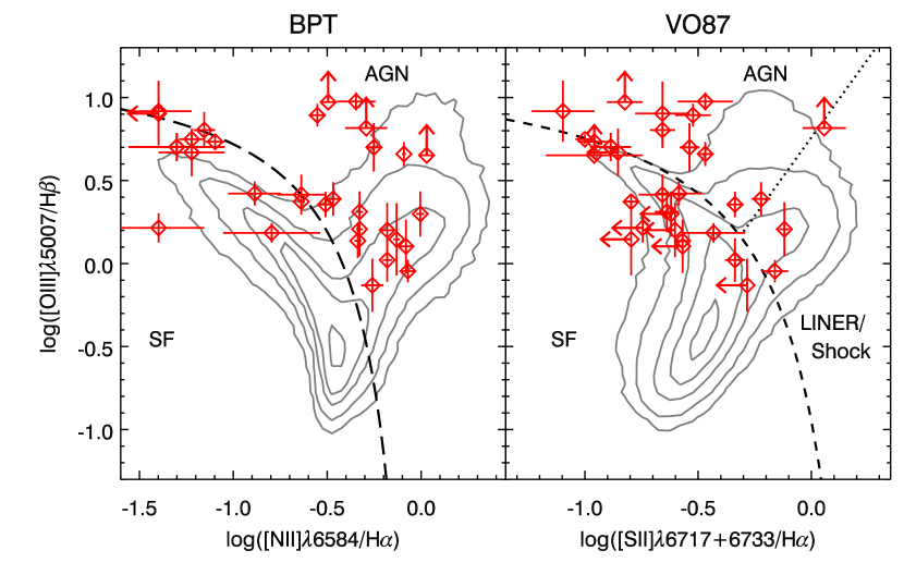
Figure 16: The BPT and VO87 line-ratio diagnostic diagrams for the 33 TKRS2 galaxies with high-confidence ($Q_{M}\geq 3$) redshifts and H$\beta$+[O III] in the $H$ band and H$\alpha$+[N II]+[S II] in the $K$ band. For comparison, a sample of $z\approx 0$ SDSS galaxies are shown as gray contours (drawn from Trump et al., 2015). These TKRS2 $z\approx 2.3$ galaxies generally have higher [O III]/H$\beta$ ratios than $z\approx 0$ galaxies, as noted in previous work (e.g., Trump et al., 2013; Masters et al., 2014; Steidel et al., 2014; Coil et al., 2015).

Figure 16 shows our $z\approx 2.3$ TKRS2 galaxies in the BPT and VO87 diagrams, with a $z<0.1$ sample of SDSS galaxies (drawn from Trump et al., 2015) shown for comparison. We measure rest-frame optical emission lines for our galaxies by subtracting a local linear continuum and fitting each line with a single Gaussian. For placement in the BPT or VO87 diagrams, we require at least one line in each line-ratio pair to be measured at $>1\sigma$: for our targets, this requires [O III] or H$\beta$ to be $>1\sigma$-detected in the $H$-band and [N II] or H$\alpha$ (for the BPT) or [S II] or H$\alpha$ (for the VO87) to be $>1\sigma$-detected in the $K$-band. Figure 16 shows the 33 galaxies in the $1.99<z<2.49$ redshift interval meeting this criterion for BPT and VO87 line ratios. Line ratios with only one line measured at $>1\sigma$ are treated as limits; in our galaxies, this results in [O III]/H$\beta$ lower limits (when H$\beta$ is not well detected) and [N II]/H$\alpha$ or [S II]/H$\alpha$ upper limits (when [N II] or [S II] is not well detected).

As observed in previous work (e.g., Erb et al., 2008; Trump et al., 2011; Juneau et al., 2014; Coil et al., 2015), we find that our $z\approx 2.3$ targets tend to have higher [O III]/H$\beta$ ratios than $z\approx 0$ galaxies at a fixed [N II]/H$\alpha$ ratio. In particular, the $z\approx 2.3$ galaxies tend to lie between the low-metallicity star-forming galaxy locus (upper left of Fig. 16) and the AGN locus (upper right). The $z\approx 2$ galaxies similarly have high [O III]/H$\beta$ ratios in the VO87 diagram, but have a lower fraction of [S II]/H$\alpha$ ratios elevated above the $z\approx 0$ star-forming galaxy population. Masters et al. (2014) similarly noted that $z\approx 2$ emission-line galaxies are more unusual in the BPT diagram than in the VO87 diagram, arguing that this results from higher N/O abundance at high redshift (see also Steidel et al., 2014). One possible mechanism for producing higher N/O abundance is Wolf-Rayet stars, which (if present in sufficient quantities) might also contribute to the higher [Ne III]/[O III] fluxes observed in $z\approx 2$ galaxies (Zeimann et al., 2014). It is not, however, immediately clear why high-redshift H II regions would produce a much larger fraction of Wolf-Rayet stars compared to today. An alternative explanation for the different BPT and VO87 diagram positions of $z\approx 2$ galaxies is that these galaxies host a substantial fraction of weak AGNs with low-metallicity narrow-line regions (NLR) (e.g., Trump et al., 2011), since the [N II]/H$\alpha$ ratio is a much more sensitive metallicity indicator than [S II]/H$\alpha$. The AGN NLR gas is located on $\sim$kpc scales, and so it is quite plausible that it would have the same low metallicities as typical galaxies at $z\approx 2$.

7 Summary

The present survey of the GOODS-North field complements the original Team Keck Redshift Survey (TKRS, Wirth et al., 2004), which obtained optical spectra of galaxies in the same field and helped to establish the DEIMOS spectrograph and the Keck II telescope as the world’s leading combination for visible-wavelength multi-object optical spectroscopy of distant galaxies. Similarly, the TKRS2 program demonstrates the unique capabilities of MOSFIRE and the Keck I telescope to study sizeable samples of galaxies in the near-IR. In the spirit of the original TKRS project, we offer all data products related to the TKRS2 survey — including raw images, data reduction scripts, 2-D reduced spectra, and extracted 1-D spectra — freely to the community to allow researchers access to representative MOSFIRE spectra.

Figure 2: Layout for mask gdn1211_JHK1. Blue envelope indicates the imaging region of MOSFIRE. Large red rectangle indicates region accessible to slits. Individual slits appear as numbered yellow rectangles with corresponding target names as indicated. Small red rectangles indicate mask alignment boxes around stars. Compass rose at top right indicates orientation of the image, and scale bar in lower left indicates angular scale.

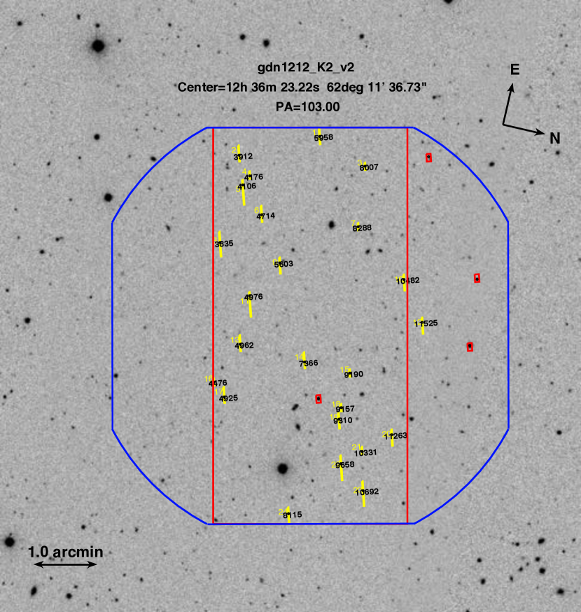
Figure 3: Layout for mask gdn1212_K2; as in Fig. 2.

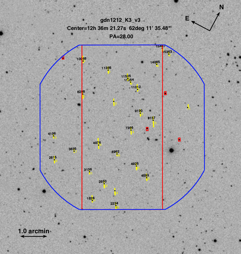
Figure 4: Layout for mask gdn1212_K3; as in Fig. 2.

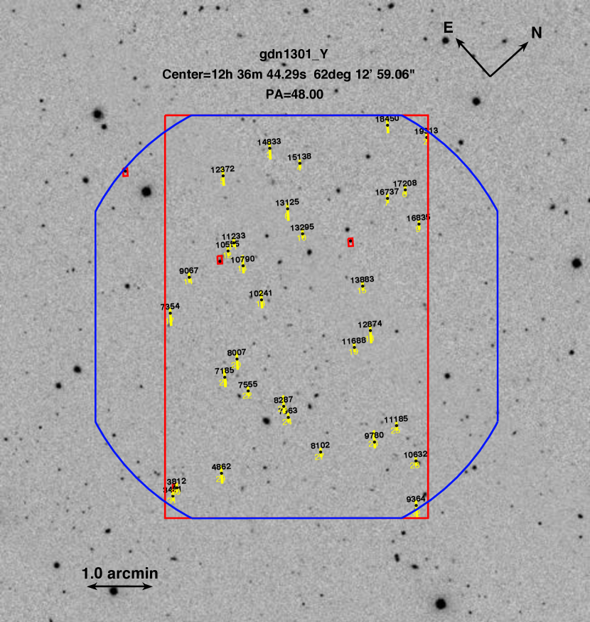
Figure 5: Layout for mask gdn1301_Y; as in Fig. 2.

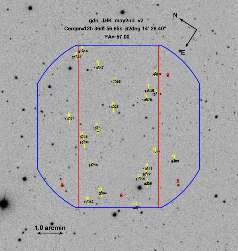
Figure 6: Layout for mask gdn_JHK_may2nd; as in Fig. 2.

Figure 9: A comparison of the emission line S/N achieved by MOSFIRE and MOIRCS in 1 h. The MOIRCS H$\alpha$ line fluxes and errors are taken from Table 3 of Yoshikawa et al. (2010). MOSFIRE achieves $\sim$2–3 times higher S/N as MOIRCS in the same exposure time, with some scatter due to presence of of telluric features in some spectra.

Figure 10: The sensitivity of MOSFIRE for line detection in 1 h in the four $YJHK$ filters. The flux limit is characterized for a fiducial H$\alpha$ emission line of rest-frame width $\sigma_{0}=85~{}\mathrm{km~{}s}^{-1}$ at the $3\sigma$ level, as a function of wavelength of the line peak. We flux calibrated spectra using HST/WFC3 slitless grism observations of a subset of $z\approx 1.5$ galaxies, and so implicitly included a correction for the average slit losses. The 1 h $3\sigma$ flux limit of MOSFIRE is $\sim 1\times 10^{-17}\mathrm{~{}erg~{}s}^{-1}\mathrm{~{}cm}^{-2}$ in regions with no sky lines in the $YJH$ filters, and $\sim$4–$6\times 10^{-17}\mathrm{~{}erg~{}s}^{-1}\mathrm{~{}cm}^{-2}$ in the $K$ filter.

Figure 14: Illustration of our survey strategy to observe selected targets at multiple position angles. The figure shows a ground-based $K$-band image of object 4925, an emission-line galaxy at $z=2.245$. Superimposed on this image are the projected sky locations of the MOSFIRE slit at three position angles, corresponding to three of our mask designs.

Table 1: Observation parameters

						Exposure time
		$\alpha$	$\delta$	P.A.		$Y$	$J$	$H$	$K$
Mask Number	Mask Name	(J2000)	(J2000)	($\arcdeg$)	$N_{t}$	(h)	(h)	(h)	(h)
1	gdn1211_JHK1	12:36:21.58	+62:11:33.23	$-25.5$	25	$\cdots$	1.0	1.0	1.0
2	gdn1212_K2	12:36:23.18	+62:11:36.73	103.0	24	$\cdots$	$\cdots$	$\cdots$	2.0
3	gdn1212_K3	12:36:21.27	+62:11:35.48	28.0	26	$\cdots$	$\cdots$	$\cdots$	1.5
4	gdn1301_Y	12:36:49.93	+62:13:58.06	43.0	32	1.0	$\cdots$	$\cdots$	$\cdots$
5	gdn_JHK_may2nd	12:36:56.73	+62:14:27.40	$-55.0$	24	$\cdots$	1.0	2.0	3.0

Table 2: Redshift quality distribution

Quality Code	Definition	Number	Fraction
4	Very secure redshift ($P>99\%$)	56	0.58
3	Secure redshift ($P>95\%$)	2	0.02
2.5	Degenerate redshift, but matches $z_{\mathrm{phot}}$	8	0.08
2	Degenerate redshift, does not match $z_{\mathrm{phot}}$	4	0.04
1	Highly uncertain redshift	7	0.07
0	No redshift	20	0.21

Table 3: Redshift catalog

	$\alpha$	$\delta$							$t_{\mathrm{exp}}$
ID	(J2000)	(J2000)	Class	$m_{\mathrm{F160W}}$	prior $z_{\mathrm{spec}}$	$z_{\mathrm{spec}}$ source	$z_{\mathrm{phot}}$	Filters	(h)	$N_{\mathrm{PA}}$	$z_{M}$	$Q_{M}$	Spectral Features
(1)	(2)	(3)	(4)	(5)	(6)	(7)	(8)	(9)	(10)	(11)	(12)	(13)	(14)
1576	189.10121960	62.14110330	moircs	22.45	$\cdots$	$\cdots$	2.00	JHK	3.0	1	1.998	4.0	hb,o3
1826	189.07826120	62.14436230	emline	23.21	$\cdots$	$\cdots$	2.36	K	1.5	1	2.302	4.0	ha,n2,s2
2234	189.04746530	62.14840220	emline	22.32	$\cdots$	$\cdots$	2.30	K	1.5	1	$\cdots$	0.0	$\cdots$
2815	189.14816630	62.15564680	emline	23.47	$\cdots$	$\cdots$	2.36	JHK	4.5	2	2.362	4.0	o2,ha,n2
2930	189.07478850	62.15701200	emline	23.69	$\cdots$	$\cdots$	2.11	K	1.5	1	$\cdots$	0.0	$\cdots$
2960	189.12710660	62.15744680	emline	23.67	$\cdots$	$\cdots$	2.31	JHK	3.0	1	2.311	4.0	o3
3136	189.09941700	62.15932020	emline	24.32	$\cdots$	$\cdots$	1.97	K	1.5	1	$\cdots$	0.0	$\cdots$
3450	189.12699890	62.16260147	emline	23.45	2.086	Reddy06	2.09	JHK	3.0	1	2.088	4.0	hb,o3
3461	189.15730650	62.16280760	emline	23.29	0.512	Barger08	0.51	Y	1.0	1	0.513	4.0	ha,s2
3812	189.15918530	62.16485290	emline	20.80	0.512	Wirth04	0.51	Y	1.0	1	0.513	4.0	ha,n2,s2
3835	189.13033780	62.16611130	emline	23.37	$\cdots$	$\cdots$	2.32	JHK	6.5	3	2.302	4.0	o2,ha,n2,s2
3912	189.17999268	62.16590118	emline	21.82	3.661	Reddy06	3.68	K	2.0	1	2.370	4.0	o3
4098	189.09874990	62.16919680	emline	23.32	$\cdots$	$\cdots$	2.61	JHK	3.0	1	2.174	2.0	ha
4106	189.16402480	62.16850060	moircs	22.25	$\cdots$	$\cdots$	2.34	JHK	6.5	3	2.352	4.0	o2,ha,n2,s2
4176	189.16975470	62.16971020	emline	22.87	$\cdots$	$\cdots$	2.30	K	2.0	1	2.276	2.5	ha
4476	189.05470460	62.17253080	emline	23.88	2.236	Reddy06	2.12	K	2.0	1	2.243	4.0	ha,n2
4593	189.02857620	62.17261300	emline	21.62	2.509	Reddy06	2.37	K	1.5	1	2.321	4.0	ha,n2
4714	189.15032350	62.17497220	emline	23.17	$\cdots$	$\cdots$	2.31	JHK	5.0	2	2.307	4.0	ha,o2
4862	189.14878440	62.17573170	quiescent	21.65	$\cdots$	$\cdots$	1.26	Y	1.0	1	$\cdots$	0.0	$\cdots$
4925	189.04794490	62.17603260	moircs	23.94	$\cdots$	$\cdots$	2.09	JHK	6.5	3	2.245	4.0	ha,n2,s2
4962	189.07818880	62.17702260	emline	23.79	2.322	Reddy06	2.48	JHK	6.5	3	2.265	4.0	o2,ha,n2,s2
4976	189.10537690	62.17655430	moircs	22.22	$\cdots$	$\cdots$	2.09	JHK	6.5	3	2.084	4.0	ha,n2,s2
5161	189.15475520	62.17891140	emline	25.43	$\cdots$	$\cdots$	2.64	JHK	3.0	1	$\cdots$	0.0	$\cdots$
5603	189.12673430	62.18227440	emline	24.00	$\cdots$	$\cdots$	2.38	K	2.0	1	2.089	2.5	ha
5958	189.19959020	62.18498830	emline	24.75	2.349	Reddy06	0.14	K	2.0	1	2.346	3.0	ha,n2
7185	189.18647840	62.19263560	quiescent	24.60	$\cdots$	$\cdots$	0.65	Y	1.0	1	$\cdots$	0.0	$\cdots$
7354	189.23179980	62.19318350	emline	22.38	0.558	Wirth04	0.56	Y	1.0	1	0.559	4.0	ha
7366	189.07653870	62.19417900	moircs	23.17	2.390	Reddy06	2.62	JHK	6.5	3	2.398	4.0	o2,ha,n2
7417	189.09559120	62.19458080	emline	23.91	$\cdots$	$\cdots$	2.40	JHK	3.0	1	$\cdots$	0.0	$\cdots$
7555	189.17220320	62.19468670	emline	21.43	0.585	Barger08	0.59	Y	1.0	1	0.585	4.0	ha,n2,s2
7930	189.06017860	62.19777610	emline	23.16	2.221	Reddy06	2.43	JHK	3.0	1	2.227	4.0	ha
7963	189.14699090	62.19774920	quiescent	22.57	1.223	Barger08	1.21	Y	1.0	1	$\cdots$	0.0	$\cdots$
8007	189.18925060	62.19811130	emline	23.00	$\cdots$	$\cdots$	2.81	K	2.0	1	2.141	2.0	ha?
8102	189.12134530	62.19809840	emline	22.60	0.529	Wirth04	0.53	Y	1.0	1	0.530	4.0	ha,n2
8115	188.99305430	62.19879980	emline	23.88	$\cdots$	$\cdots$	2.28	K	2.0	1	$\cdots$	0.0	$\cdots$
8287	189.15315580	62.19891510	emline	20.73	0.557	Ferreras09	0.56	Y	1.0	1	0.556	4.0	ha,n2
8288	189.15584380	62.19987360	emline	23.62	$\cdots$	$\cdots$	2.31	K	3.5	2	2.103	1.0	ha?
8489	189.23250720	62.20029800	emline	22.39	2.737	Barger08	1.86	JHK	6.0	1	2.017	4.0	ha,n2,s2
8974	189.31296290	62.20461920	emline	23.34	$\cdots$	$\cdots$	2.49	JHK	6.0	1	$\cdots$	0.0	$\cdots$
9067	189.23950180	62.20293930	emline	19.80	0.664	Ferreras09	0.66	Y	1.0	1	0.670	1.0	ha?
9157	189.05649000	62.20599320	emline	23.20	2.437	Reddy06	2.45	JHK	6.5	3	2.441	4.0	o2,ne3,ha,n2,s2
9190	189.07614090	62.20616030	emline	23.61	2.441	Reddy06	2.49	JHK	6.5	3	2.439	4.0	ha,n2
9310	189.05000530	62.20607770	emline	23.38	$\cdots$	$\cdots$	2.55	K	2.0	1	2.434	4.0	ha,n2
9338	189.27751870	62.20708550	emline	23.74	2.443	Reddy06	2.38	JHK	6.0	1	2.445	4.0	ha
9364	189.06492560	62.20691180	quiescent	21.82	$\cdots$	$\cdots$	1.00	Y	1.0	1	$\cdots$	0.0	$\cdots$
9658	189.02636730	62.20912420	emline	23.01	$\cdots$	$\cdots$	2.18	JHK	5.0	2	2.487	4.0	o2,ha,n2
9772	189.26833810	62.21060800	emline	26.02	$\cdots$	$\cdots$	1.93	JHK	6.0	1	1.956	4.0	ha,n2,s2
9780	189.10558960	62.20981490	emline	21.60	0.533	Barger08	0.50	Y	1.0	1	0.532	1.0	ha
10113	189.26084480	62.21222410	emline	22.96	$\cdots$	$\cdots$	2.43	JHK	6.0	1	2.421	4.0	ha,n2
10230	189.27795300	62.21239100	emline	22.17	$\cdots$	$\cdots$	2.37	JHK	6.0	1	2.212	2.5	ha
10241	189.20414020	62.21275500	emline	23.46	0.512	Barger08	0.51	Y	1.0	1	0.682	1.0	ha
10331	189.03548710	62.21373890	emline	24.31	$\cdots$	$\cdots$	2.11	JHK	5.0	2	2.241	2.5	ha
10482	189.13310980	62.21439890	emline	23.07	2.443	Reddy06	2.47	K	2.0	1	2.444	4.0	ha
10555	189.23622490	62.21462030	quiescent	21.58	1.234	Wirth04	1.24	Y	1.0	1	1.235	4.0	hb,o3
10632	189.08267550	62.21434780	emline	20.33	0.694	Wirth04	0.71	Y	1.0	1	0.627	2.0	ha
10692	189.01454620	62.21620650	emline	23.94	$\cdots$	$\cdots$	2.51	JHK	5.0	2	2.491	2.5	ha,o2
10790	189.22455130	62.21502430	emline	19.84	0.641	Wirth04	0.64	Y	1.0	1	0.642	4.0	ha,n2
10968	189.17571390	62.21808980	emline	23.88	$\cdots$	$\cdots$	2.04	K	1.5	1	2.572	2.0	ha?
11012	189.09411750	62.21837350	emline	23.55	2.981	Reddy06	2.77	K	1.5	1	2.990	4.0	hb,o3
11185	189.10440320	62.21683960	emline	19.52	0.518	Wirth04	0.52	Y	1.0	1	$\cdots$	0.0	$\cdots$
11233	189.23715020	62.21713110	quiescent	20.99	1.010	Ferreras09	1.24	Y	1.0	1	1.049	1.0	o3?
11263	189.04815160	62.22022640	emline	22.80	$\cdots$	$\cdots$	2.16	JHK	5.0	2	2.492	2.5	ha
11264	189.10681730	62.22033690	emline	24.40	$\cdots$	$\cdots$	2.51	K	1.5	1	2.442	2.5	ha
11385	189.14063940	62.22037180	emline	23.26	$\cdots$	$\cdots$	2.34	K	1.5	1	$\cdots$	0.0	$\cdots$
11525	189.11224190	62.22162740	moircs	23.73	$\cdots$	$\cdots$	0.54	JHK	6.5	3	2.398	4.0	ha,n2,s2
11688	189.15119800	62.22218150	emline	22.14	0.679	Wirth04	0.68	Y	1.0	1	0.680	4.0	ha
12369	189.32200623	62.22800064	emline	27.55	$\cdots$	$\cdots$	0.30	JHK	6.0	1	2.985	2.0	o3
12372	189.26808890	62.22644260	quiescent	20.84	1.242	Barger08	1.24	Y	1.0	1	1.238	3.0	hb,o3?
12874	189.15210960	62.22802410	emline	20.12	0.556	Wirth04	0.56	Y	1.0	1	0.557	4.0	ha,n2
12962	189.34192260	62.23206070	emline	26.98	$\cdots$	$\cdots$	0.95	JHK	6.0	1	$\cdots$	0.0	$\cdots$
13174	189.17022100	62.23287270	emline	23.71	3.087	Reddy06	2.91	JHK	6.0	1	2.990	4.0	hb,o3
13230	189.03771860	62.23306260	emline	22.96	2.048	Reddy06	2.07	JHK	3.0	1	2.048	4.0	o3
13295	189.21578180	62.23163490	emline	20.01	0.556	Wirth04	0.56	Y	1.0	1	0.557	4.0	ha,n2,s2
13678	189.18366540	62.23613790	emline	23.92	2.273	Reddy06	2.31	JHK	6.0	1	2.273	4.0	ha
13883	189.17278880	62.23411310	emline	19.75	0.555	Ferreras09	0.55	Y	1.0	1	$\cdots$	0.0	$\cdots$
14025	189.17174480	62.23797870	emline	23.08	$\cdots$	$\cdots$	2.03	JHK	6.0	1	1.989	4.0	ha,n2
14085	189.08706410	62.23762110	emline	22.22	$\cdots$	$\cdots$	1.94	JHK	4.5	2	2.092	4.0	o3,ha,n2,s2
14428	189.14829020	62.24000410	emline	21.25	2.005	Reddy06	1.85	JHK	6.0	1	2.015	4.0	ha,n2,s2
14620	189.29724600	62.24215960	emline	24.29	$\cdots$	$\cdots$	1.43	JHK	6.0	1	2.188	4.0	ha,n2
14833	189.26218500	62.23988580	emline	19.39	0.511	Wirth04	0.51	Y	1.0	1	0.512	4.0	ha,n2
15138	189.24516100	62.24303100	emline	19.58	0.676	Wirth04	0.68	Y	1.0	1	0.678	4.0	ha,n2
15363	189.07931690	62.24679590	emline	22.78	$\cdots$	$\cdots$	2.36	K	1.5	1	2.307	4.0	ha,n2,s2
15497	189.09058260	62.24801280	moircs	22.97	2.204	Reddy06	2.40	JHK	4.5	2	2.207	4.0	o2,ha,n2
16028	189.21590160	62.25131100	emline	23.23	$\cdots$	$\cdots$	2.19	JHK	6.0	1	2.194	4.0	ha,n2
16260	189.25190810	62.25246110	emline	22.58	$\cdots$	$\cdots$	2.33	JHK	6.0	1	2.330	4.0	ha,n2
16616	189.27755100	62.25461080	emline	23.35	$\cdots$	$\cdots$	2.23	JHK	6.0	1	2.188	1.0	ha?
16737	189.19911340	62.25358100	emline	20.95	0.533	Wirth04	0.52	Y	1.0	1	0.534	4.0	ha,n2
16835	189.17730510	62.25515580	emline	21.47	0.533	Wirth04	0.53	Y	1.0	1	0.533	4.0	ha,n2,s2
16938	189.27283970	62.25734420	emline	23.46	$\cdots$	$\cdots$	2.08	JHK	6.0	1	$\cdots$	0.0	$\cdots$
17088	189.18602430	62.25877660	emline	22.50	2.453	Barger08	2.34	JHK	6.0	1	2.273	4.0	ha,n2,s2
17208	189.19601500	62.25835770	emline	22.71	0.570	Wirth04	0.57	Y	1.0	1	0.571	4.0	ha
18450	189.22856060	62.26592220	emline	21.33	0.504	Barger08	0.51	Y	1.0	1	0.606	1.0	ha?
19074	189.26210950	62.27037430	emline	23.11	$\cdots$	$\cdots$	2.31	JHK	6.0	1	$\cdots$	0.0	$\cdots$
19313	189.20938530	62.27120450	emline	21.59	0.502	Ferreras09	0.50	Y	1.0	1	$\cdots$	0.0	$\cdots$
19547	189.18296560	62.27247100	emline	21.87	$\cdots$	$\cdots$	2.36	JHK	6.0	1	2.320	4.0	ha,n2
21414	189.17590600	62.28647920	emline	22.71	$\cdots$	$\cdots$	2.62	JHK	6.0	1	$\cdots$	0.0	$\cdots$
21581	189.18680050	62.28775230	emline	22.50	2.032	Reddy06	2.09	JHK	6.0	1	$\cdots$	0.0	$\cdots$

Note. — (1) Object identifier in CANDELS catalog. (2) Right ascension of the target, in decimal degrees. (3) Declination of the target, in decimal degrees. (4) The sample class to which the target belongs, as described in §3. (5) The apparent AB magnitude of the target in the F160W passband (Koekemoer et al., 2011) as measured from CANDELS HST WFC3 imagery. (6) The presumed redshift of the target from previous spectroscopic surveys (when available). (7) The source of the presumed redshift. (8) The estimated redshift of the source derived via multiband photometry from the CANDELS survey. (9) The list of MOSFIRE passbands in which we observed the target. (10) The total MOSFIRE exposure time devoted to the target. (11) The number of different position angles at which we observed the target. (12) The redshift derived from MOSFIRE spectroscopy. (13) The redshift quality code, $Q_{M}$, as described in §4.3. (14) The identification of specific spectral features on which we based the redshift measurement, where ha=H$\alpha$, hb=H$\beta$, n2=[N II], ne3=[Ne III], o2=[O II], o3=[O III], s2=[S II], and question marks indicate marginally-detected lines.

References

- Baldwin, Phillips & Terlevich (1981) Baldwin, J. A., Phillips, M. M. & Terlevich, R. 1981, PASP, 93, 5
- Barger et al. (2008) Barger, A. J., Cowie, L. L., & Wang, W.-H. 2008, ApJ, 689, 687
- Brammer et al. (2012) Brammer, G. B., Sánchez-Janssen, R., Labbé, I. et al. 2012, ApJS, 200, 13
- Brinchmann, Pettini & Charlot (2008) Brinchmann, J., Pettini, M. & Charlot, S. 2008, MNRAS, 385, 769
- Coil et al. (2015) Coil, A. L., Aird, J., Reddy, N. et al. 2015, ApJ, 801, 35
- Cooper et al. (2011) Cooper, M. C., Aird, J. A., Coil, A. L. et al. 2011, ApJS, 193, 14
- Cowie, Hu & Songaila (1995) Cowie, L. L., Hu, E. M., Songaila, A. 1995, AJ, 110, 1576
- Dahlen et al. (2013) Dahlen, T., Mobasher, B., Faber, S. M. et al. 2013, ApJ, 775, 93
- Elmegreen, Elmegreen & Hirst (2004) Elmegreen, D. M., Elmegreen, B. G. & Hirst, A. C. 2004, ApJ, 604, 21
- Erb et al. (2008) Erb, D. K., Shapley, A. E., Pettini, M., Steidel, C. C., Reddy, N. A. & Adelberger, K. L. 2006, ApJ, 644, 813
- Ferreras et al. (2009) Ferreras, I., Pasquali, A., Malhotra, S. et al. 2009, ApJ, 706, 158
- Galametz et al. (2013) Galametz, A., Grazian, A., Fontana, A. et al. 2013, ApJS, 206, 10
- Giavalisco et al. (2004) Giavalisco, M., Ferguson, H. C., Koekemoer, A. M., et al. 2004, ApJ, 600, L93
- Grogin et al. (2011) Grogin, N. A., Kocevski, D. D., Faber, S. M. et al.2011, ApJS, 197, 35
- Guo et al. (2012) Guo, Y., Giavalisco, M., Ferguson, H. C., Cassata, P. & Koekemoer, A. M. 2012, ApJ, 757, 120
- Guo et al. (2013) Guo, Y., Ferguson, H. C., Giavalisco, M. et al. 2013, ApJS, 207, 24
- Guo et al. (2015) Guo, Y., Ferguson, H. C., Bell, E. F., et al. 2015, ApJ, 800, 39
- Juneau et al. (2014) Juneau, S., Bournaud, F., Charlot, S. et al.2014, ApJ, 788, 88
- Kassin et al. (2012) Kassin, S. A., Weiner, B. J., Faber, S. M. et al. 2012, ApJ, 758, 106
- Kashino et al. (2013) Kashino, D., Silverman, J. D., Rodighiero, G. et al. 2013, ApJ, 777, 8
- Kassis et al. (2012) Kassis, M., Wirth, G. D., Phillips, A. C., & Steidel, C. C. 2012, Proc. SPIE, 8448, 844807
- Kauffmann et al. (2003) Kauffmann, G., Heckman, T. M., Tremonti, C. et al. 2003b, MNRAS, 346, 1055
- Kennicutt (1998) Kennicutt, R. C., Jr. 1998, ARA&A, 36, 189
- Kewley et al. (2001) Kewley, L. J., Dopita, M. A., Sutherland, R. S., Heisler, C. A. & Trevena, J. 2001, ApJ, 556, 121
- Kewley et al. (2006) Kewley, L. J., Groves, B., Kauffmann, G. & Heckman, T. 2006, MNRAS, 372, 961
- Kewley et al. (2013) Kewley, L. J., Maier, C., Yabe, K., Ohta, K., Akiyama, M., Dopita, M. A. & Yuan, T. 2013, MNRAS, 774, 100
- Koekemoer et al. (2011) Koekemoer, A. M., Faber, S. M., Ferguson, H. C. et al. 2011, ApJS, 197, 36
- Kriek et al. (2015) Kriek, M., Shapley, A. E., Reddy, N. A. et al.2015, ApJS submitted (arXiv:1412.1835)
- Liu et al. (2008) Liu, X., Shapley, A. E., Coil, A. L., Brinchmann, J. & Ma, C.-P. 2008, ApJ, 678, 758
- Madau & Dickinson (2014) Madau, P. & Dickinson, M. 2014, ARA&A, 52, 415
- Masters & Capak (2011) Masters, D. & Capak, P. 2011, PASP, 123, 638
- Masters et al. (2014) Masters, D., McCarthy, P., Siana, B. et al. 2014, ApJ, 785, 153
- McLean et al. (2012) McLean, I. S., Steidel, C. C., Epps, H. W., et al. 2012, Proc. SPIE, 8446, 84460J
- Papovich et al. (2005) Papovich, C., Dickinson, M., Giavalisco, M., Conselice, C. J., & Ferguson, H. C. 2005, ApJ, 631, 101
- Pérez-González et al. (2013) Pérez-González, P. G., Cava, A., Barro, G. et al. 2013, ApJ, 762, 46
- Reddy et al. (2006) Reddy, N. A., Steidel, C. C., Erb, D. K., Shapley, A. E. & Pettini, M. 2006, ApJ, 653, 1004
- Steidel et al. (2014) Steidel, C. C., Rudie, G. C., Strom, A. L. et al. 2014, ApJ, 795, 165
- Trump et al. (2011) Trump, J. R., Weiner, B. J., Scarlata, C. et al. 2011, ApJ, 743, 144
- Trump et al. (2013) Trump, J. R., Konidaris, N. P., Barro, G., et al. 2013, ApJ, 763, L6
- Trump et al. (2015) Trump, J. R., Sun, M., Zeimann, G. R. et al. 2015, ApJsubmitted (arXiv:1501.02801)
- Veilleux & Osterbrock (1987) Veilleux, S. & Osterbrock, D. E. 1987, ApJS, 63, 295
- Vernet et al. (2011) Vernet, J., Dekker, H., D’Odorico, S., et al. 2011, A&A, 536, A105
- Williams et al. (2009) Williams, R. J., Quadri, R. F., Franx, M., van Dokkum, P. & Labbé, I. 2009, ApJ, 691, 1879
- Wirth et al. (2004) Wirth, G. D., Willmer, C. N. A., Amico, P. et al. 2004, AJ, 127, 3121
- Wisnioski et al. (2015) Wisnioski, E., Förster Schreiber, N. M., Wuyts, S. et al. 2015 ApJ, 799, 209
- Wright et al. (2010) Wright, S. A., Larkin, J. E., Graham, J. R. & Ma, C.-P. 2010, ApJ, 711, 1291
- York et al. (2000) York, D. G. et al. 2000, AJ, 120, 1579
- Yoshikawa et al. (2010) Yoshikawa, T., Akiyama, M., Kajisawa, M., et al. 2010, ApJ, 718, 112
- Zeimann et al. (2014) Zeimann, G. R., Ciardullo, R., Gebhardt, H. et al. 2015, ApJ, 798, 29