Bayesian inference on the sphere beyond statistical isotropy

Abstract

We present a general method for Bayesian inference of the underlying covariance structure of random fields on a sphere. We employ the Bipolar Spherical Harmonic (BipoSH) representation of general covariance structure on the sphere. We illustrate the efficacy of the method as a principled approach to assess violation of statistical isotropy (SI) in the sky maps of Cosmic Microwave Background (CMB) fluctuations. SI violation in observed CMB maps arise due to known physical effects such as Doppler boost and weak lensing; yet unknown theoretical possibilities like cosmic topology and subtle violations of the cosmological principle, as well as, expected observational artefacts of scanning the sky with a non-circular beam, masking, foreground residuals, anisotropic noise, etc. We explicitly demonstrate the recovery of the input SI violation signals with their full statistics in simulated CMB maps. Our formalism easily adapts to exploring parametric physical models with non-SI covariance, as we illustrate for the inference of the parameters of a Doppler boosted sky map. Our approach promises to provide a robust quantitative evaluation of the evidence for SI violation related anomalies in the CMB sky by estimating the BipoSH spectra along with their complete posterior.

1 Introduction

Many astronomical measurements on sky, as well as, data from other other parts of science, such as, geophysical and environmental modelling on the globe, deal with analysis of random fields on a sphere. Advancement in observational data has opened up the possibility of posing deeper inference problems with sophisticated analysis tools. In this paper we present a novel way to implement Bayesian inference of the underlying covariance structure. We develop our analysis strongly motivated by the analysis of cosmic microwave background (CMB) sky maps to infer the statistical isotropy (SI) of our observed universe. However, the methodology is applicable to Bayesian inference for other cosmological studies, and more widely to any study involving a scalar random field on the sphere.

For a statistically isotropic Gaussian random field, the two-point correlation function is rotationally invariant and hence the covariance matrix of the corresponding random spherical harmonic coefficients, i.e., $\left\langle a_{lm}^{*}a_{l^{\prime}m^{\prime}}\right\rangle$ is diagonal and independent of the azimuthal multipole index $m$. Therefore, the angular power spectrum ($C_{l}=\left\langle a_{lm}^{*}a_{lm}\right\rangle$) can alone provide a complete statistical representation of the field on the sphere. However, in presence of SI violation, the covariance matrix $\left\langle a_{lm}^{*}a_{l^{\prime}m^{\prime}}\right\rangle$ can depend on $m$ and the off-diagonal components can be nonzero. This calls for a representation of the random field that generalizes the angular power spectrum. Bipolar Spherical harmonic representation (BipoSH) was first proposed by Hajian and Souradeep [1] to analyze SI violation signals on CMB. Any SI violation of a random field on a sphere can be completely represented in BipoSH spectra ($\tilde{A}_{ll^{\prime}}^{LM}$) [2, 3, 4, 5]. The $L=0$ component of the BipoSH spectra, $\tilde{A}_{ll}^{00}$, is the angular power spectrum, $C_{l}$.

The angular power spectrum $(C_{l})$ can be estimated from the observed sky map using Bayesian statistics. Earlier Maximum likelihood methods [6, 7, 8, 9, 10] were used for optimal estimation of the CMB power spectrum. A straight forward minimisation of the likelihood is computationally prohibitive as it require $O(N_{pix}^{3})$ computational complexity, where $N_{pix}$ is the number of pixels present in the map. Last maximum likelihood methods on CMB dataset were used in some parts of the Boomerang and Maxima datasets. Since $N_{pix}$ increased in the modern experiments, maximum likelihood methods are not a viable option and pseudo-$C_{l}$ methods [11, 12, 13] are used since then. We can explore the full posterior distribution with Monte Carlo sampling. However, this approach relies of the availability of an efficient sampling method. At low multipoles where the posterior of the $C_{l}$ are highly non-Gaussian due to the small number of degrees of freedom, Gibbs sampling [10] is now standard. Other sampling methods, used for sampling the posterior of the CMB power spectrum, involves methods like Hamiltonian Monte Carlo [14] etc.

For a SI violated Gaussian random field on a sphere, calculating the only the angular power spectrum by minimising the likelihood with respect to $C_{l}$ is not sufficient. Although, when the SI violation is small in comparison to the $C_{l}$, the posterior distribution of the $C_{l}$ may not alter significantly, it is still important to minimise the likelihood with respect to the off-diagonal components of the covariance matrix (represented in terms of BipoSH spectra, $\tilde{A}_{ll^{\prime}}^{LM}$), which not only guarantees complete posterior statistics of $C_{l}$ but also provides a complete posterior statistics of BipoSH spectra. We present a novel method for estimating the posterior distribution of BipoSH spectra by sampling the full covariance matrix. The Bayesian method for finding the posterior distribution of BipoSH spectra allows a complete and reliable statistical inference of the presence of SI violation over the sphere. For sampling the posterior, we choose the Hamiltonian Monte Carlo [15, 16, 14], a Monte Carlo method that uses the classical Hamiltonian mechanics for calculating the posterior distribution and is capable of sampling the posterior distribution faster than other conventional MCMC methods in such high dimensional problems.

There has been a phenomenal improvement in CMB observations in the past few years. After recent data release of WMAP-9 and Planck, the observations in CMB have achieved the level of reliability where every single significant departure from the standard model cosmology may present a challenge to our understanding of the universe. The standard homogeneous and isotropic cosmological model dictates that the temperature fluctuation in CMB sky respect Statistical isotropy (SI). However, recent data from Planck hint at some putative signals of SI violation in the CMB sky [17, 18, 19]. There are several theoretical models proposed in literature that lead to SI violation in the CMB such as the non-trivial cosmic topology [20, 6, 21, 22], anisotropic cosmology, etc. [23, 24]. Weak lensing of CMB and Doppler boost are among the known effects that lead to SI violation in the observed CMB [25, 26]. Artefacts of observational reality such as anisotropic noise, foreground residuals from inadequate cleaning, effect of non-circular beam response function, etc. [2, 3, 4] may also yield similar SI violation. Therefore, it is necessary to extract the SI violation signal from observational data accounting for any false signal of observational systematics, and then carefully statistically assess its significance vis a vis peculiarity of a particular realisation of SI covariance. We apply our method of the Bayesian inference of random fields on sphere to analyse simulated CMB maps and recover input isotropy violation signals in the simulated CMB sky. Our method is shown to successfully recover the input signal properly up to high multipoles. Another important fact is that our Bayesian approach produces inferences that are data-dependent; i.e. they allow testing the relative probability of different models given the realized data set. This is in contrast to frequentist approaches that compare the data set to an ensemble of alternate data sets generated from the null hypothesis.

The paper is organised as follows. In section 2, we provide a brief review of the BipoSH formalism and present the likelihood for the full covariance matrix. Section 3 discusses the details of the equation of motion for the HMC method. In section 4, we provide details of our handling of the computational issues. The analysis of simulated CMB sky maps and results are included in the section 5 of the paper. Here, first we do our analysis on statistically isotropic CMB maps and show that recovered BipoSH spectra are consistent with $0$. Then we show our analysis on SI violated sky maps originated from WMAP beam and scan pattern, dipolar modulation and the Doppler boost signal originated from the motion of our galaxy respectively. In this section, we also develop and method to explicitly recover the Doppler boost signal by directly sampling the posterior. The final section 6 is devoted to discussions and conclusions.

2 A brief review of BipoSH representation

Consider measurements that are a linear transform of a random signal and an additive instrumental noise, all being fields defined on a sphere. We pose the general problem of Bayesian inference of the underlying covariance structure of the signal field, given the knowledge of the noise covariance and the linear transformation relating the measured data to the signal.

With no loss of any generality of the problem, we specifically consider the measurement of CMB temperature fluctuations in the sky. The observed sky map is a convolution of the real sky temperature with the instrumental beam with an addition of instrumental noise. Therefore, $\tilde{T}(\gamma)$ the actual temperature signal of the CMB sky along the direction $\gamma$ is linearly related to the observed sky temperature, $\tilde{d}(\gamma)$, as

$$\tilde{d}(\gamma)=\int B(\gamma,\gamma^{\prime})\tilde{T}(\gamma^{\prime})d\Omega_{\gamma^{\prime}}+\tilde{N}(\gamma)\,,$$ (2.1)

where $B(\gamma,\gamma^{\prime})$ is the instrumental beam profile and $\tilde{N}(\gamma)$ is the instrumental noise. For a perfectly circular beam profile, $B(\gamma,\gamma^{\prime})\equiv B(\gamma\cdot\gamma^{\prime})$, assumed in this work, it is easy to deconvolve the effect of the beam after inferring the power spectra. However, if the beam is not circular symmetric then the effect of the beam depends on the full scan pattern of the experiment and its deconvolution may be non-trivial [3, 4, 27, 28, 29].

For data defined on a sphere, it is convenient to work in the spherical harmonic space. The CMB signal, $\tilde{T}(\gamma)$, then can be expanded in terms of spherical harmonics as

$$\tilde{T}(\gamma)=\sum_{l=0}^{\infty}\sum_{m=-l}^{l}a_{lm}Y_{lm}(\gamma)\,,$$ (2.2)

where $Y_{lm}(\gamma)$ are the spherical harmonic functions and $a_{lm}$ are the coefficients in the spherical harmonic basis. Similarly, the observed data, $\tilde{d}(\gamma)$, can also be expanded in spherical harmonics with coefficients, $d_{lm}$.

For a perfectly statistically isotropic sky, the two point correlation function on sky can be expressed in terms of the angular power spectrum, $C_{l}$, alone as

$$\left\langle a_{lm}a_{l^{\prime}m^{\prime}}^{*}\right\rangle=S_{lml^{\prime}m^{\prime}}=C_{l}\delta_{ll^{\prime}}\delta_{mm^{\prime}}\,.$$ (2.3)

Here $\left\langle\,\ldots\,\right\rangle$ denotes the ensemble average. However, when we allow for CMB to have SI violation, $C_{l}$ does not provide a full description of the covariance matrix. A general covariance matrix can be expanded in the BipoSH representation as

$$\left\langle a_{lm}a_{l^{\prime}m^{\prime}}^{*}\right\rangle=\sum_{m,m^{\prime}}\left(-1\right)^{m^{\prime}}A_{ll^{\prime}}^{LM}\mathcal{C}_{lml^{\prime}-m^{\prime}}^{LM}\,,$$ (2.4)

where $\mathcal{C}_{lml^{\prime}-m^{\prime}}^{LM}$ are the Clebsch Gordon coefficients and $A_{ll^{\prime}}^{LM}$ are the BipoSH spectra that provide a natural generalisation of the angular power spectrum. Since, $\mathcal{C}_{lml^{\prime}-m^{\prime}}^{LM}$ span the entire space of the Covariance matrix, given a set of BipoSH spectra we can calculate the entire covariance matrix and vice versa. It is more convenient for most non-SI phenomena to use the even-parity BipoSH spectra $\bar{A}_{ll^{\prime}}^{LM}=\frac{\sqrt{2L+1}}{\sqrt{2l+1}\sqrt{2l^{\prime}+1}}\frac{1}{\mathcal{C}_{l0l^{\prime}0}^{L0}}A_{ll^{\prime}}^{LM}$ that more closely generalise $C_{l}$. The biposh representation splits the covariance matrix into pieces that transform separately under the action of the group of rotation $SO(3)$. The scalar (rotationally invariant) term is the power spectrum, $C_{l}$.

The goal of this paper is to calculate the posterior distribution of $A_{ll^{\prime}}^{LM}$ from the observed sky map, i.e., $P(A_{ll^{\prime}}^{LM}|d_{lm})$ or $P(S_{lml^{\prime}m^{\prime}}|d_{lm})$. Rather than computing this pdf directly we sample the joint probability distribution, $P(S_{lml^{\prime}m^{\prime}},a_{lm}|d_{lm})$, and then marginalise over $a_{lm}$. The joint distribution can be obtained directly by using Bayes Theorem [6, 30, 31, 8]

$$P(S_{lml^{\prime}m^{\prime}},a_{lm}|d_{lm}) = P(d_{lm}|a_{lm})P(a_{lm}|S_{lml^{\prime}m^{\prime}})P(S_{lml^{\prime}m^{\prime}})$$ (2.5)

$$= \frac{1}{\sqrt{|N_{lml^{\prime}m^{\prime}}|}}\exp\left[-\frac{1}{2}\sum_{lml^{\prime}m^{\prime}}\left(d_{lm}^{*}-a_{lm}^{*}\right)^{T}N_{lml^{\prime}m^{\prime}}^{-1}\left(d_{l^{\prime}m^{\prime}}-a_{l^{\prime}m^{\prime}}\right)\right]$$

$$\times\frac{1}{\sqrt{|S_{lml^{\prime}m^{\prime}}|}}\exp\left(-\frac{1}{2}\sum_{lml^{\prime}m^{\prime}}a_{lm}^{*T}S_{lml^{\prime}m^{\prime}}^{-1}a_{l^{\prime}m^{\prime}}\right)P(S_{lml^{\prime}m^{\prime}})$$

where $N_{lml^{\prime}m^{\prime}}^{-1}$ and $S_{lml^{\prime}m^{\prime}}^{-1}$ are the elements of the inverse matrix of $N_{lml^{\prime}m^{\prime}}$ and $S_{lml^{\prime}m^{\prime}}$ respectively. $P(S_{lml^{\prime}m^{\prime}})$ is the prior on $S_{lml^{\prime}m^{\prime}}$. The choice of $P(S_{lml^{\prime}m^{\prime}})$ has been studied in literature for the case of SI skymaps [10]. Here, for our analysis we use a flat prior on $S_{lml^{\prime}m^{\prime}}$, i.e., $P(S_{lml^{\prime}m^{\prime}})=1$. However, other choices of prior such as Jeffreys prior in particular can also be used for the alanysis.

3 Hamiltonian Monte Carlo Sampling of BipoSH spectra

Conventional Monte Carlo techniques, such as Gibbs sampling or Metropolis Hastings, draw samples from a given probability distribution $P(S_{lml^{\prime}m^{\prime}},a_{lm}|d_{lm})$ using a random walk. On the other hand, Hamiltonian Monte Carlo (HMC) technique based on the Classical Hamiltonian Mechanics relies on the fact that the density of a group of particles with random momenta placed in a potential will trace the potential given that all of them start from random momentum drawn from a normal distribution with mean $0$ and co-variance $M$ [15, 14, 32, 33, 16], where $M$ is a positive definite matrix called the mass matrix and can be choosen independently. It is known that HMC method can sample the distribution more effectively even in very high dimensional space in comparison to other conventional MCMC methods.

We sample the distribution $P(S_{lml^{\prime}m^{\prime}},a_{lm}|d_{lm})$ using HMC with the parameters $a_{lm}$, $A_{ll^{\prime}}^{LM}$. In a Hamiltonian Monte Carlo algorithm we need to define a conjugate momentum and a mass corresponding to each of its parameters. We consider the conjugate momentum to $a_{lm}$ and $A_{ll^{\prime}}^{LM}$ to be $p_{a_{lm}}$ and $p_{A_{ll^{\prime}}^{LM}}$ and a corresponding mass $m_{a_{lm}}$, $m_{A_{l_{1}l_{2}}^{LM}}$ respectively. The mass matrices are the positive definite quantity by their definition. The potential in the Hamiltonian is taken as $-\log P(S_{lml^{\prime}m^{\prime}},a_{lm}|d_{lm})$ which leads the HMC sampler to sample the posterior of $P(S_{lml^{\prime}m^{\prime}},a_{lm}|d_{lm})$ [32, 16]. Thus the Hamiltonian for the motion of this ensemble of particles is

$$H=\sum_{lm}\frac{p_{a_{lm}}^{2}}{2m_{a_{lm}}}+\sum_{LMll^{\prime}}\frac{p_{A_{ll^{\prime}}^{LM}}^{2}}{2m_{A_{ll^{\prime}}^{LM}}}-\ln(P(S_{lml^{\prime}m^{\prime}},a_{lm}|d_{lm}))\,.$$ (3.1)

Using Hamiltonian mechanics, the equations of motion for $a_{lm}$ can be written as

$$\dot{a}_{lm}=p_{a_{lm}}/m_{a_{lm}}$$ (3.2)

and

$$\dot{p}_{a_{lm}} = -\frac{\partial H}{\partial a_{lm}}\,=\sum_{l^{\prime}m^{\prime}}N_{lml^{\prime}m^{\prime}}^{-1}\left(d_{l^{\prime}m^{\prime}}^{*}-a_{l^{\prime}m^{\prime}}^{*}\right)-\sum_{l^{\prime}m^{\prime}}S_{lml^{\prime}m^{\prime}}^{-1}a_{l^{\prime}m^{\prime}}^{*},$$ (3.3)

Similarly, the equations of motion for $A_{ll^{\prime}}^{LM}$ will be

$$\dot{A}_{ll^{\prime}}^{LM}=p_{A_{ll^{\prime}}^{LM}}/m_{A_{ll^{\prime}}^{LM}}$$ (3.4)

and

$$\dot{p}_{A_{ll^{\prime}}^{LM}}=-\frac{\partial H}{\partial A_{ll^{\prime}}^{LM}}=-\frac{1}{2}\partial_{A_{ll^{\prime}}^{LM}}\ln\left|S\right|+\partial_{A_{ll^{\prime}}^{LM}}\left(\sum_{lml^{\prime}m^{\prime}}a_{lm}^{*}S^{-1}_{lml^{\prime}m^{\prime}}a_{l^{\prime}m^{\prime}}\right)\,.$$ (3.5)

Using Eq.(2.4) and the orthogonality properties of the Clebsch Gordon coefficients [34] we obtain

$$\partial_{A_{ll^{\prime}}^{LM}}\left(\sum_{lml^{\prime}m^{\prime}}a_{lm}^{*}S^{-1}_{lml^{\prime}m^{\prime}}a_{l^{\prime}m^{\prime}}\right)=\sum_{mm^{\prime}}C_{lml^{\prime}m^{\prime}}^{LM}\left(S^{-1}a\right)_{lm}\left(S^{-1}a\right)_{l^{\prime}m^{\prime}}$$ (3.6)

and

$$\partial_{A_{ll^{\prime}}^{LM}}\ln\left|S\right|={\rm tr}\left(\frac{\partial S}{\partial A_{ll^{\prime}}^{LM}}S^{-1}_{lml^{\prime}m^{\prime}}\right)=\sum_{mm^{\prime}}C_{lml^{\prime}m^{\prime}}^{LM}S^{-1}_{lml^{\prime}m^{\prime}}\,.$$ (3.7)

Here $\mbox{tr}(\,\ldots\,)$ represents the trace of the enclosed matrix.

HMC is performed in two steps. In the first step, values of the momentum variables are chosen from the Gaussian distribution of mean $0$ and variance $m_{x}$, where $x\in(a_{lm},A_{ll^{\prime}}^{LM})$. In the next step a Metropolis update is performed from the state $(p_{a_{lm}},p_{A_{ll^{\prime}}^{LM}},a_{lm},A_{ll^{\prime}}^{LM})$ to a new state $(p_{a_{lm}}^{*},p_{A_{ll^{\prime}}^{LM}}^{*},a_{lm}^{*},A_{ll^{\prime}}^{LM*})$ by integrating the equations of motion through a time interval of fixed size, $\Delta t$. The Hamiltonian is computed in this new state and the state is accepted with probability $\mbox{min}(1,\exp(-\Delta H))$, where $\Delta H$ is the change in the Hamiltonian between these two states. If the new state is accepted then similar operation is performed considering $(a_{lm}^{*},A_{ll^{\prime}}^{LM*})$ as the new position variable, otherwise the position is not updated from $(a_{lm},A_{ll^{\prime}}^{LM})$. Choice of $m_{a_{lm}}$ and $m_{A_{ll^{\prime}}^{LM}}$ decides the stability of the integration process. HMC algorithm in general uses the Leapfrog integration algorithm due to its time reversal symmetry and almost symplectic nature. For $C_{l}$ inference, the Leapfrog integration works well. However, when the the covariance matrix $S_{lml^{\prime}m^{\prime}}$ is non-diagonal, we find that the Leapfrog integration method diverges and needs very small step size for stable integration. Instead a fourth order Forest and Ruth integrator [35], which is a symplectic integrator that involves three Leapfrog steps, works better then a simple Leapfrog. Therefore, we use fourth order Forest and Ruth integrator to integrate the dynamical equations..

Figure 1: The angular power spectrum and the BipoSH coefficients up to $L=2$ are inferred from a statistically isotropic sky map generated using HEALPix. We present the results of our analysis on two different realisations in the left and right columns. In the left (right) column, homogeneous, white, Gaussian random noise with $\sigma_{n}=10\mu K$ ($\sigma_{n}=20\mu K$) has been added to the signal. In the top row, the solid bold green line shows the input power spectrum for generating the sky map. The thin dark gray line shows the quadratic estimate of the angular power spectrum of the particular realisation before adding noise and the dotted olive line is the same of the realisation after adding noise. The red data-points show the mean $C_{l}$ recovered using joint Bayesian inference of the BipoSH coefficients up to $L=2$. After the first 10 multipoles we plot the data-points in averages in multipole bins of $\Delta l=20$. The 2nd, 3rd and 4th row $\tilde{A}^{10}_{ll-1}$, $\tilde{A}^{20}_{ll}$ and $\tilde{A}^{20}_{ll-2}$ are plots for the BipoSH spectra for $M=0$. The results for $M\neq 0$ are similar and, hence, not plotted here. We can see that almost all the BipoSH spectra are consistent with zero within $1$ to $2\sigma$, as it should be when the maps are drawn from a statistically isotropic covariance. It should be noted that the vertical scales differ in the different plots.

Figure 2: We show the posterior distribution of $C_{l}$, $\tilde{A}^{10}_{ll-1}$, $\tilde{A}^{20}_{ll}$ at selected multipoles $l=7,\,70,\,700$ by plotting the number of sample points in different bins. Total number of sample points taken is 30,000. The posterior distribution is for SI sky map with noise level of $\sigma_{n}=10\mu K$. The dashed red vertical lines mark the mean of each distribution. Blue dash-dot lines represent the input $C_{l}$ and the BipoSH coefficients.

4 Computational implementation

4.1 Limitations in $L$ space

The method, as described above, is applicable to Bayesian inference of the covariance structure that covers arbitrary SI violation. However, the finite resolution and sensitivity of measurements, pose information theoretic limitations to the subset of BipoSH spectra that can be expected to be inferred from a single sky map. For CMB sky maps that resolve up to a maximum multipole, $l_{\rm max}$, the maximum number of modes of information available is $\sim l_{\rm max}^{2}$. Hence, a systematic assessment of all BipoSH spectra ($L_{\rm max}\geq L\geq 0$) seeking to infer $\sim L_{\rm max}^{3}l_{\rm max}$ coefficients would be information limited beyond $L_{\rm max}\sim l_{\rm max}^{\frac{1}{3}}$. Coarse grained BipoSH spectra recovered in multipole bins $\Delta l$ will allow a proportionate increase in $L_{\rm max}\sim(l_{\rm max}\Delta l)^{\frac{1}{3}}$. In case of SI violation studies with a given model parameterisation of the BipoSH spectra, the number of parameters extracted in this approach together with the angular power spectrum would be similarly limited by some power of $l_{\rm max}$. For example, the SI violation due to weak lensing of CMB is governed by the multipoles $\phi_{LM}$ of the lensing potential field. In this case, one can expect to recover $\phi_{LM}$, in roughly $\sim l_{\rm max}^{\frac{2}{3}}$, independent bipolar multipole $L$ bins.

4.2 Overcoming the time complexity

There are practical limitations arising from carrying out the computationally challenging analysis in reasonable time. The first practical issue that we face is related to inverting the covariance matrix. The need to invert the covariance matrix is required by Eqs.(3.3) and (3.7). A brute force inversion of the matrix is computationally prohibitive. The inversion of Eq.(3.3) can be done by using Gauss Seidel method. Given the expectation that, $A_{ll^{\prime}}^{LM},\,L\neq 0\wedge M\neq 0$, coefficients are much smaller compared to $A_{ll}^{00}$, the matrix $S_{lml^{\prime}m^{\prime}}$ is a diagonal dominated matrix, making it ideal for Gauss Seidel method.

Brute force inversion of $S_{lml^{\prime}m^{\prime}}$ in Eq.(3.7) is difficult and time consuming except for small lmax (This is an important and interesting sub-case. Many of the anomalies at low multipoles, $l$ can be studied with an $l_{\rm max}$ of a few tens, where brute force inversion is quite possible). However, again using the fact that, in case of CMB signal the off-diagonal components of the matrix $S_{lml^{\prime}m^{\prime}}$ are expected to be much smaller than the diagonal components dominated by $A_{ll}^{00}$, we can use Taylor series expansion to invert the matrix. $S_{lml^{\prime}m^{\prime}}$ can be decomposed into $S_{lml^{\prime}m^{\prime}}=D_{lml^{\prime}m^{\prime}}+O_{lml^{\prime}m^{\prime}}$, where $D_{lml^{\prime}m^{\prime}}$ is a diagonal matrix consisting only $A_{ll}^{00}$ part of the covariance matrix, i.e., $D_{lml^{\prime}m^{\prime}}=A_{ll}^{00}C_{lmlm}^{00}\delta_{ll^{\prime}}\delta_{mm^{\prime}}$ and $O_{lml^{\prime}m^{\prime}}$is the rest of the part of the covariance matrix. Expanding $\left(S_{lml^{\prime}m^{\prime}}\right)^{-1}$ into Taylor series up to the first order gives us $\left(S_{lml^{\prime}m^{\prime}}\right){}^{-1}=\left(D_{lml^{\prime}m^{\prime}}+O_{lml^{\prime}m^{\prime}}\right)^{-1}=\left(D_{lml^{\prime}m^{\prime}}\right)^{-1}-\left(D_{lml^{\prime}m^{\prime}}\right)^{-1}O_{lml^{\prime}m^{\prime}}\left(D_{lml^{\prime}m^{\prime}}\right)^{-1}$. In realistic case, the $L>0$ BipoSH coefficients $A_{ll^{\prime}}^{LM}$ being much smaller than $C_{l}$, this first order approximation works well in the examples studied here.

Substituting the expressions for $D_{lml^{\prime}m^{\prime}}$ and $O_{lml^{\prime}m^{\prime}}$ into Eq.(3.7), we obtain

$$\partial_{A_{ll}^{00}}\ln\left|S\right|=(2l+1)/A_{ll}^{00}$$ (4.1)

and

$$\partial_{A_{ll^{\prime}}^{LM}}\ln\left|S\right|=\left(-1\right)^{L+l+l^{\prime}+1}\sqrt{(2l+1)(2l^{\prime}+1)}A_{ll^{\prime}}^{LM}/\left(A_{ll}^{00}A_{l^{\prime}l^{\prime}}^{00}\right)\,.$$ (4.2)

These provide the set equations of motion for $a_{lm}$ and $A_{ll^{\prime}}^{LM}$ in this approximation. These equations are applicable in case of weak isotropy violation, which is the case for SI violations in CMB signal. In cases where the SI violation signal is strong, i.e., $\left|\frac{A_{ll^{\prime}}^{LM}}{A_{ll}^{00}}\right|\sim O(1)$, the truncated Taylor expansion approximation used here may not hold.

4.3 Stability of numerical integration

Another computational issue is the choice of the numerical integration method and the mass matrix. In Hamiltonian integrators, though Leapfrog integrator is common because the integrator preserves the Hamiltonian in phase space (symplectic), the propagation error being huge we have to use a fourth order symplectic integrator, namely Forest and Ruth integrator, which performs better and the propagational errors are contained at a manageable level.

Forest-Ruth algorithm is a combination of three Leapfrog steps and consists of the following steps

$$x = x+\theta\frac{h}{2}v$$

$$v = v+\theta hF(x)$$

$$x = x+\theta\frac{h}{2}v$$

$$x = x+(1-2\theta)\frac{h}{2}v$$

$$v = v+(1-2\theta)hF(x)$$

$$x = x+(1-2\theta)\frac{h}{2}v$$

$$x = x+\theta\frac{h}{2}v$$

$$v = v+\theta hF(x)$$

$$x = x+\theta\frac{h}{2}v$$ (4.3)

where $h$ is the step size, $\theta=({2-\sqrt[3]{2}})^{-1}$ and $x$ represents the variable of integration, i.e., $a_{lm}$ and $A^{LM}_{ll^{\prime}}$ in our case, and $v$ represents the velocity, i.e., $\frac{p_{a_{lm}}}{m_{a_{lm}}}$ and $\frac{p_{A^{LM}_{ll^{\prime}}}}{m_{A^{LM}_{ll^{\prime}}}}$, respectively. $F(x)$ represents the acceleration, i.e., $\frac{\dot{p}_{a_{lm}}}{m_{a_{lm}}}$ and $\frac{\dot{p}_{A^{LM}_{ll^{\prime}}}}{m_{A^{LM}_{ll^{\prime}}}}$. It can be seen that the Forest Ruth integrator is a combination of three Leapfrog integrator with step size $\theta h$, $(1-2\theta)h$ and $\theta h$, respectively.

Choice of proper mass matrix is crucial for the stability of the integration method. If we can show that each of the Leapfrog step is stable then the entire integration process will also be stable. Here we derive the choice of the mass matrix that ensures that the integration is stable [14, 36].

For the equations of motion of $a_{lm}$ we have

$$x_{i+\frac{1}{2}} = x_{i}+\frac{\epsilon}{2}M^{-1}p_{i}$$

$$p_{i+1} = p_{i}-\epsilon(S^{-1}+N^{-1})x_{i+\frac{1}{2}}$$

$$x_{i+1} = x_{i+\frac{1}{2}}+\frac{\epsilon}{2}M^{-1}p_{i+1}$$ (4.4)

We ignore $N_{lml^{\prime}m^{\prime}}^{-1}d_{l^{\prime}m^{\prime}}$ because that part being constant is anyway stable. The above equation can be written as

$$\left[\begin{array}[]{c}x_{i+1}\\ p_{i+1}\end{array}\right]=\left[\begin{array}[]{cc}\left(I-\frac{\epsilon^{2}}{2}M^{-1}\left(S^{-1}-N^{-1}\right)\right)&\epsilon M^{-1}\left(I-\frac{\epsilon^{2}}{4}M^{-1}\left(S^{-1}-N^{-1}\right)\right)\\ -\epsilon\left(S^{-1}-N^{-1}\right)&\left(I-\frac{\epsilon^{2}}{2}M^{-1}\left(S^{-1}-N^{-1}\right)\right)\end{array}\right]\left[\begin{array}[]{c}x_{i}\\ p_{i}\end{array}\right]$$ (4.5)

For the absolute stability of the integration process we need to ensure that the eigenvalues of the matrix are less than unity. The characteristic equation of this matrix depends on the choice of the covariance and the mass matrix. Therefore, if we choose $M=(S^{-1}-N^{-1})^{-1}$ then the characteristic equation will be completely independent of the covariance matrix and it will be easy to always choose a step size that ensures the stability of the integration steps. However, in that case $M$ is a non diagonal matrix that algebraically complicates the computation scheme. Noting again that $S$ and $N$ can be expected to be diagonally dominated, we choose the diagonal approximation, $M=(\frac{1}{C_{l}}+\frac{1}{N_{l}})^{-1}$, to the ideal mass matrix. In this case the characteristic equation will be nearly independent of the choice of the mass matrix making it possible to always choose a step size for which the integration method stabilises. In our integrator, the step, $h$, is chosen such that both $\theta h$ and $(1-2\theta)h$ are less than the maximum value of $\epsilon$ that is set as a requirement for the stability of the integration process.

For the analysis and results presented in this paper, we have assumed the the noise covariance matrix to be diagonal in spherical harmonic space, i.e., $N_{lml^{\prime}m^{\prime}}=N_{l}\delta_{ll^{\prime}}\delta_{mm^{\prime}}$. However, the choice of the mass matrix will also work for weakly anisotropic noise where the off-diagonal components of the noise covariance matrix is much smaller then the diagonal components. The case of masked/partial sky observations can also be addressed by considering a non-SI noise covariance matrix where, in pixel space, the variance of the noise at masked pixels is set to infinity. However, in this case the choice of the diagonal approximation of the mass matrix may not guarantee the stability of the integration process because the off-diagonal components of the noise covariance matrix in the spherical harmonic space could be comparable to the diagonal components. Therefore, for guaranteed stability the appropriate choice of the mass matrix would be non-diagonal and, hence, algebraically complicate the computational algorithm. In this paper, for simplicity, we restrict to full sky analysis and defer masked sky analysis to planned future work on observed CMB maps which may necessitate a more complex implementation with non-diagonal mass matrices.

Next we discuss the choice of the mass matrix for the $A_{ll^{\prime}}^{LM}$, where $L,\,M\neq 0$. In any realistic CMB map we can consider that $\left|A_{ll^{\prime}}^{LM}\right|\ll\left|A_{ll}^{00}\right|$. Therefore, expanding Eq.(3.5) up to first order we get similar equation as of Eq.(3.3), except that the $(S^{-1}+N^{-1})$ will be replaced by $\frac{2A_{ll}^{LM}A_{l^{\prime}l^{\prime}}^{LM}}{\sqrt{(2l+1)(2l^{\prime}+1)}}$. Therefore, following similar logic as discussed above we choose the mass matrix for $A_{ll^{\prime}}^{LM}$ as $\left|\frac{\sqrt{(2l+1)(2l^{\prime}+1)}}{2A_{ll}^{LM}A_{l^{\prime}l^{\prime}}^{LM}}\right|$.

The choice of the mass matrix for $A_{ll}^{00}$ is not directly obvious from the above arguments. We use the mass matrix of $A_{ll}^{00}$ as the inverse of its variance, which is consistent with $L=0$ limit of the expression for the BipoSH coefficients mass matrix, and is also found to provide stable integration.

5 Demonstration of method on simulated CMB sky maps

In this section we demonstrate our Bayesian inference method on some representative examples. We consider a variety of simulated CMB maps, such as, statistically isotropic sky map, non-SI map with a non-circular beam signal as detected in WMAP-7 year data [17], non-SI map with dipole modulation signal and the Doppler boosted signal on SI violation as detected with Planck observations [19, 37, 38]. For all these cases, the method is tested at different noise levels. In presenting the results, we plot the BipoSH spectra $\tilde{A}_{ll^{\prime}}^{LM}=\frac{\sqrt{2L+1}}{\sqrt{2l+1}\sqrt{2l^{\prime}+1}}\frac{1}{\mathcal{C}_{l0l^{\prime}0}^{L0}}A_{ll^{\prime}}^{LM}$, as defined for even parity BipoSH coefficients with even value of $L+l+l^{\prime}$.

5.1 Statistically Isotropic CMB map

First we test the method on statistically isotropic sky maps. We produce SI map using HEALPix [39] at the resolution $N_{{\rm side}}=512$ pixelisation. Being statistically isotropic, all the BipoSH spectra, except $\tilde{A}_{ll}^{00}$, are expected to statistically consistent with zero. We then add SI Gaussian random, white, noise with zero mean and standard deviation $\sigma_{n}$ to the signal map realisation. We apply our algorithm for joint Bayesian inference of $C_{l}$ and the other BipoSH coefficients up to $L\leq 2$.

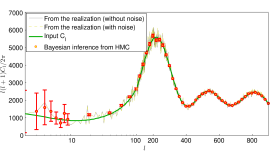
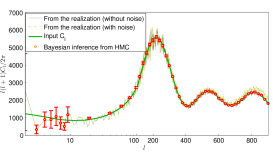
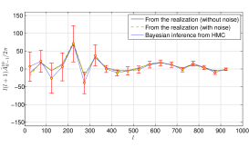
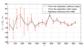
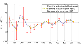
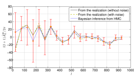
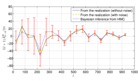
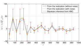
The results are shown in Fig. 1. We test the algorithm at two different noise levels, $\sigma_{n}=10\mu K$ and $\sigma_{n}=20\mu K$. For plots of $C_{l}$ we adopt a hybrid axis which logarithmic up to multipole, $l=100$ and linear beyond. Also, we plot the individual mean values at each multipole, $l\leq 10$, and provide band power average in multipole bin size of $\Delta l=20$ at larger multipoles. The plots show that the algorithm recovers the input power spectrum perfectly up to the high multipoles at both the noise levels. We show the BipoSH coefficients, $\tilde{A}^{10}_{ll-1}$, $\tilde{A}^{20}_{ll}$ and $\tilde{A}^{20}_{ll-2}$ in the 2nd, 3rd and 4th column of Fig. 1. The values of these BipoSH coefficients are consistent with zero within $1$ to $2\sigma$. Though we do not present plots for the other $M\neq 0$ BipoSH coefficients (such as $\tilde{A}^{11}_{ll-1}$,$\tilde{A}^{21}_{ll}$ etc. ), we verify that they are also consistent with zero within $1$ to $2\sigma$.

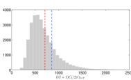
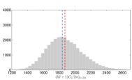
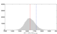
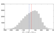
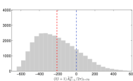
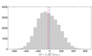
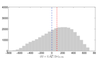
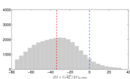
In Fig. 2 we show the marginalised probability distribution of $C_{l}$, $\tilde{A}^{10}_{ll-1}$, $\tilde{A}^{20}_{ll}$ for the multipoles $l=7,\,70,\,700$ respectively for the analysis with $\sigma_{n}=10\mu K$ noise level. In the absence of noise, the inverse of the angular power $C_{l}$ is known to follow the $\Gamma$-distribution that tends to Gaussian at high multipoles. Our analysis shows similar behaviour for the recovered posterior distributions. The theoretical distributions of the $\tilde{A}^{10}_{ll-1}$ and $\tilde{A}^{20}_{ll}$ are not known, although, some exploratory study has been carried out in literature [40].

Figure 3: BipoSH spectra, $\tilde{A}_{ll}^{20}$ and $\tilde{A}_{ll-2}^{20}$, inferred from a non-SI sky map generated by scanning the sky using WMAP-9 beam and scan strategy. The dark grey plot shows the quantities obtained from a direct quadratic estimation from the original sky map and olive dashed curve shows the same quantities after adding noise with the realization. The green plot is the theoretical BipoSH values estimated by averaging the BipoSH samples from 30 simulations. Blue curve with red error-bars show the recovered value of the same from Bayesian inference. The left column corresponds to a noise level of $\sigma_{n}=10\mu K$ and the right column to a noise level of $\sigma_{n}=20\mu K$.ONote that the vertical scales are different in the different plots.

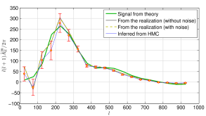
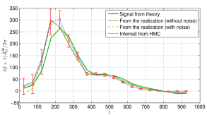
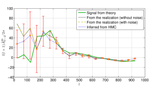
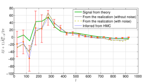
5.2 Beam anisotropy sourced non-SI map

WMAP-7 CMB map showed significant detection of SI violation signal in $\tilde{A}^{20}_{ll}$ and $\tilde{A}^{20}_{ll+2}$ [17]. Later it was revealed that the signal SI violation signals detected were caused due to the mild non-circularity of the beam response of the WMAP experiment coupled to its particular scan pattern [3]. Therefore as a non-SI case study, we take a SI HEALPix map and scan it with a WMAP-like scan strategy using the publicly available (mildly non-circular symmetric) WMAP W1 band beam response maps to generate a simulated time ordered data stream. From the time ordered data we reconstruct the map [2]. This procedure introduces SI violation signatures ($\tilde{A}_{ll}^{20}$ and $\tilde{A}_{ll+2}^{20}$) in the scanned map [3, 4]. We then add white Gaussian noise of amplitude either $10\mu K$ and $20\mu K$ to the maps. These noisy maps are then used to infer the BipoSH spectra.

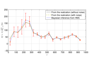
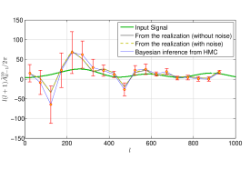
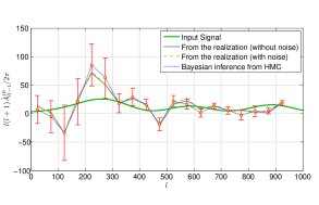
The BipoSH spectra of $\tilde{A}_{ll}^{20}$ and $\tilde{A}_{ll+2}^{20}$ recovered from the analysis are plotted in Fig. 3. The plot shows that the BipoSH spectra is very well recovered up to a very high $l$. Recovery of $\tilde{A}^{20}_{ll}$ is very good at both the noise levels. We note that $\tilde{A}^{20}_{ll-2}$, however, mildly deviates from the input signal at high multipoles, $l>800$.

Figure 4: $\tilde{A}_{ll+1}^{10}$ estimated from a non-SI skymap generated multiplying a SI map with $(.95+0.5T_{d})$, where $T_{d}$ is a dipole modulation oriented along the $\hat{z}$ direction. The light gray and green plot show the $\tilde{A}_{ll+1}^{10}$ quadratic estimations from the original skymap before and after adding noise. Blue curve with red error-bars shows the recovered value of the same from our inference. For this analysis we use $\sigma_{n}=10\mu K$.

5.3 Dipolar modulation non SI map

In the second non-SI case study, we consider a dipole modulated sky map. We generate a SI skymap $T(\gamma)$ using HEALPix and then multiply it with $(.95+0.5T_{d})$ where $T_{d}$ is a dipole modulation oriented along $z$ direction. The map, thus generated, has explicit SI violation signals captured in $\tilde{A}^{10}_{ll-1}$. Then we add instrumental noise at $\sigma_{n}=10\mu K$ to the map. From this map we recover the signal in $\tilde{A}^{10}_{ll-1}$. The results are shown in Fig. 4. It can be seen that the recovery is good at all the multipoles.

5.4 Non-SI inference in the context of a physical model: Doppler boost

Due to the motion of our galaxy with respect to the CMB rest frame the observed CMB signal experiences Doppler boost. Apart from boosting the monopole temperature, the Doppler boost also affects the CMB temperature fluctuations. Its effect on the temperature fluctuations are two fold. Firstly, it produces a modulation effect, that amplifies the temperature along the velocity direction and reduces in the opposite direction. Second effect is the relativistic aberration effect that squashes the anisotropy pattern on one side of the sky and stretches it on the other, effectively mixing the angular scale. As a result a specific form of SI violation is introduced in the CMB maps. Planck 2013 results measured the non-SI signal associated with effect of the Doppler boost [19, 37]. In the final non-SI case study, we generate a non-SI sky map consistent with the signal from the Doppler boost along the $\hat{z}$ direction using CoNIGS [41]. As earlier, we add Gaussian white noise with amplitude $10\mbox{$\mu$K}$ and $20\mu K$ and run our analysis on the noisy maps thus produced to recover the BipoSH spectra. The results of the recovery of the relevant $A^{10}_{ll+1}$ BipoSH spectra is shown in Fig. 5. The figure shows the values of $\tilde{A}_{ll+1}^{10}$ recovered from a particular realization at two different noise levels. For both noise levels, the recovered values match very well with those estimated from the input map. The recovered means are plotted as plotted as band power averages in multipole bins, $\Delta l=50$.

In this particular known cause of SI violation, the non-SI signal in BipoSH is very simply related to the Doppler boost vector, $\vec{\beta}={\vec{v}}/{c}$ related to our peculiar motion with respect to the CMB rest frame.. Hence, as an illustration of non-SI parameter inference readily possible in our methodology, we carry out a Bayesian inference of the boost parameter, $\beta^{1M}$, where $\beta^{1M}=\int\beta Y^{*1M}d\Omega$ is the spherical harmonic decomposition of $\beta=\frac{v}{c}$.

Figure 5: The BipoSH $\tilde{A}_{ll+1}^{10}$ estimated from a SI violation arising from Doppler boost along $\hat{z}$ direction. The non-SI signal map is generated using CoNIGS. The dark green plot is the input signal. Light green and grey plot show the $\tilde{A}_{ll+1}^{10}$ from the original sky map before and after adding noise. Blue curve with red error-bars shows the recovered value of our HMC based inference. Left plot is for $\sigma_{n}=10\mu K$ and the right plot is for $\sigma_{n}=20\mu K$. The recovery of $\tilde{A}_{ll+1}^{10}$ is accurate up to very high $l$.

The posterior of $\beta^{1M}$ can be obtained by directly sampling the $\beta^{1M}$ from the probability distribution $P(S_{lml^{\prime}m^{\prime}},a_{lm}|d_{lm})$ and considering that the only SI violation signal in the map originates from the Doppler boost. Under such assumption $A^{1M}_{ll^{\prime}}=\beta^{1M}H^{M}_{ll^{\prime}}$ and all other BipoSH coefficients are $0$. The equation of motion for $\beta^{1M}$ can be obtained as

$$\dot{p}_{\beta^{1M}}=\frac{\partial\ln P(S_{lml^{\prime}m^{\prime}},a_{lm}|d_{lm})}{\partial\beta^{1M}}=\sum_{l}\frac{\partial A^{1M}_{ll+1}}{\partial\beta^{1M}}\frac{\partial\ln P(S_{lml+1m^{\prime}},a_{lm}|d_{lm})}{\partial A^{1M}_{ll+1}}$$ (5.1)

and

$$\dot{\beta}^{1M}=\frac{p_{{\beta}^{1M}}}{m_{{\beta}^{1M}}}\,.$$ (5.2)

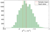
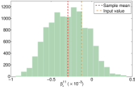
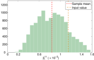
We take the mass parameter $m_{\beta^{1M}}=1$. We can integrate these equations and infer the posterior of $\beta^{1M}$. In Fig. (6) we inferred $\beta^{1M}$ from a SI violated map generated using CoNIGS [41]. The known Doppler boost injected corresponds to $\beta^{10}=-1.87\times 10^{-3}$ and $\beta^{11}=-1.24\times 10^{-4}+1.18\times 10^{-3}i$. We add isotropic Gaussian random noise with $\sigma_{n}=20\mu K$. For our analysis, we remove low multipoles and consider the sum of Eq.(5.1) from $201$ to $1024$ multipoles in the range, because at the low multipoles, signal is small but the errorbars being large, introduces unwarranted higher error in determining beta. Note that the recovery of the Doppler signal is expected to improve as one includes higher multipoles up to $l\sim 2000$ now available from Planck. Here, in this demonstrative example on a simulated map, we restrict to $l_{max}=1000$, and also add a noise much higher than that on current CMB experiments to establish the method in a more adverse situation. The analysis demonstrates that models with small number of parameters can be inferred from high-resolution data.

Figure 6: We calculate the posterior of $\beta^{1M}$ from a realization generated from input $\beta^{10}=-1.87\times 10^{-3}$ and $\beta^{11}=-1.24\times 10^{-4}+1.18\times 10^{-3}i$, by directly sampling the likelihood. From the recovered posterior, we obtain the mean $\beta^{10}=-1.76\times 10^{-3}$ and $\beta^{11}=-2.94\times 10^{-4}+0.84\times 10^{-3}i$ The sample map has an isotropic Gaussian random noise $\sigma_{n}=20\mu K$. We generate 11,000 samples which are distributed in 20 bins in each of the plot. The injected value of $\beta^{1M}$ and the sample mean from our analysis are also marked by vertical lines in the graph.

6 Discussion and Conclusion

We design a general method to infer the underlying covariance structure of a random field measured on a sphere using a completely Bayesian technique. We employ the Bipolar Spherical Harmonic representation of the general covariance matrix underlying random fields on a sphere and outline the method for a fully Bayesian inference of the angular power spectrum and the BipoSH coefficients simultaneously from a single observed map. We use Hamiltonian Monte Carlo for sampling the posterior distributions of the BipoSH parametrization of the covariance.

We demonstrate the method with application to simulated CMB sky maps motivated by the need for Bayesian assessment of the presence of the SI violation signal in observed CMB maps. We consider CMB sky maps that are statistically isotropic (SI), as well as, non-SI case studies that carry signatures of a few known cases of SI violation. We test our method at different noise levels. Our method recovers the angular power spectra $C_{l}$ up to high multipoles, $l$, even in presence of large noise. The recovery of the BipoSH spectra is also at good fidelity at all the multipoles up to $l\sim 1000$. In case of the non-SI Doppler boost CMB maps, we also carry out a direct Bayesian inference of the posterior distribution of the the governing boost paramter, $\vec{\beta}$. The recovery of the Doppler signal is expected to improve as one includes higher multipoles up to $l\sim 2000$ now available from Planck and the appropriate noise level that is much lower than employed here. We expect that an application of our method to recently released exquisite CMB sky maps from Planck will provide reliable assessment of SI violation and serve as a valuable tool to assess the level of evidence for or agains the candidate anomalies. Most assessments of non-SI signals have to assume the angular power spectrum. Hence, it is also important to note that here we jointly infer the angular power spectrum together with BipoSH spectra which makes it specifically sensitive to non-SI phenomena that affect both, a known example of which is non-trivial topology of the Universe [42, 43]. Besides, hunting for cosmic signal of SI violation, the method provides an excellent diagnostic of non-SI residuals originating from the handling of unavoidable observational tasks, such as, removal of foreground emission, noise inhomogeneity and non symmetric beam response functions. The method should be readily extendable beyond scalar fields to CMB polarisation maps that are already available on the ‘full’ sky and also to shear field maps of future weak lensing observations over large fractions of the sky.

The general, principled, approach to a Bayesian inference of the covariance structure in a random field on a sphere presented here has broad potential for application to other many aspects of cosmology and astronomy, as well as, more distant areas of research like geosciences and climate modelling.

References

- [1] A. Hajian and T. Souradeep, Measuring statistical isotropy of the CMB anisotropy, Astrophys.J. 597 (2003) L5–L8, [astro-ph/0308001].
- [2] S. Das and T. Souradeep, Leakage of power from dipole to higher multipoles due to non-symmetric beam shape of the CMB missions, JCAP 1505 (2015), no. 05 012, [arXiv:1307.0001].
- [3] S. Das, S. Mitra, A. Rotti, N. Pant, and T. Souradeep, Statistical isotropy violation in WMAP CMB maps due to non-circular beams, arXiv:1401.7757.
- [4] N. Joshi, S. Das, A. Rotti, S. Mitra, and T. Souradeep, Revealing Non-circular beam effect in WMAP-7 CMB maps with BipoSH measures of Statistical Isotropy, arXiv:1210.7318.
- [5] T. Souradeep and B. Ratra, Window function for noncircular beam CMB anisotropy experiment, Astrophys.J. 560 (2001) 28, [astro-ph/0105270].
- [6] J. R. Bond, D. Pogosian, and T. Souradeep, Computing CMB anisotropy in compact hyperbolic spaces, Class. Quant. Grav. 15 (1998) 2671–2687, [astro-ph/9804041].
- [7] G. Efstathiou, The Statistical significance of the low CMB multipoles, Mon.Not.Roy.Astron.Soc. 346 (2003) L26, [astro-ph/0306431].
- [8] K. M. Gorski, On Determining the spectrum of primordial inhomogeneity from the Cobe DMR sky maps. 1. Method, Astrophys.J. 430 (1994) L85, [astro-ph/9403066].
- [9] S. P. Oh, D. N. Spergel, and G. Hinshaw, An Efficient technique to determine the power spectrum from cosmic microwave background sky maps, Astrophys.J. 510 (1999) 551, [astro-ph/9805339].
- [10] B. D. Wandelt, D. L. Larson, and A. Lakshminarayanan, Global, exact cosmic microwave background data analysis using Gibbs sampling, Phys.Rev. D70 (2004) 083511, [astro-ph/0310080].
- [11] B. D. Wandelt, E. Hivon, and K. M. Gorski, The pseudo- method: cosmic microwave background anisotropy power spectrum statistics for high precision cosmology, Phys Rev D64 (2001) 083003, [astro-ph/0008111].
- [12] E. Hivon, K. M. Górski, C. B. Netterfield, B. P. Crill, S. Prunet, and F. Hansen, Master of the cosmic microwave background anisotropy power spectrum: A fast method for statistical analysis of large and complex cosmic microwave background data sets, The Astrophysical Journal 567 (2002), no. 1 2.
- [13] M. L. Brown, P. G. Castro, and A. N. Taylor, CMB temperature and polarisation pseudo-C(l) estimators and covariances, Mon. Not. Roy. Astron. Soc. 360 (2005) 1262–1280, [astro-ph/0410394].
- [14] J. Taylor, M. Ashdown, and M. Hobson, Fast optimal CMB power spectrum estimation with Hamiltonian sampling, Mon.Not.Roy.Astron.Soc. 389 (2008) 1284, [arXiv:0708.2989].
- [15] A. Hajian, Efficient Cosmological Parameter Estimation with Hamiltonian Monte Carlo, Phys.Rev. D75 (2007) 083525, [astro-ph/0608679].
- [16] S. Duane, A. Kennedy, B. J. Pendleton, and D. Roweth, Hybrid monte carlo, Physics Letters B 195 (1987), no. 2 216 – 222.
- [17] C. L. Bennett, R. S. Hill, G. Hinshaw, D. Larson, K. M. Smith, J. Dunkley, B. Gold, M. Halpern, N. Jarosik, A. Kogut, E. Komatsu, M. Limon, S. S. Meyer, M. R. Nolta, N. Odegard, L. Page, D. N. Spergel, G. S. Tucker, J. L. Weiland, E. Wollack, and E. L. Wright, Seven-year Wilkinson Microwave Anisotropy Probe (WMAP) Observations: Are There Cosmic Microwave Background Anomalies?, Astrophysical Journal, Supplement 192 (Feb., 2011) 17, [arXiv:1001.4758].
- [18] C. L. Bennett, D. Larson, J. L. Weiland, N. Jarosik, G. Hinshaw, N. Odegard, K. M. Smith, R. S. Hill, B. Gold, M. Halpern, E. Komatsu, M. R. Nolta, L. Page, D. N. Spergel, E. Wollack, J. Dunkley, A. Kogut, M. Limon, S. S. Meyer, G. S. Tucker, and E. L. Wright, Nine-year Wilkinson Microwave Anisotropy Probe (WMAP) Observations: Final Maps and Results, Astrophysical Journal, Supplement 208 (Oct., 2013) 20, [arXiv:1212.5225].
- [19] Planck Collaboration, P. A. R. Ade, N. Aghanim, C. Armitage-Caplan, M. Arnaud, M. Ashdown, F. Atrio-Barandela, J. Aumont, C. Baccigalupi, A. J. Banday, and et al., Planck 2013 results. XXIII. Isotropy and statistics of the CMB, Astronomy and Astrophysics 571 (Nov., 2014) A23, [arXiv:1303.5083].
- [20] G. Ellis, Topology and cosmology, General Relativity and Gravitation 2 (1971), no. 1 7–21.
- [21] J. R. Bond, D. Pogosian, and T. Souradeep, CMB anisotropy in compact hyperbolic universes. 1. Computing correlation functions, Phys. Rev. D62 (2000) 043005, [astro-ph/9912124].
- [22] J. R. Bond, D. Pogosian, and T. Souradeep, CMB anisotropy in compact hyperbolic universes. 2. COBE maps and limits, Phys. Rev. D62 (2000) 043006, [astro-ph/9912144].
- [23] L. Ackerman, S. M. Carroll, and M. B. Wise, Imprints of a Primordial Preferred Direction on the Microwave Background, Phys.Rev. D75 (2007) 083502, [astro-ph/0701357].
- [24] A. R. Pullen and M. Kamionkowski, Cosmic Microwave Background Statistics for a Direction-Dependent Primordial Power Spectrum, Phys.Rev. D76 (2007) 103529, [arXiv:0709.1144].
- [25] A. Rotti, M. Aich, and T. Souradeep, WMAP anomaly : Weak lensing in disguise, ArXiv e-prints (Nov., 2011) [arXiv:1111.3357].
- [26] S. Mukherjee, A. De, and T. Souradeep, Statistical isotropy violation of cmb polarization sky due to lorentz boost, Phys. Rev. D 89 (Apr, 2014) 083005.
- [27] C. Armitage and B. D. Wandelt, Deconvolution map-making for cosmic microwave background observations, Phys. Rev. D70 (2004) 123007, [astro-ph/0410092].
- [28] E. Keihänen and M. Reinecke, ArtDeco: a beam-deconvolution code for absolute cosmic microwave background measurements, Astronomy & Astrophysics 548 (Dec., 2012) A110, [arXiv:1208.1399].
- [29] E. Keihänen, K. Kiiveri, V. Lindholm, M. Reinecke, and A.-S. Suur-Uski, The impact of beam deconvolution on noise properties in CMB measurements: Application to Planck LFI, ArXiv e-prints (June, 2015) [arXiv:1506.0855].
- [30] M. Tegmark, The angular power spectrum of the 4 year COBE data, Astrophys.J. 464 (1996) L35, [astro-ph/9601077].
- [31] K. Gorski, A. Banday, C. Bennett, G. Hinshaw, A. Kogut, et al., Power spectrum of primordial inhomogeneity determined from the four year COBE DMR sky maps, Astrophys.J. 464 (1996) L11, [astro-ph/9601063].
- [32] R. M. Neal, MCMC using Hamiltonian dynamics, ArXiv e-prints (June, 2012) [arXiv:1206.1901].
- [33] M. D. Hoffman and A. Gelman, The No-U-Turn Sampler: Adaptively Setting Path Lengths in Hamiltonian Monte Carlo, ArXiv e-prints (Nov., 2011) [arXiv:1111.4246].
- [34] D. A. Varshalovich, Quantum Theory Of Angular Momemtum. World Scientific, 1988.
- [35] E. Forest and R. D. Ruth, Fourth-order symplectic integration, Physica D: Nonlinear Phenomena 43 (1990), no. 1 105 – 117.
- [36] R. K. J. M. K. Jain, R. K. Iyengar, Numerical Methods for Scientific and Engineering Computation. New age international (P) limited, publishers, 2005.
- [37] Planck Collaboration, Planck 2013 results. XXVII. Doppler boosting of the CMB: Eppur si muove, Astronomy and Astrophysics 571 (Nov., 2014) A27, [arXiv:1303.5087].
- [38] Planck Collaboration, P. A. R. Ade et al., Planck 2015 results. XVI. Isotropy and statistics of the CMB, arXiv:1506.0713.
- [39] K. M. Gorski, E. Hivon, and B. D. Wandelt, Analysis issues for large CMB data sets, in MPA/ESO Cosmology Conference: Evolution of Large Scale Structure: From Recombination to Garching Garching, Germany, August 2-7, 1998, 1998. astro-ph/9812350.
- [40] N. Joshi, A. Rotti, and T. Souradeep, Statistics of Bipolar Representation of CMB maps, Phys. Rev. D85 (2012) 043004, [arXiv:1109.0729].
- [41] S. Mukherjee and T. Souradeep, Statistically anisotropic Gaussian simulations of the CMB temperature field, Phys.Rev. D89 (2014), no. 6 063013, [arXiv:1311.5837].
- [42] Planck Collaboration, P. A. R. Ade et al., Planck 2013 results. XXVI. Background geometry and topology of the Universe, Astron. Astrophys. 571 (2014) A26, [arXiv:1303.5086].
- [43] Planck Collaboration, P. A. R. Ade et al., Planck 2015 results. XVIII. Background geometry & topology, arXiv:1502.0159.