On the tensor-to-scalar ratio in large single-field inflation models

Abstract

We show that generically the tensor-to-scalar ratio in large single-field inflation scenarios is bounded to be larger than $\mathcal{O}(10^{-3})$ for the spectral index in the range favored by observations.

I Introduction

In scenarios of inflation, a necessary step to explain various features of the present universe, the number of $e$-foldings ($N_{e}$) is conventionally taken to be around $50$-$60$ depending on the cosmological history after inflation. The lower bound of $N_{e}$ can be pushed down as long as the reheating temperature after inflation is high enough to provide the relevant physics afterwards (e.g., baryogenesis, production of dark matter, a successful Big-Bang nucleosynthesis). However, the upper bound is saturated at about $60$, since the upper bound of the tensor-to-scalar ratio ($r_{T}<0.1$ Ade:2015xua ) coming from the non-observations of the tensor mode perturbations, puts an upper bound on the energy scale of inflation i.e., $V_{*}^{1/4}\lesssim 2\times 10^{16}\mathinner{\mathrm{GeV}}$.

In conventional Einstein gravity, the tensor-to-scalar ratio is simply proportional to the slow-roll parameter associated with the slop of the inflaton potential. For small field inflation in which the excursion scale of the inflaton can be lowered down far below Planck scale, $r_{T}$ can be extermely small. However, in large-field inflation scenarios, this can not be the case since the $e$-foldings are likely to turn out too large unless the potential has an unphysical sudden change. Hence, $r_{T}$ is likely to be lower-bounded in such scenarios.

In this work, we show that the $e$-foldings required to match observations set a lower bound of $r_{T}$ at around $\mathcal{O}(10^{-3})$ in most of realistic models of large single-field inflation. Our result is consistent with a recent work, Ref. Huang:2015xda , although the approach is different.

II Inflation and the number of $e$-foldings for a given scale

In slow-roll inflation scenario with a potential $V$ of a single scalar field (playing the role of inflaton), the slow-roll parameters are defined as

$$\epsilon\equiv\frac{1}{2}\left|\frac{M_{\rm P}V^{\prime}}{V}\right|^{2},\quad\eta\equiv\frac{M_{\rm P}^{2}V^{\prime\prime}}{V},\quad\xi^{2}\equiv\frac{M_{\rm P}^{4}V^{\prime}V^{\prime\prime}}{V^{2}}$$ (1)

where $M_{\rm P}=2.4\times 10^{18}\mathinner{\mathrm{GeV}}$ is the reduced Planck mass, and ‘$\prime$’ represents derivative with respect to the inflaton field. The power spectrum of scalar and tensor mode perturbations are given by

$$P_{\mathcal{R}}=\left(\frac{H}{2\pi}\right)^{2}\frac{1}{2\epsilon M_{\rm P}^{2}},\quad P_{T}=\left(\frac{H}{2\pi}\right)^{2}\frac{8}{M_{\rm P}^{2}}$$ (2)

respectively, giving a tensor-to-scalar ratio

$$r_{T}\equiv\frac{P_{T}}{P_{\mathcal{R}}}=16\epsilon$$ (3)

The spectral indices of these modes are

$$n_{s}=1-6\epsilon+2\eta,\quad n_{T}=-2\epsilon$$ (4)

Note that $n_{T}=-r_{T}/8$, a consistency relation of inflation in Einstein gravity. For inflation to end smoothly, $\epsilon$ should depend on the scale; although $\eta$ can be constant. The spectral running, $\alpha\equiv dn_{s}/d\ln k$, is given by

$$\alpha=16\epsilon\eta-24\epsilon^{2}-2\xi^{2}$$ (5)

The number of $e$-foldings generated until the end of inflation, since a given cosmological scale (denoted with a subscript ‘_∗’) exits the horizon during inflation, is given by

$$N_{e,*}^{\rm th}\equiv\int_{*}^{e}Hdt\simeq-\frac{1}{M_{\rm P}^{2}}\int_{*}^{e}d\phi\frac{V}{V^{\prime}}$$ (6)

with $\phi$ being the inflaton field. For a given model of inflation (i.e., a specific form of potential $V$), the observed $n_{s}$ fixes $\phi_{*}$ and hence $N_{e,*}^{\rm th}$ is also fixed. Meanwhile, in order for inflation to solve the smoothness problem of Big-Bang cosmology, any two points within our Hubble patch had to be in casual contact at some stage before the end of inflation. That requires a minimum amount of $e$-foldings, that we will denote $N_{e,*}^{\rm obs}$. In order for an inflation scenario to work, $N_{e,*}^{\rm th}=N_{e,*}^{\rm obs}$ is required, and this constrains the possible models of inflation. If there were no more entropy production after the reheating following inflation, the $e$-foldings associated with the Planck pivot scale ($k_{*}=0.05{\rm Mpc}^{-1}$) are given by KT

$$N_{e,*}^{\rm obs} = \frac{1}{3}\ln\left[\frac{2\sqrt{6}\pi^{3}}{3}\frac{s_{0}}{k_{*}^{3}}\left(\frac{V_{*}}{V_{e}}\frac{V_{e}^{\frac{1}{4}}}{M_{\rm P}}\right)^{3}\left(\frac{T_{\rm d}}{V_{e}^{\frac{1}{4}}}\right)\right]$$ (7)

$$\simeq 57.87-\frac{1}{3}\ln\left[\left(\frac{V_{e}}{V_{*}}\right)^{3}\left(\frac{10^{16}\mathinner{\mathrm{GeV}}}{V_{e}^{\frac{1}{4}}}\right)^{3}\frac{V_{e}^{\frac{1}{4}}}{T_{\rm d}}\right]$$

where $s_{0}$ is the present entropy density

$$s_{0}=\frac{2\pi^{2}}{45}g_{*s0}T_{0}^{3}$$ (8)

with $g_{*s0}=3.9091$ being the number of relativistic degrees of freedom and $T_{0}=2.726{\rm K}$ the CMB temperature at the present universe. The subscript ‘_e’ in the right-hand side denotes the value at the end of inflation, and $T_{\rm d}$ is the decay temperature of the inflaton. The current upper-bound on the tensor-to-scalar ratio $r_{T}<0.1$ Ade:2015xua implies

$$V_{*}^{1/4}\lesssim 2\times 10^{16}\mathinner{\mathrm{GeV}}$$ (9)

and the reheating temperature is bounded as

$$1\mathinner{\mathrm{MeV}}\lesssim T_{\rm d}\lesssim V_{*}^{1/4}$$ (10)

Then, setting $V_{*}=V_{e}$, one finds

$$N_{e,*}^{\rm obs}\lesssim 58.56$$ (11)

The lower bound of $N_{e,*}^{\rm obs}$ depends on the post-inflation cosmology as well as $V_{*}$ and $T_{\rm d}$. In particular, there can be an $\mathcal{O}(10)$ additional contribution to the $e$-foldings of inflation from, for example, thermal inflation Lyth:1995hj ; Lyth:1995ka . In this case, the required $e$-foldings from primordial inflation are reduced by that amount. In principle, there can be multiple stages of thermal inflation, providing a few tens of $e$-foldings. However, thermal inflation with more than two stages is non-trivial to realize (or not so realistic), and too much extra $e$-foldings may cause some inconsistency with observations of small scale structure (see for example Hong:2015oqa ). In realistic models, we expect extra $e$-foldings of around $20$ or less Jeong:2004hy ; Kim:2008yu ; Choi:2009qd ; Park:2010qd ; Choi:2012ye . Hence, in this letter we take $\Delta N_{e}=15$ as the plausible maximal extra $e$-foldings with $T_{\rm d}=V_{*}^{1/4}$ for simplicity in the case where thermal inflation is considered.

The number of $e$-foldings in Eq. (6) can be separated into contributions from slow-roll and non-slow-roll (or fast-roll) regions, denoted respectively as $\Delta N_{e,\rm sr}$ and $\Delta N_{e,\rm fr}$, i.e.,

$$N_{e,*}^{\rm th}=\Delta N_{e,\rm sr}+\Delta N_{e,\rm fr}$$ (12)

where

$$N_{e,\rm sr}=\int_{*}^{\times}\frac{d\phi/M_{\rm P}}{\sqrt{2\epsilon}},\quad N_{e,\rm fr}=\int_{\times}^{e}\frac{d\phi/M_{\rm P}}{\sqrt{2\epsilon}}$$ (13)

The value of $\phi_{\times}$ for which the slow-roll approximation breaks down depends on the potential and is rather ambiguous. However, we can take $\epsilon_{\times}\equiv\epsilon(\phi_{\times})\sim\mathcal{O}(0.1)$, and in this case

$$N_{e,\rm fr}<\frac{\Delta\phi/M_{\rm P}}{\epsilon_{\times}}\simeq 2.24\left(\frac{0.1}{\epsilon_{\times}}\right)^{1/2}\frac{\Delta\phi}{M_{\rm P}}$$ (14)

where $\Delta\phi\equiv|\phi_{e}-\phi_{\times}|$ with $\phi_{e}$ being the value of the inflaton at the end of inflation. In large-field models, generically, $\Delta\phi\gtrsim M_{\rm P}\sim 1$, being the precise value model dependent. Hence, as a simple conservative constraint, we require

$$\Delta N_{e,\rm sr}<N_{e,*}^{\rm th}-\Delta N_{e}$$ (15)

with $\Delta N_{e}=0,15$ depending on the existence of thermal inflation.

III Classes of potentials

There are numerous different shapes of potentials for slow-roll inflation. However, in the region of field values where the slow-roll approximation is still valid, inflaton potentials generally fall into one of the following forms,

• Chaotic monomial: $V_{\rm ch}=V_{0}x^{p}$

• Inverse-Hilltop: $V_{\rm iht}=V_{0}\left(1-1/x^{p}+\dots\right)$

• Starobinsky-like: $V_{\rm st}=V_{0}\left(1-e^{-x}+\dots\right)$

• Hilltop: $V_{\rm ht}=V_{0}\left(1-x^{p}+\dots\right)$

where $x=\phi/\mu$ with $\mu$ being a scale characterizing the end of inflation, and $p$ is assumed to be positive definite. Note that, even if the potentials listed above are approximated froms, it is clear that they all are significantly changed as $x\to 1$. Hence, unless the potentials have non-trivial complications around the end of inflation, we expect that inflation ends at $x\sim 1$. In the following subsections, we show the approximate forms of slow-roll parameters and $N_{e,*}^{\rm th}$ or $N_{e,\rm sr}$ (depending on its relevance) which are expected to be valid as long as $\epsilon$ and $\eta$ are much smaller than unity in the region where $V\approx V_{0}$. These approximate expressions are useful to get an idea of the parametric dependences of the relevant quantities. The discrepancies one would get when considereing a complete potential are minor and do not change our argument.

III.1 Chaotic monomial

In this case, the slow-roll parameters take the (exact) form

$$\epsilon=\frac{p^{2}}{2x^{2}}\left(\frac{M_{\rm P}}{\mu}\right)^{2},\quad\eta=\frac{p(p-1)}{x^{2}}\left(\frac{M_{\rm P}}{\mu}\right)^{2}$$ (16)

giving $\eta=2(p-1)\epsilon/p$, and from Eq. (4)

$$\epsilon_{*}=\left(\frac{p}{p+2}\right)\frac{1-n_{s}}{2}$$ (17)

which does not depend on $\mu$. The $e$-foldings are

$$N_{e,*}^{\rm th}=\frac{p}{4}\left(\frac{1}{\epsilon_{*}}-1\right)\simeq\frac{p+2}{2(1-n_{s})}$$ (18)

It is clear that, as $p$ becomes larger than 1, $\eta$ becomes larger than zero, and similarly $\epsilon$. Also, only $p\lesssim 4$ is allowed, othewise too much $e$-foldings are expected. As can be seen from Eq. (17), $\epsilon$ can be lowered down by taking a small $p$. However, in large field scenarios in which $x_{*}>1$ with $\mu\geq M_{\rm P}$, we are constrained to have $p\gtrsim\mathcal{O}(10^{-2})$. Hence, $r_{T}$ is lower-bounded at $\mathcal{O}(10^{-3})$.

III.2 Inverse-Hilltop potential

For $V\approx V_{0}$, the slow-roll parameters can be approximated as

$$\epsilon\approx\frac{p^{2}}{2x^{2(p+1)}}\left(\frac{M_{\rm P}}{\mu}\right)^{2},\quad\eta\approx-\frac{p(p+1)}{x^{p+2}}\left(\frac{M_{\rm P}}{\mu}\right)^{2}$$ (19)

From Eq. (19), we find

$$\eta=-\frac{2(p+1)}{p}\left[\frac{2}{p^{2}(M_{\rm P}/\mu)^{2}}\right]^{q-1}\epsilon^{q}$$ (20)

where

$$\frac{1}{2}<q\equiv\frac{p+2}{2(p+1)}<1$$ (21)

Using Eq. (4) with Eq. (20), one can find $\epsilon_{*}$, at least numerically, as a function of $p$ and $n_{s}$ for a given $\mu$. Note that $\eta/\epsilon=-2x^{p}(p+1)/p$ in this potential, which means that for a given $\eta$, as $p$ goes away from a value around one (or $\mu$ is lowered down), $\epsilon$ decreases. The $e$-foldings for slow-roll regime are

$$N_{e,\rm sr}\approx\frac{x_{*}^{p+2}-x_{\times}^{p+2}}{p(p+2)}\left(\frac{\mu}{M_{\rm P}}\right)^{2}\approx\left(\frac{1}{\eta_{\times}}-\frac{1}{\eta_{*}}\right)\left(\frac{p+1}{p+2}\right)$$ (22)

where $\eta_{\times}$ is found from Eq. (20) with $\epsilon_{\times}=0.1$.

We can explore the limiting cases of $p$ leading to small $\epsilon_{*}$. When $p\to 0$, one finds

$$\epsilon_{*}\simeq\frac{p}{4}\left(1-n_{s}\right),\ N_{e,\rm sr}\simeq\frac{1}{1-n_{s}}$$ (23)

Hence, taking a small $p$, one can lower down $\epsilon_{*}$, but $N_{e,\rm sr}\gtrsim 50$ requires $n_{s}\gtrsim 0.98$ which is out of the 2-$\sigma$ region. On the other hand, if $p\to\infty$,

$$\epsilon_{*}^{1/2}\simeq-\frac{\gamma}{6}\left(1-\sqrt{1+\frac{6(1-n_{s})}{\gamma^{2}}}\right),\ N_{e,\rm sr}\simeq\frac{2}{1-n_{s}}$$ (24)

with $\gamma\equiv\sqrt{2}p(M_{\rm P}/\mu)$. It may be natural and tempting to set $\mu$ to be the Planck scale. However, in principle $\mu$ can be much larger than $M_{\rm P}$ although it may need some fine-tuning or non-trivial (or unnatural) realizations.

III.3 Starobinsky-like

In this case, one finds

$$\epsilon\approx\frac{e^{-2x}}{2}\left(\frac{M_{\rm P}}{\mu}\right)^{2},\quad\eta\approx-e^{-x}\left(\frac{M_{\rm P}}{\mu}\right)^{2}$$ (25)

Note that, as $\mu$ is increased, $\epsilon_{*}$ matching observations increases as well. So, we take $\mu=M_{\rm P}$ to see the smallest allowed $\epsilon_{*}$. From Eq. (25), one finds

$$\eta=-\sqrt{2}\epsilon^{1/2}$$ (26)

leading to

$$\epsilon_{*}^{1/2}=-\frac{\sqrt{2}}{6}\left(1-\sqrt{1+3(1-n_{s})}\right)$$ (27)

which is the same as $\epsilon_{*}^{1/2}$ in Eq. (24) with $\mu/M_{\rm P}=p$. The the number of $e$-foldings for slow-roll regime are

$$N_{e,\rm sr}\approx\frac{1}{\eta_{\times}}-\frac{1}{\eta_{*}}$$ (28)

where $\eta_{\times}$ is obtained from Eq. (26) with $\epsilon_{\times}=0.1$.

III.4 Hilltop potential

In this case, for $0<p<1$ inflaton should be located at a particular region in $0<x<1$ as the initial condition, and this is non-trivial to realize. Also, as $p$ increases, the $\epsilon_{*}$ needed to match observation becomes smaller. So, we consider only $p\geq 2$ in order to avoid irrelevant complications. Slow-roll parameters are given as

$$\epsilon\approx\frac{p^{2}x^{2(p-1)}}{2}\left(\frac{M_{\rm P}}{\mu}\right)^{2},\quad\eta\approx-p(p-1)x^{p-2}\left(\frac{M_{\rm P}}{\mu}\right)^{2}$$ (29)

Note that for $p=2$, $\eta$ is a constant depending on $\mu$ exclusively, and

$$\frac{\mu}{M_{\rm P}}=\frac{2}{\sqrt{1-n_{s}-6\epsilon_{*}}}\geq\frac{2}{\sqrt{1-n_{s}}}\sim\mathcal{O}(10)$$ (30)

For $p\neq 1,2$, $\eta$ can be found in terms of $\epsilon$ from Eqs. (20) and (21) with $p\to-p$. The number of $e$-foldings is

$$N_{e,\rm sr}\approx\left\{\begin{array}[]{ll}\frac{1}{2\eta}\ln\left(\frac{\epsilon_{\times}}{\epsilon_{*}}\right)&:\ p=2\\ \left(\frac{1}{\eta_{\times}}-\frac{1}{\eta_{*}}\right)\left(\frac{p-1}{p-2}\right)&:\ p\neq 1,2\end{array}\right.$$ (31)

Similarly to the case of $V_{\rm iht}$, as $\mu$ decreases, $\epsilon_{*}$ decreases, and we consider $\mu/M_{\rm P}\geq 1$ here too. Note that, if $\mu/M_{\rm P}=p$, as $p\to\infty$, $\epsilon_{*}$ collapses to the one in Eq. (27).

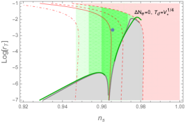
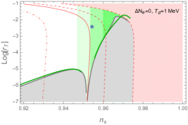
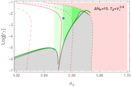
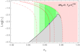
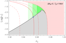
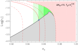
Figure 1: The lower bound of $r_{T}$ (gray line(s)) as a function of $n_{s}$. Green regions are 1, 2, 3-$\sigma$ bands of $n_{s}$ from Planck observations (Planck TT+lowP) Ade:2015lrj . Red lines are obtained by imposing the constraint on the $e$-foldings, Eq. (15). Red dashed lines are for inverse-Hilltop potential with $p=0.1,4$ from right to left. Red dotdashed line is for Hilltop potential with $p=4$. Red solid line is for $p\to\infty$ in both inverse-Hilltop and Hilltop potentials. For each value of $p$, the right-side of the red line is excluded because of too much $e$-foldings. Green line(s) is the bound obtained from the completions of potentials, Eqs. (32), (34) and (33). Blue dot is the prediction of Starobinsky-like potential with $\mu=M_{\rm P}$. Upper: $\mu=M_{\rm P}$. Lower: $\mu=pM_{\rm P}$ for $p\geq 1$, but $\mu=M_{\rm P}$ for $p<1$.

IV The lower bound of $r_{T}$: Numerical results

In order to find a lower bound of $r_{T}$, we used the expressions obtained in the previous section and performed a numerical analysis. Also, for comparsion, we used the following completions of potentials:

$$V_{\rm iht} = V_{0}\left(1-1/2x^{p}\right)^{2}$$ (32)

$$V_{\rm st} = V_{0}\left(1-e^{-x}/2\right)^{2}$$ (33)

$$V_{\rm ht} = V_{0}\left(1-x^{p}/2\right)^{2}$$ (34)

The result is shown in Fig. 1. We found that, if $\mu\sim M_{\rm P}$ (upper panels), when $p\gg 4$ in inverse-Hilltop and Hilltop potentials, it is possible to lower-down $r_{T}$ by many orders of magnitude relative to the current upper bound. However, for $p\leq 4$ which is likely to be the case, in the region of interest the field value is far away from the end point of inflation, and either $r_{T}\gtrsim\mathcal{O}(10^{-3})$ or $n_{s}$ is out of the 3-$\sigma$ bound of observations (in Hilltop). As shown in the lower panels of Fig. 1, if we take $\mu$ larger than $M_{\rm P}$, the case of $p\leq 4$ in Hilltop potential can be within the preferred region of observations, but $r_{T}$ is pushed up to $\mathcal{O}(10^{-3})$. So, we can conlude that, including chaotic monomials and Starobinsky-like potentials, in realistic models (probably) with $p\leq 4$, $r_{T}$ is lower-bounded at about $10^{-3}$ or $n_{s}$ is out-of the 3-$\sigma$ allowed band. Fig. 1 also shows that, if the decay temperature of the inflaton is low or there is an extra contribution to $e$-foldings, the lower-bound of $r_{T}$ is pushed up.

V Conclusions

In this paper, we examined the lower bound of the tensor-to-scalar ratio in large single-field scenarios of inflation. For inflaton field values associated to the relevant cosmological scales, the inflaton potential may be approximated to either chaotic monomial, inverse-Hilltop, Hilltop, or Starobinsky-like potentials in which the leading field-dependent term is $(\phi/\mu)^{\pm p}$ with $0<p\leq 4$ or $e^{-\phi/\mu}$. We showed that, if the dimensionful scale $\mu$ characterizing the end of inflation is Planck scale or larger, which is the case of large single-field scenarios, the tensor-to-scalar ratio is lower-bounded at $\mathcal{O}(10^{-3})$ for the range of the spectral index favored by observations. Therefore, even if it will not be done in the near future, most large single-field inflation models will be probed as experiments reach a $r_{T}$ at the level of $10^{-3}$.

VI Acknowledgements

The authors acknowledge support from the MEC and FEDER (EC) Grants SEV-2014-0398 and FPA2014-54459 and the Generalitat Valenciana under grant PROME- TEOII/2013/017. G.B. acknowledges partial support from the European Union FP7 ITN INVISIBLES (Marie Curie Actions, PITN-GA-2011-289442).

References

• (1) P. A. R. Ade et al. [Planck Collaboration], arXiv:1502.01589 [astro-ph.CO].
• (2) Q. G. Huang, Phys. Rev. D 91, no. 12, 123532 (2015) [arXiv:1503.04513 [astro-ph.CO]].
• (3) E. W. Kolb and M. S. Turner Addison-Wesley Pub. Co. (1994)
• (4) D. H. Lyth and E. D. Stewart, Phys. Rev. Lett.  75, 201 (1995) [hep-ph/9502417].
• (5) D. H. Lyth and E. D. Stewart, Phys. Rev. D 53, 1784 (1996) [hep-ph/9510204].
• (6) S. E. Hong, H. J. Lee, Y. J. Lee, E. D. Stewart and H. Zoe, JCAP 1506, no. 06, 002 (2015)
• (7) D. h. Jeong, K. Kadota, W. I. Park and E. D. Stewart, JHEP 0411, 046 (2004) [hep-ph/0406136].
• (8) S. Kim, W. I. Park and E. D. Stewart, JHEP 0901, 015 (2009) [arXiv:0807.3607 [hep-ph]].
• (9) K. Choi, K. S. Jeong, W. I. Park and C. S. Shin, JCAP 0911, 018 (2009) [arXiv:0908.2154 [hep-ph]].
• (10) W. I. Park, JHEP 1007, 085 (2010) [arXiv:1004.2326 [hep-ph]].
• (11) K. Choi, W. I. Park and C. S. Shin, JCAP 1303, 011 (2013) [arXiv:1211.3755 [hep-ph]].
• (12) P. A. R. Ade et al. [Planck Collaboration], arXiv:1502.02114 [astro-ph.CO].