Measurements of the Ground-State Polarizabilities of Cs, Rb, and K using Atom Interferometry

Abstract

We measured the ground-state static electric-dipole polarizabilities of Cs, Rb, and K atoms using a three-nanograting Mach-Zehnder atom beam interferometer. Our measurements provide benchmark tests for atomic structure calculations and thus test the underlying theory used to interpret atomic parity non-conservation experiments. We measured $\alpha_{\textrm{Cs}}=4\pi\epsilon_{0}\times 59.39(9)\mathrm{\AA}^{3}$, $\alpha_{\textrm{Rb}}=4\pi\epsilon_{0}\times 47.39(8)\mathrm{\AA}^{3}$, and $\alpha_{\textrm{K}}=4\pi\epsilon_{0}\times 42.93(7)\mathrm{\AA}^{3}$. In atomic units, these measurements are $\alpha_{\textrm{Cs}}=401.2(7)$, $\alpha_{\textrm{Rb}}=320.1(6)$, and $\alpha_{\textrm{K}}=290.0(5)$. We report ratios of polarizabilities $\alpha_{\textrm{Cs}}/\alpha_{\textrm{Rb}}=1.2532(10)$, $\alpha_{\textrm{Cs}}/\alpha_{\textrm{K}}=1.3834(9)$, and $\alpha_{\textrm{Rb}}/\alpha_{\textrm{K}}=1.1040(9)$ with smaller fractional uncertainty because the systematic errors for individual measurements are largely correlated. Since Cs atom beams have short de Broglie wavelengths, we developed measurement methods that do not require resolved atom diffraction. Specifically, we used phase choppers to measure atomic beam velocity distributions, and we used electric field gradients to give the atom interference pattern a phase shift that depends on atomic polarizability.

I Introduction

Measurements of static electric-dipole polarizabilities serve as benchmark tests for ab initio calculations of electric-dipole transition matrix elements. These calculations require understanding quantum many-body systems with relativistic corrections, and there are many different methods that attempt to calculate these matrix elements in a reasonable amount of computing time Mitroy et al. (2010). Testing these methods is important because these matrix elements are used to calculate several atomic properties, such as lifetimes, oscillator strengths, line strengths, van der Waals interaction potentials and associated cross sections, Feshbach resonances, and photoassociation rates. Measuring alkali static polarizabilities as a means of testing atomic structure calculations has been of interest to the physics community since Stark’s pioneering measurements in 1934 Scheffers and Stark (1934). Static polarizabilities have been measured using deflection Scheffers and Stark (1934); Chamberlain and Zorn (1963); Hall and Zorn (1974); Ma et al. (2015), an E-H gradient balance Salop et al. (1961); Molof et al. (1974), times-of-flight of an atomic fountain Amini and Gould (2003), and phase shifts in atomic and molecular interferometers Ekstrom et al. (1995); Miffre et al. (2006); Holmgren et al. (2010); Berninger et al. (2007).

We measured the static electric-dipole polarizabilities of K, Rb, and Cs atoms with 0.16% uncertainty using a Mach-Zehnder three-grating atom interferometer Berman (1997); Cronin et al. (2009) with an electric field gradient interaction region. We used the same apparatus for all three elements, so we can also report polarizability ratios with 0.08% uncertainty because the sources of systematic uncertainty are largely correlated between our measurements of different atoms’ polarizabilities.

We compare our measurements to ab initio calculations of atomic polarizabilities and to polarizabilities deduced from studies of atomic lifetimes, Feshbach resonances, and photoassociation specroscopy. We also use our measurements to report the Cs $6p_{1/2}$ and $6p_{3/2}$ state lifetimes, Rb $5p_{1/2}$ and $5p_{3/2}$ state lifetimes, and K $4p_{1/2}$ and $4p_{3/2}$ state lifetimes and the associated principal electric dipole matrix elements, oscillator strengths, and line strengths. Then we use our measurements to report van der Waals $C_{6}$ coefficients, and we combine our measurements with measurements of transition Stark shifts to report some excited state polarizabilities with better than 0.09% uncertainty.

Testing Cs atomic structure calculations by measuring $\alpha_{\textrm{Cs}}$ is valuable for atomic parity non-conservation (PNC) research, which places constraints on beyond-the-standard-model physics. The PNC amplitude $E_{\mathrm{PNC}}$ due to $Z^{0}$-mediated interactions between the Cs valence electron and the neutrons in its nucleus can be written in terms of electric dipole transition matrix elements and the nuclear weak charge parameter $Q_{W}$. Atomic structure calculations are needed to deduce a value of $Q_{W}$ from an $E_{\mathrm{PNC}}$ measurement Blundell et al. (1992); Cho et al. (1997); Derevianko and Porsev (2002); Porsev et al. (2009) to compare to the $Q_{W}$ predicted by the standard model Bouchiat and Bouchiat (1997); Dzuba et al. (2012). Our measurement of $\alpha_{\textrm{Cs}}$ tests the methods used to calculate the relevant matrix elements and provides a benchmark for the $\left.\left\langle 6s_{1/2}\right.\right.\|\hat{D}\|\left.\left.6p_{1/2}\right\rangle\right.$ matrix element, one of the terms in the expression for $E_{\mathrm{PNC}}$.

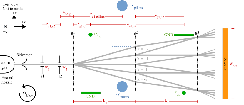
Figure 1: (Color online) Diagram of the Mach-Zehnder atom interferometry apparatus with phase choppers (green) and electrodes that produce an electric field gradient (blue). Dimensions are shown in red and tabulated in Table 1. The supersonic atom beam, shown in gray, is collimated by two slits s1 and s2 with widths $w_{1}$ and $w_{2}$ before entering the first grating. The nanogratings, g1, g2, and g3, are spaced longitudinally such that $L_{1}=L_{2}$, which causes an interference pattern to form at the position of g3. We consider the four separate interferometers in our data analysis, labeled with $k=+2,+1,-1,-2$, that form via 0th, $\pm$1st, and $\pm$2nd order diffraction from g1. The atoms are detected by a platinum Langmuir-Taylor detector Delhuille et al. (2002), indicated in orange. The pair of blue circles represents oppositely-charged cylindrical electrodes (extending perpendicular to the page) that form a virtual ground plane between them. The electric field from these electrodes polarizes the atoms and thereby shifts the interference pattern’s phase. The phase choppers are shown in green; each phase chopper is a charged wire next to a grounded plane. The geometry terms relevant to the pillars and phase choppers are displayed in Fig. 2 and discussed in Section II.1. Due to the rotation of the Earth, the lab has a rotation rate about the vertical axis of $\Omega_{\mathrm{lab},y}=38.88$ $\mu$rad/s that is also relevant to our analysis.

This is the first time that atom interferometry measurements of polarizability have been reported with smaller fractional uncertainty than the pioneering sodium polarizability measurement by Ekstrom et al. in 1995 Ekstrom et al. (1995). This is also, to our knowledge, the first time atom interferometry has been used to measure Cs polarizability. Because it is challenging to resolve Cs atomic diffraction—our nanogratings diffract our Cs atom beams with only 20 $\mu$rad between diffraction orders—we designed an experiment with an electric field gradient instead of a septum electrode, such as was used in Ekstrom et al. (1995); Miffre et al. (2006). We also developed phase choppers Roberts (2002); Roberts et al. (2004); Holmgren et al. (2011); Hromada et al. (2014) to measure our atom beams’ velocity distributions instead of using atom diffraction to study velocity distributions, as was done in Ekstrom et al. (1995); Holmgren et al. (2010). These two innovations enable us to measure polarizabilities of heavy atoms such as Cs without resolving diffraction patterns. Without the need to resolve diffraction, we can use larger collimating slits and a wider detector to obtain data more quickly. These innovations also reduce some systematic errors that are related to beam alignment imperfections.

We improved the accuracy of our measurements compared to our previous work Holmgren et al. (2010) by redesigning the electrodes that apply phase shifts to our interferometer. The new configuration of electrodes, two parallel, oppositely-charged cylindrical pillars, allows us to determine the distance between the atom beam and the virtual ground plane between the pillars with reduced statistical uncertainty. We reduced systematic error by making more accurate measurements of the width of the gap between the pillars, the pillars’ radii, the voltages on the pillars, and the distance between the pillars and the first diffraction grating. Our measurements also required a sophisticated model of the apparatus, which included interference formed by the 0th, $\pm$1st, and $\pm$2nd diffraction orders, the finite thickness and divergence of the beam, and the finite width of the detector Hromada et al. (2014). Because beams of Cs, Rb, and K had different velocity distributions and diffraction angles, we developed a more detailed error analysis in order to understand how those attributes affected the systematic uncertainties in polarizability measurements of different atoms. To support our error analysis, we also developed a method to monitor and adjust the distances between nanogratings in our interferometer.

II Apparatus description and error analysis

Table 1: List of apparatus dimensions described in Fig. 1 and Fig. 2. Dimensions with no quoted uncertainty have uncertainty much less than what would be significant to our analysis. $a_{c1}$ and $a_{c2}$ are the closest distances between the wires and the ground planes for phase choppers 1 and 2, and $a_{\mathrm{pillars}}$ is half the width of the gap between the pillars (the closest distance between the virtual ground plane and either pillar). $L_{1}-L_{2}=0\pm 30$ $\mu$m, and the uncertainty in $L_{1}+L_{2}$ is insignificant.

$z_{\mathrm{s1,s2}}$	860 mm
$z_{\mathrm{g1,pillars}}$	833.5 $\pm$ 0.25 mm
$z_{\mathrm{g1,c1}}$	269.7 mm
$z_{\mathrm{s2,g1}}$	100 mm
$z_{\mathrm{g2,c2}}$	598 mm
$z_{\mathrm{c1,c2}}$	1269.3 $\pm$ 0.25 mm
$L_{1}$	940 mm
$L_{2}$	940 mm
$w_{1}$	30 $\pm$ 6 $\mu$m
$w_{2}$	40 $\pm$ 6 $\mu$m
$w_{\mathrm{det}}$	100 $\pm$ 3 $\mu$m
$a_{\mathrm{pillars}}$	1999.85 $\pm$ 0.5 $\mu$m
$R_{\mathrm{pillars}}$	6350 $\pm$ 0.5 $\mu$m
$a_{c1}$	986 $\pm$ 25 $\mu$m
$R_{c1}$	785.5 $\mu$m
$a_{c2}$	893 $\pm$ 25 $\mu$m
$R_{c2}$	785.5 $\mu$m

A schematic diagram of the three-grating Mach-Zehnder atom beam interferometer we use to make our measurements is shown in Fig. 1. A mixture of He and Ar gas carries Cs, Rb, or K vapor through a 50 $\mu$m nozzle to generate a supersonic atom beam Scoles et al. (1988); Ekstrom (1993). We adjust the carrier gas composition to change the beam’s average velocity: a higher percentage of Ar results in a slower beam. The atom beam passes through two collimating slits and diffracts through three silicon nitride nanogratings, each with period $d_{g}=99.90(0.5)$ nm Savas et al. (1995); Savas (2003). The first two gratings manipulate the atoms’ de Broglie waves to form a 99.90 nm period interference pattern at the position of the third grating. The method of observing interference fringes is described in detail in Kokorowski (2001): we scan the second grating in the $\pm x$ direction and observe the flux admitted through the third grating in order to determine the interference pattern’s contrast and phase. We measure that transmitted atomic flux with a 100 $\mu$m wide platinum wire Langmuir-Taylor detector Delhuille et al. (2002).

In the rest of Section II we describe how we measure the atoms’ velocity distribution and polarizability. We measure $v_{0}$, the atoms’ mean velocity, using phase choppers, which are charged wires parallel with the $y$ axis held parallel to grounded planes, indicated in green in Fig. 1. We measure static polarizability $\alpha$ with a non-uniform electric field created by two oppositely charged cylindrical pillars parallel with the $y$ axis and indicated in blue in Fig. 1. The pillars’ electric field shifts the interference fringe phase by an amount roughly proportional to $\alpha/v_{0}^{2}$. Section II.1 describes how the electric field geoemtry of both the phase choppers and the pillars causes a differential phase shift. Section II.2 describes how we use the phase choppers to measure the velocity distribution, and section II.3 describes how we use the pillars to measure $\alpha$. Section II.4 discusses how we apply our knowledge of the velocity distribution to analyze the polarizability data taken with the pillars.

II.1 Phase shifts with cylindrical electrodes

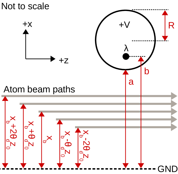
Figure 2: (Color online) Diagram showing the dimensions, shown in red, that describe the static electric fields created by the pillars and by the phase choppers. The circle represents the cross-section of a metal pillar or charged wire with radius $R$ held at voltage $V$. The GND line represents the ground plane, which may by physical (in the case of the choppers) or virtual (in the case of the pillars). $a$ is the closest distance between the pillar edge and the ground plane. The parameter $b$ is the distance between the ground plane and the effective line charge within the pillar. The atom beam center is a distance $x_{b}$ away from the ground plane. The different interferometer arms are separated from their neighbors by multiples of $\theta_{d}z_{0}$, where $\theta_{d}$ is the diffraction angle and $z_{0}$ is the longitudinal distance to grating g1 (in the case of the pillars and chopper c1) or grating g3 (in the case of chopper c2). $a$ and $R$ dimensions for the pillars and phase choppers are given in Table 1.

Both the pillars and the phase choppers are described by the geometry shown in Fig. 2, and create electric fields given by

$$\vec{E}(x,z)=\frac{\lambda}{2\pi\epsilon_{0}}\left[\frac{x-b}{(x-b)^{2}+z^{2}}-\frac{x+b}{(x+b)^{2}+z^{2}}\right]\hat{x}$$

$$+\left[\frac{z}{(x-b)^{2}+z^{2}}-\frac{z}{(x+b)^{2}+z^{2}}\right]\hat{z}$$ (1)

where the effective line charge density

$$\lambda=2\pi\epsilon_{0}V\ln^{-1}\left(\frac{a+R+b}{a+R-b}\right)$$ (2)

exists a distance $b=a\sqrt{1+2R/a}$ away from the ground plane. The parameter $a$ represents the distance between the ground plane and the closest cylinder edge, $R$ represents the pillars’ radius, and the directions $\hat{x}$ and $\hat{z}$ are shown in Fig. 2.

When atoms enter an electric field, their potential energy changes by $U_{\mathrm{Stark}}=-\frac{1}{2}\alpha|\vec{E}|^{2}$. Since $U_{\mathrm{Stark}}\approx-0.1$ $\mu$eV and $E_{\mathrm{kinetic}}\approx$ 1 eV for Cs in our experiment, we can use the WKB approximation along with the Residue Theorem to compute the total phase accumulated by an atom travelling through the field. We can also approximate that atoms travel parallel to the ground plane regardless of the angle at which they diffracted and their incident angle upon grating g1. Even though this approximation may be incorrect by up to $10^{-3}$ rad, such a discrepancy would only cause errors in the accumulated phases by factors of $10^{-6}$, which is insignificant for our experiment. Therefore, we represent the accumulated phase along one path for a component of an atomic de Broglie wave as

$$\Phi(v,x)=\frac{1}{\hbar v}\int_{-\infty}^{\infty}\frac{1}{2}\alpha|\vec{E}|^{2}dz=\frac{\lambda^{2}\alpha}{\pi\epsilon_{0}^{2}\hbar v}\left(\frac{b}{b^{2}-x_{b}^{2}}\right)$$ (3)

where $x_{b}$ is the distance between the atom’s path and the ground plane.

The atoms in our beam form many interferometers, but we only need to consider the four interferometers shown in Fig. 1. Other interferometers are insignificant to our analysis because they have some combination of low contrast and low flux. We label the four interferometers that we do consider with the index $k=+2$, $k=+1$, $k=-1$, and $k=-2$. The differential phase shifts for the four interferometers are

$$\Delta\Phi_{\vec{E},+2}(v,x_{b}) =\Phi(v,x_{b}+2\theta_{d}z_{0})-\Phi(v,x_{b}+\theta_{d}z_{0})$$

$$\Delta\Phi_{\vec{E},+1}(v,x_{b}) =\Phi(v,x_{b}+\theta_{d}z_{0})-\Phi(v,x_{b})$$

$$\Delta\Phi_{\vec{E},-1}(v,x_{b}) =\Phi(v,x_{b})-\Phi(v,x_{b}-\theta_{d}z_{0})$$

$$\Delta\Phi_{\vec{E},-2}(v,x_{b}) =\Phi(v,x_{b}-\theta_{d}z_{0})-\Phi(v,x_{b}-2\theta_{d}z_{0})$$ (4)

In the above equations, $\theta_{d}z_{0}$ is the lateral separation between classical paths in the interferometer, where $\theta_{d}=\lambda_{\mathrm{dB}}/d_{g}$ is the diffraction angle and $z_{0}$ the distance to the first grating (in the case of the pillars and chopper c1) or the third grating (in the case of chopper c2).

II.2 Velocity measurement

The atoms in the beam do not all have the same velocity, so the electric fields do not apply the same phase shifts to each diffracted atom. We observe the average phase and contrast of an ensemble of atoms with velocity distribution $P(v)$. We model $P(v)$ as a Gaussian distribution

$$P(v)=\frac{v_{r}}{v_{0}\sqrt{2\pi}}e^{-\frac{v_{r}^{2}(v-v_{0})^{2}}{2v_{0}^{2}}}$$ (5)

where $v_{0}$ is the mean velocity and the velocity ratio $v_{r}=v_{0}/\sigma_{v}$ is a measure of the distribution’s sharpness. It is worth noting that the velocity distribution for a supersonic atom beam is better described by a $v^{3}$-weighted Gaussian distribution Berman (1997). However, either distribution can be used in our analysis to parametrize the typical high-$v_{0}$, high-$v_{r}$ velocity distributions of our atom beam without changing our polarizability result by more than 0.008%. Since $v_{0}$ is the average velocity in a Gaussian but not in a $v^{3}$-weighted Gaussian, we use Eqn. (5) to simplify our discussion of the error analysis.

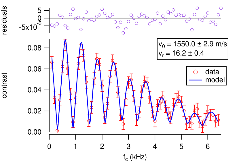
Figure 3: (Color online) An example of a measurement of contrast $C$ vs. phase chopper frequency $f_{c}$ for a Cs beam. We fit a model to these data that has $v_{0}$ and $v_{r}$ as fit parameters in order to measure the velocity distribution.

To measure $v_{0}$ and $v_{r}$, we use phase choppers Holmgren et al. (2011); Hromada et al. (2014). Each phase chopper is a charged wire about 1 mm away from a physical ground plane (see Table 1 for phase chopper dimensions). Chopper c1 is between the first two gratings and chopper c2 is a distance $z_{c1,c2}=1269.3\pm 0.25$ mm downstream of chopper c1, between the last two gratings (see Fig. 1). The voltages on the choppers’ wires and the distances between the beam and the choppers’ ground planes are chosen such that chopper c1 shifts the ensemble’s average phase by $+\pi$ and chopper c2 shifts it by $-\pi$.

When we pulse the choppers on and off at a frequency $f_{c}$, an atom may receive a net phase shift of $\pm\pi$ or $0$ depending on its velocity and the time at which it passed through the first chopper. Holmgren et al. Holmgren et al. (2011) gives an intuitive explanation of how we measure contrast $C$ vs $f_{c}$ to determine $v_{0}$ and $v_{r}$. Fig. 3 shows an example of $C$ vs $f_{c}$ data. Hromada et al. Hromada et al. (2014) later improved upon Holmgren et al.’s model of $C$ vs $f_{c}$ by considering how the thickness and divergence of the beam causes some components of the atoms’ velocity distribution to not be detected. In the present work, we expanded our analysis to include the four interferometers shown in Fig. 1, performed a more in-depth error analysis, and added an additional calibration step to the measurement procedure, as we discuss next.

Hromada et al. described how the thickness and divergence of the beam determines the likelihood for atoms of certain velocities to be detected Hromada et al. (2014). The thickness and divergence is defined by the finite widths of the collimating slits $w_{1}$ and $w_{2}$. The finite width of the detector $w_{\mathrm{det}}$ and the detector’s offset from the beamline in the $x$ direction $\Delta x_{\mathrm{det}}$ also affect the probability of detecting atoms as a function of the atoms’ velocities and initial positions in the apparatus. The phase and contrast we observe with our detector is that of an ensemble of atoms with different velocities, different incident positions on grating g1, and different incident angles on grating g1.

Uncertainties in $w_{1}$, $w_{2}$, $w_{\mathrm{det}}$, and $\Delta x_{\mathrm{det}}$ are more significant for beams that are physically wider. In K beams, which have larger $\theta_{d}$ of $\approx 50$ $\mu$rad and wider velocity distributions ($v_{0}\approx 2100$ m/s, $v_{r}\approx 14$, and therefore $\sigma_{v}\approx 150$ m/s), more of the lower-velocity atoms in the distribution miss the detector. Therefore, uncertainties in the aforementioned quantities have a higher bearing on how we model the average velocity of detected atoms. Ignoring this component of the analysis would cause a systematic increase in measured $v_{0}$ by 0.5% and $v_{r}$ by 10% for a typical K beam.

Modeling the four interferometers shown in Fig. 1, rather than only the $k=\pm 1$ interferometers, also improved our understanding of how likely it is for certain velocities to be detected. For K beams with wide velocity distributions, we would report $v_{0}$ too high by about 0.5% and $v_{r}$ too low by about 5% if we included only the $k=\pm 1$ interferometers. This is because, for such beams, a much higher proportion of atoms in the $k=\pm 2$ interferometers miss the detector than in the $k=\pm 1$ interferometers. Ignoring the $k=\pm 2$ interferometers has a significant effect on the model of the detected $P(v)$ when the detected velocity distributions for the $k=\pm 1$ and $k=\pm 2$ interferometers are significantly different. Conversely, for Cs and Rb beams, we found no significant difference in results between models because most of the atoms in all interferometers were detected regardless of velocity.

Hromada et al. Hromada et al. (2014) also described how inequality between inter-grating distances $L_{1}$ and $L_{2}$ (see Fig. 1) causes systematic errors. When $\Delta L=L_{2}-L_{1}$ is nonzero, the interference fringes formed at the third grating become magnified or demagnified. We summarize this geometric magnification with the separation phase shift:

$$\Delta\Phi_{\mathrm{sep},k}=\frac{2\pi}{d_{g}}\left(\theta_{\mathrm{inc}}+\frac{k}{2}\theta_{d}\right)\Delta L$$ (6)

where $k$ is the interferometer index (see Fig. 1) and $\theta_{\mathrm{inc}}$ is the incident angle on grating g1. To reduce systematic error in our $v_{0}$ and $v_{r}$ measurements, we measure $\Delta L$ and set it equal to zero.

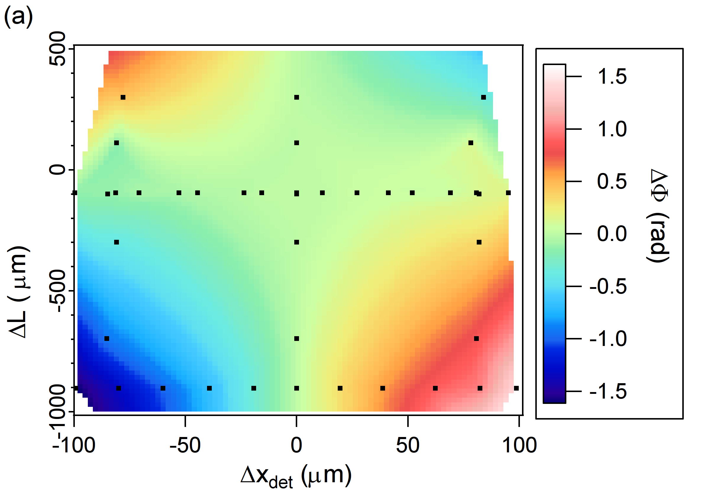
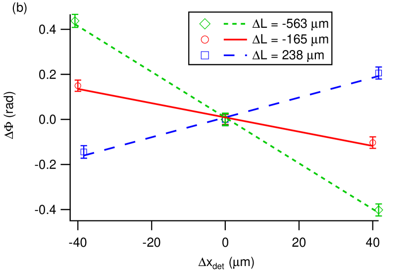
Figure 4: (Color online) Two data plots showing how the phase $\Phi$ of the interference fringes changes linearly as a function of $\Delta x_{\mathrm{det}}$ and $\Delta L$. In plot (a), the black dots represent coordinates at which data was acquired, and the colors represent contours inferred from the data. These figures show how $\Phi$ vs $\Delta x_{\mathrm{det}}$ is a line with slope proportional to $\Delta L$.

Eqn. (6) implies that uncertainty in $\Delta L$ is more significant for beams with larger $\theta_{d}$, such as K beams. Also, because $\Delta\Phi_{\mathrm{sep},k}$ has a component proportional to $\theta_{\mathrm{inc}}$, uncertainty in $\Delta L$ is more significant for more divergent beams. As $|\Delta L|$ increases, uncertainties in $w_{1}$, $w_{2}$, $w_{\mathrm{det}}$, and $\Delta x_{\mathrm{det}}$ become more significant. Accordingly, we developed a method to set $\Delta L=0$ to reduce those uncertainty contributions. Eqn. (6) implies that interferometers on either side of the beamline receive opposite phase shifts. Therefore, by moving the detector in the $\pm x$ direction, we observe linear changes in $\Phi$ as a function of $\Delta x_{\mathrm{det}}$ with slope $\mathrm{d}\Phi/\mathrm{d}x_{\mathrm{det}}$ that is proportional to $\Delta L$. Fig. 4 shows data that demonstrates this effect. We set $\Delta L$ to 0 $\pm$ 30 $\mu$m by finding the $\Delta L$ for which d$\Phi/$d$x_{\mathrm{det}}=0$.

Since we recalibrate $\Delta L$ every day, the 30 $\mu$m uncertainty in $\Delta L$ represents a systematic error for one day’s measurements and a statistical error for many days’ measurements averaged together. That error will contribute toward the statistical uncertainty of $\alpha$ measurements. The same is true for $\Delta x_{\mathrm{det}}=0\pm 30$ $\mu$m, which also fluctuates from day to day as we set up the apparatus.

If the interferometer grating bars are significantly non-vertical, it becomes necessary to consider the phase shift induced by the component of gravitational acceleration in the plane of the interferometer. That phase shift is given by

$$\Delta\Phi_{\mathrm{accel}}=\frac{\pi g\sin({\theta_{g}})(L_{1}+L_{2})^{2}}{2d_{g}v^{2}}$$ (7)

where $\theta_{g}$ is the tilt of the grating bars with respect to vertical Greenberg (2014); Trubko et al. (2015). See Greenberg (2014) for an explanation of how we measured $\theta_{g}$. Our interferometer’s $|\theta_{g}|$ never exceeded 2.3 mrad. If we were to neglect this portion of the analysis, we would report $v_{0}$ incorrectly by up to 0.015% and $v_{r}$ incorrectly by up to 0.25%.

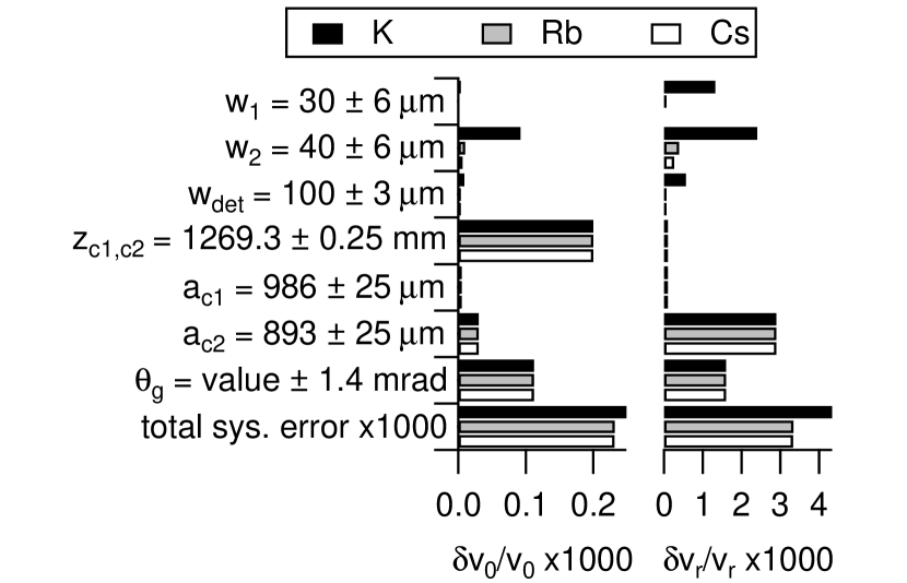
Figure 5: (Color online) Systematic uncertainty budget for measurements of $v_{0}$ and $v_{r}$ for our Cs, Rb, and K beams. The total systematic error in $v_{0}$ and $v_{r}$ in turn contributes toward the total systematic uncertainty in $\alpha$ measurements (shown in Fig. 7). A nominal value for $\theta_{g}$ is not listed because $\theta_{g}$ changed from $-2.37\pm 1.39$ mrad to $1.73\pm 0.59$ mrad toward the end of the experiment.

The uncertainty budget for $v_{0}$ and $v_{r}$ measurements is displayed in Fig. 5. The total statistical uncertainty in measured $v_{0}$ and $v_{r}$ is roughly 10 times larger than the total systematic uncertainty after about 15 minutes of data acquisition with the phase choppers. Because $v_{0}$ and $v_{r}$ drift over time, typically 3% over the course of several hours, we measure the velocity distribution twice every hour.

Gaseous alkali atoms in an atomic beam nozzle have a probability of forming homonuclear dimers that depends on the gas pressure Gordon et al. (1971) and the diameter of the nozzle hole Bergmann et al. (1978). It is important for us to quantify the dimer mole fraction in our beam because the dimers’ spatially averaged (tensor) polarizabilities are approximately 1.75 times the monomer polarizabilities Tarnovsky et al. (1993). In our nozzle, the vapor pressure of alkali atoms is on the order of 1 torr at our typical running temperatures of 160^∘ C for Cs, 220^∘ C for Rb, and 350^∘ C for K. According to data acquired by Gordon et al. (1971) Gordon et al. (1971) and Bergmann et al. (1978) Bergmann et al. (1978), our alkali gas pressures of 1 torr should result in a dimer mole fraction well below 1%. Additionally, Holmgren et al. Holmgren et al. (2010); Holmgren (2013) demonstrated how to place an upper limit on the dimer mole fraction by analyzing resolved diffraction patterns through a single nanograting and looking for peaks associated with dimer diffraction. In this work, we used very similar nozzle temperatures in our experiment as Holmgren et al. did in 2010. For all these reasons, we conclude that the dimer mole fraction in our beam must be less than 1%. Fig. 7 shows how a 4% dimer mole fraction would lead to a significant (0.1%) error in measured polarizability.

II.3 Polarizability measurement

To measure the Cs, Rb, and K polarizability, we use two parallel, oppositely charged, $1/2$-inch-diameter, stainless-steel pillars. The pillars are mounted to a single, rigid support structure so that a 3999.7 $\pm$ 1.0 $\mu$m gap exists between them. A motor moves the support structure in the $\pm x$ direction, and a length gauge monitors the structure’s $x$ position. The length gauge measures displacements of the structure with 30 nm accuracy. We begin a polarizability measurement with the assembly positioned such that the beam passes through the gap between the pillars near one of the edges. We take 25 sec of data with the electric field on and 25 sec with it off. We then move the pillars in nine 400 $\mu$m increments so that the beam approaches the other edge of the gap, taking 50 sec of data at each location. In doing so, we observe the phase shift $\Delta\Phi=\Phi_{\mathrm{pillars,on}}-\Phi_{\mathrm{ref}}$ applied by the pillars as a function of $x_{b}$ (see an example in Fig. 6). We then repeat this sequence, moving the pillars in the opposite direction in order to minimize possible systematic errors associated with travelling in a certain direction. When the electric field is off, we observe the reference phase $\Phi_{\mathrm{ref}}$ and reference contrast $C_{\mathrm{ref}}$ given by

$$C_{\mathrm{ref}}e^{i\Phi_{\mathrm{ref}}}=C_{0}e^{i\Phi_{0}}\frac{1}{2}\sum_{k}\int_{v=0}^{\infty}P(v)e^{i\Delta\Phi_{\mathrm{sag}}(v)}dv$$ (8)

The Sagnac phase, $\Delta\Phi_{\mathrm{sag}}$, is a phase shift caused by the Earth’s rotation and is described in Holmgren et al. (2010); Lenef et al. (1997); Jacquey et al. (2008). $C_{0}$ is the contrast that would be observed in the absence of $\Delta\Phi_{\mathrm{sag}}(v)$, and $\Phi_{0}$ is an arbitrary phase constant. When the field is on, we instead observe

$$C_{\textrm{pillars,on}}e^{i\Phi_{\textrm{pillars,on}}}=$$

$$C_{0}e^{i\Phi_{0}}\frac{1}{2}\sum_{k}\int_{v=0}^{\infty}P(v)e^{i\Delta\Phi_{\vec{E},j}(v,x_{b})+i\Delta\Phi_{\mathrm{sag}}(v)}dv$$ (9)

We fit a model to $\Delta\Phi$ vs $x_{b}$, as shown in Fig. 6. The fit parameters of that model are the polarizability and the pillars position $x_{b0}$ for which the phase shift is zero (i.e. the location of the virtual ground plane).

In our earlier work, we used one pillar next to a grounded plate instead of two pillars forming a virtual ground plane Holmgren et al. (2010). We measured $x_{b}$ by blocking the beam with the pillar. There were significant statistical errors of a few $\mu$m associated with this procedure, and a 1 $\mu$m error would lead to a 0.1% error in polarizability. Our new pillars assembly greatly reduces those statistical errors. Measuring $\Delta\Phi$ vs $x_{b}$ on both sides of the ground plane makes our typical 5 $\mu$m uncertainties in $x_{b0}$ add an insignificant amount of statistical uncertainty to the determined $\alpha$.

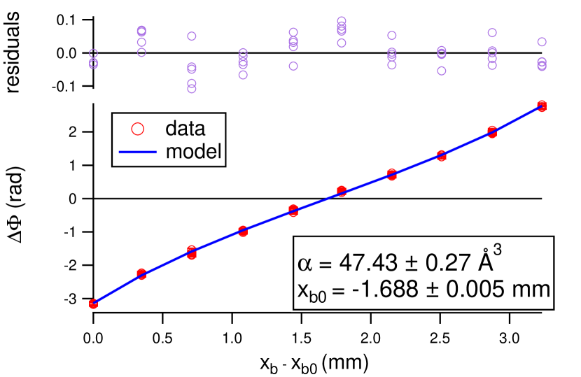
Figure 6: (Color online) An example of a measurement of phase shift vs $x$ position of the pillars for a Rb beam. The two fit parameters used to fit the model to these data are polarizability $\alpha_{\textrm{Rb}}$ and the pillars’ position at which the phase shift is null $x_{b0}$.

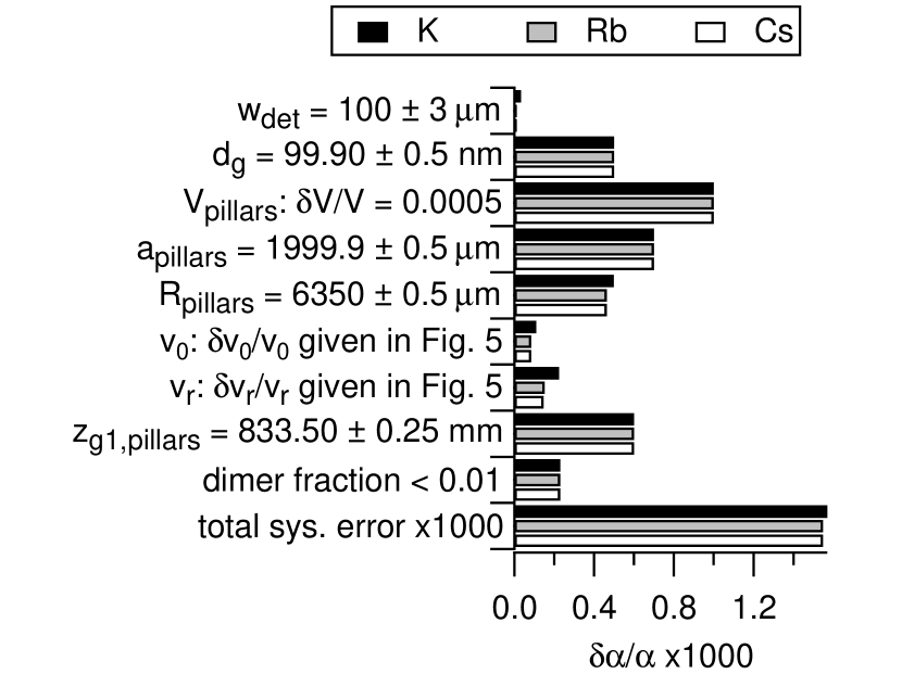
Figure 7: (Color online) Systematic uncertainty budget for polarizability measurements for our Cs, Rb, and K beams. The uncertainties in knowledge of $v_{0}$ and $v_{r}$ are propagated forward from Fig. 5. Values of $V_{\mathrm{pillars}}$ ranged from 5 kV to 7 kV, always with 0.05% uncertainty.

The systematic uncertainty budget for our polarizability measurements is shown in Fig. 7. In the next few paragraphs, we discuss how we measured some of the quantities in the error budget.

We reduced the uncertainty in $V_{\mathrm{pillars}}$ to 0.05% by independently calibrating our voltage supplies. To measure $V_{\mathrm{pillars}}$, which ranged from 5 kV to 7 kV, we used a Fluke 80K-40 high voltage probe. We measured the probe’s voltage divider constant, which itself depended on input voltage, using two Fluke 287 digital multimeters.

We measured $z_{g1,\mathrm{pillars}}$ to 1/4 mm accuracy. We placed rulers in the apparatus, after which three of us would read the rulers both live and from photographs. We repeated this process for many longitudinal positions of the rulers to further reduce statistical error in the measurement. Finally, we compared the rulers we used with other rulers to verify that the ones we used were printed without significant systematic error. The value of $z_{g1,\mathrm{pillars}}$ we use in this analysis is the average of all those measurements.

We measured the width of the gap between the pillars, $2a_{\mathrm{pillars}}$, to 1 $\mu$m accuracy by repeatedly scanning the pillars assembly across the beam and recording the positions at which each pillar blocked half of the atom beam. To verify that $a_{\mathrm{pillars}}$ did not change over time, we repeated this procedure many times throughout the months during which we acquired our data.

Our $\theta_{g}$ was always close enough to zero such that we did not need to consider $\Delta\Phi_{\mathrm{accel}}$ in our polarizability data analysis. We would only need to consider $\Delta\Phi_{\mathrm{accel}}$ if $|\theta_{g}|$ exceeded 23 mrad. We also find that uncertainties in $w_{1}$ and $w_{2}$ each do not correspond to more than 0.004% uncertainty in $\alpha$.

II.4 Determining the velocity distribution during polarizability measurements

Table 2: A typical sequence of measurements during a day of data acquisition. The $+x$ direction is arbitrarily chosen—the important aspect is that we spend an equal amount of time scanning the pillars in each direction so as to minimize possible systematic errors. This sequence of eight measurements is repeated once per hour for anywhere between 8 and 36 hours. We end the data acquisition by repeating the first four measurements.

Type of data acquired	Duration
contrast vs chopping freq.	7m 5s
chopper c1 phase	3m 45s
chopper c2 phase	3m 45s
contrast vs chopping freq.	7m 5s
$\Delta\Phi$ vs pillars position ($+x$ direction)	8m 45s
$\Delta\Phi$ vs pillars position ($-x$ direction)	8m 45s
$\Delta\Phi$ vs pillars position ($+x$ direction)	8m 45s
$\Delta\Phi$ vs pillars position ($-x$ direction)	8m 45s

A typical sequence of measurements is shown in Table 2. We measure the velocity distribution twice between every four scans of the pillars across the beam, and calibrate the phase choppers between each pair of velocity measurements.

We linearly interpolate between $v_{0}$ and $v_{r}$ measurements before and after each pillars scan to estimate those quantities at the time of that scan. Using cubic spline interpolation and Gaussian Process Regression to interpolate between $v_{0}$ and $v_{r}$ measurements changes our reported polarizabilities by no more than 0.001%, which is small compared to our other uncertainties.

III Results and discussion

Table 7 shows our measurement results for the K, Rb, and Cs atomic polarizabilities, $\alpha_{\textrm{K}}$, $\alpha_{\textrm{Rb}}$, and $\alpha_{\textrm{Cs}}$. The tabulated statistical uncertainties are the standard error of the mean for each result. To get this statistical precision, we acquired over 90 hours of data, including 150 data sets similar to Fig. 6 and 60 data sets similar to Fig. 3. The total systematic uncertainty for each measurement is also stated in Table 7, and a breakdown of the systematic uncertainty budget is summarized in Fig. 7. While the statistical uncertainties are typically 0.05% for our measurements of polarizabilities, the systematic uncertainties are three to four times larger, and cause a total uncertainty of typically 0.16% for each measurement.

We report the ratios of polarizabilities $\alpha_{\textrm{Cs}}/\alpha_{\textrm{K}}$, $\alpha_{\textrm{Cs}}/\alpha_{\textrm{Rb}}$, and $\alpha_{\textrm{Rb}}/\alpha_{\textrm{K}}$ in Table 4. These ratios have uncertainties smaller than 0.08% because we used the same apparatus for each direct measurement. For many of the sources of systematic uncertainty summarized in Fig. 7, an error in one of those quantities would scale each direct polarizability measurement by the same amount. These correlated uncertainties, such as electrode geometry or grating pitch, do not contribute significantly to systematic errors in our measured polarizability ratios. However, uncertainties in $w_{1}$, $w_{2}$, $w_{\mathrm{det}}$, and $\Delta L$ affect our $\alpha_{\textrm{K}}$, $\alpha_{\textrm{Rb}}$, and $\alpha_{\textrm{Cs}}$ measurements differently and therefore contribute a small amount to the final systematic uncertainties in the ratios. Even so, the ratios’ systematic errors are much smaller than the statistical uncertainties. We discuss the value of high-precision ratios for testing atomic theories in Section III.1, and we discuss the possibility of using such ratios to improve individual measurements of polarizability in Section IV).

Table 3: Direct measurements of Cs, Rb, and K static, ground-state polarizabilities.

Atom	$\alpha$(stat.)(sys.) ($\mathrm{\AA}^{3}$)
Cs	$59.39(3)(9)$
Rb	$47.39(3)(8)$
K	$42.93(2)(7)$

Table 4: Measured ratios of Cs, Rb, and K static, ground-state polarizabilities. The systematic uncertainties in each ratio, which arise from the fact that the systematic errors in different measurements are not perfectly correlated, are negligible compared to the statistical uncertainties.

Ratio	Value(stat.)	Sys. Err.
$\alpha_{\textrm{Cs}}/\alpha_{\textrm{K}}$	$1.3834(9)$	$3\cdot 10^{-5}$
$\alpha_{\textrm{Cs}}/\alpha_{\textrm{Rb}}$	$1.2532(10)$	$7\cdot 10^{-7}$
$\alpha_{\textrm{Rb}}/\alpha_{\textrm{K}}$	$1.1040(9)$	$2\cdot 10^{-5}$

III.1 Comparisons with other experimental and theoretical polarizabilities

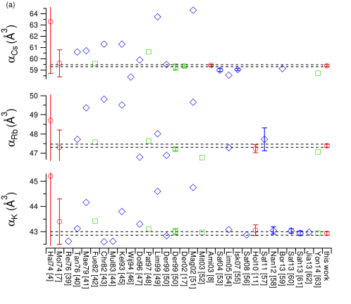
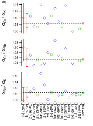
Figure 8: (Color online) Our direct measurements (a) and measured ratios (b) compared with other measurements, ab initio calculations, and semi-empirical calculations Hall and Zorn (1974); Molof et al. (1974); Reinsch and Meyer (1976); Tang (1976); Maeder and Kutzelnigg (1979); Fuentealba (1982); Christiansen and Pitzer (1982); Müller et al. (1984); Kello et al. (1993); van Wijngaarden and Li (1994); Dolg (1996); Patil and Tang (1997); Lim et al. (1999); Derevianko et al. (1999); Magnier and Aubert-Frécon (2002); Derevianko and Porsev (2002); Mitroy and Bromley (2003); Amini and Gould (2003); Safronova and Clark (2004); Lim et al. (2005); Iskrenova-Tchoukova et al. (2007); Safronova and Safronova (2008); Holmgren et al. (2010); Safronova and Safronova (2011); Nandy et al. (2012); Borschevsky et al. (2013); Safronova et al. (2013); Sahoo and Arora (2013); Jiang et al. (2013); Safronova et al. (2013); Yong-Bo et al. (2014). The references are represented on the x-axis by the first three letters of the first author’s last name followed by the year of publication. For the semi-empirical calculations: Reference Fue82 used semi-empirical pseudopotentials Fuentealba (1982), Pat97 used experimentally-determined energy levels Patil and Tang (1997), Der99 used experimentally-determined electric dipole transition matrix elements Derevianko et al. (1999), and Mit03 and Yon14 used semi-empirical core polarization potentials Mitroy and Bromley (2003); Yong-Bo et al. (2014). Values in this plot from 1999 and later are also reported in Table 8 at the end of this paper.

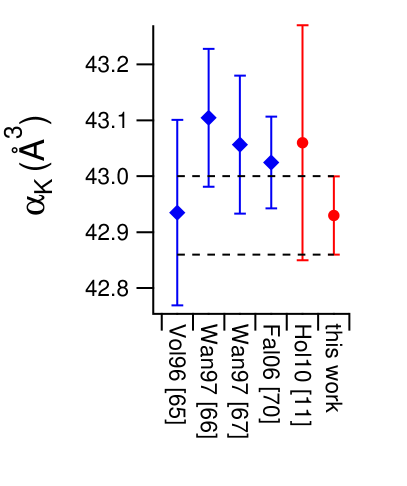
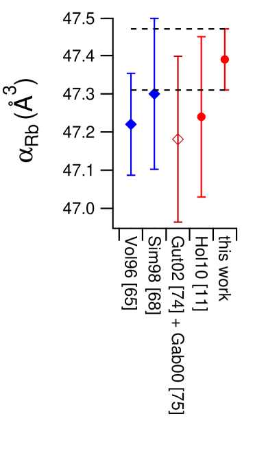
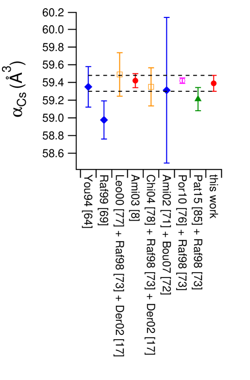
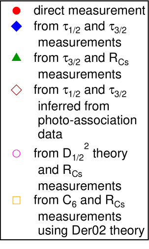
Figure 9: (Color online) Comparisons of our lab’s polarizability measurements (this work as well as Holmgren et al. (2010)) and Amini and Gould’s $\alpha_{\textrm{Cs}}$ measurement Amini and Gould (2003) to polarizabilities derived from measured lifetimes and lifetime ratios, Young et al. (1994); Volz and Schmoranzer (1996); Wang et al. (1997a, b); Simsarian et al. (1998); Rafac et al. (1999); Falke et al. (2006a); Amiot et al. (2002); Bouloufa et al. (2007); Rafac and Tanner (1998), lifetimes inferred from photo-association data Gutterres et al. (2002); Gabbanini et al. (2000), theoretical $D^{2}$ values Porsev et al. (2010), and van der Waals $C_{6}$ measurements Leo et al. (2000); Chin et al. (2004); Derevianko and Porsev (2002). Values in this plot from 1999 and later are also reported in Table 8 at the end of this paper.

Fig. 8 and Table 8 compare our polarizability measurements with ab initio calculations, semi-empirical calculations, and experimental measurements subsequent to and including Molof et al.’s and Hall et al.’s 1974 measurements Molof et al. (1974); Hall and Zorn (1974). First, we will discuss the comparison to previous direct measurements. Our K and Rb polarizability measurements have 3 times smaller uncertainty than our group’s previously published direct measurements of $\alpha_{\textrm{K}}$ and $\alpha_{\textrm{Rb}}$ Holmgren et al. (2010), and 10 times smaller uncertainty than the only other direct measurements of $\alpha_{\textrm{K}}$ and $\alpha_{\textrm{Rb}}$, which were made using the E-H gradient balance technique Molof et al. (1974) and the E gradient deflection technique Hall and Zorn (1974). We emphasize that our new measurements are independent of the results in Holmgren et al. (2010) because although we used the same atom interferometer machine, we used a different material nanograting g1, different electrodes with different geometry, a different atom beam velocity measurement technique, a different atom beam source nozzle, and a detector with a different width. Hence, the fact that our new and more precise measurements are consistent with the measurements in Holmgren et al. (2010); Molof et al. (1974); Hall and Zorn (1974) should be regarded as an independent validation of each of these previous results.

There is one other direct measurement of $\alpha_{\textrm{Cs}}$ with uncertainty similar to (and slightly smaller than) ours. Our direct $\alpha_{\textrm{Cs}}$ measurement is 11 times more precise than the result reported using the E-H balance technique Molof et al. (1974), but 1.1 times less precise than Amini and Gould’s 2003 measurement Amini and Gould (2003) that was made using an atomic fountain apparatus. To our knowledge, Amini and Gould’s work is the only polarizability measurement to date that has been accomplished using an atomic fountain, and it produced a remarkable improvement in precision by a factor of 15 as compared to the only previous direct measurements of $\alpha_{\textrm{Cs}}$ Molof et al. (1974); Hall and Zorn (1974). Furthermore, $\alpha_{\textrm{Cs}}$ measurements can test some of the atomic structure theory that is used to interpret atomic parity non-conservation experiments as a way of constraining physics beyond the standard model Blundell et al. (1992); Cho et al. (1997); Derevianko and Porsev (2002); Porsev et al. (2009). Thus, it is particularly important to validate this $\alpha_{\textrm{Cs}}$ result in Amini and Gould (2003). We find that our $\alpha_{\textrm{Cs}}$ measurement is consistent with Amini and Gould’s. Our result $\alpha_{\textrm{Cs}}=59.39(9)\mathrm{\AA}^{3}$ deviates from their result of $\alpha_{\textrm{Cs}}=59.42(8)\mathrm{\AA}^{3}$ by 0.03 $\mathrm{\AA}^{3}$, which is insignificant. Comparing our atom interferometer result with their fountain result serves as a cross-check for both methods. Both measurements also agree with $\alpha_{\textrm{Cs}}$ values inferred from the atomic structure calculations by Derevianko and Porsev (2002) Derevianko and Porsev (2002) and Derevianko et al. (1999) Derevianko et al. (1999) for PNC analysis.

Most theoretical predictions for $\alpha_{\textrm{K}}$, $\alpha_{\textrm{Rb}}$, and $\alpha_{\textrm{Cs}}$ deviate from each other and from our measurements significantly. Out of 28 sets of theoretical predictions shown in Fig. 8, only ten sets of predictions Derevianko et al. (1999); Derevianko and Porsev (2002); Iskrenova-Tchoukova et al. (2007); Safronova and Safronova (2008, 2011); Nandy et al. (2012); Jiang et al. (2013); Sahoo and Arora (2013); Safronova et al. (2013); Borschevsky et al. (2013) are consistent with our results within 3$\sigma$ (where $\sigma$ is the standard deviation of our measurement). Furthermore, the semi-empirical $\alpha_{\textrm{K}}$, $\alpha_{\textrm{Rb}}$, and $\alpha_{\textrm{Cs}}$ values calculated in 1999 by Derevianko et al. Derevianko et al. (1999) are the only predictions that match all three of our own $\alpha_{\textrm{K}}$, $\alpha_{\textrm{Rb}}$, and $\alpha_{\textrm{Cs}}$ measurements to within 3$\sigma$. These predictions Derevianko et al. (1999) were made using measured lifetimes and energies, and Derevianko and Porsev’s later $\alpha_{\textrm{Cs}}$ prediction Derevianko and Porsev (2002) was made using a measured van der Waals $C_{6}$ coefficient. This is an important point because there are now additional data on lifetimes, van der Waals $C_{6}$ measurements, and line strength ratios that can inform new semi-empirical predictions for polarizabilities that we discuss in Section III.2 and Fig. 9.

Fig. 8 (b) compares our measurements of atomic polarizability ratios to other theoretical, semi-empirical, and experimental reports for these ratios. The values we measured for $\alpha_{\textrm{Cs}}/\alpha_{\textrm{K}}$, $\alpha_{\textrm{Cs}}/\alpha_{\textrm{Rb}}$, and $\alpha_{\textrm{Rb}}/\alpha_{\textrm{K}}$ are consistent with all of the previous experimental measurements of these ratios, given the larger uncertainties associated with previous measurements. Comparing theoretical predictions to our measured polarizability ratios serves as a different way to test the theoretical predictions. Since the fractional uncertainties on our measured ratios are smaller than those of our absolute measurements, our ratios serve as a more precise test for theoretical works that predict $\alpha$ values for multiple alkali atoms.

III.2 Comparisons with polarizabilities derived from other quantities

Static polarizabilities can be related to electric dipole transition matrix elements, state lifetimes, oscillator strengths, and van der Waals coefficients. We will describe those relations and compare our $\alpha$ measurements to $\alpha$ values derived from recent calculations and high-precision measurements of those quantities. Those comparisons are shown in Fig. 9 and Table 8.

Table 5: We use the following residual polarizabilities $\alpha_{r}$ and matrix element ratios $R=D_{3/2}^{2}/D_{1/2}^{2}$. The sources for each quantity are cited next to the values in the table.

Atom	$\alpha_{r}$ ($\mathrm{\AA}^{3}$)	$R$
Cs	2.481(16) Derevianko and Porsev (2002)	1.9809(9)	Rafac and Tanner (1998)
Rb	1.562(89) Safronova et al. (2006)	1.996(4)	Volz and Schmoranzer (1996)
K	0.925(45) Safronova et al. (2006)	2.000(4)	Holmgren et al. (2012)

The polarizability (in volume units) of an atom in state $i$ can be written in terms of Einstein A coefficients $A_{ij}$ as

$$\alpha_{i}=\frac{c^{3}}{2}\sum_{j\neq i}\frac{A_{ij}}{\omega_{ij}^{4}}\frac{g_{j}}{g_{i}}+\alpha_{r}$$ (10)

where $\omega_{ik}$ is the transition frequency between states $i$ and $k$, and $g_{n}=2J_{n}+1$ is the degeneracy factor for state $n$. In our case, state $i$ is the ground state. The residual polarizability $\alpha_{r}$ includes terms not explicitly included in the sum, the polarizability of the core electrons, and a correction accounting for correlations between core and valence electrons as described in several references Derevianko et al. (1999); Derevianko and Porsev (2002); Safronova et al. (2006). We will explicitly sum over the principal transitions from $ns_{1/2}$ to $np_{1/2}$ and $np_{3/2}$, where $n=6$ for Cs, $n=5$ for Rb, and $n=4$ for K, and we will include the other transitions in $\alpha_{r}$. We abbreviate the lifetimes associated with the principal transitions to $\tau_{1/2}$ and $\tau_{3/2}$. In our calculations, we use the transition wavelengths $\omega_{ik}$ from references Gerginov et al. (2005, 2006); Falke et al. (2006b); Johansson (1961) and the $\alpha_{r}$ values indicated in Table 5. Fig. 9 shows polarizabilities calculated using measurements of $\tau_{1/2}$ and $\tau_{3/2}$ Young et al. (1994); Rafac et al. (1999); Bouloufa et al. (2007); Falke et al. (2006a); Volz and Schmoranzer (1996); Simsarian et al. (1998); Wang et al. (1997a). Fig. 9 also shows $\alpha_{\textrm{Cs}}$ calculated from values of $\tau_{1/2,\mathrm{Rb}}$ and $\tau_{3/2,\mathrm{Rb}}$ inferred in 2002 by Gutterres et al. from photo-association data taken in 2000 by Gabbanini et al. Gabbanini et al. (2000); Gutterres et al. (2002).

We can use Patterson et al.’s 2015 measurement of $\tau_{3/2,\mathrm{Cs}}$ Patterson et al. (2015) along with a measurement of the ratio of principal transition matrix elements to report $\alpha_{\textrm{Cs}}$. Rafac and Tanner measured the ratio of Cs electric dipole transition matrix elements Rafac and Tanner (1998)

$$R_{\mathrm{Cs}}=\frac{\left|\left.\left\langle 6s_{1/2}\right.\right.\|\hat{D}\|\left.\left.6p_{3/2}\right\rangle\right.\right|^{2}}{\left|\left.\left\langle 6s_{1/2}\right.\right.\|\hat{D}\|\left.\left.6p_{1/2}\right\rangle\right.\right|^{2}}$$ (11)

which is related to the ratio of lifetimes

$$\frac{\tau_{1/2}}{\tau_{3/2}}=\frac{R_{\mathrm{Cs}}}{2}\left(\frac{\omega_{3/2}}{\omega_{1/2}}\right)^{3}$$ (12)

Table 6: Matrix elements, lifetimes, oscillator strengths, line strengths, and van der Waals $C_{6}$ coefficients calculated from our polarizability measurements. We used $R$ values from Table 5. The matrix elements, line strengths, and $C_{6}$ coefficient are expressed in atomic units, while the lifetimes are expressed in SI units. $\delta_{\alpha}$, $\delta_{R}$, and $\delta_{\alpha_{r}}$ represent the uncertainties in the values due to uncertainty in $\alpha$, $R$, and $\alpha_{r}$, respectively. $\delta_{\mathrm{tot}}$ is the total uncertainty in the value. (-) represents a nonzero uncertainty of less than 0.5.

Quantity	Atom	Value	$\delta_{\alpha}$	$\delta_{R}$	$\delta_{\alpha_{r}}$	$\delta_{\mathrm{tot}}$
$D_{1/2}$	Cs	4.508	(4)	(1)	(1)	(4)
	Rb	4.239	(4)	(3)	(4)	(6)
	K	4.101	(3)	(3)	(2)	(5)
$D_{3/2}$	Cs	6.345	(5)	(-)	(1)	(5)
	Rb	5.989	(5)	(2)	(6)	(8)
	K	5.800	(5)	(2)	(3)	(6)
$\tau_{1/2}$ (ns)	Cs	34.77	(5)	(1)	(1)	(6)
	Rb	27.60	(5)	(4)	(5)	(8)
	K	26.81	(4)	(4)	(3)	(6)
$\tau_{3/2}$ (ns)	Cs	30.37	(5)	(-)	(1)	(5)
	Rb	26.14	(5)	(2)	(5)	(7)
	K	26.45	(4)	(2)	(3)	(6)
$f_{1/2}$	Cs	0.3450	(5)	(1)	(1)	(6)
	Rb	0.3433	(6)	(5)	(7)	(10)
	K	0.3317	(6)	(4)	(4)	(8)
$f_{3/2}$	Cs	0.7174	(11)	(1)	(2)	(12)
	Rb	0.6982	(12)	(5)	(14)	(19)
	K	0.6665	(11)	(4)	(7)	(14)
$S_{1/2}$	Cs	20.32	(3)	(1)	(1)	(3)
	Rb	17.97	(3)	(3)	(3)	(5)
	K	16.82	(3)	(2)	(2)	(4)
$S_{3/2}$	Cs	40.26	(6)	(1)	(1)	(6)
	Rb	35.87	(6)	(3)	(7)	(10)
	K	33.64	(6)	(2)	(4)	(7)
$C_{6}$	Cs	6879	(20)	(-)	(7)	(21)
	Rb	4719	(15)	(-)	(26)	(30)
	K	3884	(13)	(-)	(14)	(19)

Table 7: Excited state polarizabilities $\alpha_{np_{1/2}}$, where $n=6$ for Cs, $n=5$ for Rb, and $n=4$ for K. The values were calculated using our measurements and $\alpha_{np_{1/2}}-\alpha_{ns_{1/2}}$ measurements Hunter et al. (1991); Miller et al. (1994).

Atom	$\alpha_{np_{1/2}}$ ($\mathrm{\AA}^{3}$)
Cs	196.81(9)
Rb	120.33(8)
K	89.92(7)

Table 8: Comparisons of directly measured, semi-empirical, and ab initio polarizabilities from 1999 and later. These values are also plotted in Fig. 8 and Fig. 9. Lines with $\alpha_{r}$ in the Method column were calculated using residual polarizabilities $\alpha_{r}$ in Table 5 Derevianko and Porsev (2002); Safronova et al. (2006). Ratios of polarizabilities $\alpha_{\textrm{Rb}}/\alpha_{\textrm{K}}$ = 1.097(5) from Holmgren et al. (2010) and $\alpha_{\textrm{Cs}}/\alpha_{\textrm{Rb}}$ = 1.2532(10), $\alpha_{\textrm{Cs}}/\alpha_{\textrm{K}}$ = 1.3834(9), $\alpha_{\textrm{Rb}}/\alpha_{\textrm{K}}$ = 1.1040(9)ḟrom this work have been reported with smaller fractional uncertainties than the direct measurements listed in this table. For the ab initio method acronyms: CCSD indicates the coupled-cluster approach with single and double excitations of the wavefunctions. The prefix R stands for “relativistic” and the prefix L stands for “linearized”. The suffix T indicates that the authors used perturbative triple excitations of the wavefunctions. See Mitroy et al. (2010) for explanations of these various theoretical methods.

Reference(s)	Method	$\alpha_{\textrm{Cs}}$ ($\mathrm{\AA}^{3}$)	$\alpha_{\textrm{Rb}}$ ($\mathrm{\AA}^{3}$)	$\alpha_{\textrm{K}}$ ($\mathrm{\AA}^{3}$)
Raf99 Rafac et al. (1999); Derevianko and Porsev (2002)	$\tau_{1/2}$, $\tau_{3/2}$ meas. + $\alpha_{r}$	58.97(22)
Der99 Derevianko et al. (1999)	ab initio, RLCCSD	59.50	46.89	42.84
Der99 Derevianko et al. (1999)	semi-empirical	59.26(28)	47.21(9)	43.00(12)
Leo00 Leo et al. (2000); Rafac and Tanner (1998); Derevianko and Porsev (2002)	$C_{6}$ meas. + $R_{\mathrm{Cs}}$ meas. + thry + $\alpha_{r}$	59.49(25)
Gut02 Gutterres et al. (2002); Gabbanini et al. (2000); Safronova et al. (2006)	$\tau_{1/2}$, $\tau_{3/2}$ from PA data + $\alpha_{r}$		47.18(22)
Der02 Derevianko and Porsev (2002)	semi-empirical	59.35(12)
Mag02 Magnier and Aubert-Frécon (2002)	ab initio	64.31	49.64	44.75
Ami03 Amini and Gould (2003)	direct $\alpha_{\textrm{Cs}}$ meas.	59.42(8)
Mit03 Mitroy and Bromley (2003)	semi-empirical		46.78	42.97
Chi04 Chin et al. (2004); Rafac and Tanner (1998); Derevianko and Porsev (2002)	$C_{6}$ meas. + $R_{\mathrm{Cs}}$ meas. + thry + $\alpha_{r}$	59.35(22)
Saf04 Safronova and Clark (2004)	ab initio	59.00(13)
Lim05 Lim et al. (2005)	ab initio, RCCSDT	58.55	47.29	43.08
Fal06 Falke et al. (2006a); Safronova et al. (2006)	$\tau_{1/2}$, $\tau_{3/2}$ meas. + $\alpha_{r}$			43.02(8)
Bou07 Bouloufa et al. (2007); Derevianko and Porsev (2002)	$\tau_{1/2}$, $\tau_{3/2}$ meas. + $\alpha_{r}$	59.31(82)
Isk07 Iskrenova-Tchoukova et al. (2007)	ab initio, RLCCSDT	59.04(10)
Saf08 Safronova and Safronova (2008)	ab initio, RLCCSDT			42.87
Hol10 Holmgren et al. (2010)	direct $\alpha_{\textrm{Rb}}$ and $\alpha_{\textrm{K}}$ meas.		47.24(44)	43.06(36)
Hol10 Holmgren et al. (2010); Ekstrom et al. (1995)	ratio calibrated with $\alpha_{\text{Na}}$		47.24(21)	43.06(21)
Por10 Porsev et al. (2010); Rafac and Tanner (1998); Derevianko and Porsev (2002)	ab initio$D_{1/2}^{2}$ + $R_{\mathrm{Cs}}$ meas. + $\alpha_{r}$	59.42(3)
Saf11 Safronova and Safronova (2011)	ab initio, RCCSD		47.72(59)
Nan12 Nandy et al. (2012)	ab initio, RCCSDT			43.05(15)
Bor13 Borschevsky et al. (2013)	ab initio, RCCSDT	59.13
Saf13 Safronova et al. (2013)	ab initio, RLCCSDT			43.03(9)
Sah13 Sahoo and Arora (2013)	ab initio, RCCSDT			42.94(9)
Jai13 Jiang et al. (2013)	semi-empirical			42.98
Yon14 Yong-Bo et al. (2014)	semi-empirical	58.72	47.07	42.94
Pat15 Patterson et al. (2015); Rafac and Tanner (1998); Derevianko and Porsev (2002)	$\tau_{3/2}$ meas. + $R_{\mathrm{Cs}}$ meas. + $\alpha_{r}$	59.21(13)
This work	direct meas.	$59.39(9)$	$47.39(8)$	$42.93(7)$

We can also report a polarizability using $R_{\mathrm{Cs}}$ Rafac and Tanner (1998) in conjunction with Porsev et al.’s 2010 calculation of $D_{1/2,\mathrm{Cs}}^{2}=20.334$ (in atomic units) Porsev et al. (2010). We can write $\alpha_{i}$ in terms of the electric dipole transition matrix elements as

$$\alpha_{i}=\frac{e^{2}}{12\pi\epsilon_{0}a_{0}^{4}}\sum_{j\neq i}\frac{\left|\left.\left\langle i\right.\right.\|\hat{D}\|\left.\left.j\right\rangle\right.\right|^{2}}{\hbar\omega_{ij}}+\alpha_{r}$$ (13)

where $a_{0}$ is the Bohr radius. As before, we only explicitly consider the $ns_{1/2}-np_{1/2}$ and $ns_{1/2}-np_{3/2}$ matrix elements, where $ns_{1/2}$ is the ground state. We abbreviate the matrix elements associated with the principal transitions to $D_{1/2}$ and $D_{3/2}$.

In 2002, Derevianko and Porsev demonstrated a method for obtaining values of $D_{1/2,\mathrm{Cs}}^{2}$ and $D_{3/2,\mathrm{Cs}}^{2}$ from Cs van der Waals $C_{6}$ coefficients Derevianko and Porsev (2002) and $R_{\mathrm{Cs}}$ Rafac and Tanner (1998). Fig. 9 includes $\alpha$ values derived using experimental Cs $C_{6}$ measurements in conjunction with that method Leo et al. (2000); Chin et al. (2004).

III.3 Other atomic properties derived from our polarizability measurements

Finally, we use our polarizability measurements to report matrix elements, lifetimes, oscillator strengths, line strengths, and van der Waals $C_{6}$ coefficients. In these calculations, we use residual polarizabilities $\alpha_{r}$ and matrix element ratios $R$ from Table 5. To report matrix elements and lifetimes, we use Eqn. (13) and Eqn. (11). $\alpha_{i}$ is given in terms of oscillator strengths $f_{ij}$ as

$$\alpha_{i}=\frac{e^{2}}{4\pi\epsilon_{0}m}\sum_{j\neq i}\frac{f_{ij}}{w_{ij}^{2}}+\alpha_{r}$$ (14)

where $m$ is the electron mass. $\alpha_{i}$ is also given in terms of line strengths $S_{ji}$ as

$$\alpha_{i}=\frac{1}{6\pi\epsilon_{0}\hbar}\sum_{j\neq i}\frac{S_{ji}}{g_{i}\omega_{ij}}+\alpha_{r}$$ (15)

$C_{6}$ can be expressed in terms of dynamic polarizability as

$$C_{6}=\frac{3}{\pi}\int_{0}^{\infty}\alpha(i\omega)^{2}d\omega$$ (16)

Derevianko et al.’s 2010 work tabulates values of $\alpha(i\omega)$ for Cs, Rb, and K atoms among others Derevianko et al. (2010). To derive $C_{6}$ values from our $\alpha(0)$ measurements, we modify Derevianko et al.’s values of $\alpha(i\omega)$ to get

$$\alpha_{\mathrm{new}}(i\omega)=\tilde{\alpha}(i\omega)-\left[\alpha_{\textrm{this work}}(0)-\tilde{\alpha}(0)\right]\frac{\alpha_{p}(i\omega)}{\alpha_{p}(0)}$$ (17)

where $\tilde{\alpha}(i\omega)$ and $\tilde{\alpha}(0)$ refer to values tabulated by Derevianko et al. In the above equation (17), $\alpha_{p}(i\omega)$ is the contribution to $\alpha(i\omega)$ by the principle transitions. The ratio $\alpha_{p}(i\omega)/\alpha_{p}(0)$ is given by

$$\frac{\alpha_{p}(i\omega)}{\alpha_{p}(0)}=\frac{\frac{1}{\omega_{1/2}^{2}+\omega^{2}}+\frac{R\frac{\omega_{1/2}}{\omega_{3/2}}}{\omega_{3/2}^{2}+\omega^{2}}}{\frac{1}{\omega_{1/2}^{2}}+R\frac{\omega_{1/2}}{\omega^{3}_{3/2}}}$$ (18)

Predictions of the parity-non-conserving amplitude, $E_{\mathrm{PNC}}$, in Cs depends heavily on $D_{1/2}$. We note that our Cs $D_{1/2}$ value is consistent with the theoretical Cs $D_{1/2}$ calculated by Porsev et al. in 2010 for the purpose of interpreting PNC data as a test of the standard model Porsev et al. (2010).

Finally, we use our measurements together with recent measurements of Cs, Rb, and K $\alpha_{np_{1/2}}-\alpha_{ns_{1/2}}$ Hunter et al. (1991); Miller et al. (1994) to report excited state polarizabilities $\alpha_{np_{1/2}}$ with better than 0.08% uncertainty. These results are shown in Table LABEL:tablePolExcited and serve as benchmark tests for calculations of dipole transition matrix elements for $p-d$ transitions.

IV Outlook

We are currently exploring ways to measure the polarizability of Li and metastable He, the polarizabilities of which can be accurately calculated. By measuring $\alpha_{\textrm{Cs}}/\alpha_{\mathrm{He*}}$ or $\alpha_{\textrm{Cs}}/\alpha_{\mathrm{Li}}$, we could report $\alpha_{\textrm{Cs}}$ with precision comparable to that of the ratios reported here for the benefit of PNC research. Such a measurement would also act as a calibration of the measurements presented in this work, because it would be independent of systematic errors that may affect our direct measurements.

We are also exploring electron-impact ionization schemes for atom detection, which would allow us to detect most atoms and molecules. Our Langmuir-Taylor detector only allows us to detect alkali metals and some alkaline-Earth metals Delhuille et al. (2002). Installing an electron-impact ionization detector would allow us to broaden the scope of atom interferometry as a precision measurement tool.

This work is supported by NSF Grant No. 1306308 and a NIST PMG. M.D.G. and R.T. are grateful for NSF GRFP Grant No. DGE-1143953 for support.

References

- Mitroy et al. (2010) J. Mitroy, M. S. Safronova, and C. W. Clark, “Theory and applications of atomic and ionic polarizabilities,” J. Phys. B 44, 202001 (2010).
- Scheffers and Stark (1934) H. Scheffers and J. Stark, “Einfluss des elektrischen Feldes auf Alkaliatome im Atomstrahlversuch,” Phys. Z. 35, 625 (1934).
- Chamberlain and Zorn (1963) G. E. Chamberlain and J. C. Zorn, “Alkali polarizabilities by the atomic beam electrostatic deflection method,” Phys. Rev. 129, 677 (1963).
- Hall and Zorn (1974) W. D. Hall and J. C. Zorn, “Measurement of alkali-metal polarizabilities by deflection of a velocity-selected atomic beam,” Phys. Rev. A 10, 1141 (1974).
- Ma et al. (2015) L. Ma, J. Indergaard, B. Zhang, I. Larkin, R. Moro, and W. A. de Heer, “Measured atomic ground-state polarizabilities of 35 metallic elements,” Phys. Rev. A 91, 010501 (2015).
- Salop et al. (1961) A. Salop, E. Pollack, and B. Bederson, “Measurements of the electric polarizabilities of the alkalis using the E-H gradient balance method,” Phys. Rev. 124, 1431 (1961).
- Molof et al. (1974) R. W. Molof, H. L. Schwartz, T. M. Miller, and B. Bederson, “Measurements of electric dipole polarizabilities of the alkali-metal atoms and the metastable noble-gas atoms,” Phys. Rev. A 10, 1131 (1974).
- Amini and Gould (2003) J. M. Amini and H. Gould, “High precision measurement of the static dipole polarizability of cesium.” Phys. Rev. Lett. 91, 153001 (2003).
- Ekstrom et al. (1995) C. R. Ekstrom, J. Schmiedmayer, M. S. Chapman, T. D. Hammond, and D. E. Pritchard, “Measurement of the electric polarizability of sodium with an atom interferometer,” Phys. Rev. A 51, 3883 (1995).
- Miffre et al. (2006) A. Miffre, M. Jacquey, M. Büchner, G. Trénec, and J. Vigué, “Atom interferometry measurement of the electric polarizability of lithium,” Eur. Phys. J. D 38, 353 (2006).
- Holmgren et al. (2010) W. F. Holmgren, M. C. Revelle, V. P. A. Lonij, and A. D. Cronin, “Absolute and ratio measurements of the polarizability of Na, K, and Rb with an atom interferometer,” Phys. Rev. A 81, 053607 (2010).
- Berninger et al. (2007) M. Berninger, A. Stefanov, S. Deachapunya, and M. Arndt, “Polarizability measurements of a molecule via a near-field matter-wave interferometer,” Phys. Rev. A 76, 013607 (2007).
- Berman (1997) P. Berman, ed., Atom Interferometry (Academic Press, San Diego, 1997).
- Cronin et al. (2009) A. D. Cronin, J. Schmiedmayer, and D. E. Pritchard, “Optics and interferometry with atoms and molecules,” Rev. Mod. Phys. 81, 1051 (2009).
- Blundell et al. (1992) S. A. Blundell, J. Sapirstein, and W. R. Johnson, “High-accuracy calculation of parity nonconservation in cesium and implications for particle physics,” Phys. Rev. D 45, 1602 (1992).
- Cho et al. (1997) D. Cho, C. S. Wood, S. C. Bennett, J. L. Roberts, and C. E. Wieman, “Precision measurement of the ratio of scalar to tensor transition polarizabilities for the cesium 6S-7S transition,” Phys. Rev. A 55, 1007 (1997).
- Derevianko and Porsev (2002) A. Derevianko and S. G. Porsev, “High-precision determination of transition amplitudes of principal transitions in Cs from van der Waals coefficient C6,” Phys. Rev. A 65, 053403 (2002).
- Porsev et al. (2009) S. G. Porsev, K. Beloy, and A. Derevianko, “Precision determination of electroweak coupling from atomic parity violation and implications for particle physics,” Phys. Rev. Lett. 102, 181601 (2009).
- Bouchiat and Bouchiat (1997) M.-A. Bouchiat and C. Bouchiat, “Parity violation in atoms,” Reports Prog. Phys. 60, 1351 (1997).
- Dzuba et al. (2012) V. A. Dzuba, J. C. Berengut, V. V. Flambaum, and B. Roberts, “Revisiting parity nonconservation in cesium,” Phys. Rev. Lett. 109, 203003 (2012).
- Delhuille et al. (2002) R. Delhuille, A. Miffre, E. Lavallette, M. Büchner, C. Rizzo, G. Trénec, J. Vigué, H. J. Loesch, and J. P. Gauyacq, “Optimization of a Langmuir-Taylor detector for lithium,” Rev. Sci. Instrum. 73, 2249 (2002).
- Roberts (2002) T. D. Roberts, Measuring Atomic Properties with an Atom Interferometer, Ph.D. thesis, M.I.T. (2002).
- Roberts et al. (2004) T. D. Roberts, A. D. Cronin, M. V. Tiberg, and D. E. Pritchard, “Dispersion compensation for atom interferometry.” Phys. Rev. Lett. 92, 060405 (2004).
- Holmgren et al. (2011) W. F. Holmgren, I. Hromada, C. E. Klauss, and A. D. Cronin, “Atom beam velocity measurements using phase choppers,” New J. Phys. 13, 115007 (2011).
- Hromada et al. (2014) I. Hromada, R. Trubko, W. F. Holmgren, M. D. Gregoire, and A. D. Cronin, “de Broglie wave-front curvature induced by electric-field gradients and its effect on precision measurements with an atom interferometer,” Phys. Rev. A 89, 033612 (2014).
- Scoles et al. (1988) G. Scoles, D. Bassi, U. Buck, and D. Lainé, eds., Atomic and Molecular Beam Methods (Oxford University Press, New York, Oxford, 1988).
- Ekstrom (1993) C. R. Ekstrom, Experiments with a Separated Beam Atom Interferometer, Ph.D. thesis, M.I.T. (1993).
- Savas et al. (1995) T. A. Savas, S. N. Shah, M. L. Schattenburg, J. M. Carter, and H. I. Smith, “Achromatic interferometric lithography for 100-nm-period gratings and grids,” J. Vac. Sci. Technol. B 13, 2732 (1995).
- Savas (2003) T. A. Savas, Achromatic Interference Lithography, Ph.D. thesis, M.I.T. (2003).
- Kokorowski (2001) D. A. Kokorowski, Measuring decoherence and the matter-wave index of refraction with an improved atom interferometer, Ph.D. thesis, M.I.T. (2001).
- Greenberg (2014) J. Greenberg, An atom interferometer gyroscope, Undergraduate honors thesis, U. of AZ (2014).
- Trubko et al. (2015) R. Trubko, J. Greenberg, M. T. St. Germaine, M. D. Gregoire, W. F. Holmgren, I. Hromada, and A. D. Cronin, “Atom Interferometer Gyroscope with Spin-Dependent Phase Shifts Induced by Light near a Tune-Out Wavelength,” Phys. Rev. Lett. 114, 140404 (2015).
- Gordon et al. (1971) R. J. Gordon, Y. T. Lee, and D. R. Herschbach, “Supersonic molecular beams of alkali dimers,” J. Chem. Phys. 54, 2393 (1971).
- Bergmann et al. (1978) K. Bergmann, U. Hefter, and P. Hering, “Molecular beam diagnostics with internal state selection: velocity distribution and dimer formation in a supersonic Na/Na2 beam,” Chem. Phys. 32, 329 (1978).
- Tarnovsky et al. (1993) V. Tarnovsky, M. Bunimovicz, L. Vuskovic, B. Stumpf, and B. Bederson, “Measurements of the dc electric dipole polarizabilities of the alkali dimer molecules, homonuclear and heteronuclear,” J. Chem. Phys. 98, 3894 (1993).
- Holmgren (2013) W. F. Holmgren, Polarizability and magic-zero wavelength measurements of alkali atoms, Ph.D. thesis, U. of AZ (2013).
- Lenef et al. (1997) A. Lenef, T. D. Hammond, E. T. Smith, M. S. Chapman, R. A. Rubenstein, and D. E. Pritchard, “Rotation Sensing with an Atom Interferometer,” Phys. Rev. Lett. 78, 760 (1997).
- Jacquey et al. (2008) M. Jacquey, A. Miffre, G. Trénec, M. Büchner, J. Vigué, and A. Cronin, “Dispersion compensation in atom interferometry by a Sagnac phase,” Phys. Rev. A 78, 013638 (2008).
- Reinsch and Meyer (1976) E. A. Reinsch and W. Meyer, “Finite perturbation calculation for the static dipole polarizabilities of the atoms Na through Ca,” Phys. Rev. A 14, 915 (1976).
- Tang (1976) K. T. Tang, “Upper and lower bounds of two- and three-body dipole, quadrupole, and octupole van der Waals coefficients for hydrogen, noble gas, and alkali atom interactions,” J. Chem. Phys. 64, 3063 (1976).
- Maeder and Kutzelnigg (1979) F. Maeder and W. Kutzelnigg, “Natural states of interacting systems and their use for the calculation of intermolecular forces,” Chem. Phys. 35, 397 (1979).
- Fuentealba (1982) P. Fuentealba, “On the reliability of semiempirical pseudopotentials: dipole polarisability of the alkali atoms,” J. Phys. B 15, L555 (1982).
- Christiansen and Pitzer (1982) P. A. Christiansen and K. S. Pitzer, “Reliable static electric dipole polarizabilities for heavy elements,” Chem. Phys. Lett. 85, 434 (1982).
- Müller et al. (1984) W. Müller, J. Flesch, and W. Meyer, “Treatment of intershell correlation effects in calculations by use of core polarization potentials. Method and application to alkali and alkaline earth atoms,” J. Chem. Phys. 80, 3297 (1984).
- Kello et al. (1993) V. Kello, A. J. Sadlej, and K. Faegri, “Electron-correlation and relativistic contributions to atomic dipole polarizabilities: Alkali-metal atoms,” Phys. Rev. A 47, 1715 (1993).
- van Wijngaarden and Li (1994) W. A. van Wijngaarden and J. Li, “Polarizabilities of Cesium S, P, D, and F States,” J. Quant. Spectrosc. Radiat. Transf. 52, 555 (1994).
- Dolg (1996) M. Dolg, “Fully relativistic pseudopotentials for alkaline atoms: Dirac–Hartree–Fock and configuration interaction calculations of alkaline monohydrides,” Theor. Chim. Acta 93, 141 (1996).
- Patil and Tang (1997) S. H. Patil and K. T. Tang, “Multipolar polarizabilities and two- and three-body dispersion coefficients for alkali isoelectronic sequences,” J. Chem. Phys. 106, 2298 (1997).
- Lim et al. (1999) I. S. Lim, M. Pernpointner, M. Seth, J. K. Laerdahl, P. Schwerdtfeger, P. Neogrady, and M. Urban, “Relativistic coupled-cluster static dipole polarizabilities of the alkali metals from Li to element 119,” Phys. Rev. A 60, 2822 (1999).
- Derevianko et al. (1999) A. Derevianko, W. R. Johnson, M. S. Safronova, and J. F. Babb, “High-precision calculations of dispersion coefficients, static dipole polarizabilities, and atom-wall interaction constants for alkali-metal atoms,” Phys. Rev. Lett. 82, 3589 (1999).
- Magnier and Aubert-Frécon (2002) S. Magnier and M. Aubert-Frécon, “Static dipolar polarizabilities for various electronic states of alkali atoms,” J. Quant. Spectrosc. Radiat. Transf. 75, 121 (2002).
- Mitroy and Bromley (2003) J. Mitroy and M. W. J. Bromley, “Semiempirical calculation of van der Waals coefficients for alkali-metal and alkaline-earth-metal atoms,” Phys. Rev. A 68, 052714 (2003).
- Safronova and Clark (2004) M. S. Safronova and C. W. Clark, “Inconsistencies between lifetime and polarizability measurements in Cs,” Phys. Rev. A 69, 040501 (2004).
- Lim et al. (2005) I. S. Lim, P. Schwerdtfeger, B. Metz, and H. Stoll, “All-electron and relativistic pseudopotential studies for the group 1 element polarizabilities from K to element 119,” J. Chem. Phys. 122, 104103 (2005).
- Iskrenova-Tchoukova et al. (2007) E. Iskrenova-Tchoukova, M. S. Safronova, and U. I. Safronova, “High-precision study of Cs polarizabilities,” J. Comput. Methods Sci. Eng. 7, 521 (2007).
- Safronova and Safronova (2008) U. I. Safronova and M. S. Safronova, “High-accuracy calculation of energies , lifetimes , hyperfine constants , multipole polarizabilities , and blackbody radiation shift in 39K,” Phys. Rev. A 78, 052504 (2008).
- Safronova and Safronova (2011) M. S. Safronova and U. I. Safronova, “Critically evaluated theoretical energies, lifetimes, hyperfine constants, and multipole polarizabilities in 87Rb,” Phys. Rev. A 83, 052508 (2011).
- Nandy et al. (2012) D. K. Nandy, Y. Singh, B. P. Shah, and B. K. Sahoo, “Transition properties of a potassium atom,” Phys. Rev. A 86, 052517 (2012).
- Borschevsky et al. (2013) A. Borschevsky, V. Pershina, E. Eliav, and U. Kaldor, “ studies of atomic properties and experimental behavior of element 119 and its lighter homologs,” J. Chem. Phys. 138, 124302 (2013).
- Safronova et al. (2013) M. S. Safronova, U. I. Safronova, and C. W. Clark, “Magic wavelengths for optical cooling and trapping of potassium,” Phys. Rev. A 87, 052504 (2013).
- Sahoo and Arora (2013) B. K. Sahoo and B. Arora, “Magic wavelengths for trapping the alkali-metal atoms with circularly polarized light,” Phys. Rev. A 87, 023402 (2013).
- Jiang et al. (2013) J. Jiang, L. Y. Tang, and J. Mitroy, “Tune-out wavelengths for potassium,” Phys. Rev. A 87, 032518 (2013).
- Yong-Bo et al. (2014) T. Yong-Bo, L. Cheng-Bin, and Q. Hao-Xue, “Calculations on polarization properties of alkali metal atoms using Dirac-Fock plus core polarization method,” Chin. Phys. B 23, 063101 (2014).
- Young et al. (1994) L. Young, W. T. Hill, S. J. Sibener, S. D. Price, C. E. Tanner, C. E. Wieman, and S. R. Leone, “Precision lifetime measurements of Cs 6 and 6 levels by single-photon counting,” Phys. Rev. A 50, 2174 (1994).
- Volz and Schmoranzer (1996) U. Volz and H. Schmoranzer, “Precision lifetime measurements on alkali atoms and on helium by beam–gas–laser spectroscopy,” Phys. Scr. T65, 48 (1996).
- Wang et al. (1997a) H. Wang, J. Li, X. T. Wang, C. J. Williams, P. L. Gould, and W. C. Stwalley, “Precise determination of the dipole matrix element and radiative lifetime of the 39K 4p state by photoassociative spectroscopy,” Phys. Rev. A 55, R1569 (1997a).
- Wang et al. (1997b) H. Wang, P. L. Gould, and W. C. Stwalley, “Long-range interaction of the K(4s)+K(4p) asymptote by photoassociative spectroscopy. I. The pure long-range state and the long-range potential constants,” J. Chem. Phys. 106, 7899 (1997b).
- Simsarian et al. (1998) J. E. Simsarian, L. A. Orozco, G. D. Sprouse, and W. Z. Zhao, “Lifetime measurements of the 7 levels of atomic francium,” Phys. Rev. A 57, 2448 (1998).
- Rafac et al. (1999) R. J. Rafac, C. E. Tanner, A. E. Livingston, and H. G. Berry, “Fast-beam laser lifetime measurements of the cesium 6p states,” Phys. Rev. A 60, 3648 (1999).
- Falke et al. (2006a) S. Falke, I. Sherstov, E. Tiemann, and C. Lisdat, “The state of up to the dissociation limit,” J. Chem. Phys. 125, 224303 (2006a).
- Amiot et al. (2002) C. Amiot, O. Dulieu, R. F. Gutterres, and F. Masnou-Seeuws, “Determination of the Cs2 0() potential curve and of Cs 6 atomic radiative lifetimes from photoassociation spectroscopy,” Phys. Rev. A 66, 052506 (2002).
- Bouloufa et al. (2007) N. Bouloufa, A. Crubellier, and O. Dulieu, “Reexamination of the pure long-range state of Cs2: Prediction of missing levels in the photoassociation spectrum,” Phys. Rev. A 75, 052501 (2007).
- Rafac and Tanner (1998) R. J. Rafac and C. E. Tanner, “Measurement of the ratio of the cesium D-line transition strengths,” Phys. Rev. A 58, 1087 (1998).
- Gutterres et al. (2002) R. F. Gutterres, C. Amiot, A. Fioretti, C. Gabbanini, M. Mazzoni, and O. Dulieu, “Determination of the 87Rb 5 state dipole matrix element and radiative lifetime from the photoassociation spectroscopy of the long-range state,” Phys. Rev. A 66, 024502 (2002).
- Gabbanini et al. (2000) C. Gabbanini, A. Fioretti, A. Lucchesini, S. Gozzini, and M. Mazzoni, “Cold rubidium molecules formed in a magneto-optical trap,” Phys. Rev. Lett. 84, 2814 (2000).
- Porsev et al. (2010) S. G. Porsev, K. Beloy, and A. Derevianko, “Precision determination of weak charge of 133Cs from atomic parity violation,” Phys. Rev. D 82, 036008 (2010).
- Leo et al. (2000) P. J. Leo, C. J. Williams, and P. S. Julienne, “Collision Properties of Ultracold 133Cs Atoms,” Phys. Rev. Lett. 85, 2721 (2000).
- Chin et al. (2004) C. Chin, V. Vuletić, A. J. Kerman, S. Chu, E. Tiesinga, P. J. Leo, and C. J. Williams, “Precision feshbach spectroscopy of ultracold Cs2,” Phys. Rev. A 70, 032701 (2004).
- Safronova et al. (2006) M. S. Safronova, B. Arora, and C. W. Clark, “Frequency-dependent polarizabilities of alkali-metal atoms from ultraviolet through infrared spectral regions,” Phys. Rev. A 73, 022505 (2006).
- Holmgren et al. (2012) W. F. Holmgren, R. Trubko, I. Hromada, and A. D. Cronin, “Measurement of a wavelength of light for which the energy shift for an atom vanishes,” Phys. Rev. Lett. 109, 243004 (2012).
- Gerginov et al. (2005) V. Gerginov, C. E. Tanner, S. A. Diddams, A. Bartels, and L. Hollberg, “High-resolution spectroscopy with a femtosecond laser frequency comb.” Opt. Lett. 30, 1734 (2005).
- Gerginov et al. (2006) V. Gerginov, K. Calkins, C. E. Tanner, J. J. McFerran, S. Diddams, A. Bartels, and L. Hollberg, “Optical frequency measurements of 6s p (D1) transitions in 133Cs and their impact on the fine-structure constant,” Phys. Rev. A 73, 032504 (2006).
- Falke et al. (2006b) S. Falke, E. Tiemann, C. Lisdat, H. Schnatz, and G. Grosche, “Transition frequencies of the D lines of 39K, 40K, and 41K measured with a femtosecond laser frequency comb,” Phys. Rev. A 74, 032503 (2006b).
- Johansson (1961) I. Johansson, “Spectra of the Alkali Metals in the Lead-Sulphide Region,” Ark. foer Fys. 20, 135 (1961).
- Patterson et al. (2015) B. M. Patterson, J. F. Sell, T. Ehrenreich, M. A. Gearba, G. M. Brooke, J. Scoville, and R. J. Knize, “Lifetime measurement of the cesium level using ultrafast pump-probe laser pulses,” Phys. Rev. A 91, 012506 (2015).
- Hunter et al. (1991) L. R. Hunter, D. Krause, D. J. Berkeland, and M. G. Boshier, “Precise measurement of the Stark shift of the cesium D1 line,” Phys. Rev. A 44, 6140 (1991).
- Miller et al. (1994) K. E. Miller, D. Krause, and L. R. Hunter, “Precise measurement of the Stark shift of the rubidium and potassium D1 lines,” Phys. Rev. A 49, 5128 (1994).
- Derevianko et al. (2010) A. Derevianko, S. G. Porsev, and J. F. Babb, “Electric dipole polarizabilities at imaginary frequencies for hydrogen, the alkali-metal, alkaline-earth, and noble gas atoms,” At. Data Nucl. Data Tables 96, 323 (2010).