Graphic Realizations of Joint-Degree Matrices

Abstract

In this paper we introduce extensions and modifications of the classical degree sequence graphic realization problem studied by Erdős-Gallai and Havel-Hakimi, as well as of the corresponding connected graphic realization version. We define the joint-degree matrix graphic (resp. connected graphic) realization problem, where in addition to the degree sequence, the exact number of desired edges between vertices of different degree classes is also specified. We give necessary and sufficient conditions, and polynomial time decision and construction algorithms for the graphic and connected graphic realization problems. These problems arise naturally in the current topic of graph modeling for complex networks. From the technical point of view, the joint-degree matrix realization algorithm is straightforward. However, the connected joint-degree matrix realization algorithm involves a novel recursive search of suitable local graph modifications. Also, we outline directions for further work of both theoretical and practical interest. In particular, we give a Markov chain which converges to the uniform distribution over all realizations. We show that the underline state space is connected, and we leave the question of the mixing rate open.

1 Introduction

Let $d_{1}\geq d_{2}\geq\ldots\geq d_{n}$ be a sequence of integers. The classical graphic realization problem asks if there a simple graph on $n$ vertices whose degrees are exactly $d_{1}\geq d_{2}\geq\ldots\geq d_{n}$. Erdős and Gallai showed that the natural necessary conditions for graphic realizability, namely that each subset of the highest $k$ degree vertices can absorb their degrees within their subset and the degrees of the remaining vertices: $\sum_{i=1}^{k}d_{i}\leq k(k\!-\!1)+\sum_{i=k+1}^{n}\min\{k,d_{i}\}$, are also sufficient [14, 5]. The well known Havel-Hakimi algorithm [21, 20] achieves a realization in an efficient greedy way. It repeatedly sorts the vertices according to residual unsatisfied degree, picks any vertex of residual degree $d_{i}$, and connects it to the $d_{i}$ vertices of highest residual degree. The process is repeated until all the degrees are satisfied. If one further wants to construct a connected graphic realization (a requirement which is clearly important in networking), Erdős and Gallai showed that the obvious necessary condition $\sum_{i=1}^{n}d_{i}\geq 2(n\!-\!1)$ (i.e., there is a spanning tree) is also sufficient. In particular, it is easy to see that a non-connected realization can be transformed to a connected realization by a sequence of flips, each flip breaking a cycle inside a connected component, and reducing the number of connected components by one. A “flip” picks two edges $xy$ and $uv$ such that $xu$ and $yv$ are not edges, removes $xy$ and $uv$ from the graph, and adds $xu$ and $yv$ to the graph. It is clear that flips do not change the degrees of the graph.

Now, let $V\!=\![n]$ be a set of vertices. Let ${\mathbb{V}}\!=\!\{V_{1},V_{2},\ldots,V_{k}\}$ be a partition of $V$ denoting subsets of vertices with the same degree and let $d:\mathbb{V}\rightarrow{\mathbb{N}}$ be a function denoting the degree of vertices in class $V_{i}$. Let $D\!=\!(d_{ij})$ be a $k\times k$ matrix denoting the number of edges between $V_{i}$ and $V_{j}$; if $i\!=\!j$ it is the number of edges entirely within $V_{i}$. The joint-degree matrix graphic realization problem is, given $\langle{\mathbb{V}},d,D\rangle$, decide whether there is a simple graph $G$ on $V$, such that, $\forall i$ each vertex in $V_{i}$ has degree $d(V_{i})$, $\forall i\neq j$ there are exactly $d_{ij}$ edges between $V_{i}$ and $V_{j}$, and, $\forall i$, there are exactly $d_{ii}$ edges entirely inside $V_{i}$. The joint-degree matrix connected graphic realization problem is to decide whether a connected graphic realization for $\langle{\mathbb{V}},d,D\rangle$ exists. Furthermore, we want to either construct such a realization, or output a certificate that no such graphic connected realization exists. In this paper we give necessary and sufficient conditions, and polynomial (in $n$) time algorithms for the decision and construction of the joint-degree graphic and connected graphic realization problems.

The practical significance of joint-degree matrix realization problems arises in graph models for several classes of complex networks. For instance, in networking, models for Internet topologies are constantly used to simulate network protocols and predict network evolution. Commonly used topology generators, such as GT-ITM [34, 6] which generates random nearly regular graphs, and power-law based generators [16, 2, 1, 27, 23, 19], generate random graphs. However, the properties of topologies constructed using purely random graph models were challenged, most notably in [3, 24]. Using qualitative arguments and striking images, they argued that power law random graphs construct a dense core of nodes with very high degrees, while nodes of smaller degree are mostly attached to the periphery of the network. On the other hand, highly optimized Internet topologies place low degree but very high bandwidth routers at the center of the network, while high degree nodes are mostly placed in the periphery to split the signal manyways toward the end users. To quantify their argument, [24] used a random graph $G_{\rm R}(V,E_{\rm R})$ under several power law models [4, 11, 7, 30, 12], and a real network topology $G(V,E)$. They found that $\sum_{uv\in E_{\rm R}}{\rm deg}(u){\rm deg}(v)$ is much larger than $\sum_{uv\in E}{\rm deg}(u){\rm deg}(v)$. Independently, [28, 29] made the same observation for several other technological and biological networks.

Going one step further, [26, 25] argued that, a determining metric for a graph of given degrees to resemble a real network topology, is the specific number of links between vertices in different degree classes. Using heuristics that presumably approximate the target number of edges between degree classes, [25] constructed graphs strikingly similar to real network topologies. The joint-degree matrix graphic and connected graphic realization problems studied in Sections 2 and 3 formalize the approach of [26, 25]. In general, one would want to construct a uniformly random realization of $\langle{\mathbb{V}},d,D\rangle$. We state this as an open problem in Section 4. However, for practical purposes, the heuristics of [26, 25] achieved very satisfactory results using randomness in a configuration model adjusted to the $\langle{\mathbb{V}},d,D\rangle$ problem. On the other hand, there are no theoretical results concerning the properties of this model. In the same sense, our joint degree matrix realization algorithm in Section 2, also allows substantial randomness in the choice of the edge to be added in each of its greedy steps.

In Section 2 we address the joint-degree matrix graphic realizability problem. We show that the natural necessary conditions are also sufficient, and can be checked efficiently. We also obtain a second polynomial time construction algorithm, which is a key for the algorithm in Section 3. This Balanced Degree Algorithm constructs the graph by increasing the number of edges, without increasing the number of connected components. In Section 3 we address the joint-degree matrix connected graphic realizability problem. By sharp contrast to the degree sequence connected realization, here the necessary and sufficient conditions are fairly complex, and of exponential size. However, using a recursive algorithm that searches for suitable local graph modifications to construct a connected graph, we manage to either construct such a graph in polynomial time, or identify at least one necessary condition that fails to hold. In Section 5 we discuss structural differences between degree sequence and joint-degree matrix problems. In particular, the former are known to be related to matchings, while no corresponding fact is known for the latter. Finally, in Section 5, we propose a natural Markov chain for sampling from $\langle{\mathbb{V}},d,D\rangle$, and we show that it is ergodic.

Recent related work. Independently, [32, 10, 18] give polynomial time algorithms for constructing a graph in $\langle{\mathbb{V}},d,D\rangle$. Moreover, in [32] an alternative proof is proposed for the fact that the Markov chain we define in Section 5 is ergodic. This proof however was flawed, as noted in [10], where an alternative proof is given as well. With respect to the mixing time of this Markov chain, [32] performed experiments based on the autocorrelation of each edge; these experiments suggest that the Markov chain mixes quickly. In a more recent work, [15] shows fast mixing for a related Markov chain over the subset of $\langle{\mathbb{V}},d,D\rangle$ that contains the balanced realizations, i.e. realizations where for each $i,j$ the edges connecting $V_{i}$ to $V_{j}$ are as uniformly distributed on $V_{i}$ as possible. (Notice that this is not what we call a balanced graph, e.g. in Lemma 2 or in Section 3.)

2 Joint-Degree Matrix Graphic Realization

Let $V\!=\![n]$ be a set of vertices and ${\mathbb{V}}\!=\!\{V_{1},V_{2},\ldots,V_{k}\}$ be a partition of $V$ denoting subsets of vertices with the same degree. Let $d:\mathbb{V}\rightarrow{\mathbb{N}}$ be a function denoting the degrees of vertices in class $V_{i}$ and $D\!=\!(d_{ij})$ be a $k\times k$ matrix denoting the number of edges between $V_{i}$ and $V_{j}$; if $i\!=\!j$ it is the number of edges entirely within $V_{i}$. The joint-degree matrix graphic realization problem is, given $\langle{\mathbb{V}},d,D\rangle$, decide whether there is a simple graph $G$ on $V$, such that, $\forall i$ each vertex in $V_{i}$ has degree $d(V_{i})$, $\forall i\neq j$ there are exactly $d_{ij}$ edges between $V_{i}$ and $V_{j}$, and $\forall i$, there are exactly $d_{ii}$ edges entirely inside $V_{i}$. We use the notation $\langle{\mathbb{V}},d,D\rangle$ to also denote the set of all such graphs.

We will prove that the following natural necessary conditions for the instance $\langle{\mathbb{V}},d,D\rangle$ to have a graphic realization are also sufficient:
(i) Degree feasibility: $2d_{ii}\!+\!\sum_{j\in[k],j\neq i}d_{ij}=|V_{i}|\cdot d(V_{i})$, for $1\leq i\leq k$.
(ii) Matrix feasibility: The matrix $D$ is symmetric with nonnegative integral entries, and $d_{ij}\leq|V_{i}|\cdot|V_{j}|$, for $1\leq i<j\leq k$, while $d_{ii}\leq|V_{i}|\cdot(|V_{i}|\!-\!1)/2$, for $1\leq i\leq k$.

There is a straightforward algorithm for constructing a graph $G\in\langle{\mathbb{V}},d,D\rangle$. First, the algorithm constructs a graph $G^{\prime}$ that has the “right” number of edges between any $V_{i}$, $V_{j}$ (or within a $V_{i}$). Then, the degrees within each $V_{i}$ are taken care of, resulting in a graph $G\in\langle{\mathbb{V}},d,D\rangle$.

The algorithm proceeds as follows:
Start with an empty graph $G$ on $V$
For each $i$
     choose arbitrarily $d_{ii}$ edges between vertices of $V_{i}$, and add them to $G$
For each $i,j$
     choose arbitrarily $d_{ij}$ edges between vertices of $V_{i}$ and $V_{j}$, and add them to $G$
For each $i$
     While not all degrees in $V_{i}$ are equal
         Choose $u,v\in V_{i}$ such that ${\rm deg}(u)<d(V_{i})$ and ${\rm deg}(v)>d(V_{i})$
         Find $\min\{|{\rm deg}(u)-d(V_{i})|,|{\rm deg}(v)-d(V_{i})|\}$ neighbors of $v$ that are not neighbors of $u$
         Disconnect them from $v$ and connect them to $u$
Output $G$

To see that the algorithm works, first notice that if $d_{ij}\leq|V_{i}|\cdot|V_{j}|$, for $1\leq i<j\leq k$, and $d_{ii}\leq|V_{i}|\cdot(|V_{i}|\!-\!1)/2$, for $1\leq i\leq k$ the edge-adding part of the algorithm works. This results in a graph $G$ that satisfies the $d_{ij}$ requirements, but not necessarily the degree requirements.

Now, assume that there exist some $i$ such that not all the degrees in $V_{i}$ are equal to $d(V_{i})$. If $2d_{ii}\!+\!\sum_{j\in[k],j\neq i}d_{ij}=|V_{i}|\cdot d(V_{i})$, this means that there exist $u,v\in V_{i}$ such that ${\rm deg}(u)<d(V_{i})$ and ${\rm deg}(v)>d(V_{i})$. Also, there are $|{\rm deg}(u)-{\rm deg}(v)|$ neighbors of $v$ that are non-neighbors of $u$, and $|{\rm deg}(u)-{\rm deg}(v)|>\min\{|{\rm deg}(u)-d(V_{i})|,|{\rm deg}(v)-d(V_{i})|\}$. Also, notice that each iteration in the “while” loop reduces the number of “wrong degrees” by at least one, without affecting the $d_{ij}$ requirements. That is, in at most $n$ iterations $G\in\langle{\mathbb{V}},d,D\rangle$.

Although the Joint-Degree Matrix Graphic Realization problem has a straightforward solution, this is not the case if we also ask for the resulting graph to be connected. Before we move to this problem, we present an alternative algorithm for the Joint-Degree Matrix Graphic Realization that we will need later.

Balanced Degree Algorithm

This construction algorithm grows the graph $G$ in iterations, one edge at a time, starting from the empty graph $G_{0}$, keeping the edges between each $V_{i}$ and $V_{j}$ always $\leq$ $d_{ij}$ (resp. the edges within each $V_{i}$ always $\leq$ $d_{ii}$), and ending with a realization $G\in\langle{\mathbb{V}},d,D\rangle$. The key idea of the algorithm is to maintain a balanced degree invariant within each $V_{i}$. If $G_{\ell}$ is the graph after iteration ${\ell}$, the algorithm maintains $\max_{v\in V_{i}}\deg_{G_{\ell}}(v)-\min_{v\in V_{i}}\deg_{G_{\ell}}(v)\leq 1$, for $1\leq i\leq k$ (where $\deg_{G}(v)$ is the degree of vertex $v$ in graph $G$, as usual). This motivates the following definition. For the graph $G_{\ell}$ after iteration $\ell$, for all $1\leq i\leq k$, let $N_{i,G_{\ell}}\!=\!\{v\in V_{i}:\deg_{G_{\ell}}(v)=\min_{u\in V_{i}}\deg_{G_{\ell}}(u)\}$ and let $M_{i,G_{\ell}}\!=\!\{v\in V_{i}:\deg_{G_{\ell}}(v)=\max_{u\in V_{i}}\deg_{G_{\ell}}(u)\}$.

The algorithm proceeds as follows: While there is some $i$ and $j$ (possibly $i=j$) such that $d_{ij}$ is not satisfied, the construction algorithm picks any such $i$ and $j$ and adds an edge between $V_{i}$ and $V_{j}$ (resp. inside $V_{i}$), while maintaining the balanced degree invariant and without affecting the extend to which the other $d_{uv}$’s are satisfied. Let us assume that we are at the beginning of the $({\ell}\!+\!1)$th iteration, and $i,j$ have been picked such that $d_{ij}$ is not satisfied. Let $G=G_{\ell}$ and assume $N_{i}=N_{i,G_{\ell}}$ and $M_{i}=M_{i,G_{\ell}}$ are suitably defined for all $i$. There are several cases to consider:
If $i\neq j$ consider Cases A1, A2 and A3 below, in the order that they are listed:
Case A1: if there exist $u\in N_{i},v\in N_{j}$ such that $uv\notin E(G)$ then add $uv$ to $E(G)$;
Case A2 if there exist $u\in N_{i},v\in M_{j}$ such that $uv\notin E(G)$ then
      pick a $v^{\prime}\in N_{j}$ and find a neighbor $x$ of $v$ such that $v^{\prime}x\notin E(G)$;
      delete the edge $vx$ from $E(G)$ and add the edges $uv$ and $v^{\prime}x$ to $E(G)$;
Case A$\mathbf{2}^{\>\prime}$: if there exist $u\in M_{i},v\in N_{j}$ such that $uv\notin E(G)$ then symmetric to Case A2;
Case A3: find $u\in M_{i},v\in M_{j}$ such that $uv\notin E(G)$;
      pick $u^{\prime}\in N_{i}$ and find a neighbor $x$ of $u$ such that $u^{\prime}x\notin E(G)$;
      pick $v^{\prime}\in N_{j}$ and find a neighbor $y$ of $v$ such that $v^{\prime}y\notin E(G)$;
      delete the edges $ux,vy$ from $E(G)$ and add the edges $u^{\prime}x,uv,u^{\prime}y$ to $E(G)$;
If $i=j$ consider Cases B1, B2 and B3 below, in the order that they are listed:
Case B1: if there exist $u,v\in N_{i}$ such that $uv\notin E(G)$ then add $uv$ to $E(G)$;
Case B2 if there exist $u\in N_{i},v\in M_{j}$ such that $uv\notin E(G)$ then
      if $|N_{i}|=1$ then add $uv$ to $E(G)$
      elseif $|N_{i}|>1$ then
             pick a $v^{\prime}\in N_{i}$ and find a neighbor $x$ of $v$ such that $v^{\prime}x\notin E(G)$;
             delete the edge $vx$ from $E(G)$ and add the edges $v^{\prime}x$ and $uv$ to $E(G)$;
Case B3: find $u,v\in M_{i}$ such that $uv\notin E(G)$;
      if $|N_{i}|=1$ then
             pick a $w\in N_{i}$ and find a neighbor $x$ of $u$ such that $wx\notin E(G)$;
             delete the edge $ux$ from $E(G)$ and add the edges $wx$ and $uv$ to $E(G)$;
      elseif $|N_{i}|>1$ then
             pick $w,w^{\prime}\in N_{i}$;
             find a neighbor $x$ of $u$ such that $wx\notin E(G)$;
             find a neighbor $y$ of $v$ such that $w^{\prime}y\notin E(G)$;
             delete the edges $ux,vy$ from $E(G)$ and add the edges $wx,uv,w^{\prime}y$ to $E(G)$;

Theorem 1.

If the degree and matrix feasibility conditions hold, then the above algorithm constructs a graph $G\in\langle{\mathbb{V}},d,D\rangle$. The algorithm runs in time polynomial in $n$. In particular, $\forall{\ell}$, if $G_{\ell}$ is the graph at the end of the ${\ell}$th iteration, then, the number of edges between $V_{i}$ and $V_{j}$ (resp. inside $V_{i}$) have increased by one, the number of edges between and inside all other degree classes have not changed, and the balanced degree invariant holds.

Proof. Assume that we are at the beginning of the ${\ell}$th iteration and the balanced degree invariant holds. We show that the above algorithm maintains the invariant after the next edge is added.

Observe first that, for all $i$, the sets $N_{i}$ and $M_{i}$ are always nonempty and $M_{i}\cup N_{i}=V_{i}$. In fact, either $N_{i}=M_{i}=V_{i}$, or $\{M_{i},N_{i}\}$ is a partition of $V_{i}$. In the sequel, if we refer to $M_{i}$, then we are assuming that $N_{i}\neq M_{i}$.

Now let $i$ and $j$ be two indices so that $G_{\ell}$ has less than $d_{ij}$ edges in the subgraph induced by $V_{i}\cup V_{j}$. By matrix feasibility, there is an edge $uv\not\in E(G_{\ell})$ with $u\in V_{i}$ and $v\in V_{j}$.

Consider first the case $i\neq j$. If the edge $uv$ falls into Case A1, the invariant clearly holds for $G_{\ell}+uv$. In Case A2 (A$2^{\prime}$ is symmetric) since $M_{j}\neq N_{j}$, there is a $v^{\prime}\neq v\in N_{j}$. Since $\deg(v^{\prime})<\deg(v)$, there is a neighbor $x$ of $v$ such that $v^{\prime}x\not\in G_{\ell}$. The specified actions maintain the invariant.

If Case A3 is reached, we must have $uv$ such that $u\in M_{i}$ and $v\in M_{j}$. Consider $u^{\prime}\in N_{i},v^{\prime}\in N_{j}$. Since no edge in Case A2 (or A$2^{\prime}$) was available, we must have $uv^{\prime},u^{\prime}v$ and $u^{\prime}v^{\prime}\in E(G_{\ell})$. Since $v$ is a neighbor of $u^{\prime}$ but not of $u$, and $\deg_{G}(u^{\prime})\leq\deg_{G}(u)$, there must exist some $x$ that is a neighbor of $u$ but not of $u^{\prime}$. Similarly, there must exist some $y$ that is a neighbor of $v$ but not of $v^{\prime}$ (possibly $y=x$). Because $u,u^{\prime}$ are both in $V_{i}$ and $v,v^{\prime}$ are both in $V_{j}$, we can remove $xu,yv$ and add $xu^{\prime},yv^{\prime}$. This way, the extend to which the requirements of matrix $D$ are satisfied is not affected, but the degrees of $u,u^{\prime},v$ and $v^{\prime}$ change so that we can add $uv$ to $G$ and the statement of the theorem is true.

Next consider the case $i=j$. If $u,v\in N_{i}$, then it is clear that Case B1 maintains the invariant.

Now, assume there is no available edge with both ends in $N_{i}$, but there exist $u\in M_{i},v\in N_{i}$ such that $uv\notin E(G)$. If $|N_{i}|=1$, adding $uv$ to the current graph maintains the invariant since after the addition $M_{i}=\left\{v\right\}$, $N_{i}=V_{i}-\left\{v\right\}$.

So suppose that $|N_{i}|\geq 2$, and let $v^{\prime}\neq u\in N_{i}$. Since $\deg(v)>\deg(v^{\prime})$, there exists an edge $vx\in G_{\ell}$ such that $v^{\prime}x\not\in G_{\ell}$. Note that $x\neq u$. Now the specified actions satisfy the theorem.

The last possibility is that the only available edges have $u,v\in M_{i}\neq N_{i}$. Notice that by exhausting Case B2 first, $w\in N_{i}$ implies $wu,wv\in E(G_{\ell})$. Again, we consider two cases: $|N_{i}|=1$ and $|N_{i}|\geq 2$.

In the former case, pick a $w\in N_{i}$. Since $v$ is a neighbor of $w$ but not of $u$, and $deg_{G}(w)<deg_{G}(u)$, there must exist some $x$ that is a neighbor of $u$ but not of $w$. Because $u,w$ both are in $V_{i}$ we can remove $xu$ and add $xw$. This way the $d_{ij}$ requirements are not affected for any $j$, but the degrees of $u$ and $w$ change so that we can add $uv$ to $G$ and keep the invariant true.

In the latter case, where $|N_{i}|\geq 2$, pick a $w,w^{\prime}\in N_{i}$. Notice that $w$ is a neighbor of $w^{\prime}$ (or else $ww^{\prime}$ would have been added in B1). Since $v$ is a neighbor of $w$ but not of $u$, and $deg_{G}(w)\leq deg_{G}(u)$, there must exist some $x$ that is a neighbor of $u$ but not of $w$. Similarly, there must exist some $y$ that is a neighbor of $v$ but not of $w^{\prime}$ (possibly $y=x$). Because $u,v,w,w^{\prime}$ all are in $V_{i}$, we can remove $xu,yv$ and add $xw,yw^{\prime}$. This way the $d_{ij}$ requirements are not affected for any $j$, but the degrees of $u,v,w$ and $w^{\prime}$ change so that we can add $uv$ to $G$ and the invariant holds.

As long as there exists some $d_{ij}$ not yet satisfied, the algorithm manages to increase the number of $V_{i}$–$V_{j}$ edges by one without changing the number of $V_{i^{\prime}}$–$V_{j^{\prime}}$ edges, for any $\{i^{\prime},j^{\prime}\}\neq\{i,j\}$. Therefore in $m=\sum_{i\leq j}d_{i,j}$ iterations, all the edge requirements are met. Now, since degree feasibility holds and for any $i$ we have $2d_{ii}+\sum_{j\neq i}d_{ij}=|V_{i}|\cdot{d}(V_{i})$, we get that $\forall v\in V_{i},\ deg_{G}(v)={d}(V_{i})$, as desired.

$\boxdot$

Remark 1: The transformations of adding and deleting edges in all non-trivial cases of the algorithm resemble augmenting paths. However, in general, these transformation are not augmenting paths. For example, in Case A3, the sequence of edges $u^{\prime}x$, $xu$, $uv$, $vy$ and $yv^{\prime}$ includes the case where $x\!=\!y$. We clearly have an alternating sequence but not a path. We shall revisit this comment in Section 5.

Remark 2: We claim that the construction algorithm never increases the number of connected components. In particular, it can be verified that, in all cases, when an edge is removed, a path between its endpoints is created by the edges added in the same iteration. In particular, if the graph $G_{\ell}$ at iteration $\ell$ is connected, the final output graph $G$ will be connected. We will use this fact critically in the algorithm which constructs a connected realization of $\langle{\mathbb{V}},d,D\rangle$ in Section 3.

A generalization

It is natural to consider the generalization of the joint degree matrix problem $\langle\mathbb{V},d,D^{*}\rangle$, where we allow the entries of $D^{*}$ to be in ${\mathbb{N}_{0}}\cup\{*\}$. If $d_{ij}\!=\!*$, there is no restriction on the number of edges between the corresponding sets. We can use the main idea of the proof of Theorem 1 to provide a polynomial time construction algorithm. This is proved in Theorem 3 below.

Notice that, if the entire matrix $D^{*}$ consists of $*$’s, then this is the standard degree sequence realizability problem. In the case where $D^{*}$ contains both integers and $*$’s, if $\langle\mathbb{V},d,D^{*}\rangle$ is nonempty, then there exists some graph $G\in\langle\mathbb{V},d,D^{*}\rangle$ such that the subgraph $H$ of $G$ defined by the integer entries of $D^{*}$ satisfies the balanced degree invariant. This is proved in Lemma 2 below. We call such a graph $G$ a balanced $\langle\mathbb{V},d,D^{*}\rangle$ graph.

Lemma 2.

If $\langle\mathbb{V},d,D^{*}\rangle\neq\emptyset$, then there exists a balanced $\langle\mathbb{V},d,D^{*}\rangle$ graph.

Proof. Let $G\in\langle\mathbb{V},d,D^{*}\rangle$ and consider the subgraph $H$ of $G$ with vertex set $V(H)=V(G)$ and edge set $E(H)=\{uv\in E(G)\>:\>u\in V_{i},v\in V_{j},\>d_{ij}\neq*\}$. Assume that $H$ does not satisfy the balanced degree invariant. Then consider $G^{\prime}$ on $V(G)$ with edge set $E(G^{\prime})=E(G)\setminus E(H)$. We can find $u$ and $v$ in some $V_{i}$ such that, $\deg_{H}(u)>\deg_{H}(v)+1$, and thus $\deg_{G^{\prime}}(u)<\deg_{G^{\prime}}(v)-1$. We can pick a neighbor $x$ of $u$ in $H$ that is not a neighbor of $v$, and a neighbor $y$ of $v$ in $G^{\prime}$ that is not a neighbor of $u$. We remove $ux,vy$ in $G$ and add $vx$ and $uy$. We repeat the above procedure until $H$ satisfies the balanced degree invariant. Notice that the edge flips are such that the resulting graph $G$ is still in $\langle\mathbb{V},d,D^{*}\rangle$.

$\boxdot$

Theorem 3.

If $\langle\mathbb{V},d,D^{*}\rangle\neq\emptyset$, then we can construct a graph $\langle\mathbb{V},d,D^{*}\rangle$ in polynomial time.

Proof. Notice that for any balanced graph $G\in\langle\mathbb{V},d,D^{*}\rangle$, if we consider the subgraph $\bar{H}$ defined by the $*$ entries of $D^{*}$, it is a realization of the same degree sequence, say $d_{1}^{\prime},d_{2}^{\prime},\ldots,d_{n}^{\prime}$ and the same edge restrictions, i.e., there are no edges between vertices of $V_{i}$ and $V_{j}$ if $d_{ij}\neq*$. This fact, together with Lemma 2 suggest the following algorithm to construct a graph $G\in\langle\mathbb{V},d,D^{*}\rangle$, if one exists: Let $D_{0}$ be the matrix we get if we substitute all $*$’s with 0’s. We first run the construction algorithm of this section with input $\mathbb{V},D_{0}$. This will construct a graph $H$ that has $d_{ij}$ edges between $V_{i}$ and $V_{j}$ if $d_{ij}\neq*$ and 0 otherwise, and satisfies the balanced degree invariant. Now, what we need to add to get a $G\in\langle\mathbb{V},d,D^{*}\rangle$ is a graph on $V$ with degree sequence defined by $d(V_{i})-\deg_{H}(u)$ for every $u\in V_{i}$, where $V_{i}$–$V_{j}$ edges are forbidden if $d_{ij}\neq*$. However, this is reduced to finding a matching in a properly defined graph $\cal G$.

To see this, notice that if we want to construct a graph on vertex set $[n]$ with a given degree sequence $d_{1}\geq d_{2}\geq\ldots\geq d_{n}$ and a given set $F$ of forbidden edges, we can define the graph ${\cal G}\!=\!({\cal V},{\cal E})$ as follows. The vertex set is ${\cal V}\!=\!\cup_{i=1}^{n}{\cal V}_{i}$, where ${\cal V}_{i}\!=\!\cup_{j\in[n],j\neq i}\{v_{ij}\}\cup_{j^{\prime}=1}^{n-d_{i}-1}\{u_{ij^{\prime}}\}$, $\forall 1\leq i\leq n$. The vertices $v_{ij}$ denote a potential edge between $i$ and $j$ in the graphic realization. The vertices $u_{ij^{\prime}}$ will enforce the required degrees $d_{i}$. Now the edges are ${\cal E}\!=\!\cup_{1\leq i<j\leq n\>,\>ij\notin F}\{\{v_{ij},v_{ji}\}\}\cup_{i=1}^{n}\cup_{j=1}^{n-1}\cup_{j^{\prime}=1}^{n-d_{i}-1}\{\{v_{ij},u_{ij^{\prime}}\}\}$. It is straightforward to verify that the degree sequence, given $F$, is realizable if and only if ${\cal G}$ has a perfect matching.

$\boxdot$

3 Joint-Degree Matrix Connected Realization

We now turn to the question of constructing a connected graphic realization of an instance $\langle{\mathbb{V}},d,D\rangle$, or showing that such a realization does not exist. It is easy to see that this problem is different from its counterpart Erdős-Gallai condition (the degrees summing up to at least $2(n\!-\!1$)). In particular, there are graphically realizable instances of $\langle{\mathbb{V}},d,D\rangle$ which include many edges, but have no graphic connected realization (for example, if all the edges are required to be inside distinct classes $V_{i}$ and $V_{j}$, $i\!\neq\!j$). It is also easy to see that arbitrary simple flips cannot be used to decrease the number of connected components of a non-connected graphic realization $G\in\langle{\mathbb{V}},d,D\rangle$. In particular, let $uv$ and $xy$ be edges in $G$, let $ux$ and $vy$ be edges not in $G$, and let $u\in V_{i}$, $v\in V_{j}$, $x\in V_{i^{\prime}}$ and $y\in V_{j^{\prime}}$. Then, the flip of removing $uv$ and $xy$ and adding $ux$ and $vy$ yields a graph in $\langle{\mathbb{V}},d,D\rangle$ if and only if $V_{i}\!=\!V_{i^{\prime}}$ or/and $V_{j}\!=\!V_{j^{\prime}}$.

In what follows we give necessary and sufficient conditions for $\langle{\mathbb{V}},d,D\rangle$ to have a connected realization. The proof provides a polynomial (in $|V|=n$) time algorithm that constructs a connected realization, if one exists, or produces a certificate that $\langle{\mathbb{V}},d,D\rangle$ does not have a connected realization.

Roughly, the general approach to construct a connected graph in $\langle{\mathbb{V}},d,D\rangle$ is to first construct a tree on $V$ that does not violate the upper bounds specified by $D$. This will be called a valid tree for $(\mathbb{V},D)$. If such a tree exists, then Lemma 4 shows how to transform it to a tree that does not violate the upper bounds specified by $D$ and $d$ and also satisfies the balanced degree invariant.We call such a tree a balanced tree for $\langle{\mathbb{V}},d,D\rangle$. We may then continue with the greedy construction algorithm of Section 2 which, by Remark 2 at the end of Section 2, never increases the number of connected components, so that we extend the balanced tree to a $\langle{\mathbb{V}},d,D\rangle$ graph.

Lemma 4.

Let $T_{\rm Valid}$ be a valid tree for $({\mathbb{V}},D)$. Then, we can efficiently construct a balanced tree for $\langle{\mathbb{V}},d,D\rangle$, $T_{\rm Balanced}$.

Proof. To construct $T_{\rm Balanced}$ we modify the degrees within each $V_{i}$. We make use of the fact that, in any tree, if we pick two vertices $u$ and $v$, we can move any neighbor of $u$ to become a neighbor $v$, with the exception of the neighbor that lies on the unique $u$–$v$ path of the tree. Let ${\delta}_{i}$ be the average degree in $T_{\rm Valid}$ of the vertices in $V_{i}$. Then, as long as $\exists\>u,v\in V_{i}$ such that ${\rm deg}_{T_{\rm Valid}}(u)>\lceil{\delta}_{i}\rceil$ and ${\rm deg}_{T_{\rm Valid}}(v)<\lfloor{\delta}_{i}\rfloor$, move neighbors of $u$ to $v$, until either ${\rm deg}_{T_{\rm Valid}}(u)=\lceil{\delta}_{i}\rceil$, or ${\rm deg}_{T_{\rm Valid}}(v)=\lfloor{\delta}_{i}\rfloor$. This will need at most $2|V_{i}|$ iterations. We do this for every $i$ to get a balanced tree $T_{\rm Balanced}$. Notice that, while the degrees are made as equal as possible, the number of edges between $V_{i}$ and $V_{j}$ is not affected, for any $i,j$. Thus, $T_{\rm Balanced}$ is a balanced tree for $\langle{\mathbb{V}},d,D\rangle$.

$\boxdot$

If there is no connected realization, then we want to produce a certificate of non existence of a valid tree. In general, it is not clear how to construct efficiently a valid tree or a certificate of non existence of such a tree. Indeed, the sufficient and necessary conditions for connectivity listed below appear to require exponential search. However, our Valid Tree Construction Algorithm solves both problems in polynomial time. With this motivation in mind, we proceed to the technical details.

We need some more notation. Let $G$ be a connected realization in $\langle{\mathbb{V}},d,D\rangle$. Let $\widetilde{\mathbb{V}}\!=\!\{\widetilde{V}_{1},\ldots,\widetilde{V}_{k}\}$, where $|\widetilde{V}_{i}|\!=\!\max\{1,|V_{i}|\!-\!d_{ii}\}$ is the minimum possible number of connected components of a subgraph of $G$ induced by $V_{i}$. Let $\widetilde{D}\!=\!(\widetilde{d}_{ij})$ be derived from $D$ in the natural way: $\widetilde{d}_{ii}\!=\!0$ and $\widetilde{d}_{{ij}}\!=\!\min\{|\widetilde{V}_{i}|\cdot|\widetilde{V}_{j}|,d_{ij}\}$.

Lemma 5.

A valid tree $\widetilde{T}$ for $(\widetilde{\mathbb{V}},\widetilde{D})$ can be transformed efficiently to a valid tree $T$ for $({\mathbb{V}},D)$.

Proof. To turn $\widetilde{T}$ to a tree $T$ on $V$, that satisfies the $d_{ij}$’s as upper bounds we stick a path of length $|V_{i}|-|\widetilde{V}_{i}|$ on an arbitrary vertex of $\widetilde{V}_{i}$, so that we get $|V_{i}|$ vertices. We do this for every $i$. Now notice that for the resulting tree $T$ we have that the edges of $T$ inside $V_{i}$ are $|V_{i}|-|\widetilde{V}_{i}|-1$. Recall that, by definition, $|\widetilde{V}_{i}|=\max\{1,|V_{i}|-d_{ii}\}$. Therefore, the edges of $T$ inside $V_{i}$ are at most $d_{ii}$. Moreover, those paths inside each $V_{i}$ were the only thing added to $\widetilde{T}$. That is, the number of edges between $V_{i}$ and $V_{j}$ are at most $\widetilde{d}_{ij}\leq d_{ij}$. Thus we created a tree $T$ on $V$ that does not violate the $\widetilde{d}_{ij}$’s, and therefore the $d_{ij}$’s.

$\boxdot$

Therefore, Lemmata 4 and 5 reduced the problem to finding sufficient and necessary conditions for the existence of a valid tree $\widetilde{T}$ for $(\widetilde{\mathbb{V}},\widetilde{D})$, an efficient construction for some $\widetilde{T}$, if it exists, or a certificate that $\widetilde{T}$ does not exist.

We are ready to state the necessary and sufficient conditions. Let ${\cal F}\!=\!\{\widetilde{V}_{{i_{1}}},\widetilde{V}_{{i_{2}}},\ldots\widetilde{V}_{{i_{\ell}}}\}\subseteq\{\widetilde{V}_{1},\widetilde{V}_{2},\ldots,\widetilde{V}_{k}\}$, and let ${\cal A}\!=\!\{{\cal A}_{1},{\cal A}_{2},\ldots{\cal A}_{\lambda}\}$ be a partition of ${\cal F}$. The interpretation is that each ${\cal A}_{i}$ will collapse to a single vertex. Define the undirected weighted graph ${\cal G}\!=\!({\cal V},{\cal E},w)$ as follows:
$\bullet$ ${\cal V}\!=\!\{\alpha_{1},\alpha_{2},\ldots\alpha_{\lambda}\}\cup_{j\neq i_{1},i_{2},\ldots,i_{\ell}}\{u_{j}\}$, that is, one vertex $\alpha_{i}$ for each ${\cal A}_{i}$ and one vertex $u_{j}$ for each $\widetilde{V}_{j}\not\in{\cal F}$.
$\bullet$ If there exists $\widetilde{V}_{x}\in{\cal A}_{i}$ and $\widetilde{V}_{y}\in{\cal A}_{j}$ such that $\widetilde{d}_{{xy}}>0$, then $\alpha_{i}\alpha_{j}\in{\cal E}$ and $w(\alpha_{i},\alpha_{j})\!=\!1$.
$\bullet$ If there exists $\widetilde{V}_{j}\not\in{\cal F}$, and, for some $i$, there exists $\widetilde{V}_{x}\in{\cal A}_{i}$ such that $\widetilde{d}_{{xj}}>0$, then $\alpha_{i}u_{j}\in{\cal E}$ and $w(\alpha_{i},u_{j})\!=\!\min\{|\widetilde{V}_{j}|,\sum_{x:\widetilde{V}_{x}\in{\cal A}_{i}}\widetilde{d}_{{xj}}\}$.
$\bullet$ If there exist $\widetilde{V}_{i}\not\in{\cal F}$, $\widetilde{V}_{j}\not\in{\cal F}$ and $\widetilde{d}_{{ij}}>0$, then $u_{i}u_{j}\in{\cal E}$ and $w(u_{i},u_{j})\!=\!\widetilde{d}_{{ij}}$.

Necessary and Sufficient Conditions: Given a connected $G\in\langle\mathbb{V},d,D\rangle$ we can easily get a valid tree $\widetilde{T}$ for $(\widetilde{\mathbb{V}},\widetilde{D})$. To do so, we collapse each connected component of the subgraph $G_{i}$ of $G$, induced by $V_{i}$, in to a single vertex, and if necessary a few of these vertices together, so that the cardinality of the vertices of $G_{i}$ reduces from $|V_{i}|$ to $|\widetilde{V}_{i}|$. Then, we delete any loops or multiple vertices. The resulting graph is still connected. We do this $\forall i$ and then take a spanning tree of the resulting connected graph. This is a valid tree $\widetilde{T}$ for $(\widetilde{\mathbb{V}},\widetilde{D})$. Then, the existence of $\widetilde{T}$ implies the following necessary condition for a connected realization to exist: for every ${\cal F}$ and every ${\cal A}$, the graph ${\cal G}\!=\!({\cal V},{\cal E},w)$ is connected and $\sum_{e\in{\cal E}}w(e)\geq|{\cal A}|+\sum_{i:\widetilde{V}_{i}\not\in{\cal F}}|\widetilde{V}_{i}|-1$.

On the other hand, we call a pair $({\cal F},{\cal A})$ such that the above necessary condition fails, a certificate that no connected realization of $\langle{\mathbb{V}},d,D\rangle$ exists.

Next, we will show that the above stated necessary condition for a connected realization of $\langle{\mathbb{V}},d,D\rangle$ to exist is also sufficient. In particular, we will prove that the Algorithm Valid Tree Construction below either produces a valid tree $\widetilde{T}$ for $(\widetilde{\mathbb{V}},\widetilde{D})$, or produces a certificate $({\cal F},{\cal A})$ that no connected realization of $\langle{\mathbb{V}},d,D\rangle$ exists.

The construction algorithm is as follows. Let $\widetilde{V}\!=\!\cup_{{i=1}}^{k}\widetilde{V_{i}}$. The algorithm tries to construct a valid tree on $\widetilde{V}$ by maintaining $|\widetilde{V}|\!-\!1$ edges which are valid for $(\widetilde{\mathbb{V}},\widetilde{D})$ (the number of edges between each $\widetilde{V}_{i}$ and $\widetilde{V}_{j}$ never exceeds $\widetilde{d}_{{ij}}$), while at the same time decreasing the number of connected components by adding and removing edges appropriately. The main idea is that, if two components cannot be connected in a trivial way that maintains validity, then the $\widetilde{V}_{i}$’s that intersect more than one connected components play a critical role. We constantly try to “free” an edge incident to such a $\widetilde{V}_{i}$ while preserving validity and not increasing the number of connected components. In the case that such a $\widetilde{V}_{i}$ intersects a cycle, this is an easy task. Otherwise, we have to remove all the $\widetilde{V}_{i}$’s that intersect more than one components, and try to connect two components in the resulting graph. We recursively repeat this until we connect something, and then it is easy to find a sequence of adding and removing edges that connects two components in the original graph and maintains validity. If the recursion fails, we have a certificate that no connected realization exists.

Algorithm Valid Tree Construction $(\widetilde{\mathbb{V}},~{}\widetilde{D})$
begin
$\widetilde{V}\!=\!\cup_{i=1}^{k}\widetilde{V}_{i}$;  start by a graph $G_{0}$ consisting of $|\widetilde{V}|\!-\!1$ valid edges over $\widetilde{V}$;
$j\!=\!0$; comment: $j$ is the depth of the recursion;
$G\!=\!G_{0}$; comment: $G$ is an auxiliary graph;
while $G_{0}$ is not connected
     begin
     $A_{j}\!=\!\{v~{}:v~{}\mbox{lies in some cycle of}~{}G_{j}\}$;
     $C_{j}\!=\!\{\widetilde{V}_{i}~{}:~{}A_{j}\cap\widetilde{V}_{i}\neq\emptyset\}$; comment: $\widetilde{V}_{i}$’s intersecting some cycle of $G_{j}$;
     $P_{j}\!=\!\{\widetilde{V}_{i}~{}:~{}\widetilde{V}_{i}~{}\mbox{intersects at least two connected components of}~{}G_{j}\}$;
     $Z_{j}\!=\!\{e\in G_{j}~{}:~{}\mbox{at least one endpoint of $e$ is in some $\widetilde{V}_{i}\in P_{j}$}\}$;
     Case 1: if $\exists$ an edge $e\not\in G_{0}$ connecting two connected components in $G$
                 without violating upper bounds of $\widetilde{D}$
         add $e$ to $G$; remove any edge from any cycle of $G$;
         $j\!=\!\max\{j\!-\!1,0\}$; $G_{j}\!=\!G\cup P_{j}\cup Z_{j}$; $G\!=\!G_{j}$;
     Case 2: elseif $C_{j}\cap P_{j}\!\neq\!\emptyset$
         pick $u,v$ in some $\widetilde{V}_{i}\in C_{j}\cap P_{j}$ that are not connected in $G_{0}$ and $u\in A_{j}\cap\widetilde{V}_{i}$;
         find a neighbor $x$ of $u$ that lies on the same cycle in $G$ ; find any neighbor $y$ of $x$ in $G$;
         remove $xu$ and $yv$ from $G$ and add $xv$ and $yu$ to $G$;
         $j\!=\!\max\{j\!-\!1,0\}$; $G_{j}\!=\!G\cup P_{j}\cup Z_{j}$; $G\!=\!G_{j}$;
     Case 3: elseif $P_{j}\!=\!\emptyset$
         let $C_{1},C_{2},\ldots,C_{\xi}$ be the connected components of $G_{j}$;
         let ${\cal A}_{i}\!=\!\{\widetilde{V}_{x}~{}:~{}\widetilde{V}_{x}\subseteq V(C_{i})\}$ for $1\leq i\leq\xi$; let ${\cal F}\!=\!\cup_{i=1}^{\xi}{\cal A}_{i}$; let ${\cal A}\!=\!\{{\cal A}_{1},\ldots,{\cal A}_{\xi}\}$;
         output $({\cal F},{\cal A})$ and terminate; comment: found a certificate of non existence;
     Case 4: else $G_{j+1}\!=\!G_{j}\setminus P_{j}$; $G\!=\!G_{j+1}$; $j\!=\!j+1$;
end;
output $G_{0}$; comment: found a connected realization;
end.

Theorem 6.

Algorithm Valid Tree Construction outputs a valid tree for $(\widetilde{\mathbb{V}},\widetilde{D})$, if such a tree exists. Otherwise, it outputs a certificate $(\mathcal{F},\mathcal{A})$ showing that no such tree exists. The algorithm runs in time polynomial in $n$.

Proof. First, notice that we start with a graph $G_{0}$ on $|\widetilde{V}|$ vertices and $|\widetilde{V}|-1$ edges, that does not violate any upper bounds imposed by $\widetilde{D}$. The algorithm also creates at most $k$ graphs $G_{1},G_{2},\ldots,G_{k}$, such that $G_{i+1}$ is an induced subgraph of $G_{i}$ (and thus of $G_{0}$ as well) on strictly less vertices. To be precise, $V(G_{i})\setminus V(G_{i+1})$ contains one or more of the $\widetilde{V}_{j}$’s. To see this, notice that for $G_{i+1}$ to be constructed this must happen in Case 4, and then $G_{i+1}$ is the subgraph of $G_{i}$ induced on $V(G_{i})\setminus\left(\cup_{\widetilde{V}_{j}\in\mathcal{P}_{i}}\widetilde{V}_{j}\right)$. But $\mathcal{P}_{i}$ in this case should be nonempty, or the algorithm would have terminated in Case 3. Now, for each of these graphs, say $G_{j}$, we associate four sets:
$\mathcal{P}_{j}$ is the set of the $\widetilde{V}_{i}$’s that intersect more than one connected component of $G_{j}$,
$\mathcal{Z}_{j}$ is the set of edges that have at least one endpoint in some $\widetilde{V}_{i}\in\mathcal{P}_{j}$,
$\mathcal{A}_{j}$ is the set of all vertices that belong to some cycle in $G_{j}$,
$\mathcal{C}_{j}$ is the set of the $\widetilde{V}_{i}$’s that intersect some cycle in $G_{j}$.

Notice that if $G_{0}$ is not connected, then for any $j$ such that a $G_{j}$ is constructed by the algorithm we have $\mathcal{A}_{j}\neq\emptyset$ (and thus $\mathcal{C}_{j}\neq\emptyset$ as well). To see this notice that $G_{0}$ is either a tree, or contains a cycle. Moreover, whenever a $G_{j}$ is created (in Case 4), its vertex set contains $A_{j-1}$ (otherwise, the current iteration would not go further than Case 2). That is, if $G_{j-1}$ contains a cycle, so does $G_{j}$ (if created at all). The above also implies that whenever $G_{j}$ is created, $V(G_{j})\neq\emptyset$. As discussed above, the algorithm cannot go to Case 4 for $k$ consecutive iterations. Therefore, within $k$ iterations one of Cases 1,2 or 3 happens.

Suppose that either Case 1 or Case 2 happen, i.e., two connected components $C,C^{\prime}$ of $G=G_{j}$ become connected to each other without any $\widetilde{d}_{ij}$ being violated. If $j=0$, the number of connected components of $G_{0}$ is decreased. Assume not. Notice that $C$ and $C^{\prime}$ in $G_{j-1}$ must be subgraphs of the same connected component, otherwise they would have been connected to each other in an earlier iteration, when $G$ was still $G_{j-1}$. Now, $G_{j-1}$ is updated by adding $\mathcal{P}_{j-1}$ and $\mathcal{Z}_{j-1}$ back to $G$ and this becomes the current graph $G$. Just for notational convenience, we are going to call this graph $G_{j-1}^{\prime}$ as opposed to the old $G_{j-1}$. Notice that $\mathcal{P}_{j-1}$ is not affected, i.e., $\mathcal{P}_{j-1}^{\prime}=\mathcal{P}_{j-1}$. The key observation now is that, in $G_{j-1}^{\prime}$ a new cycle is created, containing one new edge added in the last iteration, as well as some $v$ from some $\widetilde{V}_{i}\in\mathcal{P}_{j-1}$ (that was on a path connecting $C$ and $C^{\prime}$ in $G_{j-1}$). That is, in the next iteration Case 2 will happen and the number of components of $G_{j-1}^{\prime}$ will go down by one as well. So, we have that if Cases 1 or 2 happen, while $G=G_{j}$, then in the next $j$ iterations Case 2 will happen. This results in decreasing the number of connected components of $G_{0}$ by one.

Now suppose that Case 3 happens. That is, for some $j$, $\mathcal{P}_{j}=\emptyset$ and Cases 1 and 2 fail. Let $C_{1},C_{2},\ldots,C_{\xi}$ be the connected components of $G_{j}$ and let $\mathcal{A}$ and $\mathcal{F}$ be defined as in the algorithm. The definition of the $\mathcal{A}_{i}$’s makes sense because, in $G_{j}$, if a vertex $v\in\widetilde{V}_{x}$ is in a component $C_{i}$ then all vertices of $\widetilde{V}_{x}$ are in $C_{i}$. Consider the graph $G_{j}$ together with all vertices and edges removed in the previous $j$ iterations, i.e., the current $G_{0}$. Then, there exists some $i$, such that all cycles in $G_{0}$ are contained in the subgraph of $G$ induced by the vertices of $C_{i}$. We claim that in $G_{0}$, any edge that can be added without violating the upper bounds given by $\widetilde{D}$, must have both its endpoints in some $V(C_{i})$.

To prove the latter claim, we show that all other possible cases fail to happen. Assume that there exists an edge $uv$ that can be added to $G_{0}$ without violating any constraint, such that $u\in V(C_{i}),v\in V(C_{i^{\prime}})$, where $i\neq i^{\prime}$. But then, $uv$ would have been found and added in Case 1 of the current iteration. In particular, if $\widetilde{V}_{x}\in\mathcal{A}_{i}$ and $\widetilde{V}_{y}\in\mathcal{A}_{i^{\prime}}$, then we must have $\widetilde{d}_{xy}=0$ or else $C_{i}$ and $C_{i^{\prime}}$ would become connected in Case 1 of the current iteration. Now, assume that there exists an edge $uv$ that can be added to $G_{0}$ without violating any constraint, such that either $u\in V(C_{i}),v\in\widetilde{V}_{y}\in\mathcal{P}_{i^{\prime}}$ with $i^{\prime}<j$, or $u\in\widetilde{V}_{x}\in\mathcal{P}_{i},v\in\widetilde{V}_{y}\in\mathcal{P}_{i^{\prime}}$ with $i^{\prime}\leq i<j$. This means that a few iterations back, when $G$ was $G_{i^{\prime}}$, $uv$ was available also. But $\widetilde{V}_{y}$ intersects at least two connected components of $G_{i^{\prime}}$ and therefore, $\exists\>v^{\prime}\in\widetilde{V}_{x}$ such that $u$ and $v^{\prime}$ lie in different connected components in $G_{i^{\prime}}$. Since adding $uv$ is legal, so is adding $uv^{\prime}$. But then, $uv^{\prime}$ would have been added in Case 1 of that iteration. This proves the claim.

By the above claim, for any $\widetilde{V}_{x},\widetilde{V}_{y}$ that are not contained in $\mathcal{F}$, we must have as many edges as possible between $\widetilde{V}_{x}$ and $\widetilde{V}_{y}$, that is, if $G[X,Y]$ denotes the bipartite graph induced by $X$ and $Y$,

$$|E(G_{0}[\widetilde{V}_{x},\widetilde{V}_{y}])|=\widetilde{d}_{xy}.$$

Also, for any $\widetilde{V}_{x}$ and $\mathcal{A}_{i}$ we must already have as many edges as possible between $\widetilde{V}_{x}$ and all the $\widetilde{V}_{y}$’s in $\mathcal{A}_{i}$ in $G_{0}$. That is,

$$|E(G_{0}[\widetilde{V}_{x},\cup_{y:\widetilde{V}_{y}\in\mathcal{A}_{i}}\widetilde{V}_{y}])|=\max\{|\widetilde{V}_{x}|,\sum_{y:\widetilde{V}_{y}\in\mathcal{A}_{i}}\widetilde{d}_{xy}\}.$$

Now notice that if we identify all $\mathcal{A}_{i}$ with one single vertex to get $H$ from $G_{0}$, $H$ remains disconnected, but contains no cycles. That is, $|E(H)|<|V(H)|-1$. But,

$$|V(H)|=|\mathcal{A}|+\sum_{i:\widetilde{V}_{i}\notin\mathcal{F}}|\widetilde{V}_{i}|,\text{ and}$$

$$|E(H)|=\frac{1}{2}\sum_{x:\widetilde{V}_{x}\notin\mathcal{F}}\sum_{y:\widetilde{V}_{y}\notin\mathcal{F}}\widetilde{d}_{xy}+\sum_{x:\widetilde{V}_{x}\notin\mathcal{F}}\sum_{i=1}^{\xi}\max\{|\widetilde{V}_{x}|,\sum_{y:\widetilde{V}_{y}\in\mathcal{A}_{i}}\widetilde{d}_{xy}\}$$

That is, if we use $\mathcal{F}$ and $\mathcal{A}$ to construct the weighted graph $\mathcal{G}=(\mathcal{V},\mathcal{E},w)$ as in the necessary and sufficient condition, then

$$\sum_{e\in\mathcal{E}}w(e)<|\mathcal{A}|+\sum_{i:\widetilde{V}_{i}\notin\mathcal{F}}|\widetilde{V}_{i}|-1,$$

i.e., the condition fails to hold and $(\mathcal{F},\mathcal{A})$ is indeed a certificate showing that no connected graph in $\langle{\mathbb{V}},d,D\rangle$ exists.

From the above, within no more than $2k$ iterations, Algorithm Valid Tree Construction either reduces the number of components of $G_{0}$, or terminates, giving a certificate $(\mathcal{F},\mathcal{A})$. Therefore, in at most $2k|\widetilde{V}|$ iterations the algorithm terminates, and if a valid tree $\widetilde{T}$ of $(\mathbb{\widetilde{V}},\widetilde{D})$ exists, $G_{0}$ is going to be such a tree.

$\boxdot$

4 A step towards sampling

Towards uniform sampling from $\Omega=\langle{\mathbb{V}},d,D\rangle$,we can define a natural Markov chain on $\Omega$. Let $G\in\Omega$ and $u,u^{\prime}$ be two vertices that belong to $V_{i}$ for some $i$. Also let $v,v^{\prime}$ be vertices such that $uv,u^{\prime}v^{\prime}\in E(G)$, but $uv^{\prime},u^{\prime}v\notin E(G)$. Then, the graph $G^{\prime}$ with $E(G^{\prime})=E(G)\cup\{uv^{\prime},u^{\prime}v\}\setminus\{uv,u^{\prime}v^{\prime}\}$ is still in $\Omega$. We call such an operation a legal switch and denote it as $[uv,u^{\prime}v^{\prime}|uv^{\prime},u^{\prime}v]$ (Figure 2). Two legal switches are distinct, if they produce different graphs.

We define the Markov chain $\mathcal{M}$ as follows. Given a state/graph $X_{t}=G\in\Omega$, first calculate the number of distinct legal switches, $\ell(G)$. Notice that this can be done in $O(n^{4})$ time.

• W.p. $1/2$, let $X_{t+1}=G$.

• W.p. $1/2$, choose one of the $\ell(G)$ distinct legal switches. Perform the switch and let $G^{\prime}$ be the resulting graph. With probability $\frac{\ell(G)}{\ell(G)+\ell(G^{\prime})}$ let $X_{t+1}=G^{\prime}$, otherwise let $X_{t+1}=G$.

Clearly, $\mathcal{M}$ is aperiodic. Notice that if $\pi$ is the uniform distribution on $\Omega$, for all $x,y\in\Omega,\pi(x)P(x,y)=\pi(y)P(y,x)$. That is, if $\mathcal{M}$ is irreducible, then its unique stationary distribution is the uniform distribution $\pi$.

Below we show that $\mathcal{M}$ is irreducible. Usually this is a trivial step, but here it is a bit more involved. We should note here that [32] independently proposed an alternative proof for the irreducibility of $\mathcal{M}$. This proof however was flawed, as noted in [10], where an alternative proof is given. Our approach below is simpler, although not completely straightforward. Let $G_{0}$ and $G_{1}$ be two arbitrary instances in $\Omega$. We want to show that there exists a sequence of legal switches that applied to $G_{0}$ gives $G_{1}$. First, we need to introduce some notation and terminology. In what follows $X=G\oplus G_{1}$ is the symmetric difference of the current graph $G$ and $G_{1}$; initially, $G=G_{0}$. We will refer to the edges of $E(G)\setminus E(G_{1})$ as straight, and the edges of $E(G_{1})\setminus E(G)$ as squiggly. The graph $X$ is the union of straight and squiggly edges. Also, we will refer to the edges of $E(G)\cap E(G_{1})$ as dashed, and to the rest of the edges (edges in neither $G$ nor $G_{1}$) as dotted. Obviously, the depiction of the edges will reflect their names.

If there exist vertices $x,u,v$ of $X$ such that $xu$ is straight, $xv$ is squiggly and $u,v$ belong to the same $V_{i}$, then we call $x$ a pairing node (Figure 2).

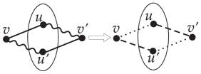
Figure 1: A legal switch.

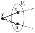
Figure 2: A pairing node.

Finally, notice that $\forall v\in X$ the number of straight and the number of squiggly edges adjacent to $v$ are equal, i.e., they are ${deg_{X}(v)}/{2}$.

Lemma 7.

The Markov chain $\mathcal{M}$ defined above is irreducible.

Proof. By induction on $|E(X)|$. If $|E(X)|=4$, then $X$ has to contain an alternating cycle of length 4, with straight and squiggly edges, with two non adjacent vertices in the same $V_{i}$. Thus we can go from $G$ to $G_{1}$ in one legal switch.

Now assume that $|E(X)|=2k>4$.

Case 1: $X$ contains a pairing node $x$.

Subcase 1a: There exists a straight neighbor of $u$, say $w$, that is also a squiggly neighbor of $v$ (Figure 3a). Then, by switching $[vx,uw|vw,ux]$ in $G$, we reduce $|E(X)|$ to $2k-4$. Thus, by induction, we can go from $G$ to $G_{1}$ by performing a sequence of legal switches.

Subcase 1b: There exists a straight neighbor of $u$, say $w$, that is also a dotted neighbor of $v$, or there exists a dashed neighbor of $u$, $w$, that is also a squiggly neighbor of $v$ (Figure 3b). Then, by switching $[vx,uw|vw,ux]$ in $G$, we reduce $|E(X)|$ to $2k-2$. Thus, by induction, we can go from $G$ to $G_{1}$ by performing a sequence of legal switches.

Subcase 1c: There exists a straight neighbor of $u$, say $w$, that is also a dashed neighbor of $v$, or there exists a dotted neighbor of $u$, $w$, that is also a squiggly neighbor of $v$ (Figure 3c). Notice that by switching $[ux,vw|uw,vx]$ in $G_{1}$, we get a graph $G_{1}^{\prime}$, such that $|E(G\oplus G_{1}^{\prime})|=2k-2$. Thus, by induction, we can go from $G$ to $G_{1}^{\prime}$ by performing a sequence of legal switches. Then, by switching $[ux,vw|uw,vx]$ in $G_{1}^{\prime}$, we get $G_{1}$.

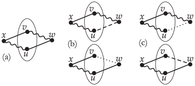
Figure 3: Case 1.

Now, we claim that always one of the above subcases holds. Assume not. That is, (i) all straight neighbors of $u$ ($v$ excluded) are also straight neighbors of $v$ and (ii) all squiggly neighbors of $v$ ($u$ excluded) are also squiggly neighbors of $u$. Since, $x$ is a squiggly neighbor of $u$ and a straight neighbor of $v$, (i) implies that $deg_{X}(u)/2<deg_{X}(v)/2$ (Figure 4a) and (ii) implies that $deg_{X}(u)/2>deg_{X}(v)/2$ (Figure 4b), producing a contradiction.

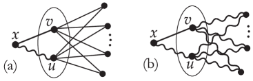
Figure 4: Subcases 1a, 1b, and 1c exhaust all possibilities for Case 1.

Case 2: $X$ contains no pairing node.

Then, there exist two edges, one squiggly $xu$ and one straight $yv$ such that $u,v,x,y$ are all distinct and $x,y\in V_{i}$, $u,v\in V_{j}$ for some $i,j$ (Figure 5).

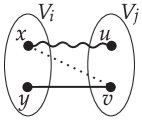
Figure 5: If no pairing node exists.

Notice that $xv$ can only be either dashed or dotted. Assume it is dotted. (The case where $xv$ is dashed is symmetric.) Then, $v$ is a neighbor of $y$ in $G$, but not of $x$. Since $x$ and $y$ have the same degree in $G$, there exists some $w$ such that $xw$ is in $E(G)$, while $yw$ is not.

Subcase 2a: The edge $xw$ is straight and $yw$ is dotted. Then, by switching $[xw,yv|xv,yw]$ in $G$, we keep $|E(X)|=2k$ and we create the pairing node $x$ (Figure 6a). By Case 1 above and induction, we can go from $G$ to $G_{1}$ by performing a sequence of legal switches.

Subcase 2b: The edge $xw$ is dashed and $yw$ is squiggly. Like above, by switching $[xw,yv|xv,yw]$ in $G$, we keep $|E(X)|=2k$ and we create the pairing node $x$ (Figure 6b). By Case 1 above and induction, we can go from $G$ to $G_{1}$ by performing a sequence of legal switches.

Subcase 2c: The edge $xw$ is dashed and $yw$ is dotted. Then, by switching $[xw,yv|xv,yw]$ in $G$, we have $|E(X)|=2k+2$ and we create two pairing nodes $x,w$ (Figure 6c). By examining the pairing node $x$ with $u,v$ like we did in subcases 1a, 1b, 1c above, we either reduce $|E(X)|$ to $2k-2$ and proceed with induction, or we reduce $|E(X)|$ to $2k$, while $X$ has the pairing node $w$, in which case, by Case 1 above and induction, we can go from $G$ to $G_{1}$ by performing a sequence of legal switches.

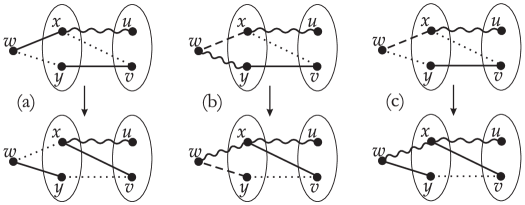
Figure 6: Subcases 2a, 2b, and 2c

Notice that in Case 2, it is not possible to have $xw$ to be straight and $yw$ to be squiggly.

$\boxdot$

5 Further Directions

For the original degree sequence graphic realization problem, when a graphic realization of a degree sequence $d_{1}\geq d_{2}\geq\ldots\geq d_{n}$ exists, several interesting generalizations can be solved efficiently. For example, if there are costs on edges, then we can find a minimum cost realization and we can generate a realization, or a connected realization uniformly at random (under mild restrictions on the degree sequence [22, 19, 8, 17]).

The above problems have efficient algorithms because the original problem has a reduction to perfect matchings [33, 22, 31]. In particular, for $d_{1}\geq d_{2}\geq\ldots\geq d_{n}$ as above, define the graph ${\cal G}\!=\!({\cal V},{\cal E})$ as follows. The vertex set is ${\cal V}\!=\!\cup_{i=1}^{n}V_{i}$, where $V_{i}\!=\!\cup_{j\in[n],j\neq i}\{v_{ij}\}\cup_{j^{\prime}=1}^{n-d_{i}-1}\{u_{ij^{\prime}}\}$, $\forall 1\leq i\leq n$. The vertices $v_{ij}$ denote a potential edge between $i$ and $j$ in the graphic realization. The vertices $u_{ij^{\prime}}$ will enforce the required degrees $d_{i}$. Now the edges are ${\cal E}\!=\!\cup_{1\leq i<j\leq n}\{\{v_{ij},v_{ji}\}\}\cup_{i=1}^{n}\cup_{j=1}^{n-1}\cup_{j^{\prime}=1}^{n-d_{i}-1}\{\{v_{ij},u_{ij^{\prime}}\}\}$. It is straightforward to verify that the degree sequence is realizable if and only if ${\cal G}$ has a perfect matching.

Is there a reduction from the joint-degree matrix realization problem to some version of matching, flow, or a similar better understood combinatorial problem? The relatively smooth decision and construction algorithm outlined in Section 2 for realizability suggests that such a reduction might exist. One should probably try to reverse engineer the construction algorithm; however, the main difficulty is outlined in Remark 1 at the end of Section 2, namely, the alternating sequences of edges involved in the algorithm are not pure augmenting paths. The existence of a such a reduction may help solve the problems listed in the next paragraph.

The most interesting open question is undoubtedly whether one can efficiently sample from $\langle{\mathbb{V}},d,D\rangle$. It would be interesting to prove that the Markov chain we suggest in Section 4, or any other Markov chain for that matter, is rapid mixing. Although some progress has been made in this direction in [15], the problem remains largely open. Similar questions can be asked for a weighted version of the problem. Let $\langle{\mathbb{V}},d,D\rangle$ be an instance of the joint-degree matrix realization problem. If there is a cost associated with every potential edge, can we construct a realization of minimum cost? More importantly, can we generate uniformly at random such a realization?

It is also natural to define the following generalization of the graphic realization problem, where conditions on the number of edges involve arbitrary subsets of vertices. In particular, for $V=[n]$ and positive integers $d_{1}\geq d_{2}\geq\ldots\geq d_{n}$, let ${\mathbb{S}}=\{S_{1},S_{2},\ldots,S_{k}\}$ be an arbitrary partition of $V$, and let $D\!=\!(d_{ij})$, $1\leq i\leq j\leq k$, be a $k\times k$ matrix, where $d_{ij}$ is the number of edges between $S_{i}$ and $S_{j}$. As is, this is the same as the partition adjacency matrix problem introduced in [9], and the skeleton graph problem introduced in [13], where some special cases are studied. Is there a polynomial decision/construction algorithm for the above problem in general? Notice that this is not a direct generalization of the joint-degree matrix problem, as was noted in [13], unless we modify the above definition to specify the degree subsequences in each $S_{i}$.

References

- [1] W. Aiello, F. Chung, and L. Lu. Random evolution in massive graphs. FOCS, 2000.
- [2] W. Aiello, F. Chung, and L. Lu. A random graph model for massive graphs. STOC, 2000.
- [3] D. Alderson, J. Doyle, R. Govindan, and W. Willinger. Toward an optimization-driven framework for designing and generating realistic internet topologies. ACM Sigcomm CCR, 2003.
- [4] A. Barabasi. Linked: The New Science of Networks. NY Perseus, 2002.
- [5] C. Berge. Graphs and Hypergraphs. North Holland Publishing Company, 1973.
- [6] K. Calvert, M. Doar, and E.W. Zegura. Modeling internet topology. IEEE Communications Magazine, 1997.
- [7] F. Chung and L. Lu. Complex Graphs and Networks. AMS, 2004.
- [8] C. Cooper, M. Dyer, and C. Greenhill. Sampling regular graphs and a p2p network. SODA, 2005.
- [9] É. Czabarka. On realizations of a Partition Adjacency Matrix. Unpublished Manuscript, 2014.
- [10] É. Czabarka, A. Dutle, P. L. Erdős, and I. Miklós. On realizations of a joint degree matrix. Discrete Applied Mathematics, 181:283 – 288, 2015.
- [11] S. N. Dorogovetisev and J. F. F. Mendes. Evolution of Networks: from Biological Nets to the Internet and WWW. Oxford University Press, 2003.
- [12] R. Durrett. Random Graph Dynamics. Cambridge U. Press, 2006.
- [13] P. L. Erdős, S. G. Hartke, L. van Iersel, and I. Miklós. Graph realizations constrained by skeleton graphs. ArXiv e-prints: 1508.00542, 2015.
- [14] P. Erdős and T. Gallai. Graphs with prescribed degrees of vertices. Math. Lapok, 11, 1960.
- [15] P. L. Erdős, I. Miklós, and Z. Toroczkai. A decomposition based proof for fast mixing of a markov chain over balanced realizations of a joint degree matrix. SIAM Journal on Discrete Mathematics, 29(1):481–499, 2015.
- [16] M. Faloutsos, P. Faloutsos, and C. Faloutsos. On power-law relationships of the internet topology. Sigcomm, 1999.
- [17] T. Feder, A. Guetz, M. Mihail, and A. Saberi. A local exchange markov chain on graphs with given degrees and applications in p2p networks. FOCS, 2006.
- [18] M. Gjoka, B. Tillman, and A. Markopoulou. Construction of simple graphs with a target joint degree matrix and beyond. In 2015 IEEE Conference on Computer Communications (INFOCOM), pages 1553–1561, 2015.
- [19] C. Gkantsidis, M. Mihail, and E. Zegura. The markov chain simulation method for generating connected power law random graphs. ALENEX (SODA Workshop), 2003.
- [20] S.L. Hakimi. On the realizability of a set of integers as degrees of the vertices of a graph. SIAM, J. Applied Math., 10, 1960.
- [21] V. Havel. A remark on the existence of finite graphs. Kaposis Pest Mat, 80, 1955.
- [22] M. Jerrum and A. Sinclair. Fast uniform generation of regural graphs. TCS, 73, 1990.
- [23] C. Jin, Q. Chen, and S. Jamin. Inet: Internet topology generator, http://irl.eecs.umich.edu/jamin. University of Michigan technical Report, CSE-TR-433-00, 2000.
- [24] L. Li, D. Alderson, W. Willinger, and J. Doyle. A first-principles approach to understanding the internet’s router level topology. Sigcomm, 2004.
- [25] P. Mahadevan, D. Krioukov, K. Fall, and A. Vahdat. Systematic topology analysis and generation using degree correlations. Sigcomm, 2006.
- [26] P. Mahadevan, D. Krioukov, M. Fomenkov, B. Huffaker, X. Dimitropoulos, kc claffy, and A. Vahdat. The internet as-topology: Three data sources and a definitive metric. ACM Sigcomm CCR, 2006.
- [27] A. Medina, I. Matta, and J. Byers. On the origin of power laws in internet topologies. ACM Sigcomm CCR, 2000.
- [28] M. Newman. Assortative mixing in networks. Phys. Rev. Lett. 89, 2002.
- [29] M. Newman. Mixing patterns in networks. Phys. Rev. Lett. E 67, 2003.
- [30] M. Newman, Barabasi A.L., and D. Watts. The Structure and Dynamics of Networks. Princeton U. Press, 2006.
- [31] A. Sinclair. Algorithms for Random Generation and Counting: A Markov Chain Approach. Springer-Verlag, 1997.
- [32] I. Stanton and A. Pinar. Constructing and sampling graphs with a prescribed joint degree distribution. J. Exp. Algorithmics, 17:3.5:3.1–3.5:3.25, September 2012.
- [33] L. Valiant. The complexity of enumeration and reliability problems. SIAM, J. Computing, 8, 1979.
- [34] E. W. Zegura, Ken Calvert, and S. Bhattacharjee. How to model an internetwork. In Infocom, 1996.