Bifurcation of soliton families from linear modes in non-$\mathcal{PT}$-symmetric complex potentials

Abstract

Continuous families of solitons in generalized nonlinear Schödinger equations with non-$\mathcal{PT}$-symmetric complex potentials are studied analytically. Under a weak assumption, it is shown that stationary equations for solitons admit a constant of motion if and only if the complex potential is of a special form $g^{2}(x)+ig^{\prime}(x)$, where $g(x)$ is an arbitrary real function. Using this constant of motion, the second-order complex soliton equation is reduced to a new second-order real equation for the amplitude of the soliton. From this real soliton equation, a novel perturbation technique is employed to show that continuous families of solitons always bifurcate out from linear discrete modes in these non-$\mathcal{PT}$-symmetric complex potentials. All analytical results are corroborated by numerical examples.

1 Introduction

Nonlinear wave systems fall into two major categories: conservative and dissipative. Conservative systems are energy-conserving, and their solitary waves (solitons) exist as continuous families with continuous ranges of energy values. A typical example is the nonlinear Schrödinger (NLS) equation. Dissipative systems contain gain and loss, and their solitons are generally isolated with certain discrete energy values. A typical example of this type is the Ginzburg-Landau equation. A recent discovery is that, in dissipative but parity-time ($\mathcal{PT}$) symmetric systems, solitons can still exist as continuous families with continuous energy values [2, 3, 4, 5, 6, 7, 8, 9, 10, 11, 12, 13, 14, 15, 16, 17, 18, 19, 20]. An example in this category is the NLS equation with a complex but $\mathcal{PT}$-symmetric potential. These soliton families are allowed since the $\mathcal{PT}$symmetry assures that the gain and loss of the soliton is perfectly balanced at arbitrary energy levels.

In dissipative and non-$\mathcal{PT}$-symmetric systems, the expectation is that any solitons will be isolated with discrete energy values, as seen in typical dissipative systems [21]. However, exceptions were reported numerically in [22, 23] for the NLS equation with a non-$\mathcal{PT}$-symmetric complex potential of special form, where families of solitons with continuous energy values can bifurcate out from the linear modes of the potential. This finding is very surprising in view of the lack of $\mathcal{PT}$symmetry here. For these special potentials, a constant of motion was discovered in [23] for the stationary soliton equation. Using this constant of motion, soliton families in these special potentials were explained by a numerical shooting argument [23].

In this article, we analytically investigate solitons of the NLS equation with non-$\mathcal{PT}$-symmetric complex potentials. We focus on three main questions: (1) What types of non-$\mathcal{PT}$-symmetric complex potentials admit soliton families? (2) How can one analytically explain and calculate soliton families bifurcating from linear modes in such potentials? (3) Do these soliton families exist under other nonlinearities?

Regarding the first question, we recognize that in the absence of $\mathcal{PT}$symmetry, the existence of a constant of motion in the stationary soliton equation plays a crucial role in the existence of soliton families. Assuming this constant of motion for complex potentials is a continuous deformation of one that exists in the NLS equation without a potential, we show that the only complex potentials which admit a constant of motion are those of the form reported in [22, 23], i.e., $V(x)=g^{2}(x)+ig^{\prime}(x)$, where $g(x)$ is an arbitrary real function. This strongly suggests that potentials of the above form are the only one-dimensional non-$\mathcal{PT}$-symmetric complex potentials that admit soliton families.

On the second question, through use of the constant of motion, we reduce the second-order complex soliton equation to a new second-order real equation for the square of amplitude of the soliton, which is then solved perturbatively for a continuous range of $\mu$ values. This way, the existence of soliton families bifurcating from linear modes in non-$\mathcal{PT}$-symmetric potentials is analytically explained and explicitly calculated. Interestingly, this perturbation calculation of solitons differs significantly from the method used for real and $\mathcal{PT}$-symmetric potentials because the linearization operator of the new real equation has a distinctly different kernel structure.

Regarding the third question, we show that these soliton families still exist under a more general class of nonlinearities. Furthermore, the choice of nonlinearity within this class has no effect on the existence of a constant of motion.

These analytical results are compared with numerical examples, and good agreement between them is illustrated.

2 Preliminaries

The mathematical model we consider, in most parts of this article, is the NLS equation with a complex potential,

$$i\Psi_{t}+\Psi_{xx}+V(x)\Psi+\sigma|\Psi|^{2}\Psi=0,$$ (1)

where $\sigma=\pm 1$ is the sign of cubic nonlinearity. This model describes paraxial nonlinear light propagation in a waveguide with gain and loss [3, 24], as well as Bose-Einstein condensates with atoms injected into one part of the potential and removed from another part of the potential [25, 26]. Most of the earlier work focused on the case where the complex potential $V(x)$ is $\mathcal{PT}$-symmetric, i.e., $V^{*}(x)=V(-x)$, with the superscript ‘*’ representing complex conjugation [3, 4, 5, 7, 8, 9, 10]. In this article, we consider the case where $V(x)$ is not $\mathcal{PT}$-symmetric, i.e.,

$$V^{*}(x)\neq V(-x).$$ (2)

Soliton solutions of equation (1) take the form

$$\Psi(x,t)=\psi(x)e^{i\mu t},$$ (3)

where $\psi(x)$ is a localized function solving the stationary equation

$$\psi_{xx}-\mu\psi+V(x)\psi+\sigma|\psi|^{2}\psi=0,$$ (4)

and $\mu$ is a real propagation constant. In $\mathcal{PT}$-symmetric potentials, solitons exist as continuous families parameterized by $\mu$ [4, 5, 7, 8, 9, 10]. But in non-$\mathcal{PT}$-symmetric potentials, soliton families are generically forbidden [21]. Surprisingly, it was reported recently through numerical examples that in complex potentials of the special form

$$V(x)=g^{2}(x)+ig^{\prime}(x),$$ (5)

where $g(x)$ is an arbitrary real function, soliton families can still bifurcate out from linear modes even when $V(x)$ is non-$\mathcal{PT}$-symmetric (i.e., when $g(x)$ is not even) [22, 23]. This result is very unintuitive. Indeed, if one performs a regular perturbation calculation of soliton families bifurcating from linear modes in a general complex potential, it will be seen that infinitely many nontrivial conditions would have to be satisfied simultaneously, which makes such bifurcation almost impossible [21]. However, for the special complex potential (5), all those conditions are met, which is miraculous. Obviously this phenomenon needs better understanding. A step in this direction was made in [23], where through the discovery of a constant of motion for the soliton equation (4) under the potential (5), soliton families in Eq. (4) were explained through a numerical shooting argument.

Many important questions are currently open regarding soliton families in non-$\mathcal{PT}$-symmetric complex potentials. For instance, what other non-$\mathcal{PT}$-symmetric complex potentials admit soliton families? How can one analytically explain and explicitly calculate soliton families bifurcating from linear modes in non-$\mathcal{PT}$-symmetric potentials? Do these soliton families also exist under other nonlinearities? These questions will be investigated in the remainder of this article.

3 Constant of motion

A quantity $J(x,\psi)$ is called a constant of motion in the stationary equation (4) if $dJ/dx=0$. The existence of a constant of motion proves to be important for the existence of soliton families (see [23] and later text). Thus, in this section, we study what complex potentials $V(x)$ admit a constant of motion. In this study, solutions, $\psi(x)$, to the stationary equation (4) are allowed to be any solutions, not necessarily solitons. That is, $\psi(x)$ is allowed to be non-local.

First we split the complex potential $V(x)$ into real and imaginary parts,

$$V(x)=v_{1}(x)+iv_{2}(x),$$ (6)

where $v_{1}(x),v_{2}(x)$ are real functions. We also express the complex function $\psi(x)$ in polar forms,

$$\psi(x)=r(x)e^{i\int\theta(x)dx},$$ (7)

where $r(x)$, $\theta(x)$ are real amplitude and phase functions. Substituting these expressions into the soliton equation (4), we get

$$r_{xx}-\mu r+v_{1}r+\sigma r^{3}-\theta^{2}r=0,$$ (8)

$$(r^{2}\theta)_{x}=-v_{2}r^{2}.$$ (9)

In the absence of the potential ($v_{1}=v_{2}=0$), it is easy to verify that this system admits two constants of motion

$$J_{1}=r^{2}\theta,$$ (10)

and

$$J_{2}=r_{x}^{2}-\mu r^{2}+\frac{\sigma}{2}r^{4}+r^{2}\theta^{2},$$ (11)

where $dJ_{1}/dx=dJ_{2}/dx=0$. Since the system is third order, these are the only constants of motion the system can allow. These two constants of motion are associated with the flux terms of the power and momentum conservation laws of the potential-free NLS equation, but this fact is not important to our analysis.

In the presence of the potential, it is reasonable to assume that the corresponding constant of motion $J$ is a continuous deformation of those in the potential-free case. In other words, $J$ approaches constants of motion of the potential-free equation when $v_{1},v_{2}$ approach zero. Notice that $J_{1}$ and $J_{2}$ have different ranks [27]. Thus under the limit $v_{1},v_{2}\to 0$, $J$ can only approach one of $(J_{1},J_{2})$, not their linear combination. Our strategy then is to calculate $dJ_{k}/dx\>(k=1,2)$ in the presence of the potential and derive conditions on $(v_{1},v_{2})$ so that $dJ_{k}/dx$ is a total derivative of $x$, i.e., a constant of motion is admitted.

Now we calculate $dJ_{k}/dx$ in the presence of a potential. First we consider $dJ_{1}/dx$. Eq. (9) clearly shows that, in order for $dJ_{1}/dx$ to be a total derivative, we must have $v_{2}=0$, i.e., the potential $V(x)$ is real. This is not what we want since we exclusively consider complex potentials in this paper. Thus, there are no constants of motion in Eqs. (8)-(9) that approach $J_{1}$ when the complex potential approaches zero.

Next we consider $dJ_{2}/dx$. Utilizing equations (8)-(9), we readily find that

$$\frac{dJ_{2}}{dx}=-v_{1}(r^{2})_{x}-2v_{2}r^{2}\theta.$$ (12)

The right side of this equation can be rewritten as

$$\frac{dJ_{2}}{dx}=W_{x}+r^{2}v_{1x}+2(r^{2}\theta)_{x}\int v_{2}dx,$$ (13)

where

$$W=-v_{1}r^{2}-2r^{2}\theta\int v_{2}dx.$$

Then utilizing equation (9), the above equation becomes

$$\frac{dJ_{2}}{dx}=W_{x}+r^{2}\left(v_{1x}-2v_{2}\int v_{2}dx\right).$$ (14)

In order for the right side of the above equation to be a total derivative, the necessary and sufficient condition is

$$v_{1x}=2v_{2}\int v_{2}dx.$$ (15)

This condition can be rewritten as

$$v_{1x}=\left[\left(\int v_{2}dx\right)^{2}\right]_{x},$$ (16)

thus

$$v_{1}=\left(\int v_{2}dx\right)^{2}+C,$$ (17)

where $C$ is an arbitrary constant. Finally, denoting

$$g=\int v_{2}dx,$$ (18)

the potential $V(x)$ which admits a constant of motion then is of the form

$$V(x)=g^{2}(x)+ig^{\prime}(x)+C.$$ (19)

Obviously, the constant $C$ in this potential can be eliminated from Eq. (1) through a simple gauge transformation. The remaining potential is then of the form (5). Thus we conclude that if the constant of motion for the stationary equation (4) with a complex potential is a continuous deformation of $J_{2}$ without the potential, then this constant of motion exists if and only if the complex potential $V(x)$ is of the special form (5), and the corresponding motion constant is

$$J=J_{2}-W=J_{2}+g^{2}r^{2}+2gr^{2}\theta,$$ (20)

or more explicitly,

$$J=r_{x}^{2}-\mu r^{2}+\frac{\sigma}{2}r^{4}+r^{2}(\theta+g)^{2},$$ (21)

where $dJ/dx=0$. This constant of motion agrees with that reported in [23] for these special potentials (5).

4 Bifurcation of soliton families

In this section, we analytically calculate the bifurcation of solitons from linear modes in Eq. (1), with potential of the special form (5), and show that soliton families bifurcate out in such non-$\mathcal{PT}$-symmetric systems.

For the potential (5), when solitons (3) are expressed in polar forms (7), the equations for $r$ and $\theta$ are seen from Eqs. (8)-(9) as

$$r_{xx}-\mu r+g^{2}r+\sigma r^{3}-\theta^{2}r=0,$$ (22)

$$(r^{2}\theta)_{x}=-g_{x}r^{2},$$ (23)

and these equations admit a constant of motion (21). For solitons, this constant $J$ can be evaluated at $x=\infty$ as zero, thus

$$r_{x}^{2}-\mu r^{2}+\frac{\sigma}{2}r^{4}+r^{2}(\theta+g)^{2}=0.$$ (24)

From this equation, we get

$$\theta=-g\pm\sqrt{\mu-\frac{1}{2}\sigma r^{2}-\frac{r_{x}^{2}}{r^{2}}}.$$ (25)

Inserting it into Eq. (22) and after simple algebra, we get

$$r_{xx}-2\mu r+\frac{3}{2}\sigma r^{3}+\frac{r_{x}^{2}}{r}=\mp 2g\sqrt{\mu r^{2}-\frac{1}{2}\sigma r^{4}-r_{x}^{2}},$$ (26)

or

$$(r^{2})_{xx}-4\mu r^{2}+3\sigma r^{4}\pm 2g\sqrt{4\mu r^{4}-2\sigma r^{6}-[(r^{2})_{x}]^{2}}=0.$$ (27)

Denoting $R=r^{2}$, we arrive at a single second-order equation for the real amplitude function $R$ as

$$R_{xx}-4\mu R+3\sigma R^{2}\pm 2g\sqrt{4\mu R^{2}-2\sigma R^{3}-R_{x}^{2}}=0,$$ (28)

which can also be rewritten as

$$\left(\sqrt{4\mu R^{2}-2\sigma R^{3}-R_{x}^{2}}\right)_{x}=\pm 2gR_{x}.$$ (29)

4.1 Perturbation calculations

The sign in Eq. (28) needs to be chosen appropriately according to the function $g(x)$. Indeed, if $g(x)$ switches to $-g(x)$, this sign should switch as well. Without loss of generality, we take the plus sign in Eq. (28),

$$R_{xx}-4\mu R+3\sigma R^{2}+2g\sqrt{4\mu R^{2}-2\sigma R^{3}-R_{x}^{2}}=0.$$ (30)

Note that sometimes the same solution $R(x)$ can lead to mixed signs in Eq. (28) on different $x$-intervals. This could occur if $4\mu R^{2}-2\sigma R^{3}-R_{x}^{2}$ is zero somewhere on the $x$-axis, since the square root is a possible mechanism for inducing a sign change so that the square-rooted quantity remains smooth. We do not consider such mixed cases here. This exclusion will be assured by Assumption 1 in Sec. 4.3.

For a localized function $g(x)$, it is easy to see that the large-$x$ asymptotics of the soliton solution in Eq. (30) are, to leading order,

$$R(x)\to a_{\pm}e^{-\sqrt{4\mu}|x|},\quad x\to\pm\infty,$$ (31)

where $a_{\pm}$ are positive constants.

First we consider linear modes in Eq. (30), which satisfy the equation

$$\phi_{xx}-4\mu_{0}\phi+2g\sqrt{4\mu_{0}\phi^{2}-\phi_{x}^{2}}=0.$$ (32)

This equation can be rewritten as

$$\left(\sqrt{4\mu_{0}\phi^{2}-\phi_{x}^{2}}\right)_{x}=2g\phi_{x}.$$ (33)

Since $g$ and $\phi$ are localized functions, we see that

$$\sqrt{4\mu_{0}\phi^{2}-\phi_{x}^{2}}=\int_{-\infty}^{x}2g\phi_{\xi}d\xi=-\int_{x}^{\infty}2g\phi_{\xi}d\xi,$$ (34)

and

$$\int_{-\infty}^{\infty}2g\phi_{\xi}d\xi=0.$$ (35)

Equation (32) is scaling-invariant and thus an eigenvalue problem, but it is nonlinear in both the eigenvalue $\mu_{0}$ and eigenfunction $\phi$. Thus, this is a different type of eigenvalue problem. Solving this new eigenvalue problem is equivalent to solving for discrete real eigenmodes in the original eigenvalue problem from Eq. (4), i.e.,

$$\psi_{xx}+V(x)\psi=\mu_{0}\psi,$$ (36)

and the eigenfunction correspondence is $\phi=|\psi|^{2}$. Previous results in [22] have shown that for the underlying special potential (5), the linear eigenvalue problem (36) admits discrete real eigenvalues for a large class of functions $g(x)$. The new eigenvalue problem (32) makes the existence of such real eigenvalues more clear since all quantities in that equation are real.

From such eigenmodes, families of solitons can bifurcate out under variation of $\mu$. We will analytically prove this by explicitly calculating this soliton bifurcation from a linear mode $(\mu_{0},\phi)$ using perturbation methods.

The perturbation expansion is

$$R = \epsilon(R_{0}+\epsilon R_{1}+\epsilon^{2}R_{2}+\dots),$$ (37)

$$\mu = \mu_{0}+\epsilon,$$ (38)

where $\epsilon>0$ is a small parameter. Here we have assumed the bifurcation occurs to the right side of $\mu_{0}$. As we will see later, this assumption dictates the sign of nonlinearity $\sigma$. If the bifurcation occurs to the left side of $\mu_{0}$, then only trivial modifications to our analysis are needed, and the bifurcation will occur for the opposite sign of nonlinearity.

Inserting the above expansion into Eq. (30), at order $\epsilon$, we find

$$R_{0}=c_{0}\phi,$$ (39)

where $c_{0}$ is a positive constant to be determined.

At order $\epsilon^{2}$, we get

$$LR_{1}=F,$$ (40)

where

$$L=\partial_{xx}+p_{1}\partial_{x}+p_{2},$$ (41)

$$p_{1}=-\frac{2g\phi_{x}}{\sqrt{4\mu_{0}\phi^{2}-\phi_{x}^{2}}},\quad p_{2}=4\mu_{0}\left(\frac{2g\phi}{\sqrt{4\mu_{0}\phi^{2}-\phi_{x}^{2}}}-1\right),$$ (42)

$$F=c_{0}(f_{1}-c_{0}\sigma f_{2}),$$ (43)

and

$$f_{1}=4\phi\left(1-\frac{g\phi}{\sqrt{4\mu_{0}\phi^{2}-\phi_{x}^{2}}}\right),\quad f_{2}=\phi^{2}\left(3-\frac{2g\phi}{\sqrt{4\mu_{0}\phi^{2}-\phi_{x}^{2}}}\right).$$ (44)

Now it is time to analyze the properties of homogeneous solutions and adjoint homogeneous solutions of the operator $L$ and the solvability condition of Eq. (40).

4.2 Kernels of linearization operators $L$ and $L^{A}$

First, it is easy to verify that $\phi$ is a homogeneous solution of $L$, i.e.,

$$L\phi=0.$$ (45)

Let us suppose the other homogeneous solution of $L$ is $\phi_{2}$, then according to Abel’s formula, the Wronskian of $(\phi,\phi_{2})$ is

$$W(\phi,\phi_{2})=W_{0}e^{-\int p_{1}dx},$$ (46)

or

$$W(\phi,\phi_{2})=W_{0}\sqrt{4\mu_{0}\phi^{2}-\phi_{x}^{2}}$$ (47)

in view of Eqs. (33) and (42). Here $W_{0}$ is a constant. Utilizing Eq. (34), the above Wronskian can be rewritten as

$$W(\phi,\phi_{2})=W_{0}\int_{-\infty}^{x}2g\phi_{\xi}d\xi=-W_{0}\int_{x}^{\infty}2g\phi_{\xi}d\xi.$$ (48)

From this formula we see that, if $g(x)$ is a localized function, then the decay rate of this Wronskian at large $|x|$ is faster than that of $\phi$, and thus $\phi_{2}$ is also a localized function.

Using these homogeneous solutions of $L$, we can build homogeneous solutions of the adjoint operator $L^{A}$, where

$$L^{A}=\partial_{xx}-\partial_{x}p_{1}+p_{2}.$$ (49)

Lemma 1 The two homogeneous solutions $(\phi^{A},\phi_{2}^{A})$ of adjoint operator $L^{A}$ are

$$\phi^{A}=-\frac{\phi_{2}}{W(\phi,\phi_{2})},\quad\phi_{2}^{A}=\frac{\phi}{W(\phi,\phi_{2})}.$$ (50)

Proof: We first turn the second-order homogeneous equation of operator $L$ into a system of first-order equations,

$$X^{\prime}=\left[\begin{array}[]{cc}0&1\\ -p_{2}&-p_{1}\end{array}\right]X,$$ (51)

where the prime stands for derivative to $x$. The fundamental matrix solution to this system is

$$X=\left[\begin{array}[]{cc}\phi&\phi_{2}\\ \phi_{x}&\phi_{2x}\end{array}\right].$$ (52)

The adjoint system of Eq. (51) is

$$Y^{\prime}=-\left[\begin{array}[]{cc}0&-p_{2}\\ 1&-p_{1}\end{array}\right]Y.$$ (53)

Notice that if $Y=[y_{1},y_{2}]^{T}$, where the superscript ‘$T$’ represents vector or matrix transpose, then it is easy to verify that

$$L^{A}y_{2}=0,$$ (54)

i.e., the second component of vector solution $Y$ is in the kernel of the adjoint operator $L^{A}$.

It is well known that the fundamental matrix solution to the adjoint vector system (53) is $\left(X^{-1}\right)^{T}$. This can be proved by calculating $(XX^{-1})^{\prime}$, where upon utilizing Eq. (51), a homogeneous differential equation for $X^{-1}$ would be obtained. Taking the transpose of this equation would reveal that $\left(X^{-1}\right)^{T}$ satisfies the adjoint equation (53). Notice that

$$\left(X^{-1}\right)^{T}=\frac{1}{W(\phi,\phi_{2})}\left[\begin{array}[]{cc}\phi_{2x}&-\phi_{x}\\ -\phi_{2}&\phi\end{array}\right].$$ (55)

Since the second-row functions in this matrix are in the kernel of the adjoint operator $L^{A}$, the functions $\phi^{A}$ and $\phi_{2}^{A}$ defined in Eq. (50) are then homogeneous solutions of the adjoint operator $L^{A}$. $\Box$

In view of Lemma 1, if $g(x)$ is a localized function, then both adjoint homogeneous solutions $\phi^{A},\phi_{2}^{A}$ are unbounded, because the decay rates of $\phi$ and $\phi_{2}$ at large $|x|$ are slower than that of the Wronskian $W(\phi,\phi_{2})$.

The fact that $L$ has only localized solutions and $L^{A}$ has only unbounded solutions in their kernels makes the solvability condition for the first-order equation (40) novel, as we will delineate below.

4.3 Solvability conditions for certain potentials

In this subsection, we show how to impose the solvability condition on Eq. (40) under the following assumptions.

Assumption 1  For the linear eigenmode $(\mu_{0},\phi)$, $4\mu_{0}\phi^{2}-\phi_{x}^{2}$ is strictly positive for all $x$;

Assumption 2  The function $g(x)$ decays exponentially at large $x$ as

$$g(x)\to b_{\pm}e^{-\beta|x|},\quad x\to\pm\infty,$$ (56)

where $b_{\pm}$ and $\beta>0$ are constants.

Assumption 3 For these potentials, $\sqrt{4\mu_{0}}>\beta$.

Assumption 1 assures that the linear operators $L,L^{A}$ are nonsingular. In addition, there will be no sign change on the $x$-interval in Eq. (28). This assumption will be made throughout the text.

Assumptions 2 and 3 are introduced in order to make our analysis more explicit. If the function $g(x)$ does not satisfy these assumptions, an alternative analysis will be outlined in the next subsection.

Remark 1   In some sense Assumptions 2 and 3 represent the most common case, since for practical purposes the exact decay rate at large $x$ should have minimal effect on the dynamics of the system. Hence modifying the small tails of the potential to have a suitably exponentially decaying rate should not make a meaningful difference. However, we will still show in the next subsection that these perturbation calculations may be performed for general potentials, and then verify all results numerically.

At large $|x|$, the asymptotics of the eigenfunction $\phi(x)$ can be readily seen from Eq. (32) as

$$\phi(x)\to\gamma_{\pm}e^{-\sqrt{4\mu_{0}}|x|},\quad x\to\pm\infty,$$ (57)

where $\gamma_{\pm}$ are constants. Then under Assumption 2, it is easy to see from Eqs. (34) that the large-$x$ asymptotics of $\sqrt{4\mu_{0}\phi^{2}-\phi_{x}^{2}}$ is

$$\sqrt{4\mu_{0}\phi^{2}-\phi_{x}^{2}}\to s_{\pm}e^{-(\beta+\sqrt{4\mu_{0}})|x|},\quad x\to\pm\infty,$$ (58)

where

$$s_{\pm}=\frac{2b_{\pm}\gamma_{\pm}\sqrt{4\mu_{0}}}{\beta+\sqrt{4\mu_{0}}}.$$

Thus

$$p_{1}(x)\to\pm(\beta+\sqrt{4\mu_{0}}),\quad x\to\pm\infty,$$ (59)

$$p_{2}(x)\to\beta\sqrt{4\mu_{0}},\quad x\to\pm\infty,$$ (60)

hence the asymptotics of operators $L$ and $L^{A}$ are

$$L\to\partial_{xx}\pm(\beta+\sqrt{4\mu_{0}})\partial_{x}+\beta\sqrt{4\mu_{0}},\quad x\to\pm\infty,$$ (61)

and

$$L^{A}\to\partial_{xx}\mp(\beta+\sqrt{4\mu_{0}})\partial_{x}+\beta\sqrt{4\mu_{0}},\quad x\to\pm\infty.$$ (62)

From these asymptotics, it is seen more explicitly that all homogeneous solutions of $L$ are localized (as $e^{-\beta|x|}$, $e^{-\sqrt{4\mu_{0}}|x|}$, or their linear combinations), and all homogeneous solutions of $L^{A}$ are unbounded (as $e^{\beta|x|}$, $e^{\sqrt{4\mu_{0}}|x|}$, or their linear combinations).

Regarding the second homogeneous solution $\phi_{2}(x)$, in view of the asymptotics (57) of the first homogeneous solution $\phi(x)$, without loss of generality we can set the large negative-$x$ asymptotics of $\phi_{2}(x)$ as

$$\phi_{2}(x)\to e^{\beta x},\quad x\to-\infty.$$ (63)

Then its large positive-$x$ asymptotics is

$$\phi_{2}(x)\to\kappa_{1}e^{-\beta x}+\kappa_{2}e^{-\sqrt{4\mu_{0}}x},\quad x\to+\infty,$$ (64)

where $\kappa_{1},\kappa_{2}$ are constants. Substituting these asymptotics into the Wronskian function and using the Wronskian formula (48), the value of $\kappa_{1}$ can be determined. But this $\kappa_{1}$ value is not needed in our analysis.

From Lemma 1 and Eq. (47), we rewrite the adjoint homogeneous solutions $\phi^{A}$ and $\phi_{2}^{A}$ equivalently as

$$\phi^{A}=-\frac{\phi_{2}}{\sqrt{4\mu_{0}\phi^{2}-\phi_{x}^{2}}},\quad\phi_{2}^{A}=\frac{\phi}{\sqrt{4\mu_{0}\phi^{2}-\phi_{x}^{2}}}.$$ (65)

Then using the asymptotics (57), (58), (63) and (64), we find that the large-$x$ asymptotics of $\phi^{A}$ and $\phi_{2}^{A}$ are

$$\phi^{A}(x)\to\left\{\begin{array}[]{ll}-d_{-}e^{-\sqrt{4\mu_{0}}x},&x\to-\infty,\\ -d_{+}\left(\kappa_{1}e^{\sqrt{4\mu_{0}}x}+\kappa_{2}e^{\beta x}\right),&x\to+\infty,\end{array}\right.$$ (66)

and

$$\phi_{2}^{A}(x)\to j_{\pm}e^{\beta|x|},\quad x\to\pm\infty,$$ (67)

where

$$d_{\pm}=\frac{\beta+\sqrt{4\mu_{0}}}{2b_{\pm}\gamma_{\pm}\sqrt{4\mu_{0}}},\quad j_{\pm}=d_{\pm}\gamma_{\pm}.$$ (68)

Notice that both adjoint solutions are unbounded and grow exponentially at large $x$.

The asymptotics of functions $f_{1}$ and $f_{2}$ in the first-order equation (40) can be similarly obtained as

$$f_{1}(x)\to q_{\pm}e^{-\sqrt{4\mu_{0}}|x|},\quad x\to\pm\infty,$$ (69)

and

$$f_{2}(x)\to w_{\pm}e^{-2\sqrt{4\mu_{0}}|x|},\quad x\to\pm\infty,$$ (70)

where

$$q_{\pm}=2\left(1-\frac{\beta}{\sqrt{4\mu_{0}}}\right)\gamma_{\pm},\quad w_{\pm}=\left(2-\frac{\beta}{\sqrt{4\mu_{0}}}\right)\gamma_{\pm}^{2}.$$ (71)

Now we consider the solvability condition of the first-order equation (40). We see from Eqs. (31), (40), (43) and (70) that the large-$x$ asymptotics of $R_{1}(x)$ must be

$$R_{1}(x)\to P_{1}^{\pm}(x)e^{-\sqrt{4\mu_{0}}|x|}+C_{1}^{\pm}e^{-2\sqrt{4\mu_{0}}|x|},\quad x\to\pm\infty,$$ (72)

where $P_{1}^{\pm}(x)$ are certain linear functions of $x$ (these linear functions come about when one expands the tail function $e^{-\sqrt{4\mu}|x|}$ of (31) into a perturbation series around $\mu=\mu_{0}$), and $C_{1}^{\pm}$ are constants. Note that the tails $e^{-2\sqrt{4\mu_{0}}|x|}$ in the above equation are induced by the nonlinearity-related forcing term $f_{2}$ and are admissible. They do not contradict the leading-order $R(x)$ asymptotics (31) since they are of higher order. Enforcement of this tail behavior for $R_{1}(x)$ will yield the solvability condition which determines the $c_{0}$ value.

We begin by taking the inner product of Eq. (40) with $\phi_{2}^{A}(x)$ to get

$$\langle\phi_{2}^{A},LR_{1}\rangle=\langle\phi_{2}^{A},c_{0}(f_{1}-c_{0}\sigma f_{2})\rangle,$$ (73)

where the inner product is defined as

$$\langle f,g\rangle\equiv\int_{-\infty}^{\infty}f^{*}gdx.$$ (74)

Performing integration by parts, the left side of this equation becomes

$$\langle\phi_{2}^{A},LR_{1}\rangle = \langle L^{A}\phi_{2}^{A},R_{1}\rangle+\left.\left(\phi_{2}^{A}R_{1x}-\phi_{2x}^{A}R_{1}+p_{1}\phi_{2}^{A}R_{1}\right)\right|_{-\infty}^{+\infty}$$ (75)

$$= \left.\left(\phi_{2}^{A}R_{1x}-\phi_{2x}^{A}R_{1}+p_{1}\phi_{2}^{A}R_{1}\right)\right|_{-\infty}^{+\infty}.$$

In view of the asymptotics of $\phi_{2}^{A},R_{1}$ and $p_{1}$ in Eqs. (59), (67) and (72), as well as Assumption 3, we see that the right side of the above equation is zero, hence we obtain a solvability condition from Eq. (73) as

$$\langle\phi_{2}^{A},f_{1}-c_{0}\sigma f_{2}\rangle=0.$$ (76)

This solvability condition is the analog of Fredholm Alternatives condition, and it quickly yields the formula for $c_{0}$ as

$$c_{0}=\frac{\langle\phi_{2}^{A},f_{1}\rangle}{\sigma\langle\phi_{2}^{A},f_{2}\rangle}.$$ (77)

Notice that $f_{1}$ and $f_{2}$ decay at large $x$ as $e^{-\sqrt{4\mu_{0}}|x|}$ or faster [see Eqs. (69)-(70)], and $\phi_{2}^{A}(x)$ grows at large $x$ as $e^{\beta|x|}$ [see (67)]. Thus under Assumption 3, both integrals in the inner products of the above equation converge, and hence $c_{0}$ is well defined.

Eq. (77) is a necessary condition for the existence of the first-order solution $R_{1}(x)$ with suitable asymptotics (72). Since $c_{0}$ must be positive, Eq. (77) then shows that, in order for the soliton bifurcation to occur to the right side of $\mu_{0}$ [see Eq. (38)], the sign of nonlinearity $\sigma$ must be chosen as the sign of the ratio $\langle\phi_{2}^{A},f_{1}\rangle/\langle\phi_{2}^{A},f_{2}\rangle$.

The above solvability condition (77) turns out to be also sufficient for the existence of solution $R_{1}(x)$ with suitable asymptotics (72). To show this, we notice that the general solution to the first-order equation (40) can be derived by variation of parameters as

$$R_{1}(x)=\phi(x)\int_{0}^{x}\phi^{A}(\xi)F(\xi)d\xi+\phi_{2}(x)\int_{0}^{x}\phi_{2}^{A}(\xi)F(\xi)d\xi+c_{1}\phi(x)+c_{2}\phi_{2}(x),$$ (78)

where $c_{1}$ and $c_{2}$ are real constants. Using the asymptotics detailed earlier in this section and under Assumption 3, we find that at large $x$, $\phi^{A}(x)F(x)$ approaches a constant, and $\phi_{2}^{A}(x)F(x)$ decays exponentially. Thus

$$\int_{0}^{x}\phi^{A}(\xi)F(\xi)d\xi\to\widetilde{P}_{1}^{\pm}(x),\quad x\to\pm\infty,$$ (79)

where $\widetilde{P}_{1}^{\pm}(x)$ are linear functions of $x$, and

$$\int_{0}^{x}\phi_{2}^{A}(\xi)F(\xi)d\xi\to\int_{0}^{\pm\infty}\phi_{2}^{A}(\xi)F(\xi)d\xi,\quad x\to\pm\infty.$$ (80)

In view of the large-$x$ asymptotics of $\phi(x)$ and $\phi_{2}(x)$, in order for $R_{1}(x)$ in (78) to exhibit the suitable asymptotics (72), the necessary and sufficient conditions are

$$\int_{0}^{\pm\infty}\phi_{2}^{A}(\xi)F(\xi)d\xi+c_{2}=0,$$ (81)

which leads to the equation

$$\int_{-\infty}^{+\infty}\phi_{2}^{A}(x)F(x)dx=0.$$ (82)

Substituting the expression (43) for $F(x)$ into this equation, we then obtain the $c_{0}$ formula (77). Hence this $c_{0}$ formula is a necessary and sufficient condition for the existence of solution $R_{1}(x)$ with suitable asymptotics (72).

In the $R_{1}$ formula (78), while $c_{0}$ is given by formula (77) and $c_{2}$ given by equation (81), $c_{1}$ is still a free parameter. This $c_{1}$ parameter will be fixed by requiring the second-order solution $R_{2}(x)$ to have suitable large-$x$ asymptotics [similar to (72) but with linear functions $P_{1}^{\pm}(x)$ replaced by quadratic functions $P_{2}^{\pm}(x)$]. This calculation of $c_{1}$ is in the same spirit of the $c_{0}$ calculation, thus details will not be pursued in this article.

4.4 Extension to general potentials

In the event that Assumptions 2 and 3 of the previous subsection do not hold, i.e., the decay rate of the potential is not simply exponential, or the exponential decay rate is too fast, i.e. $\beta>\sqrt{4\mu_{0}}$, then the simple $c_{0}$ formula (77) in the previous subsection will be invalid. For instance, when $\beta>\sqrt{4\mu_{0}}$, the integral in the numerator of (77) would be divergent in view of the asymptotics of its integrand. The quantity on the right side of Eq. (75) would not vanish either. Thus the solvability condition for these more general potentials needs a different treatment.

In our new treatment, we consider the $R_{1}(x)$ solution (78) and demand that its tail asymptotics match (72). In particular, this entails choosing $c_{0}$ such that the terms of which decay like $g(x)$ ($e^{-\beta|x|}$ for exponential potentials) are eliminated.

Suppose the tail asymptotics of the second homogenous solution $\phi_{2}(x)$ has the form

$$\phi_{2}\rightarrow\left\{\begin{array}[]{c c}\tau^{-}(x),&x\rightarrow-\infty,\\ \kappa_{2}e^{-\sqrt{4\mu_{0}}x}+\tau^{+}(x),&x\rightarrow+\infty,\end{array}\right.$$ (83)

where $\kappa_{2}$ is a certain real constant, and $\tau^{\pm}(x)$ are the other decaying tail functions. This $\phi_{2}$ asymptotics is the counterpart of Eqs. (63)-(64) in the previous subsection.

We substitute the $F$ formula (43) into (78). Then this $R_{1}$ solution can be rewritten as

$$R_{1}(x)=c_{0}\left[R_{11}(x)-c_{0}\sigma R_{12}(x)\right]+c_{1}\phi(x)+c_{2}\phi_{2}(x),$$ (84)

where $R_{11}(x)$ and $R_{12}(x)$ are particular solutions of equations

$$LR_{11}(x)=f_{1},\quad LR_{12}(x)=f_{2}.$$ (85)

For definiteness, we impose zero initial conditions on $R_{11}$ and $R_{12}$ at $x=0$, i.e.,

$$R_{1k}(0)=R^{\prime}_{1k}(0)=0,\quad k=1,2.$$ (86)

Notice that both particular solutions $R_{11}$ and $R_{12}$ approach zero at large $x$, since the forcing terms $f_{1}$ and $f_{2}$ approach zero, and the homogeneous solutions are all localized.

The tails of the particular solutions $R_{11}$ and $R_{12}$ each have terms that decay exponentially and a term which decays like $\tau^{\pm}(x)$, due to the exponentially decaying forcing terms and exponential tails inside the homogeneous solutions. Specifically,

$$R_{11}(x) \rightarrow \left\{\begin{array}[]{c c}P_{11}^{-}(x)e^{\sqrt{4\mu_{0}}x}+\chi_{1}^{-}\tau^{-}(x),&x\rightarrow-\infty,\\ P_{11}^{+}(x)e^{-\sqrt{4\mu_{0}}x}+\chi_{1}^{+}\tau^{+}(x),&x\rightarrow+\infty,\end{array}\right.$$ (87c)

$$R_{12}(x) \rightarrow \left\{\begin{array}[]{c c}P_{12}^{-}\hskip 1.42271pte^{\sqrt{4\mu_{0}}x}+C_{1}^{-}e^{2\sqrt{4\mu_{0}}x}+\chi_{2}^{-}\tau^{-}(x),&x\rightarrow-\infty,\\ P_{12}^{+}\hskip 1.42271pte^{-\sqrt{4\mu_{0}}x}+C_{1}^{+}e^{-2\sqrt{4\mu_{0}}x}+\chi_{2}^{+}\tau^{+}(x),&x\rightarrow+\infty.\end{array}\right.$$ (87f)

Here $P_{11}^{\pm}$ are linear functions and $P_{12}^{\pm}$, $C_{1}^{\pm}$ are constants.

Substituting these asymptotics into the $R_{1}(x)$ formula (84) and comparing its tails with Eq. (72), we see that the coefficients on $\tau^{\pm}(x)$ must be zero as $x\rightarrow\pm\infty$. This leads to the following system of equations

$$c_{0}\chi_{1}^{-}-c_{0}^{2}\sigma\chi_{2}^{-}+c_{2}=0,\quad c_{0}\chi_{1}^{+}-c_{0}^{2}\sigma\chi_{2}^{+}+c_{2}=0.$$ (88)

From these, we obtain the necessary and sufficient solvability condition as

$$c_{0}=\frac{\chi_{1}^{+}-\chi_{1}^{-}}{\sigma\left(\chi_{2}^{+}-\chi_{2}^{-}\right)}.$$ (89)

For potentials with exponential decay rates, the constants $\chi_{1}^{\pm},\chi_{2}^{\pm}$ can be found analytically with a bit of effort. However, in general these constants in the tails of $R_{11}(x)$ and $R_{12}(x)$ may not be known analytically, since the tail behaviors $\tau^{\pm}(x)$ of the second homogeneous solution $\phi_{2}(x)$ may not be analytically available. Regardless, these constants $\chi_{1}^{\pm}$ and $\chi_{2}^{\pm}$ can be efficiently evaluated numerically, as examples in the next subsection will show.

4.5 Numerical examples

Now, we numerically confirm the above analysis with two examples.

Example 1  For the first example, we choose the complex potential (5) with an uneven double-hump function

$$g(x)=0.8\left[{\rm sech}(x+2)+h\,{\rm sech}(x-2)\right],$$ (90)

where $h$ is a positive constant, and $\sigma=1$ (focusing nonlinearity). Notice that this potential is exponentially decaying, satisfying our Assumption 2 with $\beta=1$.

When $h=1.2$, the function $g(x)$ and the corresponding complex potential $V(x)$ are displayed in Fig. 1(a,b) respectively. Notice that this potential is non-$\mathcal{PT}$-symmetric. Eigenvalues of the eigenmode problem (32) are shown in panel (c), where two real eigenvalues are found. The larger of these eigenvalues is $\mu_{0}\approx 0.3708$, whose eigenfunction $\phi(x)$ is plotted in panel (d). For this eigenvalue, $\sqrt{4\mu_{0}}>1$, thus Assumption 3 is met, and the analysis in Sec. 4.3 applies.

From this linear eigenmode, we have verified numerically that a continuous family of solitons bifurcates out. The power curve of this soliton family is shown in panel (e). Here the power is defined as $P=\int_{-\infty}^{\infty}|\psi|^{2}dx$. The analytical prediction for the power slope $P^{\prime}(\mu_{0})$ at the bifurcation point can be obtained from equations (37)-(39) as

$$P_{\rm anal}^{\prime}(\mu_{0})=c_{0}\int_{-\infty}^{\infty}\phi dx,$$ (91)

where $c_{0}$ is given by formula (77). For $h=1.2$, this analytical power slope is found to be approximately 5.8961. The line with this power slope is plotted as dashed red line in panel (e), and good agreement with the numerical power slope can be seen. In panel (f), the amplitude profile $R=|\psi|^{2}$ of the soliton at the marked point of the power curve (with $\mu=0.6$) is displayed.

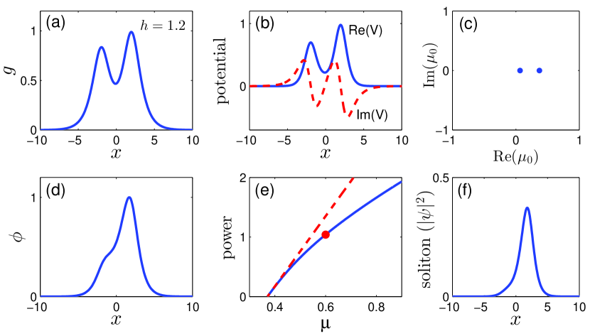
Figure 1: (a) The example function $g(x)$ in Eq. (90) with $h=1.2$; (b) Complex potential $V(x)$ for the $g(x)$ function in (a); (c) Eigenvalues $\mu_{0}$ of the eigenmode problem (32); (d) Eigenfunction $\phi$ of the largest eigenvalue in (c); (e) Power curve of solitons bifurcating from the linear mode in (d) under focusing nonlinearity [solid blue: numerical values; dashed red: the line with the theoretical slope value (91)]; (f) Soliton ($|\psi|^{2}$) at the marked point of the power curve.

As parameter $h$ in the $g(x)$ function (90) varies, the discrete eigenvalue $\mu_{0}$ will change [see Fig. 2(a)]. When $h$ drops below 0.926, $\mu_{0}$ will fall under 0.25, entering the $\sqrt{4\mu_{0}}<\beta$ regime (where Assumption 3 does not hold). In order to test our theory for both $\sqrt{4\mu_{0}}>\beta$ and $\sqrt{4\mu_{0}}<\beta$ cases, we have plotted in Fig. 2(b) the theoretical predictions for the power slope $P_{\rm anal}^{\prime}(\mu_{0})$ in Eq. (91) for $0.5\leq h\leq 1.5$, which encompasses both cases. The reader is reminded that the $c_{0}$ formula is given by Eq. (77) when $\sqrt{4\mu_{0}}>\beta$ and by Eq. (89) when $\sqrt{4\mu_{0}}<\beta$. In the same figure, numerically obtained power slopes $P^{\prime}(\mu_{0})$ for each $h$ value are shown as well. It is seen that numerical and analytical slope values exactly match each other, confirming the accuracy of our theoretical analysis in sections 4.3-4.4.

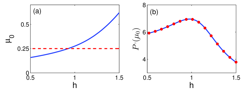
Figure 2: (a) Linear eigenvalue $\mu_{0}$ in Eq. (32) for the $g(x)$ function (90) at various $h$ values; the horizontal dashed line is at $\mu_{0}=1/4$; (b) comparison on the slope of the power curve at the bifurcation point $\mu_{0}$ between numerical values (solid blue) and analytical predictions (red dots).

Example 2  As for the second example, we consider the potential (5) with

$$g(x)=2e^{-x^{2}/4}+e^{-(x-3)^{2}}.$$ (92)

The resulting potential $V(x)$ is displayed in Fig. 3(a). The tails of this potential decay like a Guassian, which is faster than exponential. Thus the results in Sec. 4.4 apply. In this case, analytical expressions for the tail functions $\tau^{\pm}(x)$ of $\phi_{2}(x)$ in Eq. (83) are not easy to obtain, but numerical approximations can be readily computed. Specifically we select the $\phi_{2}(x)$ function by requiring that for $x\rightarrow-\infty$ the function decay like a gaussian and take this tail to be $\tau^{-}(x)$. Now for $x\rightarrow+\infty$, the dominant decay of this tail is exponential, i.e., the tail term $\tau^{+}(x)$ decays faster than $e^{-\sqrt{4\mu_{0}}x}$ in Eq. (83), thus one must first find the coefficient $\kappa_{2}$ of the exponential tail from large-$x$ values of $\phi_{2}(x)$. Then subtracting away this exponential tail from $\phi_{2}(x)$, the remaining tail is then $\tau^{+}(x)$. To obtain $\chi_{1}^{\pm}$ and $\chi_{2}^{\pm}$ in Eq. (87), we first compute $R_{11}(x)$ and $R_{12}(x)$ from the inhomogeneous equation (40), with $F$ replaced by $f_{1}$ and $f_{2}$, under the initial conditions (86). This is done by integrating the inhomogeneous equation from $x=0$ out to $x=\pm\infty$. By substracting their (slower-decaying) exponential tails and comparing the remaining tails with $\tau^{\pm}(x)$ in $\phi_{2}$, $\chi_{1}^{\pm}$ and $\chi_{2}^{\pm}$ can then be ascertained. From these numbers, the $c_{0}$ value is calculated from formula (89).

Now we compare these analytical predictions against numerical results. Solving the eigenvalue problem (32), we find three discrete real eigenvalues, the largest being $\mu_{0}\approx 2.6923$. From this eigenmode, we have confirmed that a soliton family indeed bifurcates out. If the nonlinearity is focusing ($\sigma=1$), the power curve of this soliton family is plotted in Fig. 3(b), and the profile of the soliton at the marked point of the power curve (with $\mu=3.5$) is illustrated in panel (c). On the power curve, the line with analytically predicted power slope at the bifurcation point from Eqs. (89) and (91) is also plotted. It is seen that this analytical power slope matches the numerical one very well.

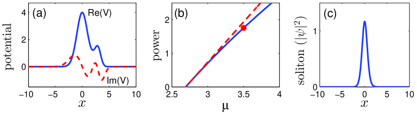
Figure 3: (a) Complex potential $V(x)$ for the $g(x)$ function in Example 2; (b) Power curve of solitons under focusing nonlinearity [solid blue: numerical values; dashed red: the line with the theoretical slope (91)]; (c) Soliton ($|\psi|^{2}$) at the marked point of the power curve.

5 Extension to more general nonlinearities

In this section, we show that the results in the previous sections can be readily extended to a wider class of nonlinearities

$$i\Psi_{t}+\Psi_{xx}+V(x)\Psi+G(|\Psi|^{2})\Psi=0,$$ (93)

where $G(\cdot)$ is an arbitrary real function, and $V(x)$ is a complex potential. Solitons (3) in this equation satisfy the stationary equation

$$\psi_{xx}-\mu\psi+V(x)\psi+G(|\psi|^{2})\psi=0.$$ (94)

Just as in the case of cubic nonlinearity, in the absence of the potential [$V(x)=0$], this soliton equation admits two constants of motion. Assuming that the constant of motion in the presence of the complex potential $V(x)$ is a continuous deformation of those without the potential, we can show by the same technique employed in Sec. 3 that the only complex potentials which admit a constant of motion are those in the special form of (5), and the corresponding constant of motion is

$$J=r_{x}^{2}-\mu r^{2}+H(r^{2})+r^{2}(\theta+g)^{2},$$ (95)

where $H(z)=\int G(z)dz$, and $dJ/dx=0$.

We can also show that for these general nonlinearities, with potentials of the form (5), continuous families of solitons still bifurcate out from linear discrete eigenmodes. Without loss of generality, we require $H(0)=0$. Then for solitons, $J=0$. Using this relation, the equation for the complex soliton $\psi(x)$ is reduced to the following second-order equation for the real amplitude variable $R(x)=|\psi(x)|^{2}$:

$$R_{xx}-4\mu R+2R\hskip 1.42271ptG(R)+2H(R)\pm 2g\sqrt{4\mu R^{2}-4R\hskip 1.42271ptH(R)-R_{x}^{2}}=0.$$ (96)

This equation is the analog of Eq. (28) for the cubic NLS equation (1). Repeating similar analysis as in the earlier text, these soliton bifurcations can be explicitly calculated.

To illustrate these analytical results for general nonlinearities, we consider the following example with a saturable nonlinearity.

Example 3  Consider the NLS equation (93) with a saturable nonlinearity and complex potential,

$$i\Psi_{t}+\Psi_{xx}+V(x)\Psi+\frac{|\Psi|^{2}}{1+|\Psi|^{2}}\Psi=0,$$ (97)

where the potential $V(x)$ is of the special form (5) with $g(x)$ chosen the same as in Example 1 [i.e., $g(x)$ is given by Eq. (90)], with $h$ fixed as $h=1.2$. Solitons in this equation are sought of the form (3), where $\psi(x)$ solves

$$\psi_{xx}-\mu\psi+V(x)\psi+\frac{|\psi|^{2}}{1+|\psi|^{2}}\psi=0.$$ (98)

Since the potential here is the same as that in Example 1, discrete eigenvalues in the linear equation (32) remain the same as those shown in Fig. 1(c), with the larger one being $\mu_{0}\approx 0.3708$. From this eigenmode, we have confirmed that a continuous family of solitons bifurcates out, whose power curve is displayed in Fig. 4(a). At the marked point of the power curve, the corresponding soliton is plotted in Fig. 4(b). This example verifies that the bifurcation of soliton families in complex potentials (5) occurs for a wider class of nonlinearities (93).

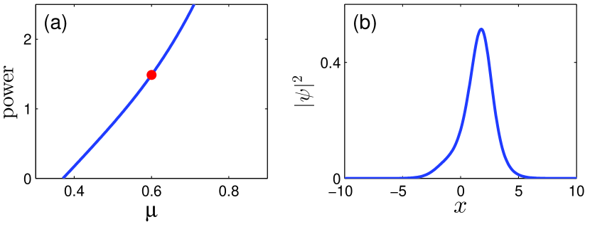
Figure 4: (a) Power curve of solitons bifurcating from a linear mode in Example 3; (b) Soliton ($|\psi|^{2}$) at the marked point of the power curve.

6 Summary and discussion

In this paper, we have analyzed soliton families in NLS-type equations with non-$\mathcal{PT}$-symmetric complex potentials. Under a weak assumption, we have shown that stationary forms of these equations admit a constant of motion if and only if the complex potential is of the special form (5). Using this constant of motion, we reduced the second-order complex soliton equation to a new second-order real equation for the amplitude of the soliton. From this new soliton equation, we showed, by perturbation methods, that continuous families of solitons always bifurcate out from linear eigenmodes for this special form of complex potentials. These results hold not only for the cubic nonlinearity, but also for a much wider class of nonlinearities. While it has been known that $\mathcal{PT}$-symmetric dissipative systems share some important properties with conservative systems, the results in this paper reveal that certain types of non-$\mathcal{PT}$-symmetric dissipative systems can also share such properties of conservative systems (such as the existence of soliton families).

Our results also shed light on a more general question: what non-$\mathcal{PT}$-symmetric complex potentials in the NLS-type equations (1) and (93) admit continuous families of solitons? In the absence of $\mathcal{PT}$symmetry, the existence of a constant of motion in the stationary soliton equation is critical for the existence of soliton families. We have shown that such a constant of motion exists only for special potentials of the form (5), assuming this constant of motion is a continuous deformation of that from the potential-free equation. Since this assumption is reasonable, we conjecture that the only non-$\mathcal{PT}$-symmetric complex potentials which admit soliton families are those of the special form (5).

It should be pointed out that the question of solitons in non-$\mathcal{PT}$-symmetric potentials is closely related to the question of non-$\mathcal{PT}$-symmetric solitons in $\mathcal{PT}$-symmetric potentials. Indeed, for $\mathcal{PT}$-symmetric potentials of the same special form (5), where $g(x)$ is taken to be even, it has been shown numerically that symmetry breaking of solitons can occur [28]. As a consequence, continuous families of non-$\mathcal{PT}$-symmetric solitons exist in a $\mathcal{PT}$-symmetric potential. This symmetry breaking is surprising since it is forbidden in generic $\mathcal{PT}$-symmetric potentials [29]. Analytical understanding of this symmetry breaking is still an open question, however, based on the analysis in this paper, it is hopeful that this symmetry breaking can now be analytically studied. But this lies outside the scope of the present article.

In the end, we mention that bifurcation of soliton families from linear modes occurs in special forms of two-dimensional non-$\mathcal{PT}$-symmetric complex potentials as well [30]. Analytical understanding of such bifurcations in two spatial dimensions is a more challenging question which merits further investigation.

References

- [1] O
- [2] C.M. Bender & S. Boettcher, Real spectra in non-Hermitian Hamiltonians having PT symmetry, Phys. Rev. Lett. 80, 5243–5246 (1998).
- [3] Z.H. Musslimani, K.G. Makris, R. El-Ganainy & D.N. Christodoulides, Optical solitons in PT periodic potentials, Phys. Rev. Lett. 100, 030402 (2008).
- [4] H. Wang & J. Wang, Defect solitons in parity-time periodic potentials. Opt. Exp. 19, 4030–4035 (2011).
- [5] Z. Lu & Z. Zhang, Defect solitons in parity-time symmetric superlattices, Opt. Exp. 19, 11457–11462 (2011).
- [6] F. K. Abdullaev, Y. V. Kartashov, V. V. Konotop & D. A. Zezyulin, Solitons in PT-symmetric nonlinear lattices. Phys. Rev. A 83, 041805 (2011).
- [7] Y. He, X. Zhu, D. Mihalache, J. Liu & Z. Chen, Lattice solitons in PT-symmetric mixed linear-nonlinear optical lattices, Phys. Rev. A 85, 013831 (2012).
- [8] S. Nixon, L. Ge & J. Yang, Stability analysis for solitons in PT-symmetric optical lattices, Phys. Rev. A 85, 023822 (2012).
- [9] D. A. Zezyulin & V.V. Konotop, Nonlinear modes in the harmonic PT-symmetric potential, Phys. Rev. A 85, 043840 (2012).
- [10] C. Huang, C. Li, & L. Dong, Stabilization of multipole-mode solitons in mixed linear-nonlinear lattices with a PT symmetry, Opt. Exp. 21, 3917–3925 (2013).
- [11] Y.V. Kartashov, Vector solitons in parity-time-symmetric lattices, Opt. Lett. 38, 2600–2603 (2013).
- [12] R. Driben & B. A. Malomed, Stability of solitons in parity-time-symmetric couplers, Opt. Lett. 36, 4323–4325 (2011).
- [13] N. V. Alexeeva, I. V. Barashenkov, A. A. Sukhorukov & Yu. S. Kivshar, Optical solitons in PT-symmetric nonlinear couplers with gain and loss, Phys. Rev. A 85, 063837 (2012).
- [14] F. C. Moreira, F. Kh. Abdullaev, V. V. Konotop & A. V. Yulin, Localized modes in media with PT-symmetric localized potential, Phys. Rev. A 86, 053815 (2012).
- [15] V. V. Konotop, D. E. Pelinovsky & D. A. Zezyulin, Discrete solitons in PT-symmetric lattices, Euro. Phys. Lett. 100, 56006 (2012).
- [16] P. G. Kevrekidis, D. E. Pelinovsky & D. Y. Tyugin, Nonlinear stationary states in PT-symmetric lattices, SIAM J. Appl. Dyn. Syst., 12, 1210–1236 (2013).
- [17] K. Li & P. G. Kevrekidis, PT-symmetric oligomers: Analytical solutions, linear stability, and nonlinear dynamics, Phys. Rev. E 83, 066608 (2011).
- [18] D. A. Zezyulin & V.V. Konotop, Nonlinear Modes in Finite-Dimensional PT-Symmetric Systems, Phys. Rev. Lett. 108, 213906 (2012).
- [19] D. A. Zezyulin & V.V. Konotop, Stationary modes and integrals of motion in nonlinear lattices with PT -symmetric linear part, J. Phys. A 46, 415301 (2013).
- [20] M. Wimmer, A. Regensburger, M.A. Miri, C. Bersch, D.N. Christodoulides & U. Peschel, Observation of optical solitons in -symmetric lattices, Nature Communications 6:7782 (2015).
- [21] J. Yang, Necessity of PT symmetry for soliton families in one-dimensional complex potentials, Phys. Lett. A 378, 367–373 (2014).
- [22] E.N. Tsoy, I.M. Allayarov & F. Kh. Abdullaev, Stable localized modes in asymmetric waveguides with gain and loss, Opt. Lett. 39, 4215–4218 (2014).
- [23] V. V. Konotop & D. A. Zezyulin, Families of stationary modes in complex potentials, Opt. Lett. 39, 5535–5538 (2014).
- [24] J. Yang, Nonlinear Waves in Integrable and Nonintegrable Systems (SIAM, Philadelphia, 2010).
- [25] L.P. Pitaevskii & S. Stringari, Bose- Einstein Condensation (Oxford University Press, Oxford, 2003).
- [26] S. Klaiman, U. Günther & N. Moiseyev, Visualization of Branch Points in PT-Symmetric Waveguides, Phys. Rev. Lett. 101, 080402 (2008).
- [27] W. Hereman, Symbolic computation of conservation laws of nonlinear partial differential equations in multi-dimensions, International J. Quantum Chemistry 106, 278–299 (2006).
- [28] J. Yang, Symmetry breaking of solitons in one-dimensional parity-time-symmetric optical potentials, Opt. Lett. 39, 5547-5550 (2014).
- [29] J. Yang, Can parity-time-symmetric potentials support families of non-parity-time-symmetric solitons? Stud. Appl. Math. 132, 332–353 (2014).
- [30] J. Yang, Symmetry breaking of solitons in two-dimensional complex potentials, Phys. Rev. E 91, 023201 (2015).