Analytic potentials and vibrational energies for Li₂ states dissociating to $\mbox{Li}\left(2S\right)+\mbox{Li}\left(3P\right)$. Part 1: The ${}^{2S+1}\Pi_{\nicefrac{{u}}{{g}}}$ states

Abstract

Analytic potentials are built for all four ${}^{2S+1}\Pi_{u/g}$ states of Li₂ dissociating to Li$(2S)$ + Li$(3P)$: $3b(3^{3}\Pi_{u})$, $3B(3^{1}\Pi_{u})$, $3C(3^{1}\Pi_{g}),$ and $3d(3^{3}\Pi_{g})$. These potentials include the effect of spin-orbit coupling for large internuclear distances, and include state of the art long-range constants. This is the first successful demonstration of fully analytic diatomic potentials that capture features that are usually considered too difficult to capture without a point-wise potential, such as multiple minima, and shelves. Vibrational energies for each potential are presented for the isotopologues ^6,6Li₂, ^6,7Li₂, ^7,7Li₂, and the elusive ‘halo nucleonic molecule’ ^11,11Li₂. These energies are claimed to be accurate enough for new high-precision experimental setups such as the one presented in [Sebastian et al. Phys. Rev. A, 90, 033417 (2014)] to measure and assign energy levels of these electronic states, all of which have not yet been explored in the long-range region. Measuring energies in the long-range region of these electronic states may be significant for studying the ab initio vs experiment discrepancy discussed in [Tang et al. Phys. Rev. A, 84, 052502 (2014)] for the $C_{3}$ long-range constant of Lithium, which has significance for improving the SI definition of the second.

Very little is known about the Li₂ electronic states dissociating to the $2S+3P$ asymptote. Out of the first 5 asymptotes (from lowest to highest: $2S+2S$, $2S+2P$, $2S+3S$, $2P+2P$ and $2S+3P$), the $2S+3P$ is the only one for which an empirical dissociation energy has not been determined for any of the electronic states dissociating to it. Furthermore, the only measurements that have been made for electronic states dissociating to $2S+3P$, were for the $3c(3^{3}\Sigma_{g}^{+})$ state Xie and Field (1986a); Yiannopoulou et al. (1995a); Li et al. (2007) the $6X(6^{1}\Sigma_{g}^{+})$ state Bernheim et al. (1983); Song et al. (2002), and the $3d(3^{3}\Pi_{g})$ state Yiannopoulou et al. (1995b); Li et al. (1996a, b); Ivanov et al. (1999). No measurements have been done on the other states dissociating to $2S+3P$.

Very recently, a promising experiment has been setup with the ability to use photoassociation in a magneto-optical trap to make ultra-cold ⁶Li₂ molecules dissociating to the $2S+3P$ asymptote Sebastian et al. (2014), much like slightly earlier experiments which have already been successful for creating ultra-cold ⁶Li₂ molecules dissociating to $2S+2P$ with very similar techniques Semczuk et al. (2013); Gunton et al. (2013). Measurements of the binding energies for levels very close to the $2S+3P$ asymptote would allow for an empirical determination of the long-range constant $C_{3}^{2S+3P}$ which is the leading interaction constant in the potential energy between Li$(2S)$ and Li$(3P)$.

$u^{3b}(r)$	=	$\begin{cases}\\ \\ \\ \\ \end{cases}$	$u^{3b,0_{u}^{+}}(r)$	$\xrightarrow{\qquad u^{6A,0_{u}^{+}}(r)\qquad}$	$2S_{1/2}+3P_{1/2}$	(higher)
			$u^{3b,0_{u}^{-}}(r)$	$\xrightarrow{\qquad u^{6a,0_{u}^{-}}(r)\qquad}$	$2S_{1/2}+3P_{3/2}$	(lower)
			$u^{3b,1_{u}}(r)$	$\xrightarrow{\,\,u^{3B,1_{u}}(r),u^{6a,1_{u}}(r)\,\,}$	$2S_{1/2}+3P_{3/2}$	(lowest)
			$u^{3b,2_{u}}(r)$	$\xrightarrow{\qquad\qquad\qquad\qquad}$	$2S_{1/2}+3P_{3/2}$
$u^{3B}(r)$	=		$u^{3B,1_{u}}(r)$	$\xrightarrow{\,\,u^{6a,1_{u}}(r),u^{3b,1_{u}}(r)\,\,}$	$2S_{1/2}+3P_{3/2}$	(middle)
$u^{3C}(r)$	=		$u^{3C,1_{g}}(r)$	$\xrightarrow{\,\,u^{3c,1_{g}}(r),u^{3d,1_{g}}(r)\,\,}$	$2S_{1/2}+3P_{3/2}$	(middle)
$u^{3d}(r)$	=	$\begin{cases}\\ \\ \\ \\ \end{cases}$	$u^{3d,0_{g}^{+}}(r)$	$\xrightarrow{\qquad u^{6X,0_{g}^{+}}(r)\qquad}$	$2S_{1/2}+3P_{1/2}$	(lower)
			$u^{3d,0_{g}^{-}}(r)$	$\xrightarrow{\qquad u^{3c,0_{g}^{-}}(r)\qquad}$	$2S_{1/2}+3P_{3/2}$	(higher)
			$u^{3d,1_{g}}(r)$	$\xrightarrow{\,\,u^{3c,1_{g}}(r),u^{3C,1_{g}}(r)\,\,}$	$2S_{1/2}+3P_{3/2}$	(highest)
			$u^{3d,2_{g}}(r)$	$\xrightarrow{\qquad\qquad\qquad\qquad}$	$2S_{1/2}+3P_{3/2}$

At the lower asymptote of $2S+2P$, there is a discrepancy between experiment and theory for the long-range constant $C_{3}^{2S+3P}$, despite Li only having 3e^- and the experimental value being the most precisely determined oscillator strength ever determined for a molecule, by an order of magnitude Tang et al. (2011). This has various consequences, reaching as far as limiting progress towards improving the precision of the SI definition of the second Mitroy et al. (2010). More precise atomic clocks are needed for various applications. The current definition of the second is based on a clock transition frequency in Cs with a relative uncertainty of $\sim 5\times 10^{-16}$, and a commonly quoted target for improved precision is $10^{-18}$ Mitroy et al. (2010). The largest source of uncertainty limiting atomic clock precision is the blackbody radiation shift, which depends on the static dipole polarizability of the system being used for the atomic clock Mitroy et al. (2010). Lithium is expected to play a major role in polarizability metrology, since polarizability ratios can be measured much more precisely than individual polarizabilities Cronin et al. (2009) and Li is the preferred choice for the standard in the denominator of such a ratio Mitroy et al. (2010). The discrepancy in $C_{3}$ limits the accuracy of a potential Li-based standard for polarizabilities Tang et al. (2011), and hence indirectly impacts progress towards improving the SI definition of the second.

Regarding the empirical value for $C_{3}^{2S+2P}$, for most electronic states, the mixing of various states towards the $2S+2P$ asymptote significantly complicates the expressions from which $C_{3}$ is fitted Dattani and LeRoy (2015); Dattani and Le Roy (2011); Le Roy et al. (2009); Aubert-Frécon et al. (1998); Bussery and Aubert-Frecon (1985). The complicated expressions for this mixing are the same at the $2S+3P$ asymptote as they are for the $2S+2P$ asymptote Aubert-Frécon (2015), but the fine structure splitting parameter which governs the significance of this mixing, is about 3.5 times smaller at the $2S+3P$ asymptote than at the $2S+2P$ asymptote. For $2S+2P$ the fine structure splitting parameter for ⁶Li is $\Delta E_{2^{2}P_{\nicefrac{{3}}{{2}}}\leftarrow 2^{2}P_{\nicefrac{{1}}{{2}}}}=D_{2}-D_{1}=0.335\,324\,6$ cm^-1 Semczuk et al. (2013); Gunton et al. (2013); Brown et al. (2013); Sansonetti et al. (2011), while for $2S+3P$ it is only $\Delta E_{3^{2}P_{\nicefrac{{3}}{{2}}}\leftarrow 3^{2}P_{\nicefrac{{1}}{{2}}}}=0.096$ cm^-1 Sansonetti et al. (1995). Therefore, $C_{3}^{2S+3P}$ might be a better benchmark for an ab initio vs experiment comparison than $C_{3}^{2S+2P}$, as the effect of this complication is smaller.

Measuring and assigning molecular energy levels using photoassociation requires reasonably accurate predictions which come from eigenvalues of a Schrödinger equation, and hence require a reasonably accurate potential energy surface. Due to the shortage of measurements on the Li₂ ${}^{2S+1}\Pi_{\nicefrac{{u}}{{g}}}$ states dissociating to $2S+3P$, the most accurate potentials come from purely ab initio calculations. For the $3c(3^{3}\Sigma_{g}^{+})$ and $3A(3^{1}\Sigma_{u}^{+})$ states, ab initio calculations were reported in 1985 Schmidt-Mink et al. (1985), 1995 Poteau and Spiegelmann (1995), 2006 Jasik and Sienkiewicz (2006) and 2014 Musial and Kucharski (2014); Lee (2014); and for the $3d(3^{3}\Pi_{g})$ state in 1995 Yiannopoulou et al. (1995b) and 2014 Musial and Kucharski (2014); Lee (2014). But for the rest of the states dissociating to $2S+3P$; namely $3b(3^{3}\Pi_{u})$, $6X(6^{1}\Sigma_{g}^{+})$, $3B(3^{1}\Pi_{u})$, $3C(3^{1}\Pi_{g})$, and $6a(6^{3}\Sigma_{u}^{+})$; the only ab initio calculations reported were in Poteau and Spiegelmann (1995); Musial and Kucharski (2014); Lee (2014). All of these ab initio papers also reported potentials for states dissociating to lower asymptotes, where plenty of experimental data is available to gauge the quality of the calculations.

In my very recent paper on comparing experiment to ab initio for the $b(1^{3}\Pi_{u})$ state Dattani and LeRoy (2015), it was found that the ab initio potential of Musial and Kucharski (2014) predicted all vibrational binding energies with a disagreement of $<12$ cm^-1 with the corresponding energies of the empirical potential. Furthermore there was always $<0.8$ cm^-1 disagreement between the empirical and ab initio vibrational energy spacings. Finally, when comparing the dissociation energies $\mathfrak{\mathfrak{D}}_{e}$ from Musial and Kucharski (2014) to the corresponding experimental values for all states which have empirical $\mathfrak{D}_{e}$ values available, the ab initio values from Musial and Kucharski (2014) were never in disagreement by more than 68 cm^-1. Therefore, the ab initio potentials from Musial and Kucharski (2014) for the states dissociating to $2S+3P$ are expected to be a good starting point for predicting energy levels with the precision required for photoassociation experiments as in Semczuk et al. (2013); Gunton et al. (2013) and as may be preformed with the new setup in Sebastian et al. (2014) which is capable of detecting states dissociating to $2S+3P$.

However, the ab initio calculations of Musial and Kucharski (2014) still have some major drawbacks (including, but not limited to):

1. the ab initio points are not on a dense enough mesh to use as the mesh for solving the effective radial Schrödinger equation for predicting the vibrational energies (especially for large distances where the energies become more important for fitting an empirical $C_{3}$ value, and for experiments such as those potentially resulting from a setup such as in Sebastian et al. (2014));

2. the ab initio points neglect the effect of spin-orbit coupling, which is particularly important for $nS+n^{\prime}P$ states of Li₂, where the effect of interstate coupling has been shown to be absolutely obligatory for describing the high vibrational energy measurements Le Roy et al. (2009); Dattani and Le Roy (2011); Semczuk et al. (2013); Gunton et al. (2013);

3. the ab initio points do not go beyond the Born-Oppenheimer approximation (so do not distinguish between different isotopologues such as ^6,6Li${}_{2},$ ^6,7Li₂, ^7,7Li₂, and the elusive ‘halo nucleonic’ isotopologues containing ¹¹Li), and they are non-relativistic.

Drawback (1) is usually treated by fitting an interpolant through the ab initio points, but the resulting energies predicted after solving the Schrödinger equation, will be very sensitive to the type of interpolant used, especially at the level of precision of photoassociation experiments (the precision in the Li₂ measurements of Semczuk et al. (2013); Gunton et al. (2013) was $\pm 0.00002$ cm^-1 or $\pm 600$ kHz). Also, if for sake of ease, a spline interpolant is used, it would be defined piecewise and would have discontinuous first derivatives. The spline also knows nothing about the physics of nature, and will therefore not know what to do in regions where fewer ab initio points are available (in this example, for large internuclear distances).

Rather than interpolating with a spline, we can fit to a fully analytic model potential that has the correct theoretical behavior incorporated in the long-range region where fewer ab initio points are available, and this addresses drawback (2) as well, since the effect of spin-orbit coupling at long-range can easily be incorporated into the model. Part of drawback (3) can also be addressed by fitting to a model potential, because the model can also build in some types of relativistic effects such as QED retardation, as was attempted in Le Roy et al. (2009); Dattani and Le Roy (2011); Semczuk et al. (2013); Gunton et al. (2013). In 2011 the Morse/long-range (MLR) potential was fitted to spectroscopic data for the $c(1^{3}\Sigma_{g}^{+})$ state of Li₂ where there was a gap of $>5000$ cm^-1 between data near the bottom of the potential’s well, and data at the very top Dattani and Le Roy (2011). In 2013 it was found by experiment that vibrational energies predicted from this MLR potential in the very middle of this gap were correct to about 1 cm^-1 Semczuk et al. (2013). Therefore, fitting the ab initio data to the MLR model can provide reliable energy predictions in regions where ab initio points are lacking or are poor in quality.

Therefore, in this paper MLR models that incorporate the long-range theoretical effect of spin-orbit coupling are fitted to the ab initio points from Musial and Kucharski (2014) for the ${}^{2S+1}\Pi_{\nicefrac{{u}}{{g}}}$ states of Li₂ dissociating to $2S+3P$. Drawback (3) is not addressed in this paper. However, Born-Oppenheimer breakdown (BOB) corrections could have been added to the ab initio points using the molecular electron wavefunction as described in Dattani and LeRoy (2015). Alternatively, the entire ab initio calculation can be redone using a non-Born-Oppenheimer approach as has been done for up to 6e^- Bubin et al. (2009), but the a posteriori approach of doing a Born-Oppenheimer calculation and then adding BOB corrections afterwards has been shown to work better according to the agreement between experiment and theory for BeH Dattani (2015); Bubin and Adamowicz (2007). Also, DKH (Douglas-Kroll-Hess) relativistic corrections can be added to the ab initio potential as in Koput (2011), and QED effects can also be added as was done for H₂ in Komasa et al. (2011) and HeH⁺ in Pachucki and Komasa (2012). If any of these answers to drawback (3) were to be addressed by adding corrections to the ab initio points of Musial and Kucharski (2014), the procedure applied in the present paper for fitting an MLR function to ab initio points, could be repeated for even more accurate analytic potentials.

I Extending the ab initio calculations

The ab initio calculations in Musial and Kucharski (2014) did not go beyond 22 Å. However, beyond a certain length, analytic expressions for the potential can be derived from the theory of atom-atom interactions with disregard for the effect of overlap between each atom’s electronic wavefunction. These analytic expressions are based on long-range constants that come from atomic ab initio calculations rather than molecular ones, so for Li₂ the calculations only involve 3e^- rather than 6e^-. This means, for example, that a coupled cluster calculation taking account of the full configuration interaction (FCI) of a basis set only needs to go up to triple excitations (CCSDT, whose scaling with respect to the number of basis functions $N$ is $\sim N^{8}$ and has been implemented since 1987 Noga and Bartlett (1987)); whereas a molecular calculation on Li₂ would require all the way up to hexuple excitations (CCSDTQPH, which scales as $\sim N^{14}$, and has been implemented in only very few studies since 2000 Hirata and Bartlett (2000); Kallay and Surjan (2001); Kallay and Gauss (2004); Evangelista et al. (2006); DeYonker and Allen (2012); DeYonker and Shah (2014) with basis sets that have not yet gone beyond the cc-pVDZ-DK basis set DeYonker and Shah (2014)). Furthermore, 3e^- is the limit at which the integrals have been expressed analytically for explicitly correlated Slater wavefunctions, so treating 6e^- would either require numerically calculating the integrals (which would be too slow even for small basis sets), or explicitly correlated Gaussian wavefunctions (which do not necessarily have the correct short- and long-range behavior). Therefore, beyond a certain distance the analytic expressions ignoring wavefunction overlap but using long-range constants for Li based on 3e^- ab initio calculations, are expected to be more accurate than the 6e^- ab initio calculations of Musial and Kucharski (2014) that include wavefunction overlap. The distance at which this trade-off begins to lean in favor of the analytic expressions is heuristically given by the Le Roy radius LeRoy (1973, 1974); Ji et al. (1995).

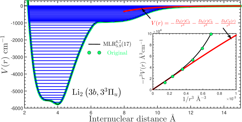
Figure 1: Point-wise original, and analytic MLR potentials for $3b(3^{3}\Pi_{u})$ representing the ab initio calculations of Musial and Kucharski (2014). The inset shows the long-range behavior in Le Roy space: it demonstrates that the original ab initio points unphysically dip below the theoretical curve, while the MLR behaves correctly.

Another advantage of using the analytic expressions, is that the ab initio calculations of Musial and Kucharski (2014) do not include the effect of spin-orbit coupling, but for alkali atoms dissociating to $nS+n^{\prime}P$ asymptotes, the effect of spin-orbit coupling at long-range has been determined analytically Bussery and Aubert-Frecon (1985); Aubert-Frécon et al. (1998). Although all papers discussing these analytic expressions to date only mention $nS+nP$ asymptotes, the expressions are also the same for $nS+n^{\prime}P$ asymptotes when $n\neq n^{\prime}$ Aubert-Frécon (2015).

I.1 Le Roy radii

The $m$-dependent Le Roy radius is given by Ji et al. Ji et al. (1995):

$$R_{{\rm LR}-m}\equiv 2\sqrt{3}\left(\langle nlm|z^{2}|nlm\rangle^{\nicefrac{{1}}{{2}}}+\langle n^{\prime}l^{\prime}m^{\prime}|z^{2}|n^{\prime}l^{\prime}m^{\prime}\rangle^{\nicefrac{{1}}{{2}}}\right),$$ (1)

where for hydrogen-like atoms we have Ji et al. (1995):

$$\langle nlm|z^{2}|nlm\rangle^{\nicefrac{{1}}{{2}}}=\left(\frac{1}{3}-\frac{2}{3}\frac{3m^{2}-l(l+1)}{(2l+3)(2l-1)}\right)^{\nicefrac{{1}}{{2}}}\langle nl|r^{2}|nl\rangle^{\nicefrac{{1}}{{2}}}$$ (2)

and for $l=0$ we have (because $m$ is also $0$) Ji et al. (1995):

$$\langle nlm|z^{2}|nlm\rangle^{\nicefrac{{1}}{{2}}}=\frac{1}{\sqrt{3}}\langle r^{2}\rangle^{\nicefrac{{1}}{{2}}}.$$ (3)

This means that if both atoms of a diatomic molecule are in $S$ states, the fact that $l=l^{\prime}=0$ reduces Eq. 1 to the original Le Roy radius of LeRoy (1973, 1974):

$$r_{{\rm LR}} \equiv 2\left(\langle r_{{\rm A}}^{2}\rangle^{\nicefrac{{1}}{{2}}}+\langle r_{{\rm B}}^{2}\rangle^{\nicefrac{{1}}{{2}}}\right).$$ (4)

However for a hydrogenic atom with $l\neq 0$ we have Ji et al. (1995):

$$\langle nl|r^{2}|nl\rangle^{\nicefrac{{1}}{{2}}}=a_{\mu}\frac{n^{2}}{Z}\left(1+\frac{3}{2}\left(1-\frac{l(l+1)-\nicefrac{{1}}{{3}}}{n^{2}}\right)\right)^{\nicefrac{{1}}{{2}}},$$ (5)

where $Z$ is the effective nuclear charge, $a_{\mu}=a_{0}\frac{m_{N}}{\mu}$ is the Bohr radius scaled by the ratio of the mass of the nucleus $m_{N}$ to the reduced mass $\mu$ of the atom. And for alkali atoms, the principal quantum number $n$ is replaced by $n-\alpha(l)$, where $\alpha(l)$ is the quantum defect and can be found in standard references such as Ref [29] of Ji et al. (1995). Using $\alpha(p)=1.59$ for Li, assuming that $\mu_{{}^{6}{\rm Li}}=\frac{m_{e}M_{{}^{6}{\rm Li}}}{m_{e}+M_{{}^{6}{\rm Li}}}\approx m_{e}=1\,\mbox{a.u.}$, and using $\langle r^{2}\rangle$ values calculated in Zhang et al. (2007), we are able to calculate Eq. 1 for Li₂ molecules dissociating to various asymptotes, and we present these in Table 1.

Table 1: $m$-dependent Le Roy radii for Li₂ electronic states that approach $2s+ml$ in Hartree atomic units and spectroscopic units, and the constituent quantities that are used to calculate these radii.

	$\langle r^{2}\rangle$		$\langle nlm|z^{2}|nlm\rangle^{\nicefrac{{1}}{{2}}}$		$r_{{\rm LR-m}}(2s+ml)$		$r_{{\rm LR-m}}(2s+ml)$
	a.	u.	a.	u.	a.	u.	Å
$2s$	17.	47 Zhang et al. (2007)	17.	47 Zhang et al. (2007)	16.	7189	8.	8473
$2p$	27.	06 Zhang et al. (2007)	0.	3810	27.	0	14.	0
$3p$	168.	69 Zhang et al. (2007)	0.	5910	40.	0	20.	1

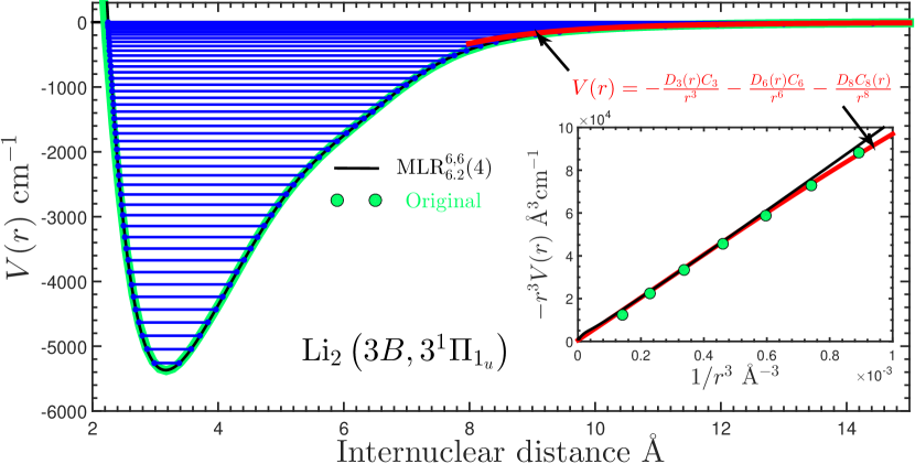
Figure 2: Point-wise original, and analytic MLR potentials for $3B(3^{1}\Pi_{1_{u}})$ representing the ab initio calculations of Musial and Kucharski (2014). The inset shows the long-range behavior in Le Roy space.

I.2 Long-range theory

It is well-known that for large internuclear distances, the MLR model becomes, Dattani and Le Roy (2011):

$$V(r)\simeq\mathfrak{D}_{e}-u(r)+\cdots.$$ (6)

Therefore, we can define $u(r)$ to be the analytic expression describing the theoretical interaction between the constituent atoms of the molecule. Each ${}^{2S+1}\Pi_{u/g}$ state considered in this paper has $\Omega_{u/g}$ daughter states resulting from the spin-orbit coupling that lifts the degeneracy. For the $2_{u}$ and $2_{g}$ states, which are daughters of $3b(3^{3}\Pi_{g})$ and $3d(3^{3}\Pi_{g})$ respectively, no other $\Omega=2$ state with the same $u/g$ symmetry approaches the $2S+3P$ asymptote, so the potential energy curves at long-range are not strongly influenced by other electronic states. Therefore, these states have the simplest form for $u(r)$:

$$u^{2_{\nicefrac{{u}}{{g}}}}(r) = -\left(\Delta E-\sum_{\begin{subarray}{c}m=3,6,8,\\ 9,10,11,\ldots\end{subarray}}\frac{C_{m}^{\left({}^{3}\Pi_{\nicefrac{{u}}{{g}}}\right)}}{r^{m}}\right)$$ (7)

$$= -\left(\Delta E-\frac{C_{3}^{\left({}^{3}\Pi_{\nicefrac{{u}}{{g}}}\right)}}{r^{3}}-\frac{C_{6}^{\left({}^{3}\Pi_{\nicefrac{{u}}{{g}}}\right)}}{r^{6}}-\frac{C_{8}^{\left({}^{3}\Pi_{\nicefrac{{u}}{{g}}}\right)}}{r^{8}}-\frac{C_{9}^{\left({}^{3}\Pi_{\nicefrac{{u}}{{g}}}\right)}}{r^{9}}-\frac{C_{10}^{\left({}^{3}\Pi_{\nicefrac{{u}}{{g}}}\right)}}{r^{10}}-\frac{C_{11}^{\left({}^{3}\Pi_{\nicefrac{{u}}{{g}}}\right)}}{r^{11}}\cdots\right),$$ (8)

where the zero of energy is the Li$(2S_{\nicefrac{{1}}{{2}}})$ + Li($3P_{\nicefrac{{1}}{{2}}}$) asymptote, and $\Delta E\equiv\Delta E_{3^{2}P_{3/2}\leftarrow 3^{2}P_{1/2}}$ is included since the $2_{u}$ and $2_{g}$ states both dissociate to Li$(2S_{\nicefrac{{1}}{{2}}})$ + Li($3P_{\nicefrac{{3}}{{2}}}$). The $3b(3^{3}\Pi_{u})$ state additionally has a daughter state of $1_{u}$ symmetry, along with $3B(3^{1}\Pi_{u})$; and the $3d(3^{3}\Pi_{g})$ state additionally has a daughter state of $1_{g}$ symmetry, along with $3C(3^{1}\Pi_{g})$. Since all $1_{\nicefrac{{u}}{{g}}}$ states approaching $2S+3P$ have two other $1_{u/g}$ states of the same $\nicefrac{{u}}{{g}}$ symmetry approaching $2S+3P$, the $u(r)$ for these states is defined as the highest, middle, or lowest energy eigenvalue of the following $3\times 3$ matrix (including the prefactor of $-1$) depending on whether the state in question is the lowest, middle, or highest in energy respectively:

$$\mathbf{u}^{1_{\nicefrac{{u}}{{g}}}}(r)=$$ (9)

$$-\left(\begin{array}[]{ccc}\frac{1}{3}{\displaystyle\sum_{m}\frac{C_{m}^{\left({}^{\nicefrac{{3}}{{1}}}\Sigma_{\nicefrac{{u}}{{g}}}^{+}\right)}+C_{m}^{\left({}^{\nicefrac{{1}}{{3}}}\Pi_{\nicefrac{{u}}{{g}}}\right)}+C_{m}^{\left({}^{\nicefrac{{3}}{{1}}}\Pi_{\nicefrac{{u}}{{g}}}\right)}}{r^{m}}}&\frac{1}{3\sqrt{2}}{\displaystyle\sum_{m}\frac{-2C_{m}^{\left({}^{\nicefrac{{3}}{{1}}}\Sigma_{\nicefrac{{u}}{{g}}}^{+}\right)}+C_{m}^{\left({}^{\nicefrac{{1}}{{3}}}\Pi_{\nicefrac{{u}}{{g}}}\right)}+C_{m}^{\left({}^{\nicefrac{{3}}{{1}}}\Pi_{\nicefrac{{u}}{{g}}}\right)}}{r^{m}}}&\frac{1}{\sqrt{6}}{\displaystyle\sum_{m}\frac{-C_{m}^{\left({}^{\nicefrac{{1}}{{3}}}\Pi_{\nicefrac{{u}}{{g}}}\right)}+C_{m}^{\left({}^{\nicefrac{{3}}{{1}}}\Pi_{\nicefrac{{u}}{{g}}}\right)}}{r^{m}}}\\ \frac{1}{3\sqrt{2}}{\displaystyle\sum_{m}\frac{-2C_{m}^{\left({}^{\nicefrac{{3}}{{1}}}\Sigma_{\nicefrac{{u}}{{g}}}^{+}\right)}+C_{m}^{\left({}^{\nicefrac{{1}}{{3}}}\Pi_{\nicefrac{{u}}{{g}}}\right)}+C_{m}^{\left({}^{\nicefrac{{3}}{{1}}}\Pi_{\nicefrac{{u}}{{g}}}\right)}}{r^{m}}}&\Delta E+\frac{1}{6}{\displaystyle\sum_{m}\frac{4C_{m}^{\left({}^{\nicefrac{{3}}{{1}}}\Sigma_{\nicefrac{{u}}{{g}}}^{+}\right)}+C_{m}^{\left({}^{\nicefrac{{1}}{{3}}}\Pi_{\nicefrac{{u}}{{g}}}\right)}+C_{m}^{\left({}^{\nicefrac{{3}}{{1}}}\Pi_{\nicefrac{{u}}{{g}}}\right)}}{r^{m}}}&\frac{1}{2\sqrt{3}}{\displaystyle\sum_{m}\frac{-C_{m}^{\left({}^{\nicefrac{{1}}{{3}}}\Pi_{\nicefrac{{u}}{{g}}}\right)}+C_{m}^{\left({}^{\nicefrac{{3}}{{1}}}\Pi_{\nicefrac{{u}}{{g}}}\right)}}{r^{m}}}\\ \frac{1}{\sqrt{6}}{\displaystyle\sum_{m}\frac{-C_{m}^{\left({}^{\nicefrac{{1}}{{3}}}\Pi_{\nicefrac{{u}}{{g}}}\right)}+C_{m}^{\left({}^{\nicefrac{{3}}{{1}}}\Pi_{\nicefrac{{u}}{{g}}}\right)}}{r^{m}}}&\frac{1}{2\sqrt{3}}{\displaystyle\sum_{m}\frac{-C_{m}^{\left({}^{\nicefrac{{1}}{{3}}}\Pi_{\nicefrac{{u}}{{g}}}\right)}+C_{m}^{\left({}^{\nicefrac{{3}}{{1}}}\Pi_{\nicefrac{{u}}{{g}}}\right)}}{r^{m}}}&-\Delta E+\frac{1}{2}{\displaystyle\sum_{m}\frac{C_{m}^{\left({}^{\nicefrac{{1}}{{3}}}\Pi_{\nicefrac{{u}}{{g}}}\right)}+C_{m}^{\left({}^{\nicefrac{{3}}{{1}}}\Pi_{\nicefrac{{u}}{{g}}}\right)}}{r^{m}}}\end{array}\right).$$ (10)

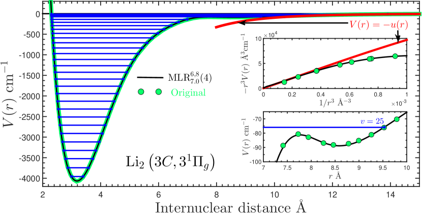
Figure 3: Point-wise original, and analytic MLR potentials for $3C(3^{1}\Pi_{g})$ representing the ab initio calculations of Musial and Kucharski (2014). The top inset shows the long-range behavior in Le Roy space, and the bottom inset shows that the MLR successfully captures the tiny second minimum which has a depth of $\approx 8.5$ cm^-1.

The notation ${}^{\nicefrac{{1}}{{3}}}\Lambda_{u/g}$ means $(^{1}\Lambda_{u}$ or ${}^{3}\Lambda_{g})$. The zero of energy is once again the Li$(2S_{\nicefrac{{1}}{{2}}})$ + Li($3P_{\nicefrac{{1}}{{2}}}$) asymptote. Finally, the $3b$ state additionally has $0_{u}^{+}$ and $0_{u}^{-}$ daughter states, and the $3d$ state additionally has $0_{g}^{+}$ and $0_{g}^{-}$ daughter states. Since all $0_{\nicefrac{{u}}{{g}}}^{\nicefrac{{+}}{{-}}}$ states approaching $2S+3P$ have one other $0_{\nicefrac{{u}}{{g}}}^{\nicefrac{{+}}{{-}}}$ state of the same $\nicefrac{{u}}{{g}}$ symmetry and the same $\nicefrac{{+}}{{-}}$ symmetry approaching $2S+3P$, the $u(r)$ for these states is defined as the higher, or lower energy eigenvalue of the following $2\times 2$ matrix (including the prefactor of $-1$) depending on whether the state in question is lower, or higher in energy respectively:

$$\mathbf{u}^{0_{\nicefrac{{u}}{{g}}}^{\nicefrac{{+}}{{-}}}}(r) =- \begin{pmatrix}\frac{1}{3}{\displaystyle\sum_{\begin{subarray}{c}m=3,6,8\\ 9,10,11,\ldots\end{subarray}}}\frac{C_{m}^{\left({}^{\nicefrac{{3}}{{1}}}\Sigma_{\nicefrac{{u}}{{g}}}^{+}\right)}+2C_{m}^{\left({}^{\nicefrac{{1}}{{3}}}\Pi_{\nicefrac{{u}}{{g}}}\right)}}{r^{m}}&\quad\;\frac{\sqrt{2}}{3}{\displaystyle\sum_{\begin{subarray}{c}m=3,6,8\\ 9,10,11,\ldots\end{subarray}}}\frac{C_{m}^{\left({}^{\nicefrac{{3}}{{1}}}\Sigma_{\nicefrac{{u}}{{g}}}^{+}\right)}-C_{m}^{\left({}^{\nicefrac{{1}}{{3}}}\Pi_{\nicefrac{{u}}{{g}}}\right)}}{r^{3}}\\ \frac{\sqrt{2}}{3}{\displaystyle\sum_{\begin{subarray}{c}m=3,6,8\\ 9,10,11,\ldots\end{subarray}}}\frac{C_{m}^{\left({}^{\nicefrac{{3}}{{1}}}\Sigma_{\nicefrac{{u}}{{g}}}^{+}\right)}-C_{m}^{\left({}^{\nicefrac{{1}}{{3}}}\Pi_{\nicefrac{{u}}{{g}}}\right)}}{r^{m}}&\qquad\quad-\Delta E+\frac{2}{3}{\displaystyle\sum_{\begin{subarray}{c}m=3,6,8\\ 9,10,11,\ldots\end{subarray}}}\frac{C_{m}^{\left({}^{\nicefrac{{3}}{{1}}}\Sigma_{\nicefrac{{u}}{{g}}}^{+}\right)}+C_{m}^{\left({}^{\nicefrac{{1}}{{3}}}\Pi_{\nicefrac{{u}}{{g}}}\right)}}{r^{m}}\end{pmatrix}.$$ (11)

The zero of energy is once again the Li$(2S_{\nicefrac{{1}}{{2}}})$ + Li($3P_{\nicefrac{{1}}{{2}}}$) asymptote.

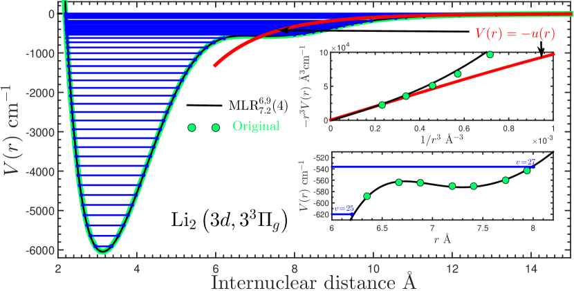
Figure 4: Point-wise original, and analytic MLR potentials for $3d(3^{3}\Pi_{g})$ representing the ab initio calculations of Musial and Kucharski (2014). The top inset shows the long-range behavior in Le Roy space, and the bottom inset shows that the MLR successfully captures the tiny second minimum which has a depth of $\approx 13.5$ cm^-1.

Since the leading term not shown in Eq. 6 is $\frac{u(r)^{2}}{4\mathfrak{D}_{e}}$, the contribution of the $C_{3}$ terms to the long-range form of the potential, will interfere with the desired $C_{6}$ and $C_{8}$ terms, and all $C_{9}$ and $C_{11}$ terms will therefore have spurious contributions from the cross-terms formed by the products of the $C_{3}$ terms with the $C_{6}$ and $C_{8}$ terms respectively. We fix this in the same way as was done for $C_{6}$ and $C_{9}$ in Dattani et al. (2008); Le Roy et al. (2009); Dattani and Le Roy (2011); Semczuk et al. (2013); Gunton et al. (2013); Dattani and LeRoy (2015), by applying a transformation to all $C_{6}$, $C_{9}$, and this time also $C_{11}$ terms:

$$C_{6} \rightarrow C_{6}+\frac{C_{3}^{2}}{4\mathfrak{D}_{e}}$$ (12)

$$C_{9} \rightarrow C_{9}+\frac{C_{3}C_{6}}{2\mathfrak{D}_{e}},$$ (13)

$$C_{11} \rightarrow C_{11}+\frac{C_{3}C_{8}}{2\mathfrak{D}_{e}}.$$ (14)

where the transformation in Eq. 12 has to be made first due to Eq. 13’s dependence on $C_{6}$.

Additionally, the long-range formulas in terms of $C_{m}$ constants in Eqs. 8,10,11 were derived under the assumption that two free atoms are interacting with each other, and there is no overlap of the electrons’ wavefunctions as would be in a bound molecule. To take into account the effect of electron overlap, we use the damping function form from Le Roy et al. (2011):

$$C_{m} \rightarrow C_{m}D_{m}^{(s)}\left(r\right)$$ (15)

$$D_{m}^{(s)}\left(r\right) \equiv \left(1-e^{-\left(\frac{b^{(s)}\rho r}{m}+\frac{c^{(s)}\left(\rho r\right)^{2}}{\sqrt{m}}\right)}\right)^{m+s},$$ (16)

where for interacting atoms A and B, $\rho\equiv\rho_{{\rm AB}}=\frac{2\rho_{{\rm A}}\rho_{{\rm B}}}{\rho_{{\rm A}}\rho_{{\rm B}}},$ in which $\rho_{{\rm X}}\equiv\left(\nicefrac{{I^{{\rm X}}}}{{I^{{\rm H}}}}\right)^{\nicefrac{{2}}{{3}}}$ is defined in terms of the ionization potentials of atom X, denoted $\left(I^{{\rm X}}\right)$, and hydrogen $\left(I^{{\rm H}}\right)$. We use $s=-1$, which as shown in Le Roy et al. (2011), means that the MLR potential has the physically desired behavior $V(r)\simeq\nicefrac{{1}}{{r^{2}}}$ in the limit as $r\rightarrow 0$. For $s=-1$, the system independent parameters take the values $b^{(-1)}=3.30$, and $c^{(-1)}=0.423$ Le Roy et al. (2011).

I.3 Long-range constants

For electronic states of Li₂ approaching the $2S+2P$ asymptote, the $C_{3,6,8}$ constants for all electronic state symmetries have been calculated with finite-mass corrections for ⁶Li and ⁷Li Tang et al. (2009), and even an attempt at relativistic corrections has been made for the $C_{3}$ constants Tang (2015); Tang et al. (2010). Furthermore, for $2S+2P$, third-order perturbation theory has been used to calculate non-relativistic infinite-mass values for $C_{9}$ and $C_{11}$ Tang et al. (2011) , meaning that it was possible to also include the non-relativistic infinite-mass value of $C_{10}$ calculated in Zhang et al. (2007).

The situation is much less convenient for $2S+3P$. No third-order perturbation theory calculation has been done for $C_{9}$ or $C_{11}$, and without $C_{9}$ it does not make sense to include the $C_{10}$ value, which was calculated in the same study as for the $2S+2P$ asymptote Zhang et al. (2007). Also, no finite-mass or relativistic corrections have been calculated for the $C_{3,6,8}$ values associated with $2S+3P$. Nevertheless, we have available the non-relativistic infinite-mass values for $C_{3,6,8}$ that were calculated in Zhang et al. (2007), and these were reported with an order of magnitude higher precision than in the very highly cited 1995 paper of Marinescu and Dalgarno Marinescu and Dalgarno (1995), and only one order of magnitude lower precision than the $2S+2P$ values which are known (see Table 2 in Dattani and LeRoy (2015) for a list of the best known $C_{m}$ constants for each symmetry approaching $2S+2P$). All $C_{m}$ constants that are used in this study for $2S+3P$ are given in Table 2.

Table 2: The best currently available long-range constants for Li₂ electronic states that dissociate to $2S+3P$ (in Hartree atomic units). All values come from Zhang et al. (2007) and were calculated without relativistic corrections, and under the assumption that both Li nuclei have infinite mass.

	${}^{\nicefrac{{1}}{{3}}}\Sigma_{\nicefrac{{u}}{{g}}}$		${}^{\nicefrac{{3}}{{1}}}\Sigma_{\nicefrac{{u}}{{g}}}$		${}^{\nicefrac{{1}}{{3}}}\Pi_{\nicefrac{{u}}{{g}}}$		${}^{\nicefrac{{3}}{{1}}}\Pi_{\nicefrac{{u}}{{g}}}$
$C_{3}$	0.	0033314	$-$0.	0033314	$-$0.	0016657	0.0016657
$C_{6}$	3.	8236$\times 10^{4}$	3.	8236$\times 10^{4}$	2.	0282$\times 10^{4}$	2.0282$\times 10^{4}$
$C_{8}$	2.	4870$\times 10^{7}$	2.	3183$\times 10^{7}$	7.	8976$\times 10^{5}$	3.7222$\times 10^{5}$

 

Table 3: Parameters defining the MLR${}_{p,q}^{r_{{\rm ref}}}(N_{\beta})$ potentials fitted to ab initio points from Musial and Kucharski (2014), and with long-range functions $u(r)$ defined according to the descriptions in section I.3, and with long-range constants presented in Table 2. Numbers in parentheses are 95% confidence limit uncertainties in the last digit(s) shown, calculated from the least-squares fitting procedure.

$3b(3^{3}\Pi_{u})$				$3B(3^{1}\Pi_{u})$		$3C(3^{1}\Pi_{g})$		$3d(3^{3}\Pi_{g})$
MLR${}_{6,7}^{5.9}(17)$				MLR${}_{6,6}^{6.2}(4)$		MLR${}_{6,8}^{7.0}(8)$		MLR${}_{6,9}^{7.2}(4)$
$\mathfrak{D}_{e}$	5765.593  cm-1			$\mathfrak{D}_{e}$	5368.8(38)  cm-1	$\mathfrak{D}_{e}$	$4066.0467$  cm-1	$\mathfrak{D}_{e}$	$6045.135$  cm-1
$r_{e}$	3.984 527(23) Å			$r_{e}$	3.165 8(18) Å	$r_{e}$	3.184 402(23) Å	$r_{e}$	3.	137 142(23) Å
$\beta_{0}$	0.378369938	$\beta_{10}$	-3213.8074	$\beta_{0}$	-0.8509	$\beta_{0}$	0.78516117	$\beta_{0}$	0.	78516117
$\beta_{1}$	0.918196351	$\beta_{11}$	1673.5923	$\beta_{1}$	-0.592	$\beta_{1}$	2.3951022	$\beta_{1}$	2.	39510218
$\beta_{2}$	2.08782371	$\beta_{12}$	6482.429	$\beta_{2}$	-0.038	$\beta_{2}$	6.950787	$\beta_{2}$	6.	9507868
$\beta_{3}$	0.96103485	$\beta_{13}$	-1705.759	$\beta_{3}$	0.74	$\beta_{3}$	-4.68625	$\beta_{3}$	-4.	686246
$\beta_{4}$	-46.0405588	$\beta_{14}$	-7329.75	$\beta_{4}$	0.57	$\beta_{4}$	-5.17796	$\beta_{4}$	-5.	17796
$\beta_{5}$	-117.75187	$\beta_{15}$	822.19			$\beta_{5}$	5.22029
$\beta_{6}$	271.27645	$\beta_{16}$	4297.08			$\beta_{6}$	7.5253
$\beta_{7}$	880.09337	$\beta_{17}$	-122.54			$\beta_{7}$	-2.100

 

II MLR potentials

It has been suggested that fully analytic potentials Huang and Le Roy (2003), and specifically the MLR Pashov (2008) may not have the flexibility required to capture some features such as multiple minima and shelves (see examples of these features appearing in $2S-3P$ potentials of Li₂ in Figs 1-4). While no attempt (as far as I am aware) has thus far been made to use a fully analytic potential to capture such features, an increasing number of applications of the MLR potential after the publications of Huang and Le Roy (2003); Pashov (2008) has made it a strong case for a “universal” potential form. MLR-type potentials have successfully described spectroscopic data for many electronic states of many diatomic molecules Le Roy et al. (2006); Roy and Henderson (2007); Salami et al. (2007); Shayesteh et al. (2007); Le Roy et al. (2009); Coxon and Hajigeorgiou (2010); Stein et al. (2010); Piticco et al. (2010); Le Roy et al. (2011); Ivanova et al. (2011); Dattani and Le Roy (2011); Xie et al. (2011); Yukiya et al. (2013); Knöckel et al. (2013); Semczuk et al. (2013); Wang et al. (2013); Li et al. (2013a); Gunton et al. (2013); Meshkov et al. (2014); Dattani (2014); Coxon and Hajigeorgiou (2015); Walji et al. (2015); Dattani (2015); Dattani and LeRoy (2015); Dattani et al. (2014). It has also become customary to fit ab initio data for diatomic Xiao et al. (2013a, b); Kedziera et al. (2015); Teodoro et al. (2015); You et al. (2015a, b, c) and polyatomic Li and Le Roy (2008); Li et al. (2010); Tritzant-Martinez et al. (2013); Wang et al. (2013); Li et al. (2013b); Ma et al. (2014) systems to MLR models . Therefore, we use the MLR model in this study, and the results here support the idea of the MLR model being a strong candidate for a “universal” model for potential energy curves and surfaces.

All MLR potentials were made by fitting to the ab initio points of Ref. Musial and Kucharski (2014) with the program ${\tt DPotFIT}$ Le Roy et al. (2013). Since this is a non-linear least-squares fitting, ‘starting parameters’ are needed in order to allow ${\tt DPotFit}$ to achieve reasonable fits. Starting parameters were obtained from the program ${\tt BetaFIT}$ Le Roy et al. (2013). When fitting to ab initio points, ${\tt DPotFIT}$ aims to minimize the dimensionless root mean square deviation:

$$dd\equiv\sqrt{\frac{1}{N_{{\rm data}}}\sum_{i=1}^{N_{{\rm data}}}\left(\frac{V_{{\rm MLR}}(i)-V_{{\rm\textit{ab initio}}}(i)}{u_{\textit{ab initio}}(i)}\right)^{2}},$$ (17)

where $V_{{\rm{\rm MLR}}}(i)$ and $V_{{\rm\textit{ab initio}}}(i)$ are the values of the respective potentials at the $i^{{\rm th}}$ internuclear distance value (the order of course does not matter) and $N_{{\rm data}}$ is the total number of ab initio points to which the MLR potential is being fitted. $u_{\textit{ab initio}}(i)$ is the uncertainty in the $i^{{\rm th}}$ ab initio point, so that the MLR potential is likely to lie more closely to ab initio points at distances where the ab initio calculation is expected to be more reliable, and the requirement for the MLR potential to match the ab initio is less harsh in areas where the ab initio calculation is expected to be less accurate.

It is extremely hard to determine accurate estimates on the uncertainties for ab initio points. The ab initio points we are using from Musial and Kucharski (2014) were all calculated with the same basis set (which the authors denoted by ANO-RCC+), therefore there is no indication of the size of the basis set error. Furthermore, all of their calculations were done with the same number of excitations included in their coupled cluster method: FS-CCSD(2,0) only includes 1- and 2-electron excitations, so it would be extremely unlikely to estimate the deviation from the full 6-electron (FCI) limit. Perhaps even more importantly, the calculations of Musial and Kucharski (2014) neglected relativistic, spin-orbit, and non-Born-Oppenheimer effects, so accurately estimating $u_{{\rm\textit{ab initio}}}(i)$ might seem impossible.

However, in my recent benchmark paper Dattani and LeRoy (2015), it was shown that none of the vibrational energies associated with the ab initio potential from Musial and Kucharski (2014) for the $b(1^{3}\Pi_{u})$ state of Li${}_{2},$ deviated from the empirical potential’s vibrational energies by more than 12 cm^-1. Since that ab initio potential used the same basis set and method as their potentials for the electronic states approaching $2S+3P$, I aimed to make $V_{{\rm MLR}}(i)-V_{{\rm\textit{ab initio}}}(i)$ less than 15 cm^-1 for all $i$ except at very small internuclear distances near the $r=0$ singularity where the inner wall of the potential rapidly increases, crosses the dissociation limit, and then attains extremely large energy values. The exact values used for $u_{\textit{ab initio}}(i)$ that were used are presented in Tables 4, 6, 8 and 10. Furthermore, there are places in which it was desirable to make $u_{\textit{ab initio}}(i)$ smaller than 15 cm^-1. This was in places where the potentials from Musial and Kucharski (2014) had features such as tiny second minima, tiny shelves, or any other type of abrupt change. The subsections (below) for each electronic state will describe in detail the nature of these features and how this affected the choice of $u_{\textit{ab initio}}(i)$ (once again the exact values are given in Tables 4, 6, 8 and 10).

The MLR model was fitted to the points from Musial and Kucharski (2014) with various manually adjusted values of the MLR parameters $(N_{{\rm\beta}},p,q,r_{{\rm ref}})$ in search for the lowest $dd$ according to Eq. 17 such that increasing $N_{{\rm\beta}}$ no longer reduced $dd$ significantly further than the best $dd$ obtained with the previous increase in $N_{\beta}$. Details for each electronic state are described in the subsections below which focus on each state.

II.1 The $3b(3^{3}\Pi_{u})$ state

The first $b$ state of Li₂ dissociates to the $2S+2P$ asymptote. A very detailed analysis of theory vs experiment for the first $b$ state of Li₂ was recently reported Dattani and LeRoy (2015), which summarized 14 different experiments providing new information on the $b(1^{3}\Pi_{u})$ state since 1983 Engelke and Hage (1983); Preuss and Baumgartner (1985); Rai et al. (1985); Xie and Field (1985a, b, 1986a); Rice et al. (1986); Rice and Field (1986); Li et al. (1992); Linton et al. (1992); Li et al. (1996c); Weyh et al. (1996); Russier et al. (1997); Lazarov et al. (2001a), and mentioned several other papers that involved this state without providing information on any new levels. Due to the spin-orbit coupling between $b$ states of alkali dimers and their respective $A(^{1}\Sigma_{u}^{+})$ states, recent experimental and theoretical papers have studied the lowest $b$ state of Rb₂, Salami et al. (2007); Drozdova et al. (2013); Tomza et al. (2013), NaCs Zaharova et al. (2009), KCs Kruzins et al. (2010), RbCs Docenko et al. (2010), Cs₂ Bai et al. (2011) and NaK Harker et al. (2015).

It is thus surprising that no experiments have been reported for the second $b$ state of Li₂, which dissociates to the $2P+2P$ asymptote. The present paper is concerned with the third $b$ state, which dissociates to $2S+3P$. The ab initio potential for $3b(3^{3}\Pi_{u})$ from Musial and Kucharski (2014) has a small shelf-like feature before the minimum, and another much longer one closer to dissociation (see Fig. 1). The first shelf is located between $v=0$ and $v=1$, and it lasts from about $3.2-3.6$ Å. The second shelf starts after $v=27$ and lasts from about $6.4-8$ Å. Despite these fairly pronounced shelf features, at the resolution of the ab initio points (which is about $0.1\,\mbox{\AA}$), the $3b$ state only has one minimum!

In Section II it was mentioned that, with the exception of points at very small values of $r$, the goal was to match all ab initio points of Musial and Kucharski (2014) to within $\pm$15 cm^-1 (and points at larger values of $r$ even better), since this was about the level of accuracy found when comparing ab initio points Musial and Kucharski (2014) to an empirical potential for $b(1^{3}\Pi_{u})$ in Dattani and LeRoy (2015). Preliminary fits used such a weighting scheme for the least-squares fitting, except with points comprising the two shelves mentioned in the previous paragraph, weighted with much smaller uncertainties. This was especially important for the second shelf, which only spanned a range of $<100$ cm^-1: Because if the discrepancy between the MLR and ab initio was $-15$ cm^-1 at one point, and $+15$ cm^-1 at another point, the $30$ cm^-1 range of discrepancy would constitute a significant portion of the range of the entire shelf itself. After these preliminary fits, it was found that in order to get the MLR matching the original data with the desired precision, it helped to decrease the uncertainties on the non-shelf ab initio points to slightly below $\pm 15$ cm^-1. The best fits were found with the weights shown in Table 4. Once these final weights were chosen, fits were performed for 252 different combinations of the MLR parameters $(N_{\beta},p,q,r_{{\rm ref}})$, with $4\leq N_{\beta}\leq 17$, $6\leq p\leq 8$, $2\leq q\leq 8$, $(5\leq r_{{\rm ref}}\leq 6.5)$ Å, though not every point in the convex hull formed by these ranges was used. For example, some fits were done with $(p,q)=(6,2)$ and some fits were done with $(p,q)=(8,6)$ but it did not seem necessary to do fits with $(p,q)=(8,2)$. The best fit was found with $(N_{\beta},p,q,r_{{\rm ref}})=(17,6,7,5.9\,$Å), and had $dd=1.548$, while the best fit with $N_{\beta}=16$ was with $(N_{\beta},p,q,r_{{\rm ref}})=(16,6,6,5.3\,\text{\AA})$ and had $dd=2.790$. Apart from in the inner wall of the potential, the worst discrepancy between the MLR and the original points for this $N_{\beta}=16$ case it was $>30$ cm^-1, while for this $N_{\beta}=17$ case was $<11$ cm^-1 so it was quite easy to select the $N_{\beta}=17$ fit. Since this $N_{\beta}=17$ fit satisfied all of our desiderata, $N_{\beta}=18$ fits were not explored.

The final MLR parameters for the chosen case are given in Table 3. The inset of Fig. 1 shows the long-range behavior of the MLR potential and the original ab initio points of Musial and Kucharski (2014) in Le Roy space, and compares them to the theoretical long-range potential based on Eq. 8 and the long-range constants in Table 2. The agreement is surprisingly excellent, however after about 17.7 Å $(1/r^{3}\approx 0.001\,8\,\mbox{\AA}^{-3})$ we see that the original points dip below the theoretical curve, which should not happen because $C_{8}$ is attractive (see Section 4.3 of Roy and Henderson (2007), for example). The fact that the MLR potential matches the theoretical curve in this regard, is yet another advantage of using an MLR to represent the ab initio points. Furthermore, while not shown in Fig. 1, the theoretical long-range curve without damping, matches the damped curve shown in the figure to graphical accuracy at least in the range $14\,\mbox{\AA}\leq r\leq\infty$ $(0\leq 1/r^{3}=0.000\,36\,\mbox{\AA}^{-3})$, so this conclusion about the original points spuriously dipping below the theoretical curve is true whether or not long-range damping is considered.

II.2 The $3B(3^{1}\Pi_{u})$ state

The first $B$ state has a barrier before dissociating to the $2S+2P$ asymptote, and has therefore been the subject of many empirical studies Hessel and Vidal (1979); Russier et al. (1994); Bouloufa et al. (1999); Cacciani and Kokoouline (2000); Bouloufa et al. (2001a, b); Huang and Le Roy (2003). It has also been used to study other states, such as in Bernheim (1982); Barakat et al. (1986); Linton et al. (1990); Kubkowska et al. (2007); Linton et al. (1992). The second $B$ state potential (sometimes called the “$C^{1}\Pi_{u}$ state” rather than the $2B$ state) dissociates to $2P+2P$ and hugs the inside of the first minimum of the $2A(1^{1}\Sigma_{u}^{+})$ potential, and due to the perturbations between these $2B$ and $2A$ states, there have been many empirical studies of the $2B$ state Barrow et al. (1960); Ishikawa et al. (1991); Weyh et al. (1996); Ross et al. (1998); Kasahara et al. (2000); Kubkowska et al. (2007).

The present paper is concerned with third $B$ state. The $3B$ state dissociates to $2S+3P$ and there has only been one experiment which studied the third $B$ state (sometimes called the “$D^{1}\Pi_{u}$ state”) Barrow et al. (1960), which was over 55 years ago! The authors of that work mentioned in their paper that they were not able to confidently assign vibrational quantum numbers to their data, and therefore they were only able to conclude that $T_{e}<34\,140$ cm^-1 and $\omega_{e}\approx 250$ cm^-1. In that study, the anharmonic values $x_{e}\omega_{e}$, equilibrium rotational constants $B_{e}$, and dissociation energies $\mathfrak{D}_{e}$ were determined for the $2B$ state of Li₂ and for the $2B$ and $3B$ states of Na₂, but not for the $3B$ state of Li₂.

It is no surprise that none of the experiments on the $2B$ state showed any indication of a barrier in the potential, because the leading long-range term $(C_{5})$ is attractive Zhang et al. (2007). However, it is perhaps surprising that the ab initio potential of Musial and Kucharski (2014) for the $3B$ state does not have a barrier (at least before the calculations stopped at about 21 Å), because the leading long-range interaction term $(C_{3})$ for this state is repulsive Zhang et al. (2007). There is however a good theoretical explanation for the lack of barrier in the $3B$ state. The long-range potential for $3B$ is not just a simple sum of inverse powers ($-C_{3}/r^{3}-C_{6}/r^{6}\cdots$), but it is the middle eigenvalue of the $3\times 3$ spin-orbit interaction matrix of Eq. 10, which involves the $6a(6^{3}\Sigma_{u})$ and $3b(3^{3}\Pi_{u})$ states. For large internuclear distances, the $6a$ state pushes down on the $3B$ state enough to remove the barrier. Indeed, numerical calculations of the eigenvalues of the $3\times 3$ matrix show that the potential is attractive at all distances (beyond the repulsive inner wall for $r\ll r_{e}$). This $3\times 3$ matrix for $3B$ is the exact same as the one for the first $B$ state, which does have a barrier, but for the $3B$ state the $C_{3}$ is three orders of magnitude smaller than for the first $B$ state, and the $C_{6}$ is one order of magnitude bigger than for the first $B$ state Zhang et al. (2007). This highlights the importance of using the $3\times 3$ coupling matrix because a simple inverse power sum with a negative leading long-range term (such as the negative $C_{3}$ in the present case) is guaranteed to have a barrier, and there was even a barrier when using the middle eigenvalue of the $3\times 3$ coupling matrix for the $2S+2P$ values of $C_{m}$, but the specific values of $C_{m}$ at $2S+3P$ seem to be past a bifurcation point at which the barrier is lost.

Since alkali parent states of $B(^{1}\Pi_{u})$ symmetry only have one spin-orbit daughter state ($\Omega_{u/g}=1_{u})$, we do not need to worry about defining the MLR long-range function $u(r)$ in a piece-wise manner, and it is simply defined as the middle eigenvalue of the $3\times 3$ interaction matrix of Eq. 10. Also, since there are no features such as barriers, multiple minima or shelves, the weighting strategy was straightforward. Preliminary fits were done with all points from Musial and Kucharski (2014) being weighted with uncertainty $\pm 15$ cm^-1 if $V(r)<-100\,$cm^-1, with $\pm 5$ cm^-1 if $V(r)<-20$ cm^-1, with $\pm 1$ cm^-1 if $V(r)<1$ cm^-1 and $\pm 0.5$ cm^-1 for the one point for which $-1$ cm${}^{-1}<V(r)<0$ cm^-1. It was then found that most uncertainties could be even further reduced without making the fitting too difficult, and that for very small values of $r$ it was very difficult to achieve $\pm 15$ cm^-1 agreement in the fit. In the end, the points from Musial and Kucharski (2014) for the smallest values of $r$ (with $V(r)>-4000\,$cm^-1) were weighted with uncertainty $\pm 100$ cm^-1, and all other points were weighted with $\pm 1$ cm^-1, except for the last point which was weighted with $\pm 0.5$ cm^-1 because $V(r)$ itself was only $\approx-0.7$ cm^-1. These final weights are shown in Table 6.

Once these final weights were chosen, fits were performed for 150 different combinations of the MLR parameters $(N_{\beta},p,q,r_{{\rm ref}})$, with $3\leq N_{\beta}\leq 5$, $6\leq p\leq 7$, $2\leq q\leq 7$, $(5\leq r_{{\rm ref}}\leq 10)$ Å, though not every point in the convex hull formed by these ranges was used. The best fit with $N_{\beta}=4$ was with $(p,q,r_{{\rm ref}})=(6,6,6.2\,\text{\AA})$ which had $dd=4.307$ while the best fit found using $N_{\beta}=5$ was only marginally better ($dd=4.128)$ and no fits were found with $N_{\beta}=3$ that had $dd<10$. Therefore, the choice of MLR model for this electronic state was easy to make, and the final parameters are listed in Table 3.

II.3 The $3C(3^{1}\Pi_{g})$ state

The first $C(^{1}\Pi_{g})$ state dissociates to $2S+2P$ and was not studied in detail until 1990 Miller et al. (1990). This was 11 years after the second state of $C(^{1}\Pi_{g})$ symmetry (sometimes called the “$G^{1}\Pi_{g}$ state” since it was given this name in Bernheim (1981)) was studied in detail in 1979 Bernheim et al. (1979). This $2C$ state dissociates to $2P+2P$ and was studied again in a series of follow-up papers by Bernheim et al. Bernheim (1981); Bernheim et al. (1982, 1983). Impressively, empirical spectroscopic constants have also been reported for all Rydberg states in the series $nd\pi^{1}\Pi_{g}$ for $n=3-15$ (!) Bernheim et al. (1982, 1983). In the same paper, it was determined that the $n=3$ state in this series is in fact the $2C$ state.

The third $C$ state is the subject of the present work, since it dissociates to $2S+3P$. It only has one spin-orbit daughter state, which has $1_{g}$ symmetry and couples to the $1_{g}$ daughters of the $3c(3^{3}\Sigma_{g}^{+})$ and $3d(3^{3}\Pi_{g})$ states. The potential energy of the $3C$ state’s $1_{g}$ daughter is given by the middle eigenvalue of the appropriate $3\times 3$ matrix. Preliminary fits were done with the same weighting scheme as for the $3B$ state, except with the points surrounding the second minimum weighted more strongly (with $\pm 0.5$ cm^-1), since the depth of this well is $<10$ cm^-1 and therefore it would not be satisfactory to fit to these points with an agreement of only $\pm 15$ cm^-1! It was then found that many points could be weighted more strongly without making the fitting too difficult. The weights were adjusted to $\pm 10$ cm^-1 for points at the smallest values of $r$ ($V(r)>-3000$ cm^-1), to $\pm 5$ cm^-1 for the rest of the points with $V(r)<-1000$ cm^-1, to $\pm 1$ cm^-1 for points with $V(r)<-1$ cm^-1, except for the points near the second minimum, and the very last point for which $V(r)\approx-0.75$ cm^-1. The final weights are presented in Table 8.

With these final weights, fits were performed for 302 different combinations of the MLR parameters $(N_{\beta},p,q,r_{{\rm ref}})$, with $2\leq N_{\beta}\leq 11$, $6\leq p\leq 11$, $(4\leq r_{{\rm ref}}\leq 12)$ Å, though not every point in the convex hull formed by these ranges was used. The best fit with $N_{\beta}=8$ was with $(p,q,r_{{\rm ref}})=(6,5,7.5\,\text{\AA})$ which had $dd=1.612$, but this potential did not capture the second minimum very well (particularly, it approaches the barrier leading to that minimum with the ab initio point of $V(7.408\,\text{\AA})=-88.76$ cm^-1 being represented with a discrepancy of $>5.5$ cm^-1). The best fit with $N_{\beta}=8$ which captured $V(7.408\,\text{\AA})$ with a discrepancy of $<2$ cm^-1 was with $(p,q,r_{{\rm ref}})=(6,8,7.0\,\text{\AA})$ which had $dd=3.536$. None of the $N_{\beta}=7$ models that reproduced $V(7.408\,\text{\AA})$ with discrepancy $<2$ cm^-1 had an overall $dd<4$, and while $N_{\beta}=9$ fits were found with discrepancies for this point $<2$ cm^-1 and overall $dd$ as low as $2.593$, there were no points beyond $r=2.6$ Å for which the $N_{\beta}=8$ case with $dd=3.536$ misrepresented an original point by $>18$ cm^-1 (the highest discrepancy was $17.37$ cm^-1 at 3.175 Å, and among these $N_{\beta}=9$ cases, the lowest discrepancy for this same point was 12.70 cm^-1). While deciding not to go beyond $N_{\beta}=8$ was not an easy choice, there is not much reason to believe that the calculation in Musial and Kucharski (2014) for $V(3.175\text{}\text{\AA})$ is so precise that representing it more closely by $\approx 5$ cm^-1 is worth adding an extra parameter. Here it is mentioned that while the comparison against the empirical potential in Dattani and LeRoy (2015) for the lowest $b$ state showed no discrepancy of $>12$ cm^-1, that paper also noted the surprisingly small effect of Born-Oppenheimer breakdown in that system, meaning that it is likely that the potentials in Musial and Kucharski (2014) for other electronic states (especially ones approaching $2S-3P$, which seem to interact with each other more than the ones approaching the $2S-2P$ state) will be accurate to slightly less precision than $\pm$12 cm^-1. The final MLR parameters for the chosen model are listed in Table 3.

II.4 The $3d(3^{3}\Pi_{g})$ state

The first $d$ state has a potential energy curve which approaches the $2S+2P$ asymptote, but the ab initio calculations of Musial and Kucharski (2014) indicate that it has no bound states. Therefore, it is no surprise that no bound levels have been found in experiments on this state, though it was indeed involved in some experiments Li et al. (1998); Lazarov et al. (2001b); Dai et al. (2005). While the prediction in Musial and Kucharski (2014) that the first $d$ state has no bound levels is likely to be true, it should be noted that ab initio predictions of this sort are not always reliable. The 1995 ab initio study of Poteau and Spiegelmann (1995) predicted that the $1^{1}\Sigma_{u}^{-}$ state would have no bound levels, but the 2014 calculations of Musial and Kucharski (2014) found there to be a dissociation energy of $\mathfrak{D}_{e}=$14 cm^-1 and an equilibrium harmonic frequency of $\omega_{e}=10$ cm^-1, indicating the existence of at least two bound vibrational levels! Likewise, the 2006 ab initio study of Jasik and Sienkiewicz (2006) found the $1^{3}\Delta_{u}$ state to not have any bound levels, but the earlier 1995 study of Poteau and Spiegelmann (1995) and the 2014 study of Musial and Kucharski (2014) both predicted $\mathfrak{D}_{e}\geq 3430$ cm^-1 and $\omega_{e}\leq 255$ cm^-1.

The second $d$ state has been studied extensively. Spectroscopic measurements for $2d$ were made in Xie and Field (1986a); Yiannopoulou et al. (1995b); Li et al. (1996b, a); Weyh et al. (1996); Russier et al. (1997); Li et al. (2007), and $2d$ was also used in various other experimental studies such as Xie and Field (1985c, 1986b); Rice et al. (1986); Rice and Field (1986); Linton et al. (1992, 1999); Lazarov et al. (2001b); Dai et al. (2005).

The focus of this paper is on the third $d$ state, which is the only $\Lambda=\Pi$ state dissociating to $2S+3P$ for which rovibrationally resolved spectra have been measured, but only 13 lines were observed (with $v=6,7,8,10$) Yiannopoulou et al. (1995b). Hyperfine structure was also studied experimentally for $3d$ in Li et al. (1996b), but it was only for the $N=6,8$ levels of $v=8$, which had already been studied without focus on hyperfine structure in Yiannopoulou et al. (1995b). Finally, the $3d$ state was involved in the experiments of Li et al. (1996a), but the focus of that study was not the $3d$ state.

Since the $3d$ state has four spin-orbit daughter states ($0_{g}^{+},0_{g}^{-},1_{g},2_{g}$, analogous with the $3b$ state), we treat the $2_{g}$ symmetry in this paper, since there is only one state dissociating to $2S+3P$ with $2_{g}$ symmetry and therefore the long-range potential is a simple sum of inverse-power terms rather than a complicated $2\times 2$ or $3\times 3$ interaction matrix. The fitting strategy was very similar to what it was for the $3C$ state, except the $3d$ state seemed to require stronger weighting of the points near the second minimum, and weaker weighting of other points. These final weights are shown in Table 6.

Once these final weights were chosen, fits were performed for 238 different combinations of the MLR parameters $(N_{\beta},p,q,r_{{\rm ref}})$, with $3\leq N_{\beta}\leq 11$, $5\leq p\leq 8$, $2\leq q\leq 10$, $(5\leq r_{{\rm ref}}\leq 7.5)$ Å, though not every point in the convex hull formed by these ranges was used, and it is noted that $p$ must be $\geq 6$ in order to ensure the correct long-range behavior Dattani and Le Roy (2011), but fits with $p=5$ were still instructive to better understand the model dependence for this potential. The best fit with $N_{\beta}=4$ and $p\geq 6$ was with $(p,q,r_{{\rm ref}})=(6,7,7.2\,\text{\AA})$ which had $dd=4.292$, only 0.043 higher than the best fit found with $p=5$. Fits with $N_{\beta}=5$ had $dd$ values as low as $2.972$ but the mentioned $N_{\beta}=4$ case did not misrepresent any of the original points beyond $2.434\,\text{\AA})$ by $>13$ cm^-1, so all desiderata were satisfied without resorting to $N_{\beta}=5$. No $N_{\beta}=3$ cases had $dd<10$, so the choice of MLR model for this electronic state was easy to make, and the final parameters are listed in Table 3.

III Conclusion

Analytic MLR potentials were fitted to the ab initio points from Musial and Kucharski (2014) and with correct long-range behavior incorporated according to effects of spin-orbit coupling described in Eqs. 8, 10, 11 and the long-range constants in Table 2. Despite the potentials from Musial and Kucharski (2014) having unusual features such as multiple minima, barriers, and shelves, which have never been described by an MLR-type model before, all of these features were successfully captured with the MLR model. This answers an age-old question of whether or not fully analytic potentials can have the flexibility needed in order to capture such features. Pashov’s 2008 paper “Pointwise and analytic potentials for diatomic molecules. An attempt for critical comparison” Pashov (2008) described lack of flexibility as one of the three drawbacks of analytic potentials, and suggested that the MLR model may not be able to capture double minima or shelf-like features. Five years earlier in 2003, Huang and Le Roy suggested in Huang and Le Roy (2003) that Pashov’s pointwise approach would be the method of choice for potentials such as those described in this paper:

“A particular strength of [Pashov’s pointwise] model is the fact that it has more local flexibility than do fully analytical potential function forms, in that a shift of one potential point has only a modest effect on the function outside its immediate neighborhood. This would tend to make [Pashov’s pointwise] model the method of choice for cases where the potential has substantial local structure or undergoes an abrupt change of character on a small fraction of the overall interval, such as occurs near an avoided curve crossing. In contrast, a change in one of the parameters defining a [fully analytic] such as our DELR function will in general affect the potential across the whole domain. This makes the parameters defining [fully analytic] potentials very highly correlated and can give rise to difficulty in achieving full unique convergence in a fit.”

At the time when this quote was written, the MLR model did not exist yet, and at the time of Pashov’s paper Pashov (2008), only a primitive (less flexible) form of the MLR existed, which was used in just four simple cases of ground electronic states Le Roy et al. (2006); Roy and Henderson (2007); Salami et al. (2007); Shayesteh et al. (2007). It is possible that the notion that analytic potentials cannot capture such special features may be attributed to the lack of diversity in attempted applications at that early stage in time, and the lack of some of the newer MLR features which were introduced in Le Roy et al. (2009) and Le Roy et al. (2011) for increasing flexibility, and in Dattani et al. (2008) for correcting the long-range behavior.

This paper also represents, to the best of my knowledge, the most detailed study of analytic potentials for excited electronic molecular states.

References

- (1)
- (2)
- Xie and Field (1986a) X. Xie and R. Field, Journal of Molecular Spectroscopy 117, 228 (1986a).
- Yiannopoulou et al. (1995a) A. Yiannopoulou, K. Urbanski, A. M. Lyyra, L. Li, B. Ji, J. T. Bahns, and W. C. Stwalley, The Journal of Chemical Physics 102, 3024 (1995a).
- Li et al. (2007) D. Li, F. Xie, L. Li, A. Lazoudis, and A. M. Lyyra, Journal of Molecular Spectroscopy 246, 180 (2007).
- Bernheim et al. (1983) R. A. Bernheim, L. P. Gold, and T. Tipton, The Journal of Chemical Physics 78, 3635 (1983).
- Song et al. (2002) M. Song, P. Yi, X. Dai, Y. Liu, L. Li, and G.-H. Jeung, Journal of Molecular Spectroscopy 215, 251 (2002).
- Yiannopoulou et al. (1995b) A. Yiannopoulou, K. Urbanski, S. Antonova, A. M. Lyyra, L. Li, T. An, T. J. Whang, B. Ji, X. T. Wang, W. C. Stwalley, T. Leininger, and G.-H. Jeung, The Journal of Chemical Physics 103, 5898 (1995b).
- Li et al. (1996a) L. Li, S. Antonova, A. Yiannopoulou, K. Urbanski, and A. M. Lyyra, The Journal of Chemical Physics 105, 9859 (1996a).
- Li et al. (1996b) L. Li, A. Yiannopoulou, K. Urbanski, A. M. Lyyra, B. Ji, W. C. Stwalley, and T. An, The Journal of Chemical Physics 105, 6192 (1996b).
- Ivanov et al. (1999) V. Ivanov, V. Sovkov, L. Li, A. Lyyra, G. Lazarov, and J. Huennekens, Journal of molecular spectroscopy 194, 147 (1999).
- Sebastian et al. (2014) J. Sebastian, C. Gross, K. Li, H. C. J. Gan, W. Li, and K. Dieckmann, Physical Review A 90, 033417 (2014).
- Semczuk et al. (2013) M. Semczuk, X. Li, W. Gunton, M. Haw, N. S. Dattani, J. Witz, A. K. Mills, D. J. Jones, and K. W. Madison, Physical Review A 87, 052505 (2013).
- Gunton et al. (2013) W. Gunton, M. Semczuk, N. Dattani, and K. Madison, Physical Review A 88, 062510 (2013).
- Tang et al. (2011) L.-Y. Tang, Z.-C. Yan, T.-Y. Shi, and J. Mitroy, Physical Review A 84 (2011), 10.1103/PhysRevA.84.052502.
- Mitroy et al. (2010) J. Mitroy, M. S. Safronova, and C. W. Clark, Journal of Physics B: Atomic, Molecular and Optical Physics 43, 202001 (2010).
- Cronin et al. (2009) A. D. Cronin, J. Schmiedmayer, and D. E. Pritchard, Reviews of Modern Physics 81, 1051 (2009).
- Dattani and LeRoy (2015) N. S. Dattani and R. J. LeRoy, Journal of Chemical Physics (2015).
- Dattani and Le Roy (2011) N. S. Dattani and R. J. Le Roy, Journal of Molecular Spectroscopy 268, 199 (2011).
- Le Roy et al. (2009) R. J. Le Roy, N. S. Dattani, J. A. Coxon, A. J. Ross, P. Crozet, and C. Linton, The Journal of Chemical Physics 131, 204309 (2009).
- Aubert-Frécon et al. (1998) M. Aubert-Frécon, G. Hadinger, S. Magnier, and S. Rousseau, Journal of Molecular Spectroscopy 188, 182 (1998).
- Bussery and Aubert-Frecon (1985) B. Bussery and M. Aubert-Frecon, The Journal of Chemical Physics 82, 3224 (1985).
- Aubert-Frécon (2015) M. Aubert-Frécon, Private Communication (2015).
- Brown et al. (2013) R. C. Brown, S. Wu, J. V. Porto, C. J. Sansonetti, C. E. Simien, S. M. Brewer, J. N. Tan, and J. D. Gillaspy, Physical Review A 87, 032504 (2013).
- Sansonetti et al. (2011) C. J. Sansonetti, C. E. Simien, J. D. Gillaspy, J. N. Tan, S. M. Brewer, R. C. Brown, S. Wu, and J. V. Porto, Physical Review Letters 107, 023001 (2011).
- Sansonetti et al. (1995) C. Sansonetti, B. Richou, R. Engleman, and L. Radziemski, Physical Review A 52, 2682 (1995).
- Schmidt-Mink et al. (1985) I. Schmidt-Mink, W. Müller, and W. Meyer, Chemical Physics 92, 263 (1985).
- Poteau and Spiegelmann (1995) R. Poteau and F. Spiegelmann, Journal of Molecular Spectroscopy 171, 299 (1995).
- Jasik and Sienkiewicz (2006) P. Jasik and J. Sienkiewicz, Chemical Physics 323, 563 (2006).
- Musial and Kucharski (2014) M. Musial and S. A. Kucharski, Journal of Chemical Theory and Computation 10, 1200 (2014).
- Lee (2014) C.-W. Lee, Bulletin of the Korean Chemical Society 35, 1422 (2014).
- Bubin et al. (2009) S. Bubin, M. Stanke, and L. Adamowicz, The Journal of chemical physics 131, 044128 (2009).
- Dattani (2015) N. S. Dattani, Journal of Molecular Spectroscopy 311, 76 (2015).
- Bubin and Adamowicz (2007) S. Bubin and L. Adamowicz, The Journal of Chemical Physics 126, 214305 (2007).
- Koput (2011) J. Koput, The Journal of chemical physics 135, 244308 (2011).
- Komasa et al. (2011) J. Komasa, K. Piszczatowski, G. Lach, M. Przybytek, B. Jeziorski, and K. Pachucki, Journal of Chemical Theory and Computation 7, 3105 (2011).
- Pachucki and Komasa (2012) K. Pachucki and J. Komasa, The Journal of chemical physics 137, 204314 (2012).
- Noga and Bartlett (1987) J. Noga and R. J. Bartlett, The Journal of Chemical Physics 86, 7041 (1987).
- Hirata and Bartlett (2000) S. Hirata and R. J. Bartlett, Chemical Physics Letters 321, 216 (2000).
- Kallay and Surjan (2001) M. Kallay and P. R. Surjan, The Journal of Chemical Physics 115, 2945 (2001).
- Kallay and Gauss (2004) M. Kallay and J. Gauss, The Journal of chemical physics 120, 6841 (2004).
- Evangelista et al. (2006) F. A. Evangelista, W. D. Allen, and H. F. Schaefer, The Journal of chemical physics 125, 154113 (2006).
- DeYonker and Allen (2012) N. J. DeYonker and W. D. Allen, The Journal of chemical physics 137, 234303 (2012).
- DeYonker and Shah (2014) N. J. DeYonker and S. A. Shah, Theoretical Chemistry Accounts 133, 1518 (2014).
- LeRoy (1973) R. J. LeRoy, Molecular Spectroscopy Molecular Spectroscopy, 1, 113 (1973).
- LeRoy (1974) R. J. LeRoy, Canadian Journal of Physics 52, 246 (1974).
- Ji et al. (1995) B. Ji, C.-C. Tsai, and W. C. Stwalley, Chemical Physics Letters 236, 242 (1995).
- Zhang et al. (2007) J.-Y. Zhang, J. Mitroy, and M. Bromley, Physical Review A 75 (2007), 10.1103/PhysRevA.75.042509.
- Dattani et al. (2008) N. S. Dattani, R. J. LeRoy, A. J. Ross, and C. Linton, in Proceedings of the International Symposium on Molecular Spectroscopy (2008) p. RC11.
- Le Roy et al. (2011) R. J. Le Roy, C. C. Haugen, J. Tao, and H. Li, Molecular Physics 109, 435 (2011).
- Tang et al. (2009) L.-Y. Tang, Z.-C. Yan, T.-Y. Shi, and J. Babb, Physical Review A 79 (2009), 10.1103/PhysRevA.79.062712.
- Tang (2015) L.-Y. Tang, Private Communication (2015).
- Tang et al. (2010) L.-Y. Tang, Z.-C. Yan, T.-Y. Shi, and J. Mitroy, Physical Review A 81 (2010), 10.1103/PhysRevA.81.042521.
- Marinescu and Dalgarno (1995) M. Marinescu and A. Dalgarno, Physical Review A 52, 311 (1995).
- Huang and Le Roy (2003) Y. Huang and R. J. Le Roy, The Journal of Chemical Physics 119, 7398 (2003).
- Pashov (2008) A. Pashov, Proceedings of the International Symposium on Molecular Spectroscopy (2008).
- Le Roy et al. (2006) R. J. Le Roy, Y. Huang, and C. Jary, The Journal of Chemical Physics 125, 164310 (2006).
- Roy and Henderson (2007) R. J. L. Roy and R. D. E. Henderson, Molecular Physics 105, 663 (2007).
- Salami et al. (2007) H. Salami, A. J. Ross, P. Crozet, W. Jastrzebski, P. Kowalczyk, and R. J. Le Roy, The Journal of Chemical Physics 126, 194313 (2007).
- Shayesteh et al. (2007) A. Shayesteh, R. D. E. Henderson, R. J. Le Roy, and P. F. Bernath, The Journal of Physical Chemistry. A 111, 12495 (2007).
- Coxon and Hajigeorgiou (2010) J. A. Coxon and P. G. Hajigeorgiou, The Journal of Chemical Physics 132, 094105 (2010).
- Stein et al. (2010) A. Stein, H. Knöckel, and E. Tiemann, The European Physical Journal D 57, 171 (2010).
- Piticco et al. (2010) L. Piticco, F. Merkt, A. A. Cholewinski, F. R. McCourt, and R. J. Le Roy, Journal of Molecular Spectroscopy 264, 83 (2010).
- Ivanova et al. (2011) M. Ivanova, A. Stein, A. Pashov, A. V. Stolyarov, H. Knöckel, and E. Tiemann, The Journal of Chemical Physics 135, 174303 (2011).
- Xie et al. (2011) F. Xie, L. Li, D. Li, V. B. Sovkov, K. V. Minaev, V. S. Ivanov, A. M. Lyyra, and S. Magnier, The Journal of Chemical Physics 135, 024303 (2011).
- Yukiya et al. (2013) T. Yukiya, N. Nishimiya, Y. Samejima, K. Yamaguchi, M. Suzuki, C. D. Boone, I. Ozier, and R. J. Le Roy, Journal of Molecular Spectroscopy 283, 32 (2013).
- Knöckel et al. (2013) H. Knöckel, S. Rühmann, and E. Tiemann, The Journal of Chemical Physics 138, 094303 (2013).
- Wang et al. (2013) L. Wang, D. Xie, R. J. Le Roy, and P.-N. Roy, The Journal of Chemical Physics 139, 034312 (2013).
- Li et al. (2013a) G. Li, I. E. Gordon, P. G. Hajigeorgiou, J. A. Coxon, and L. S. Rothman, Journal of Quantitative Spectroscopy and Radiative Transfer 130, 284 (2013a).
- Meshkov et al. (2014) V. V. Meshkov, A. V. Stolyarov, M. C. Heaven, C. Haugen, and R. J. LeRoy, The Journal of Chemical Physics 140, 064315 (2014).
- Dattani (2014) N. S. Dattani, physics.chem-ph , arXiv:1408.3301 (2014).
- Coxon and Hajigeorgiou (2015) J. A. Coxon and P. G. Hajigeorgiou, Journal of Quantitative Spectroscopy and Radiative Transfer 151, 133 (2015).
- Walji et al. (2015) S.-D. Walji, K. M. Sentjens, and R. J. Le Roy, The Journal of chemical physics 142, 044305 (2015).
- Dattani et al. (2014) N. S. Dattani, L. N. Zack, M. Sun, E. R. Johnson, R. J. Le Roy, and L. M. Ziurys, physics.chem-ph , arXiv:1408.2276 (2014).
- Xiao et al. (2013a) K.-L. Xiao, C.-L. Yang, M.-S. Wang, X.-G. Ma, and W.-W. Liu, Journal of Quantitative Spectroscopy and Radiative Transfer 129, 8 (2013a).
- Xiao et al. (2013b) K.-L. Xiao, C.-L. Yang, M.-S. Wang, X.-G. Ma, and W.-W. Liu, The Journal of chemical physics 139, 074305 (2013b).
- Kedziera et al. (2015) D. Kedziera, L. Mentel, P. S. Zuchowski, and S. Knoop, Physical Review A 91, 062711 (2015).
- Teodoro et al. (2015) T. Q. Teodoro, R. L. A. Haiduke, U. Dammalapati, S. Knoop, and L. Visscher, The Journal of Chemical Physics 143, 084307 (2015).
- You et al. (2015a) Y. You, C.-L. Yang, M.-S. Wang, X.-G. Ma, W.-W. Liu, and L.-Z. Wang, Journal of Quantitative Spectroscopy and Radiative Transfer 165, 56 (2015a).
- You et al. (2015b) Y. You, C.-L. Yang, M.-S. Wang, X.-G. Ma, W.-W. Liu, and L.-Z. Wang, Spectrochimica Acta Part A: Molecular and Biomolecular Spectroscopy (2015b), 10.1016/j.saa.2015.09.004.
- You et al. (2015c) Y. You, C.-L. Yang, M.-S. Wang, X.-G. Ma, and W.-W. Liu, Physical Review A 92, 032502 (2015c).
- Li and Le Roy (2008) H. Li and R. J. Le Roy, Physical Chemistry Chemical Physics : PCCP 10, 4128 (2008).
- Li et al. (2010) H. Li, P.-N. Roy, and R. J. Le Roy, The Journal of Chemical Physics 133, 104305 (2010).
- Tritzant-Martinez et al. (2013) Y. Tritzant-Martinez, T. Zeng, A. Broom, E. Meiering, R. J. Le Roy, and P.-N. Roy, The Journal of Chemical Physics 138, 234103 (2013).
- Li et al. (2013b) H. Li, X.-L. Zhang, R. J. Le Roy, and P.-N. Roy, The Journal of Chemical Physics 139, 164315 (2013b).
- Ma et al. (2014) Y.-T. Ma, T. Zeng, and H. Li, The Journal of chemical physics 140, 214309 (2014).
- Le Roy et al. (2013) R. J. Le Roy, J. Y. Seto, and Y. Huang, “DPotFit 2.0: A Computer Program for Fitting Diatomic Molecule Spectra to Potential Energy Functions (University of Waterloo Chemical Physics Research Report CP-667),” (2013).
- Engelke and Hage (1983) F. Engelke and H. Hage, Chemical Physics Letters 103, 98 (1983).
- Preuss and Baumgartner (1985) W. Preuss and G. Baumgartner, Zeitschrift fur Physik A Atoms and Nuclei 320, 125 (1985).
- Rai et al. (1985) S. Rai, B. Hemmerling, and W. Demtröder, Chemical Physics 97, 127 (1985).
- Xie and Field (1985a) X. Xie and R. W. Field, The Journal of Chemical Physics 83, 6193 (1985a).
- Xie and Field (1985b) X. Xie and R. W. Field, Chemical Physics 99, 337 (1985b).
- Rice et al. (1986) S. F. Rice, X. Xie, and R. W. Field, Chemical Physics 104, 161 (1986).
- Rice and Field (1986) S. F. Rice and R. W. Field, in Methods of Laser Spectroscopy, edited by Y. Prior, A. Ben-Reuven, and M. Rosenbluh (1986) pp. 389–398.
- Li et al. (1992) L. Li, T. An, T.-J. Whang, A. M. Lyyra, W. C. Stwalley, R. W. Field, and R. A. Bernheim, The Journal of Chemical Physics 96, 3342 (1992).
- Linton et al. (1992) C. Linton, R. Bacis, P. Crozet, F. Martin, A. Ross, and J. Verges, Journal of Molecular Spectroscopy 151, 159 (1992).
- Li et al. (1996c) L. Li, S. Antonova, A. Yiannopoulou, K. Urbanski, and A. M. Lyyra, The Journal of Chemical Physics 105, 9859 (1996c).
- Weyh et al. (1996) T. Weyh, K. Ahmed, and W. Demtröder, Chemical Physics Letters 248, 442 (1996).
- Russier et al. (1997) I. Russier, A. Yiannopoulou, P. Crozet, A. Ross, F. Martin, and C. Linton, Journal of Molecular Spectroscopy 184, 129 (1997).
- Lazarov et al. (2001a) G. Lazarov, A. Lyyra, and L. Li, Journal of molecular spectroscopy 205, 73 (2001a).
- Drozdova et al. (2013) A. N. Drozdova, A. V. Stolyarov, M. Tamanis, R. Ferber, P. Crozet, and A. J. Ross, Physical Review A 88, 022504 (2013).
- Tomza et al. (2013) M. Tomza, W. Skomorowski, M. Musial, R. Gonzalez-Ferez, C. P. Koch, and R. Moszynski, Molecular Physics (2013).
- Zaharova et al. (2009) J. Zaharova, M. Tamanis, R. Ferber, A. N. Drozdova, E. A. Pazyuk, and A. V. Stolyarov, Physical Review A 79, 012508 (2009).
- Kruzins et al. (2010) A. Kruzins, I. Klincare, O. Nikolayeva, M. Tamanis, R. Ferber, E. A. Pazyuk, and A. V. Stolyarov, Physical Review A 81, 042509 (2010).
- Docenko et al. (2010) O. Docenko, M. Tamanis, R. Ferber, T. Bergeman, S. Kotochigova, A. V. Stolyarov, A. de Faria Nogueira, and C. E. Fellows, Physical Review A 81, 042511 (2010).
- Bai et al. (2011) J. Bai, E. H. Ahmed, B. Beser, Y. Guan, S. Kotochigova, A. M. Lyyra, S. Ashman, C. M. Wolfe, J. Huennekens, F. Xie, D. Li, L. Li, M. Tamanis, R. Ferber, A. Drozdova, E. Pazyuk, A. V. Stolyarov, J. G. Danzl, H.-C. Nägerl, N. Bouloufa, O. Dulieu, C. Amiot, H. Salami, and T. Bergeman, Physical Review A 83, 032514 (2011).
- Harker et al. (2015) H. Harker, P. Crozet, A. J. Ross, K. Richter, J. Jones, C. Faust, J. Huennekens, A. V. Stolyarov, H. Salami, and T. Bergeman, Physical Review A 92, 012506 (2015).
- Hessel and Vidal (1979) M. M. Hessel and C. R. Vidal, The Journal of Chemical Physics 70, 4439 (1979).
- Russier et al. (1994) I. Russier, F. Martin, C. Linton, P. Crozet, A. Ross, R. Bacis, and S. Churassy, Journal of Molecular Spectroscopy 168, 39 (1994).
- Bouloufa et al. (1999) N. Bouloufa, P. Cacciani, R. Vetter, and A. Yiannopoulou, The Journal of Chemical Physics 111, 1926 (1999).
- Cacciani and Kokoouline (2000) P. Cacciani and V. Kokoouline, Physical Review Letters 84, 5296 (2000).
- Bouloufa et al. (2001a) N. Bouloufa, P. Cacciani, V. Kokoouline, F. Masnou-Seeuws, R. Vetter, and L. Li, Physical Review A 63, 042507 (2001a).
- Bouloufa et al. (2001b) N. Bouloufa, P. Cacciani, R. Vetter, A. Yiannopoulou, F. Martin, and A. J. Ross, The Journal of Chemical Physics 114, 8445 (2001b).
- Bernheim (1982) R. A. Bernheim, The Journal of Chemical Physics 76, 57 (1982).
- Barakat et al. (1986) B. Barakat, R. Bacis, S. Churassy, R. Field, J. Ho, C. Linton, S. Mc Donald, F. Martin, and J. Vergès, Journal of Molecular Spectroscopy 116, 271 (1986).
- Linton et al. (1990) C. Linton, F. Martin, R. Bacis, and J. Vergès, Journal of Molecular Spectroscopy 142, 340 (1990).
- Kubkowska et al. (2007) M. Kubkowska, A. Grochola, W. Jastrzebski, and P. Kowalczyk, Chemical Physics 333, 214 (2007).
- Barrow et al. (1960) R. F. Barrow, N. Travis, and C. V. Wright, Nature 187, 141 (1960).
- Ishikawa et al. (1991) K. Ishikawa, S. Kubo, and H. Kato, The Journal of Chemical Physics 95, 8803 (1991).
- Ross et al. (1998) A. Ross, P. Crozet, C. Linton, F. Martin, I. Russier, and A. Yiannopoulou, Journal of Molecular Spectroscopy 191, 28 (1998).
- Kasahara et al. (2000) S. Kasahara, P. Kowalczyk, M. H. Kabir, M. Baba, and H. Kato, The Journal of Chemical Physics 113, 6227 (2000).
- Miller et al. (1990) D. A. Miller, L. P. Gold, P. D. Tripodi, and R. A. Bernheim, The Journal of Chemical Physics 92, 5822 (1990).
- Bernheim (1981) R. A. Bernheim, The Journal of Chemical Physics 74, 2749 (1981).
- Bernheim et al. (1979) R. A. Bernheim, L. P. Gold, P. B. Kelly, C. Kittrell, and D. K. Veirs, Physical Review Letters 43, 123 (1979).
- Bernheim et al. (1982) R. Bernheim, L. Gold, and T. Tipton, Chemical Physics Letters 92, 13 (1982).
- Li et al. (1998) L. Li, G. Lazarov, and A. Lyyra, Journal of Molecular Spectroscopy 191, 387 (1998).
- Lazarov et al. (2001b) G. Lazarov, A. Lyyra, and L. Li, Journal of molecular spectroscopy 205, 73 (2001b).
- Dai et al. (2005) X. Dai, E. A. Torres, E.-B. W. Lerch, D. J. Wilson, and S. R. Leone, Chemical Physics Letters 402, 126 (2005).
- Xie and Field (1985c) X. Xie and R. W. Field, The Journal of Chemical Physics 83, 6193 (1985c).
- Xie and Field (1986b) X. Xie and R. Field, Journal of Molecular Spectroscopy 117, 228 (1986b).
- Linton et al. (1999) C. Linton, F. Martin, A. Ross, I. Russier, P. Crozet, A. Yiannopoulou, L. Li, and A. Lyyra, Journal of molecular spectroscopy 196, 20 (1999).
- (132)