Cosmological reconstruction and Om diagnostic analysis of Einstein-Aether Theory

Abstract

In this paper, we will analyse the cosmological models in Einstein-aether gravity, which is a modified theory of gravity in which a time-like vector field breaks the Lorentz symmetry. We will use this formalism to analyse different cosmological models with different behavior of the scale factor. In this analysis, we will use a certain functional dependence of the dark energy on the Hubble parameter. It will be demonstrated that the aether vector field has a non-trivial effect on these cosmological models. We will also perform the Om diagnostic in Einstein-aether gravity. Thus, we will fit parameters of the cosmological models using recent observational data.

1 Introduction

The Lorentz symmetry is one of the most important symmetries in nature, and all particle physics experiments have demonstrated that this symmetry is not broken at the scale at which such experiments are performed. However, it is predicted from quantum gravity that the Lorentz symmetry should break down at Planck scale, where even the manifold structure of spacetime breaks down due to quantum fluctuations. In fact, almost all approaches to quantum gravity predict that the local Lorentz symmetry of spacetime only exists in some IR limit of the theory. So, the Lorentz symmetry is expected to break in the UV limit. It may be noted that it has been explicitly demonstrated that such a breaking of Lorentz symmetry in the UV limit occur in the discrete spacetime [1], models based on string field theory [2], spacetime foam [3], spin-network in loop quantum gravity (LQG) [4], non-commutative geometry [6, 5], and ghost condensation in perturbative quantum gravity [7]. As the Lorentz symmetry fixes the form of the energy-momentum dispersion relation, the breaking of Lorentz symmetry in the UV limit, will also lead to a modification of the energy-momentum dispersion relation in the UV limit. In fact, there are indications from the Greisen-Zatsepin-Kuzmin limit (GZK limit) t the usual energy-momentum relation will get modified in the UV limit [8, 9]. The Pierre Auger Collaboration and the High Resolution Fly’s Eye (HiRes) experiment have confirmed earlier results of the GZK cutoff [10]. So, it is possible that the Lorentz symmetry will break in the UV limit, and only occur as an effective symmetry in the IR limit. Thus, it is important to construct a theory, such that it will reproduce the general relativity in the IR limit, and break the local Lorentz symmetry in the UV limit. Such a theory has been constructed by using different Lifshitz scaling for space and time, and this theory is called the Horava-Lifshitz gravity [11, 12]. This original proposal for the Horava-Lifshitz gravity improves the renormalization of gravity, as it differs from general relativity in the UV limit. However, there are several problems associated with this proposal, and these include the problems associated with instabilities, overconstrained evolution, and strong coupling at low energies [13]-[18]. These problems occur due to a badly behaved scalar mode of gravity, which is produced by the presence of a nondynamical spatial foliation in the action. To resolve this problem, an extension of Horava-Lifshitz gravity called the BPSH theory has been proposed [19]. It has been demonstrated that the BPSH theory is equivalent to general relativity coupled to a dynamical unit timelike vector field [20]. Here the vector is restricted in the action to be hypersurface orthogonal.

The phenomenology and observational constraints on the coupling parameters of Einstein-aether gravity have been studied [21]. It may also be noted that constraints on Einstein-aether gravity from binary pulsars have also been discussed [22]. In this work, the consequences of Lorentz symmetry, which occur in Einstein-aether gravity, on the orbital evolution of binary pulsars. In the focus of this study was on the dissipative effects in such a process. It was observed that the breaking of the Lorentz symmetry modified such effects. Thus, the orbital dynamics of binary pulsars was also modified in Einstein-aether gravity. Such a modification causes the emission of dipolar radiation, and this made the orbital separation decrease faster than in general relativity. The quadruple component of the emission was also modified. The orbital evolution depends critically on the sensitivities of the stars, as this measure how their binding energies depend on the motion relative to the preferred frame. In this study such sensitivities have also been numerically calculated in Einstein-aether gravity. These predictions have been compared with observations, and this has been used to set constraints on Einstein-aether gravity.

It has been demonstrated that the Einstein-aether theory can be analysed in the framework of the metric-affine gravity [23]. Such a formalism resembles the gauge theory of theory. In this formalism, the aether vector field is related to certain post-Riemannian nonmetricity pieces contained in an independent linear connection of spacetime. Black hole solution have also been studied in the Einstein-aether gravity. It has been demonstrated that the deviations from the Schwarzschild metric are typically only a few percent for most of the explored parameter regions, and this makes it difficult to observe with electromagnetic probes, but they can be detected using gravitational wave detectors [24]. As gravitational wave detectors are going to be used extensively in future astronomy, it is interesting to study the implications of Einstein-aether gravity.

As the Einstein-aether gravity, introduce a time like vector field, they are expected to modify the cosmological evolution of the universe. In fact, various different solution for the accelerating universe in the Einstein-aether gravity have been studied [25]. These solutions have been used to analyse the inflationary behaviour of the early universe and late-time cosmological acceleration. It has been demonstrated that the aether field produces accelerated expansion in situations where inflation would not occur in general relativity. Hence, the aether field can effect the inflation in a very non-trivial way. The cosmological evolution of cosmological models based on Einstein-aether gravity with power-law potential have also been studied [26]. The cosmological models have also been studied in the Einstein-aether gravity coupled to a Galileon type scalar field [27]. It was observed that in such models, the universe experiences a late time acceleration, for pressure-less baryonic matter. It may be noted that gravitational wave can be used to analyse the cosmological aspects of Einstein-aether gravity. This is because it has been demonstrated that for cosmological models based Einstein-aether gravity, a direct correspondence exists between perfect fluids carrying anisotropic stress and a modification in the propagation of gravitational waves [28]. As the anisotropic stress can be measured in a model-independent manner, the gravitational waves can be used to obtain constraints on the cosmological models in the Einstein-aether gravity. Even though several studies have been done on the Einstein-aether gravity, it is important to perform an extensive study of how this modification of general relativity can change cosmological models, and how it fits with the current data. This is important as many aspects of Einstein-aether gravity can be detected using gravitational waves, and in near future, it is expected that the gravitational wave will be used to study many of these interesting phenomena. So, in this paper, we perform a detail study on the modification of different cosmological models from Einstein-aether gravity. These models have been studied in general relativity, and we will, and we will analyse them in the Einstein-aether gravity. So, in this paper, we will first use the reconstruction technique to find some viable forms for Einstein-aether gravity. We obtain the expressions of the modified Friedmann equations and from these equations, we can find the effective density and the effective pressure for the Einstein-aether gravity. We will also fit the model with observational data. This will be done by using the cosmographic analysis involving the Om parametrization. We will also use the SnIa, BAO and Hubble data to find the $1\sigma$ and $2\sigma$ contours for density parameter $\Omega_{m}$ arising from the Sne Ia + BAO.

2 Einstein-aether Gravity

In this section, we will review the main features of the Einstein-aether gravity. It may be noted that Einstein-aether gravity is equivalent to the BPSH generalization to the Horava-Lifshitz gravity [20], and so it breaks the Lorentz symmetry. However, the cosmology described by this theory would still be described by the standard Friedmann equations with an additional matter contribution [25]. This is because the breaking of Lorentz symmetry occurs due to a time-like vector field in the Einstein-aether theory, and so the cosmological effects can be obtained by analysing the correction to the standard Friedmann equations from this additional time-like vector field. The action $S$ of the Einstein-aether gravity is given by [29, 30],

$$S=\int d^{4}x\sqrt{-g}\left[\frac{R}{4\pi G}+L_{EA}+L_{m}\right],$$ (2.1)

where $L_{EA}$ indicates the Lagrangian density of the aether vector field, while $L_{m}$ indicates the Lagrangian density of the usual matter fields. The Lagrangian density of the aether vector field $L_{EA}$ can be expressed as

$$L_{EA} = \frac{M^{2}}{16\pi G}F\left(K\right)+\frac{1}{16\pi G}\lambda\left(A^{a}A_{a}+1\right),$$ (2.2)

$$K = M^{-2}K^{ab}_{cd}\nabla_{a}A^{c}\nabla_{b}A^{d},$$ (2.3)

$$K^{ab}_{cd} = c_{1}g^{ab}g_{cd}+c_{2}\delta_{c}^{a}\delta_{d}^{b}+c_{3}\delta_{d}^{a}\delta_{c}^{b},\ \ a,b=0,1,2,3$$ (2.4)

where $c_{1}$, $c_{2}$ and $c_{3}$ are three dimensionless constant parameters, $M$ is a coupling constant parameter, $\lambda$ is a Lagrangian multiplier, and $A^{a}$ is a contravariant vector. Here $F\left(K\right)$ is an arbitrary function of the parameter $K$, and a function of the Hubble parameter $H$.
Now using Eq. (2.1), the field equations, for this theory, can be written as [29, 30]

$$G_{ab} = T_{ab}^{Einstein-aether}+8\pi GT_{ab}^{m},$$ (2.5)

$$\nabla_{a}\left(F^{\prime}J^{a}_{\,b}\right) = 2\lambda A_{b},$$ (2.6)

where

$$F^{\prime} = \frac{dF}{dK},$$ (2.7)

$$J^{a}_{\,b}= - 2K^{ad}_{\,\,bc}\nabla_{d}A^{c}.$$ (2.8)

Here $T_{ab}^{m}$ is the energy-momentum tensors for the matter field, and $T_{ab}^{Einstein-aether}$ is the energy-momentum tensor for the aether vector field,

$$T_{ab}^{m} = \left(p+\rho\right)u_{a}u_{b}+pg_{ab},$$ (2.9)

$$T_{ab}^{Einstein-aether} = \frac{1}{2}\nabla_{d}\left[\left(J_{a}^{\,d}A_{b}-J^{d}_{\,a}A_{b}-J_{\left(ab\right)}A^{d}\right)F^{\prime}\right]$$ (2.10)

$$-Y_{\left(ab\right)}F^{\prime}+\frac{1}{2}g_{ab}M^{2}F+\lambda A_{a}A_{b}.$$

Here $\rho$ is the energy density and $p$ is the pressure of the matter. Also $u_{a}$ is defined as $u_{a}=\left(1,0,0,0\right)$, and so it represents the four-velocity vector of the fluid, $A^{a}=\left(1,0,0,0\right)$. It may be noted that it is represented by a time-like unitary vector. Now we define $Y_{ab}$ as

$$Y_{ab}=-c_{1}\left[\left(\nabla_{d}A_{a}\right)\left(\nabla^{d}A_{b}\right)-\left(\nabla_{a}A_{d}\right)\left(\nabla_{a}A^{d}\right)\right].$$ (2.11)

The subscript $\left(ab\right)$ indicates a symmetry with respect to the two indices.

We consider a Friedmann-Robertson-Walker (FRW) metric, which is given by

$$ds^{2}=-dt^{2}+a^{2}\left(t\right)\left[\frac{dr^{2}}{1-kr^{2}}+r^{2}\left(d\theta^{2}+\sin^{2}\theta d\phi^{2}\right)\right],$$ (2.12)

where $a\left(t\right)$ represents the scale factor (which gives useful information about the expansion rate of the universe), $t$ is the cosmic time, and $k$ is the curvature parameter. Here its value can be $-1$, $0$ or $+1$ corresponding to an open, a flat, or a closed Universe. The range of $\theta$ and $\phi$ are $0\leq\theta\leq\pi$ and $0\leq\phi\leq 2\pi$. The four coordinates $\left(r,t,\theta,\phi\right)$ are also known as co-moving coordinates.

Using Eqs. (2.3) and (2.4), we can easily obtain the following general expression for the parameter $K$ [29, 30],

$$K=\frac{3\varepsilon H^{2}}{M^{2}},$$ (2.13)

where $\varepsilon$ is a constant parameter while $H=\dot{a}/a$ is the Hubble parameter. So, using Eq. (2.5), we obtain the Friedmann equations modified by the Einstein-aether gravity,

$$\varepsilon\left(-F^{\prime}+\frac{F}{2K}\right)H^{2}+\left(H^{2}+\frac{k}{a^{2}}\right) = \frac{8\pi G}{3}\rho,$$ (2.14)

$$\varepsilon\frac{d}{dt}\left(HF^{\prime}\right)+\left(-2\dot{H}+\frac{2k}{a^{2}}\right) = 8\pi G\left(p+\rho\right).$$ (2.15)

The conservation equation can now be written as

$$\dot{\rho}+3H\left(p+\rho\right)=0,$$ (2.16)

where the $\dot{\rho}$ indicates a temporal derivative of $\rho$.

We denote the effective energy density in Einstein-aether gravity by $\rho_{EA}$, and the effective pressure in Einstein-aether gravity by $p_{EA}$. So, we can rewrite Eqs. (2.14) and (2.15) as

$$\left(H^{2}+\frac{k}{a^{2}}\right) = \frac{8\pi G}{3}\rho+\frac{1}{3}\rho_{EA},$$ (2.17)

$$\left(-2\dot{H}+\frac{2k}{a^{2}}\right) = 8\pi G\left(p+\rho\right)+\left(\rho_{EA}+p_{EA}\right).$$ (2.18)

Therefore, comparing Eqs. (2.14) and (2.15) with Eqs. (2.17) and (2.18), we can write

$$\rho_{EA} = 3\varepsilon H^{2}\left(F^{\prime}-\frac{F}{2K}\right),$$ (2.19)

$$p_{EA} = -3\varepsilon H^{2}\left(F^{\prime}-\frac{F}{2K}\right)-\varepsilon\left(\dot{H}F^{\prime}+H\dot{F}^{\prime}\right)$$ (2.20)

$$= -\rho_{EA}-\frac{\dot{\rho}_{EA}}{3H}.$$

Using Eq. (2.19), we obtain

$$F^{\prime}-\frac{F}{2K}=\frac{\rho_{EA}}{3\varepsilon H^{2}}.$$ (2.21)

This is equivalent to the following master equation (using the expression of $3\varepsilon H^{2}$ derived from Eq. (2.13)),

$$F^{\prime}-\frac{F}{2K}=\frac{\rho_{EA}}{KM^{2}}.$$ (2.22)

Here that a prime ^′ indicates a derivative with respect to $K$, and so we have $F^{\prime}=\frac{dF}{dK}$.
Using the expressions for $\rho_{EA}$ and $p_{EA}$ given by Eqs. (2.19) and (2.20), we obtain that the EoS parameter $\omega_{EA}$ for the Einstein-aether gravity,

$$\omega_{EA}=\frac{p_{EA}}{\rho_{EA}}=-1-\frac{\left(\dot{H}F^{\prime}+H\dot{F}^{\prime}\right)}{3H^{2}\left(F^{\prime}-\frac{F}{2K}\right)}.$$ (2.23)

3 Models for Dark Energy

The astrophysical data obtained from distant Ia supernovae, large scale structure, baryon acoustic oscillations, weak lensing and cosmic microwave background indicate the existence of dark energy [31, 32, 33, 34, 35, 36, 37, 38, 39, 40]. In this paper, we will analyse the dark energy models using Einstein-aether gravity. The effective density and the effective pressure produced by Einstein-aether gravity can be used to generate dark energy, if the condition $\rho_{EA}+3p_{EA}<0$ is satisfied (i.e., if the strong energy condition is violated). Thus, we obtain

$$2H^{2}\left(F^{\prime}-\frac{F}{2K}\right)>-\left(\dot{H}F^{\prime}+H\dot{F}^{\prime}\right).$$ (3.1)

This is the equation can be used to analyse dark energy in Einstein-aether gravity. So, to analyse the effect of dark energy on cosmological models in the Einstein-aether gravity, we can use $F\left(K\right)$ and $\omega_{Einstein-aether}$. It may be noted that the modified effective Friedmann equation can be written as

$$8\pi G\rho_{darkenergy}=\Sigma_{\Sigma n_{i}=n}A(X,Y,...)\frac{\partial^{n}f(X,Y,...)}{\partial X^{n_{1}}\partial Y^{n_{2}}...}.$$ (3.2)

where $f(X,Y,...)$ is the matter part $K$ action. For a model of dark energy , for example, the holographic dark energy, we have $\rho_{darkenergy}=\rho_{darkenergy}(H,\dot{H},..)$. We can also write it as $\rho_{darkenergy}=\rho_{darkenergy}(X,Y,...)$. So, if we can solve the partial differential equations for $f(X,Y,...)$, we can obtain the effect of dark energy on such cosmological models.

The generalized Nojiri-Odintsov Holographic dark energy models can be used to analyse the dependence of the dark energy on the Hubble parameter [59]. In fact, using the Granda-Oliveros model [41], which is a specific kind of Nojiri-Odintsov Holographic dark energy model, we can write,

$$L_{GO}=\left(\alpha H^{2}+\beta\dot{H}\right)^{-\frac{1}{2}},$$ (3.3)

where $H={\dot{a}}/{a}$ is the Hubble parameter, and $\dot{H}$ is the temporal derivative of $H$. This model is characterized by two constant parameters $\alpha$ and $\beta$. As the dark energy dominates the present cosmological epoch, and its contribution to cosmological epoch near the Big Bang was negligible (i.e. the amount of dark energy increased with the expansion of the universe), the energy density can be assumed to be a function of the Hubble parameter $H$ and its temporal derivative. Such a dependence is characterized by these two parameters. There are other physical reasons which motivate the Granda-Oliveros model. This is because if the IR cut-off chosen is given by the particle horizon, the Holographic dark energy models are not able to produce an accelerated expansion for the present cosmological epoch. However, if the future event horizon is used an the IR cut-off, then the Holographic dark energy models have a problem with causality. It is possible to resolve both these problems by using Granda-Oliveros model [41]. It may be noted that in the limiting case $\left\{\alpha,\beta\right\}=\left\{2,1\right\}$, $L_{GO}$ becomes proportional to the Ricci scalar curvature $L_{GO}\propto R$. However, based on the observational data, such a choice is not physical. This is because the values for these parameters which best fit the observational data have been obtained [42]. These value for a non-flat universe are given by [42],

$$\alpha=0.8824^{+0.2180}_{-0.1163}(1\sigma)\,^{+0.2213}_{-0.1378}(2\sigma), \beta=0.5016^{+0.0973}_{-0.0871}(1\sigma)\,^{+0.1247}_{-0.1102}(2\sigma).$$ (3.4)

These value for a flat universe are given by [42],

$$\alpha=0.8502^{+0.0984}_{-0.0875}(1\sigma)\,^{+0.1299}_{-0.1064}(2\sigma), \beta=0.4817^{+0.0842}_{-0.0773}(1\sigma)\,^{+0.1176}_{-0.0955}(2\sigma).$$ (3.5)

It may be noted that for Granda-Oliveros model, energy density $\rho_{D}$ can be written as

$$\rho_{D} = 3c^{2}\left(\alpha H^{2}+\beta\dot{H}\right).$$ (3.6)

In this paper, we will analyse the effect of Einstein-aether gravity on the cosmological evolution using the Granda-Oliveros model. We will analyse this for different models for the evolution of the scale factor of the universe, and analyse such a model for the observationally motivated values of $\alpha$ and $\beta$.

It may be noted the Granda-Oliveros model has been generalized to a Chen-Jing model [43]. In this cosmological model, the dark energy is a function of the Hubble parameter squared (i.e. $H^{2}$) and its first and second temporal derivatives of the Hubble parameter $\dot{H}$ and $\ddot{H}$,

$$\rho_{D}=3c^{2}\left[\alpha\left(\frac{\ddot{H}}{H}\right)+\beta\dot{H}+\gamma H^{2}\right],$$ (3.7)

where $\alpha$, $\beta$ and $\gamma$ represent three arbitrary dimensionless parameters. The inverse of the Hubble parameter, i.e. $H^{-1}$, is introduced in the first of the three terms of Eq. (3.7), so that each of these three terms have the dimensions.
It may be noted that in the limiting case corresponding to $\alpha=0$, we recover the energy density of dark energy given by the Granda-Oliveros model [44],[45]. Furthermore, in the limiting case, $\alpha=0$, $\beta=1$ and $\gamma=2$, we obtain the expression of the energy density of dark energy with the IR cut-off proportional to the average radius of the Ricci scalar curvature, $L\propto R^{-1/2}$ (when $k=0$). In this paper we will analyse this model for various cosmological model, with different evolution of the scale factor. We will obtain general expression for various parameters for this dark energy model, and they can be compared to various observational data.

4 Cosmological Models

In this section, we will analyse the behavior of various cosmological models in Einstein-aether gravity. These will correspond to different evolution of the scale factor. We will analyse them for the Granda-Oliveros model, using the values obtained from observation. We will also analyse them for the Chen-Jing model.

Now we start by considering the the power-law cosmology. This cosmological model is interesting proposal for the evolution of the scalar factor, and it has been motivate by the existence of the flatness and horizon problems in the standard cosmology [46]. In this cosmological model, it is possible to assume the following form for the evolution of the scale factor,

$$a\left(t\right)=a_{0}t^{m}.$$ (4.1)

where $a_{0}$ is the present day value of $a\left(t\right)$. It is also important to only consider $m>0$, and this will produce an accelerating universe [46]. It may be noted that for $m>1$, the power-law cosmology can solve the horizon problem, the flatness problem, and the problem associated with age of the early universe [47, 48]. The power-law cosmology has been used for analysing the cosmological behavior in modified theories of gravity [49, 50]. Now for Einstein-aether gravity, it is possible to analyse the Granda-Oliveros cut-off for power-law cosmological model. Thus, for a non-flat universe, we obtain,

$$F\left(K\right) = \frac{2c^{2}K(0.8824m-0.5016)}{\varepsilon m}+C_{1}\sqrt{K}.$$ (4.2)

For a flat universe, we obtain,

$$F\left(K\right) = \frac{2c^{2}K(0.8502m-0.4817)}{\varepsilon m}+C_{1}\sqrt{K}.$$ (4.3)

It is also possible to analyse the power-law cosmology using the Chen-Jing model, we have

$$F\left(K\right) = \frac{2c^{2}K\left[2\alpha+n(n\beta+\gamma)\right]}{\varepsilon n^{2}}+C_{4}\sqrt{K}.$$ (4.4)

In this section, $C_{i}$ will denote integration constants, for example, here $C_{1},C_{4}$ denotes the integration constants.

It is also possible to consider a different kind of power law [51, 52],

$$a\left(t\right)=a_{0}(t_{s}-t)^{-n},$$ (4.5)

where $n>0$ and $t<t_{s}$. Such models have a future singularity at finite time, and this is denoted by $t_{s}$. The Granda-Oliveros cut-off for such model can be analysed for both a flat universe and a non-flat universe. For a non-flat universe, we obtain

$$F\left(K\right) = \frac{2c^{2}K(0.8824n+0.5016)}{\varepsilon n}+C_{3}\sqrt{K}.$$ (4.6)

For a flat universe, we obtain

$$F\left(K\right) = \frac{2c^{2}K(0.8502n+0.4817)}{\varepsilon n}+C_{3}\sqrt{K}.$$ (4.7)

Now using Chen-Jing model, we obtain

$$F\left(K\right)=\frac{2c^{2}K\left[2\alpha+n(n\beta+\gamma)\right]}{\varepsilon n^{2}}+C_{4}\sqrt{K},$$ (4.8)

It is also possible to analyse intermediate inflation in Einstein-aether gravity. The intermediate inflation has been used to obtain exact analytic solutions for a given class of potentials for the inflation. The scale factor for intermediate inflation can be expressed as [53, 54],

$$a\left(t\right)=e^{Bt^{\theta}},$$ (4.9)

where $B>0$ and $0<\theta<1$. For a non-flat universe, we have

$$F\left(K\right) = 2(B\varepsilon\theta)^{-1}c^{2}K\left(\frac{KM^{2}}{3B^{2}\varepsilon\theta^{2}}\right)^{\frac{-\theta}{2(-1+\theta)}}$$ (4.10)

$$\times\left[-0.5016(-1+\theta)^{2}+0.8824B\theta\left(\frac{KM^{2}}{3B^{2}\varepsilon\theta^{2}}\right)^{\frac{\theta}{2(-1+\theta)}}\right]$$

$$+\sqrt{K}C_{7}.$$

For a flat universe, we have

$$F\left(K\right) = 2(B\varepsilon\theta)^{-1}c^{2}K\left(\frac{KM^{2}}{3B^{2}\varepsilon\theta^{2}}\right)^{\frac{-\theta}{2(-1+\theta)}}$$ (4.11)

$$\times\left[-0.4817(-1+\theta)^{2}+0.8502\theta\left(\frac{KM^{2}}{3B^{2}\varepsilon\theta^{2}}\right)^{\frac{\theta}{2(-1+\theta)}}\right]$$

$$+\sqrt{K}C_{7}.$$

Now for Chen-Jing model, we obtain

$$F\left(K\right) = \varepsilon^{-1}2\ 3^{-4^{\theta}\left(\frac{1}{-1+\theta}\right)^{-2\theta}-2^{1-\theta}\left(\frac{1}{-1+\theta}\right)^{\theta}}c^{2}K\left(\frac{KM^{2}}{B^{2}\varepsilon\theta^{2}}\right)^{4^{\theta}\left(\frac{1}{-1+\theta}\right)^{-2\theta}}$$ (4.13)

$$\times\left\{\frac{2^{\theta}\beta\left(\frac{1}{-1+\theta}\right)^{2\theta}\left(\frac{KM^{2}}{B^{2}\varepsilon\theta^{2}}\right)^{2^{1-\theta}\left(\frac{1}{-1+\theta}\right)^{\theta}}}{2^{1+3\theta}+2^{\theta}\left(\frac{1}{-1+\theta}\right)^{2\theta}+4\left(\frac{1}{-1+\theta}\right)^{3\theta}}\right.$$

$$\left.+\frac{2^{\theta}3^{2^{-\theta}\left(\frac{1}{-1+\theta}\right)^{\theta}}\gamma\left(\frac{1}{-1+\theta}\right)^{-1+2\theta}\left(\frac{KM^{2}}{B^{2}\varepsilon\theta^{2}}\right)^{2^{-\theta}\left(\frac{1}{-1+\theta}\right)^{\theta}}}{2^{1+3\theta}B\theta+2^{\theta}B\left(\frac{1}{-1+\theta}\right)^{2\theta}\theta+2B\left(\frac{1}{-1+\theta}\right)^{3\theta}\theta}\right.$$

$$\left.+\frac{3^{2^{1-\theta}\left(\frac{1}{-1+\theta}\right)^{\theta}}\alpha\left(2-3\theta+\theta^{2}\right)}{B^{2}\left[1+2^{1+2\theta}\left(\frac{1}{-1+\theta}\right)^{-2\theta}\right]\theta^{2}}\right\},$$

$$+C_{8}\sqrt{K}.$$

It is possible to analyse universes with no past time-like singularity. In such cosmological models, the universe in the infinite past there exists a static state of cosmology, and this state evolves into an inflationary stage. The scale factor for such cosmological models can be expressed as [55, 56],

$$a\left(t\right)=A\left(B+e^{nt}\right)^{\lambda}$$ (4.14)

where $A$, $B$, $n$ and $\lambda$ are four positive constant parameters. In order to avoid singularities, we have to use $B>0$. Furthermore, for for the positivity of scale factor, we have to use $A>0$. It may be noted that in this model, for $a<0$ or $\lambda<0$, a singularity exists. So, for the expanding model, we have to only consider $a>0$ and $\lambda>0$. Using the Granda-Oliveros cut-off for this model, we can analyse a flat universe and a non-flat universe. So, for a non-flat universe, we have

$$F\left(K\right) = \frac{c^{2}K\left(1.7648\lambda-1.0032+0.5016\sqrt{\frac{3\varepsilon n^{2}\lambda^{2}}{KM^{2}}}\log K\right)}{\varepsilon\lambda}$$ (4.15)

$$+\sqrt{K}C_{5}.$$

For a flat universe, we have

$$F\left(K\right) = \frac{c^{2}K\left(1.7004\lambda-0.9634+0.4817\sqrt{\frac{3\varepsilon n^{2}\lambda^{2}}{KM^{2}}}\log K\right)}{\varepsilon\lambda}$$ (4.16)

$$+\sqrt{K}C_{5}.$$

We can also use the Chen-Jing model, and obtain

$$F\left(K\right) = c^{2}(\varepsilon M^{2}\lambda^{2})^{-1}\left[-6\varepsilon n^{2}\alpha\lambda^{2}+2KM^{2}\left(2\alpha-\gamma\lambda+\beta\lambda^{2}\right)\right.$$ (4.17)

$$\left.+\sqrt{3}KM^{2}\sqrt{\frac{\varepsilon n^{2}\lambda^{2}}{KM^{2}}}\left(-3\alpha+\gamma\lambda\right)\log K\right],$$

$$+C_{6}\sqrt{K}.$$

It is possible to analyse matter dominated universe and the accelerated phase of the universe using a single formalism [57, 58]. In such cosmological models, the Hubble constant is given by [59, 60]

$$H(t)=H_{0}+\frac{H_{1}}{t},$$ (4.18)

where $H_{0}$ and $H_{1}$ are two constant parameters. In this case, for the non-flat universe, we obtain

$$F\left(K\right) = -2c^{2}(9\varepsilon M^{2}H_{1})^{-1}[-9.0288\varepsilon^{2}KM^{2}H_{0}-13.5431\varepsilon H_{0}^{2}$$ (4.19)

$$+KM^{2}(0.5016\varepsilon^{3}KM^{2}-7.9416H_{1})$$

$$+\sqrt{K}C_{10}.$$

Furthermore, for the flat universe, we obtain

$$F\left(K\right) = -2c^{2}(9\varepsilon M^{2}H_{1})^{-1}[-8.6706\varepsilon^{2}KM^{2}H_{0}-13.0059\varepsilon H_{0}^{2}$$ (4.20)

$$+KM^{2}(0.4817\varepsilon^{3}KM^{2}-7.5618H_{1})]$$

$$+\sqrt{K}C_{10}.$$

Now using the Chen-Jing model, we obtain

$$F(K) = \sqrt{K}\left[C_{11}+\,{\frac{2{c}^{2}{M}^{2}\alpha\,{K}^{3/2}}{\epsilon\,{H_{{1}}}^{2}}}-{\frac{{c}^{2}{M}^{2}\beta\,{K}^{3/2}}{\epsilon\,H_{{1}}}}\right.$$

$$\left.+{\frac{{c}^{2}{M}^{2}\gamma\,{K}^{3/2}}{\epsilon}}-\,{\frac{9{c}^{2}\sqrt{2}MH_{{0}}\alpha\,K}{\sqrt{\epsilon}{H_{{1}}}^{2}}}+\,{\frac{3{c}^{2}\sqrt{2}MH_{{0}}\beta\,K}{\sqrt{\epsilon}H_{{1}}}}\right.$$

$$\left.+\,{\frac{18\sqrt{2\epsilon}{c}^{2}{H_{{0}}}^{2}H\alpha\,\ln\left(K\right)}{{H_{{1}}}^{2}M}}-\,{\frac{3\sqrt{2\epsilon}{c}^{2}{H_{{0}}}^{2}H\beta\,\ln\left(K\right)}{H_{{1}}M}}\right.$$

$$\left.-\,{\frac{6\sqrt{2\epsilon}{c}^{2}\alpha\,{H_{{0}}}^{3}\ln\left(K\right)}{{H_{{1}}}^{2}M}}\right].$$

The quantum deformed de Sitter ($q$-de Sitter) solution has been obtained by a quantum deformation of the quantum deformation of the conformal group [61]. In fact, the $q$-deformed de Sitter solution has also been used in the analyzing of dS/CFT correspondence and the entanglement entropy for such a solution has also been obtained [61]. The $q$-de Sitter has also been used for analyzing cosmology [62]. Now we will analyse this model for the $q$-de Sitter scale factor [62],

$$a(t)=e_{q}(H_{0}t)=\Big{[}1+(q-1)H_{0}t\Big{]}^{\frac{1}{q-1}}.$$ (4.22)

In this model it is possible to interpolate between the cosmological model based on a power-law and the cosmological model involving de Sitter spacetime. In fact, for early times, $H_{0}t\gg 1$, we obtain

$$a_{early}(t)\sim\Big{[}H_{0}t\Big{]}^{\frac{1}{q-1}}=t^{p}.$$ (4.23)

It is possible to have an acceleration expansion, when $p>1$, and $q<2$. So, we can write

$$a_{early}(t)\preceq e_{q}(H_{0}t)\preceq a_{dS}(t).$$ (4.24)

This inequality, given in Eq. (4.24), produces interesting cosmological evolution in $q$-de Sitter. The $q$-de Sitter can be used to smoothly connect the early cosmological epoch to late time evolution universe. Now we can analyse such a model for a non-flat universe as

$$F(K) = 6c^{2}H_{0}^{2}\left(\frac{K}{\varepsilon H_{0}^{2}}\right)^{1+\frac{1}{-2+q}}\left[\left(\frac{K}{\varepsilon H_{0}^{2}}\right)^{\frac{1}{-2+\frac{2}{-1+q}}}\right]^{\frac{1}{-1+q}}$$ (4.25)

$$\times\left[e^{\frac{q\left((-2+q)\log[K]+\log\left[\frac{K}{\varepsilon H_{0}^{2}}\right]+2(-2+q)\log\left[\left(\frac{K}{\varepsilon H_{0}^{2}}\right)^{-\frac{-1+q}{2(-2+q)}}\right]\right)}{2(-2+q)^{2}(-1+q)}}\right.$$

$$\left.\times K^{-\frac{q}{4-6q+2q^{2}}}\left(\frac{K}{\varepsilon H_{0}^{2}}\right)^{-\frac{-1+2q}{2(-2+q)^{2}(-1+q)}}0.8824\right.$$

$$\left.\times-\frac{(-2+q)^{2}\cdot 0.5016}{-1+q}\right]M^{-2}+\sqrt{K}C_{11}.$$

We can also analyse such a model for the flat universe as

$$F(K) = 6c^{2}H_{0}^{2}\left(\frac{K}{\varepsilon H_{0}^{2}}\right)^{1+\frac{1}{-2+q}}\left[\left(\frac{K}{\varepsilon H_{0}^{2}}\right)^{\frac{1}{-2+\frac{2}{-1+q}}}\right]^{\frac{1}{-1+q}}$$ (4.26)

$$\times\left[e^{\frac{q\left((-2+q)\log[K]+\log\left[\frac{K}{\varepsilon H_{0}^{2}}\right]+2(-2+q)\log\left[\left(\frac{K}{\varepsilon H_{0}^{2}}\right)^{-\frac{-1+q}{2(-2+q)}}\right]\right)}{2(-2+q)^{2}(-1+q)}}\right.$$

$$\left.\times K^{-\frac{q}{4-6q+2q^{2}}}\left(\frac{K}{\varepsilon H_{0}^{2}}\right)^{-\frac{-1+2q}{2(-2+q)^{2}(-1+q)}}0.8502\right.$$

$$\left.\times-\frac{(-2+q)^{2}\cdot 0.4817}{-1+q}\right]M^{-2}+\sqrt{K}C_{11}.$$

We can use the Chen-Jing model, and obtain

$$F(K) = \sqrt{K}C_{13}+\,{\frac{3{c}^{2}\left(2\,\alpha\,{q}^{2}-4\,\alpha\,q+2\,\alpha-\beta\,q+\beta+\gamma\right)}{\epsilon}}K.$$

Thus, we can see the Einstein-aether gravity modifies the cosmological evolution in various different model, with different evolution of scale factor. Hence, this deformation is almost a universal feature of Einstein-aether gravity. We have calculated $F(K)$ for these different cosmological models. Thus, these cosmological model directly depend on the aether vector field. It is also possible to calculate $L_{GO}$, $\omega_{EA}$, $\rho_{EA}$ and $p_{EA}$ for these various different cosmological models. It can be argued that these quantities will also depend on the aether field (see Appendix). Hence, the breaking of Lorentz symmetry by the introduction of a time-like aether vector field can modify the cosmological dynamics in a non-trivial way. Here we explicitly calculated such a modification for a large number of cosmological models.

5 Om Diagnostic Analysis

In this section, we will perform the Om diagnostic analysis of various different cosmological models. The cosmological parameters like the Hubble parameter $H$, deceleration parameter $q$, and the Equation of State (EoS) parameter $\omega$ are important to understand the behavior of cosmological models. It is theoretically and observationally known that different dark energy models produce a positive Hubble parameter and a negative deceleration parameter (i.e. $H>0$ and $q<0$, for the present cosmological epoch. So, $H$ and $q$ can not be used to effectively differentiate between the different dark energy models. Therefore, a higher order of time derivatives of $a(t)$ is required to analyse the dark energy models [66, 65]. So, third order temporal derivative of $a(t)$ can be used to resolve the problem that most dark energy models produce $H>0$ and $q<0$ for the present cosmological epoch. So, now the statefinder parameters $\left\{r,s\right\}$, can be expressed as

$$r = \frac{\dddot{a}}{aH^{3}},$$ (5.1)

$$s = \frac{r-1}{3\left(q-1/2\right)},$$ (5.2)

where $q$ represents the deceleration parameter, which is given by

$$q=-\frac{1}{H^{2}}\frac{\ddot{a}}{a}.$$ (5.3)

An alternative way to write $r$ and $s$ is as

$$r = 1+3\frac{\dot{H}}{H^{2}}+\frac{\ddot{H}}{H^{3}},$$ (5.4)

$$s = -\frac{3H\dot{H}+\ddot{H}}{3H\left(2\dot{H}+3H^{2}\right)}$$ (5.5)

$$= -\frac{3\dot{H}+\ddot{H}/H}{3\left(2\dot{H}+3H^{2}\right)}.$$

It may be noted that statefinder parameters $\left\{r,s\right\}=\left\{1,0\right\}$ represents the point where the flat $\Lambda$CDM model exists in the $r-s$ plane [67]. So, the departure of dark energy models from this fixed point can be used to obtain the distance of these models from the flat $\Lambda$CDM model, taken as reference model.
We also note that in the $\left\{r,s\right\}$ plane, a positive value of the parameter $s$ (i.e. $s>0$) indicates a quintessence-like model of dark energy, and a negative value of the parameter $s$ (i.e. $s<0$) indicates a phantom-like model of dark energy . Furthermore, the evolution from phantom to quintessence is obtained by crossing of the point $\left\{r,s\right\}=\left\{1,0\right\}$ in the $\left\{r,s\right\}$ plane [68].
So, different cosmological models, like the models with a cosmological constant $\Lambda$, braneworld models , chaplygin gas and quintessence models, have been studied using such an analysis [66]. In this study, it was argued that $\left\{r,s\right\}$ can be used to differentiate between different models. An analysis based on $\left\{r,s\right\}$ has also been used to differentiate between dark energy and modified gravity [69, 68].
An important geometrical diagnostic which can be used to for such analysis is called the Om diagnostic analysis [70]. Usually in the study of the statefinder parameters $r$ and $s$, higher order temporal derivatives of $a(t)$ are used. However, in the Om diagnostic analysis only first order temporal derivative are used. This is because it only involves the Hubble parameter, and the Hubble parameter depends on a single time derivative of $a(t)$. So, the Om diagnosis can be considered as a simpler diagnostic than the statefinder diagnosis [71]. It may be noted that the Om diagnosis has also been applied to Galileons models [72, 73]. This set of parameters can now be represented as

$$Om(z)=\frac{\left[\frac{H(z)}{H_{0}}\right]^{2}-1}{(1+z)^{3}-1}.$$ (5.6)

For a constant EoS parameter $\omega$, the expression for $Om(z)$ is given by

$$Om(z)=\Omega_{m0}+(1-\Omega_{m0})\frac{(1+z)^{3(1+\omega)}-1}{(1+z)^{3}-1},$$ (5.7)

Thus, we observe that we have different values of $Om(z)=\Omega_{m0}$ for the $\Lambda$CDM model, quintessence, and phantom cosmological models. In Figure 1, we plot the first cosmological parameters $r-s$, $r-q$, $m-\omega_{Einstein-aether}$ for power-law in the redshift $t=(1+z)^{-1/m}$ range $0.07\leq z\leq 2.3$. A continuous behavior is observed. For $r-s$, we observe that when $r$ is increasing, $s$ is starting to decreasing monotonically, never vanishes. A similar pattern is repeating but in the negative range for $q$. As we observe, the observational value for $q\approx-0.67$ exists in this model. In Figure 2, we plot $Om(z)$ for power-law in the redshift $t=(1+z)^{-1/m}$ range $0.07\leq z\leq 2.3$. We observe that when the redshift $z$ is increasing within the interval $0.07\leq z\leq 2.3$, the $Om(z)$ is decreasing monotonically. For all power exponents $m\neq 2$, always $Om(z)>\Omega_{m0}$, so the model mimics a quintessence with effective EoS $w>-1$.

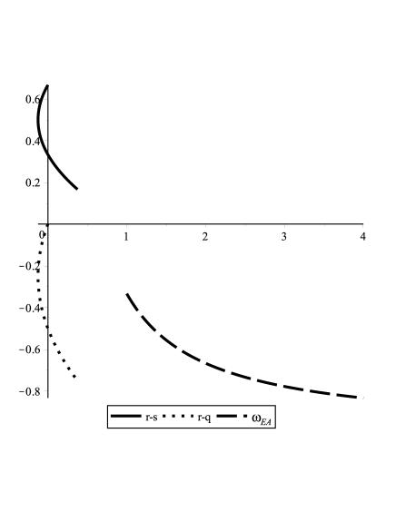
Figure 1: $r-s$, $r-q$, $m-\omega_{Einstein-aether}$ for power-law in the redshift $t=(1+z)^{-1/m}$ range $0.07\leq z\leq 2.3$.

Figure 2: $Om(z)$ for power-law in the redshift $t=(1+z)^{-1/m}$ range $0.07\leq z\leq 2.3$.

In Figure 3, we plot the first cosmological parameters $r-s$, $r-q$, $\omega_{Einstein-aether}$ for a cosmological model with a future singularity. In the redshift $t=t_{s}-(1+z)^{1/n}$ range $0.07\leq z\leq 2.3$, a continuous behavior is observed. For $r-s$, we observe that when $r$ is increasing, $s$ is starting to decreasing monotonically, always remains negative. A similar pattern is repeating but in the negative ranges for $r,q$. As we see, the observational value for $q\approx-0.67$ do not exist in this model. In Figure 4, we plot $Om(z)$ for future singularities model in the redshift $t=t_{s}-(1+z)^{1/n}$ range $0.07\leq z\leq 2.3$. We observe that when the redshift $z$ is increasing within the interval $0.07\leq z\leq 2.3$, the $Om(z)$ is decreasing monotonically, always $Om(z)>\Omega_{m0}$. So, the model with future singularity mimics a quintessence with effective EoS $w>-1$.

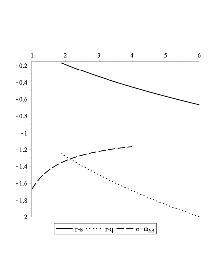
Figure 3: r-s, r-q, $\omega_{Einstein-aether}$ for model with future singularity in the redshift $t=t_{s}-(1+z)^{1/n}$ range $0.07\leq z\leq 2.3$.

Figure 4: $Om(z)$ for model with future singularity in the redshift $t=t_{s}-(1+z)^{1/n}$ range $0.07\leq z\leq 2.3$.

In Figure 5, we plot the first cosmological parameters $r-s$, $r-q$, $\omega_{Einstein-aether}$ for models of emergent universe, in the redshift $t=\ln\left({{\rm e}^{-{\frac{\ln\left(A+zA\right)}{\lambda}}}}-B\right){n}^{-1}$ range $0.07\leq z\leq 2.3$. A continuous behavior is observed. For $r-s$, we observe that when $r$ is increasing, $s$ starts to increase monotonically too, always remaining positive. A similar pattern is repeating for $r,q$. As we observe, the observational value for $q\approx-0.67$ do not exist in this model. In Figure 6, we plot $Om(z)$ for emergent universe in the redshift $t=\ln\left({{\rm e}^{-{\frac{\ln\left(A+zA\right)}{\lambda}}}}-B\right){n}^{-1}$ range $0.07\leq z\leq 2.3$. We observe that when the redshift $z$ is increasing within the interval $0.07\leq z\leq 2.3$, the $Om(z)$ is monotonically decreasing, and $Om(z)<\Omega_{m0}$, so this model mimics a phantom model with effective EoS $w<-1$.

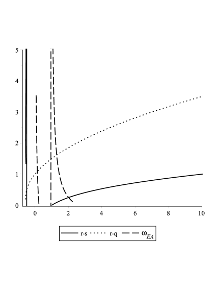
Figure 5: r-s, r-q, $\omega_{Einstein-aether}$ for emergent universe in the redshift $t=\ln\left({{\rm e}^{-{\frac{\ln\left(A+zA\right)}{\lambda}}}}-B\right){n}^{-1}$ range $0.07\leq z\leq 2.3$ with parameters $A=1;B=1;\lambda=2;n=1$.

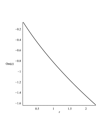
Figure 6: $Om(z)$ for emergent universe in the redshift $t=\ln\left({{\rm e}^{-{\frac{\ln\left(A+zA\right)}{\lambda}}}}-B\right){n}^{-1}$ range $0.07\leq z\leq 2.3$ with parameters $A=1;B=1;\lambda=2;n=1$.

In Figure 8, we plot the first cosmological parameters $r-s$, $r-q$, $\omega_{Einstein-aether}$ for for intermediate inflation, in the redshift $t=\Big{[}-\frac{\ln(1+z)}{B}\Big{]}^{\theta^{-1}}$ range $0.07\leq z\leq 2.3$. A continuous behavior is observed. For $r-s$, we observe that when $r$ is increasing, $s=-1$ remains constant. For $r,q$ when we are increasing $r$, $q$ is decreasing and $-1<q<0$. As we observe, the approved observational value for $q\approx-0.67$ do not exist in this model. In Figure 8, we plot $Om(z)$ for intermediate inflation in the redshift $t=\Big{[}-\frac{\ln(1+z)}{B}\Big{]}^{\theta^{-1}}$ range $0.07\leq z\leq 2.3$. We observe that when the redshift $z$ is increasing within the interval $0.07\leq z\leq 2.3$, the $Om(z)$ is monotonically increasing, and $Om(z)<\Omega_{m0}$, so the intermediate inflation mimics a phantom model with effective EoS $w<-1$.

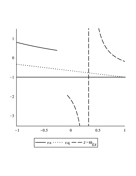
Figure 7: r-s, r-q, $\omega_{Einstein-aether}$ for intermediate inflation in the redshift $t=\Big{[}-\frac{\ln(1+z)}{B}\Big{]}^{\theta^{-1}}$ range $0.07\leq z\leq 2.3$ with parameters $\theta=2;B=1$.

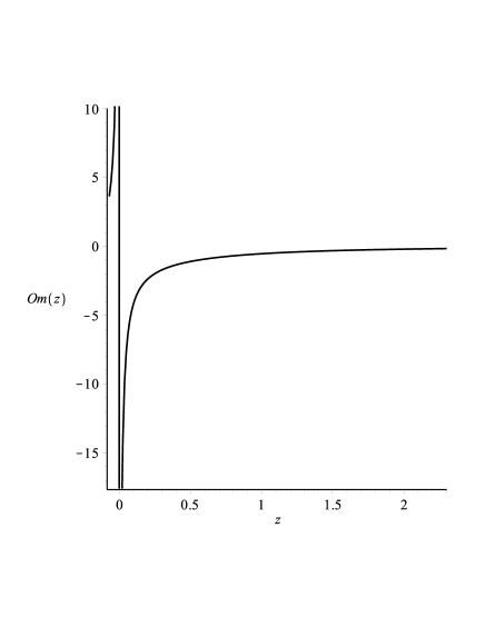
Figure 8: $Om(z)$ for intermediate inflation in the redshift $t=\Big{[}-\frac{\ln(1+z)}{B}\Big{]}^{\theta^{-1}}$ range $0.07\leq z\leq 2.3$ with parameters $\theta=2;B=1$.

6 Observational Constraints

In this section, we will apply observational data from Ia Supernovae Ia, baryonic acoustic oscillations (BAO), and data of the Hubble parameter $H$ to study the constraints on parameters of different cosmological models. The total $\chi^{2}$ for joint data set which we use is defined by

$$\chi_{\rm tot}^{2}=\chi_{\rm SN}^{2}+\chi_{\rm BAO}^{2}+\chi_{\rm Hub}^{2}\,,$$ (6.1)

where the $\chi^{2}_{i}$ for each set of data is evaluated. To compute it we need the luminosity distance $D_{L}(z)$.

Table 1: Values of $\frac{d_{A}(z_{\star})}{D_{V}(Z_{BAO})}$ for distinct values of $z_{BAO}$ [63].

$z_{BAO}$	$\frac{d_{A}(z_{\star})}{D_{V}(Z_{BAO})}$
0.106	$30.95\pm 1.46$
0.2	$17.55\pm 0.60$
0.35	$10.11\pm 0.37$
0.44	$8.44\pm 0.67$
0.6	$6.69\pm 0.33$
0.73	$5.45\pm 0.31$

The luminosity distance is defined as

$$D_{L}(z)=(1+z)\int_{0}^{z}\frac{H_{0}dz^{\prime}}{H(z^{\prime})}.$$ (6.2)

We use the distance modulus $\mu$, which is given by

$$\mu=m-M=5\log D_{L}+\mu_{0},$$ (6.3)

where $m$ and $M$ are defined as the apparent and absolute magnitudes of the Supernovae. Here $\mu_{0}=5\log\left(\frac{H_{0}^{-1}}{\rm Mpc}\right)+25$ is a nuisance parameter (which will be marginalized). We then have that the corresponding $\chi^{2}$ for this data set,

$$\chi_{\rm SN}^{2}(\mu_{0},\theta)=\sum_{i=1}^{580}\frac{\left[\mu_{th}(z_{i},\mu_{0},\theta)-\mu_{obs}(z_{i})\right]^{2}}{\sigma_{\mu}(z_{i})^{2}}\,,$$ (6.4)

where $\mu_{obs}$, $\mu_{th}$ and $\sigma_{\mu}$ indicates the observed distance modulus, the theoretical distance modulus and the uncertainty in the distance modulus, respectively. Furthermore, the parameters in the cosmological models are indicated by $\theta$. For example, for the power law reconstruction scheme it given by $m$, the exponent of in the $q$-de Sitter it is given by the non-extensivity parameter $q$. Now we obtain,

$$\chi_{\rm SN}^{2}(\theta)=A(\theta)-\frac{B(\theta)^{2}}{C(\theta)}\,,$$ (6.5)

where

$$A(\theta)=\sum_{i=1}^{580}\frac{\left[\mu_{th}(z_{i},\mu_{0}=0,\theta)-\mu_{obs}(z_{i})\right]^{2}}{\sigma_{\mu}(z_{i})^{2}}\,,$$ (6.6)

$$B(\theta)=\sum_{i=1}^{580}\frac{\mu_{th}(z_{i},\mu_{0}=0,\theta)-\mu_{obs}(z_{i})}{\sigma_{\mu}(z_{i})^{2}}\,,$$ (6.7)

$$C(\theta)=\sum_{i=1}^{580}\frac{1}{\sigma_{\mu}(z_{i})^{2}}\,.$$ (6.8)

If we use BAO data of $\frac{d_{A}(z_{\star})}{D_{V}(Z_{BAO})}$, we have $z_{\star}\approx 1091$ as the decoupling time, $d_{A}(z)=\int_{0}^{z}\frac{dz^{\prime}}{H(z^{\prime})}$ as the co-moving angular-diameter distance and $D_{V}(z)=\left(d_{A}(z)^{2}\frac{z}{H(z)}\right)^{\frac{1}{3}}$ as the dilation scale. Using this data set, the $\chi_{\mathrm{BAO}}^{2}$ is defined as

$$\chi_{\rm BAO}^{2}=X^{T}C^{-1}X\,.$$ (6.9)

Here what is needed is in the following column vector,

$$X=\left(\begin{array}[]{c}\frac{d_{A}(z_{\star})}{D_{V}(0.106)}-30.95\\ \frac{d_{A}(z_{\star})}{D_{V}(0.2)}-17.55\\ \frac{d_{A}(z_{\star})}{D_{V}(0.35)}-10.11\\ \frac{d_{A}(z_{\star})}{D_{V}(0.44)}-8.44\\ \frac{d_{A}(z_{\star})}{D_{V}(0.6)}-6.69\\ \frac{d_{A}(z_{\star})}{D_{V}(0.73)}-5.45\end{array}\right)\,,$$ (6.10)

Furthermore, the $C^{-1}$ is the inverse covariance matrix. Finally, we use the observational data on Hubble parameter as recently compiled by [63] in the redshift range $0.07\leq z\leq 2.3$. In this data set, the Hubble constant $H_{0}$ is taken from the PLANCK 2013 results [64]. It may be noted that the the normalized Hubble parameter is defined by $h=H/H_{0}$. In this data set, the $\chi^{2}$ for the normalized Hubble parameter is computed as

$$\chi_{\rm Hub}^{2}(\theta)=\sum_{i=1}^{29}\frac{\left[h_{\rm th}(z_{i},\theta)-h_{\rm obs}(z_{i})\right]^{2}}{\sigma_{h}(z_{i})^{2}}\,,$$ (6.11)

where $h_{\rm obs}$ is the observed value of the normalized Hubble parameter, and $h_{\rm th}$ is theoretical values of the normalized Hubble parameter. The error can now be estimated as

$$\sigma_{h}=\left(\frac{\sigma_{H}}{H}+\frac{\sigma_{H_{0}}}{H_{0}}\right)h,$$ (6.12)

where $\sigma_{H}$ is the error in $H$, and $\sigma_{H_{0}}$ is the error in ${H_{0}}$.

Figure 9: This figure shows the $1\sigma$ (plotted in dark) and $2\sigma$ (plotted in light) likelihood contours for different cosmological with joint data (SnIa+Hubble+BAO).

In Figure 9, we plot the $1\sigma$ (dark regions) and $2\sigma$ (light regions) likelihood contours for these cosmological models, Using the joint data (SNIa+Hubble+BAO), we observe that the best fit value of the parameters which are found to be $\Omega_{m0}=0.319$ . Thus, for models with a power-law the best fit occurs for $m=3.218^{+0.0763}_{-0.0564}(1\sigma)\,^{+0.2134}_{-0.0197}(2\sigma)$. Furthermore, it is possible to have analyse certain models with a future singularity after finite time, and for these models, the best fit occurs for $n=4.017^{+0.0765}_{-0.0453}(1\sigma)\,^{+0.2341}_{-0.0876}(2\sigma)$. The best fit for emergent universe occurs for $n=2.054^{+0.0364}_{-0.0312}(1\sigma)\,^{+0.1268}_{-0.0654}(2\sigma),\lambda=6^{+0.0131}_{-0.0976}(1\sigma)\,^{+0.1354}_{-0.0584}(2\sigma)$, and the best fir for intermediate inflation occurs for $B=2.036^{+0.0184}_{-0.0211}(1\sigma)\,^{+0.1287}_{-0.0465}(2\sigma),\theta=0.756^{+0.0123}_{-0.0765}(1\sigma)\,^{+0.1254}_{-0.0512}(2\sigma)$. Thus, we have analysed different cosmological models in Einstein-aether gravity, and used observational data to analyze the value of parameters in these cosmological models.

7 Conclusions

In this paper, we analysed various different cosmological models based on the Einstein-aether gravity. In Einstein-aether gravity, a time-like vector field couples the usual Einstein Lagrangian, and this time-like vector field breaks the Lorentz symmetry of the theory. In this paper, we have analysed various different cosmological models using Einstein-aether gravity. It was demonstrated that the aether field modifies the cosmology in a non-trivial way. Explicit expressions for such a modification to various different cosmological models were derived in this paper. Furthermore, the cosmological models based on Einstein-aether gravity were also compared with observational data. This was done by using the cosmographic analysis involving the Om parametrization. Thus, the SnIa, BAO and Hubble data was used to obtain the $1\sigma$ and $2\sigma$ contours for density parameter $\Omega_{m}$ arising from the Sne Ia $+$ BAO.

It is important to perform such an analysis as it is expected that gravitational waves can be used to test Einstein-aether gravity, and as gravitational wave will be used to test several of the predictions of Einstein-aether gravity, in near future, it is important to analyse the effect of Einstein-aether gravity on cosmology. In fact, it has been predicted that gravitational wave detectors can be used to test Einstein-aether gravity [24]. Thus, it becomes important to analyse various different cosmological models using Einstein-aether gravity. It may be noted that as the Einstein-aether gravity modifies the cosmological models in a non-trivial way, it would also be interesting to analyse quantum cosmology using these modified cosmological models. It would be possible to calculate the Wheeler-DeWitt equation for these cosmological models, and the wave function of the universe can then be obtained as a solution to the Wheeler-DeWitt equation. We would like to mention, that such an analysis would be very interesting and important. Furthermore, as the time-like vector field breaks the time-reparametrization symmetry, it would modify the Wheeler-DeWitt equation in a very non-trivial way. It might be possible to use this time-like aether vector field to obtain a direction of time, even in the Wheeler-DeWitt equation. Thus, it might be possible that this formalism can be used as a solution to the problem of time. It would be interesting to perform such an analysis, for these cosmological models.

It may be noted that the Horava-Lifshitz gravity has been used for analyzing type IIA string theory [75], type IIB string theory [76], AdS/CFT correspondence [77, 78, 79, 80], dilaton black branes [81, 82], and dilaton black holes [83, 84]. As the Horava-Lifshitz gravity is related to the Einstein-aether gravity [20], it would be interesting to analyse these systems using Einstein-aether gravity. In fact, it has been demonstrated that Einstein-aether gravity can be related to the noncritical string [74]. Thus, it would be interesting to analyse this connection further, and also study various cosmological models motivated from string theory in Einstein-aether gravity. It may be noted that the Einstein-aether gravity has been demonstrated to be equivalent to generalization of Horava-Lifshitz gravity

8 Appendix

In this appendix, we will explicitly calculate various cosmological solutions in Einstein-aether gravity.

The first model which we are studying is the power law,

$$a\left(t\right)=a_{0}t^{m}.$$ (8.1)

where $a_{0}$ is the present day value of $a\left(t\right)$, and we must have $m>0$ for an accelerating universe [46]. With the choice of scale factor made in Eq. (8.1), we obtain that the Hubble parameter $H$,

$$H=\frac{\dot{a}\left(t\right)}{a\left(t\right)}=\frac{m}{t}.$$ (8.2)

Moreover, we have that the first and the second time derivatives of the Hubble parameter obtained in Eq. (8.2),

$$\dot{H} = -\frac{m}{t^{2}},$$ (8.3)

$$\ddot{H} = \frac{2m}{t^{3}}.$$ (8.4)

Furthermore, using in Eq. (2.13) the expression of $H$ derived in Eq. (8.2), we obtain that the expression of $K$,

$$K=\frac{3\varepsilon m^{2}}{M^{2}t^{2}}.$$ (8.5)

Using in the general expression of $L_{GO}$ given in Eq. (3.3) the expressions of $H$ and $\dot{H}$ obtained in Eqs. (8.2) and (8.3), we have,

$$L_{GO}=\frac{t}{\sqrt{m(m\alpha-\beta)}}.$$ (8.6)

Therefore, we can conclude that the expression of $\rho_{EA}$ with Granda-Oliveros cut-off can be written as

$$\rho_{EA}=\frac{3c^{2}m(m\alpha-\beta)}{t^{2}}.$$ (8.7)

Using in Eq. (2.21) the expressions of $H$ and $\rho_{EA}$ given in Eqs. (8.2) and (8.7) or equivalently in Eq. (2.22), the expressions of $K$ and $\rho_{EA}$ given in Eqs. (8.5) and (8.7), we obtain the following differential equation for $F\left(K\right)$,

$$\frac{dF\left(K\right)}{dK}-\frac{F\left(K\right)}{2K}-\frac{c^{2}(m\alpha-\beta)}{\varepsilon m}=0,$$ (8.8)

which has the following solution,

$$F\left(K\right)=\frac{2c^{2}K(m\alpha-\beta)}{\varepsilon m}+C_{1}\sqrt{K},$$ (8.9)

where $C_{1}$ represents an integration constant.
Using in Eq. (2.20) the expression of $\rho$ derived in Eq. (8.7) along with the expression of $H$ obtained in Eq. (8.2), we can write the pressure $p_{EA}$ as

$$p_{EA}=\frac{c^{2}\left(2-3m\right)\left(m\alpha-\beta\right)}{t^{2}}.$$ (8.10)

Therefore, the EoS parameter $\omega_{EA}$ is given by

$$\omega_{EA}=\frac{p_{EA}}{\rho_{EA}}=-1+\frac{2}{3m}.$$ (8.11)

At Ricci scale, for $\alpha=2$ and $\beta=1$, we obtain,

$$L_{GO} = \frac{t}{\sqrt{m(2m-1)}},$$ (8.12)

$$\rho_{EA} = \frac{3c^{2}m(2m-1)}{t^{2}},$$ (8.13)

$$F\left(K\right) = \frac{2c^{2}K(2m-1)}{\varepsilon m}+C_{1}\sqrt{K},$$ (8.14)

$$p_{EA} = \frac{c^{2}\left(2-3m\right)\left(2m-1\right)}{t^{2}}.$$ (8.15)

Moreover, for $\alpha\approx 0.8824$ and $\beta\approx 0.5016$, i.e., for the values of $\alpha$ and $\beta$ corresponding to a non-flat Universe, we obtain,

$$L_{GO} = \frac{t}{\sqrt{m(0.8824m-0.5016)}},$$ (8.16)

$$\rho_{EA} = \frac{3c^{2}m(0.8824m-0.5016)}{t^{2}},$$ (8.17)

$$F\left(K\right) = \frac{2c^{2}K(0.8824m-0.5016)}{\varepsilon m}+C_{1}\sqrt{K},$$ (8.18)

$$p_{EA} = \frac{c^{2}\left(2-3m\right)\left(0.8824m-0.5016\right)}{t^{2}}.$$ (8.19)

Furthermore, for $\alpha\approx 0.8502$ and $\beta\approx 0.4817$, i.e., for the values of $\alpha$ and $\beta$ corresponding to a flat Universe, we obtain,

$$L_{GO} = \frac{t}{\sqrt{m(0.8502m-0.4817)}},$$ (8.20)

$$\rho_{EA} = \frac{3c^{2}m(0.8502m-0.4817)}{t^{2}},$$ (8.21)

$$F\left(K\right) = \frac{2c^{2}K(0.8502m-0.4817)}{\varepsilon m}+C_{1}\sqrt{K},$$ (8.22)

$$p_{EA} = \frac{c^{2}\left(2-3m\right)\left(0.8502m-0.4817\right)}{t^{2}}.$$ (8.23)

We now consider the Chen-Jing model studied in this paper, i.e., the one with the first and the second time derivatives of the Hubble parameter $H$. Using the expressions of $H$, $\dot{H}$ and $\ddot{H}$ given in Eqs. (8.2), (8.3) and (8.4) in Eq. (3.7), we obtain the expression of $\rho_{EA}$ with higher derivatives of the Hubble parameter,

$$\rho_{EA}=\frac{3c^{2}\left[2\alpha+m(m\beta-\gamma)\right]}{t^{2}}.$$ (8.24)

Using the expressions of $H$ and $\rho_{EA}$ given in Eqs. (8.2) and (8.24) in Eq. (2.21) or equivalently in Eq. (2.22), the expressions of $K$ and $\rho_{EA}$ from Eqs. (8.5) and (8.24), we obtain the following differential equation for $F\left(K\right)$,

$$\frac{dF\left(K\right)}{dK}-\frac{F\left(K\right)}{2K}-\frac{c^{2}\left[2\alpha+m(m\beta-\gamma)\right]}{\varepsilon m^{2}}=0,$$ (8.25)

whose solution is given by

$$F\left(K\right)=\frac{2c^{2}K\left[2\alpha+m(m\beta-\gamma)\right]}{\varepsilon m^{2}}+C_{2}\sqrt{K},$$ (8.26)

where $C_{2}$ is an integration constant. Substituting in Eq. (2.20) the expression of $\rho_{EA}$ derived in Eq. (8.24), along with the expression of $H$ obtained in Eq. (8.2), we can write the pressure $p_{EA}$ as

$$p_{EA}=-\frac{c^{2}(-2+3m)\left[2\alpha+m\left(m\beta-\gamma\right)\right]}{mt^{2}}.$$ (8.27)

Therefore, the EoS parameter $\omega_{EA}$ is given by

$$\omega_{EA}=\frac{p_{EA}}{\rho_{EA}}=-1+\frac{2}{3m},$$ (8.28)

which is the same as Eq. (8.11).

We now consider the second scale factor considered in this work, which is another form of the power law [51, 52],

$$a\left(t\right)=a_{0}(t_{s}-t)^{-n},$$ (8.29)

where $n>0$ and $t<t_{s}$. Here $a_{0}$ is the present day value of $a(t)$, while $t_{s}$ is the probable future singularity at finite time. So, this model has a future singularity. With the choice of scale factor made in Eq. (8.29), we obtain the Hubble parameter $H$,

$$H=\frac{\dot{a}\left(t\right)}{a\left(t\right)}=\frac{n}{t_{s}-t}.$$ (8.30)

Moreover, the first and the second time derivatives of the Hubble parameter are given by

$$\dot{H} = \frac{n}{(t_{s}-t)^{2}},$$ (8.31)

$$\ddot{H} = \frac{2n}{(t_{s}-t)^{3}}.$$ (8.32)

Furthermore, using in Eq. (2.13) the expression of $H$ derived in Eq. (8.30), we obtain that the expression of $K$,

$$K=\frac{3\varepsilon n^{2}}{M^{2}(t_{s}-t)^{2}}.$$ (8.33)

Using in the general expression of $L_{GO}$ given in Eq. (3.3), the expressions of $H$ and $\dot{H}$ obtained in Eqs. (8.30) and (8.31), we obtain

$$L_{GO}=\frac{\left(t_{s}-t\right)}{\sqrt{n(n\alpha+\beta)}}.$$ (8.34)

Therefore, we can conclude that the expression of $\rho_{EA}$ with Granda-Oliveros cut-off can be written as

$$\rho_{EA}=\frac{3c^{2}n(n\alpha+\beta)}{(t-t_{s})^{2}}.$$ (8.35)

Using in Eq. (2.21) the expressions of $H$ and $\rho_{EA}$ given in Eqs. (8.30) and (8.35), or equivalently in Eq. (2.22) the expressions of $K$ and $\rho_{EA}$ given in Eqs. (8.33) and (8.35), we obtain the following differential equation for $F\left(K\right)$,

$$\frac{dF}{dK}-\frac{F}{2K}-\frac{c^{2}(n\alpha+\beta)}{\varepsilon n}=0,$$ (8.36)

whose solution is given by:

$$F\left(K\right)=\frac{2c^{2}K(n\alpha+\beta)}{\varepsilon n}+C_{3}\sqrt{K},$$ (8.37)

where $C_{3}$ represents an integration constant.

Using in Eq. (2.20) the expression of $\rho_{EA}$ derived in Eq. (8.35), along with the expression of $H$ obtained in Eq. (8.35), we can write the pressure $p_{EA}$ as

$$p_{EA}=\frac{c^{2}\left(2+3n\right)\left(n\alpha+\beta\right)}{\left(t_{s}-t\right)^{2}}.$$ (8.38)

Therefore, the EoS parameter $\omega_{EA}$ is given by

$$\omega_{EA}=\frac{p_{EA}}{\rho_{EA}}=-1-\frac{2}{3n}.$$ (8.39)

At Ricci scale, i.e., for $\alpha=2$ and $\beta=1$, we obtain

$$L_{GO} = \frac{\left(t_{s}-t\right)}{\sqrt{n(2n+1)}},$$ (8.40)

$$\rho_{EA} = \frac{3c^{2}n(2n+1)}{(t-t_{s})^{2}},$$ (8.41)

$$F\left(K\right) = \frac{2c^{2}K(2n+1)}{\varepsilon n}+C_{3}\sqrt{K},$$ (8.42)

$$p_{EA} = \frac{c^{2}\left(2+3n\right)\left(2n+1\right)}{\left(t_{s}-t\right)^{2}}.$$ (8.43)

Moreover, for $\alpha\approx 0.8824$ and $\beta\approx 0.5016$, i.e., for the value of $\alpha$ and $\beta$ corresponding to a non-flat universe, we obtain

$$L_{GO} = \frac{\left(t_{s}-t\right)}{\sqrt{n(0.8824n+0.5016)}},$$ (8.44)

$$\rho_{EA} = \frac{3c^{2}n(0.8824n+0.5016)}{(t-t_{s})^{2}},$$ (8.45)

$$F\left(K\right) = \frac{2c^{2}K(0.8824n+0.5016)}{\varepsilon n}+C_{3}\sqrt{K},$$ (8.46)

$$p_{EA} = \frac{c^{2}\left(2+3n\right)\left(0.8824n+0.5016\right)}{\left(t_{s}-t\right)^{2}}.$$ (8.47)

Furthermore, for $\alpha\approx 0.8502$ and $\beta\approx 0.4817$, i.e., for the value of $\alpha$ and $\beta$ corresponding to a flat Universe, we obtain

$$L_{GO} = \frac{\left(t_{s}-t\right)}{\sqrt{n(0.8502n+0.4817)}},$$ (8.48)

$$\rho_{EA} = \frac{3c^{2}n(0.8502n+0.4817)}{(t-t_{s})^{2}},$$ (8.49)

$$F\left(K\right) = \frac{2c^{2}K(0.8502n+0.4817)}{\varepsilon n}+C_{3}\sqrt{K},$$ (8.50)

$$p_{EA} = \frac{c^{2}\left(2+3n\right)\left(0.8502n+0.4817\right)}{\left(t_{s}-t\right)^{2}}.$$ (8.51)

We now consider the Chen-Jing model studied in this paper, i.e., the energy density model with the first and the second time derivatives of the Hubble parameter $H$. Using in Eq. (3.7) the expressions of $H$, $\dot{H}$ and $\ddot{H}$ obtained in Eqs. (8.30), (8.31) and (8.32), we obtain the expression for $\rho_{EA}$,

$$\rho_{EA}=\frac{3c^{2}}{(t_{s}-t)^{2}}\left[2\alpha+n(n\beta+\gamma)\right].$$ (8.52)

Using in Eq. (2.21) the expressions of $H$ and $\rho_{EA}$ given in Eqs. (8.30) and (8.52), or equivalently in Eq. (2.22) the expressions of $K$ and $\rho_{EA}$ given in Eqs. (8.33) and (8.52), we obtain the following differential equation for $F\left(K\right)$,

$$\frac{dF}{dK}-\frac{F}{2K}-\frac{c^{2}\left[2\alpha+n(n\beta+\gamma)\right]}{\varepsilon n^{2}}=0,$$ (8.53)

which solution is given by,

$$F\left(K\right)=\frac{2c^{2}K\left[2\alpha+n(n\beta+\gamma)\right]}{\varepsilon n^{2}}+C_{4}\sqrt{K},$$ (8.54)

where $C_{4}$ represents an integration constant.

Using in Eq. (2.20) the expression of $\rho_{EA}$ derived in Eq. (8.52) along with the expression of $H$ obtained in Eq. (8.30), we can write the pressure $p_{EA}$ as follows,

$$p_{EA}=-\frac{c^{2}(2+3n)\left[2\alpha+n(n\beta+\gamma)\right]}{n\left(t-t_{s}\right)^{2}}.$$ (8.55)

Therefore, the EoS parameter $\omega_{EA}$ is given by,

$$\omega_{EA}=\frac{p_{EA}}{\rho_{EA}}=-1-\frac{2}{3n},$$ (8.56)

which is the same results of Eq. (8.39).

We can also analyse an emergent universe using this analysis. The scale factor for such a cosmological model is given by [55, 56],

$$a\left(t\right)=A\left(B+e^{nt}\right)^{\lambda}$$ (8.57)

where $A$, $B$, $n$ and $\lambda$ are four positive constant parameters. With the choice of scale factor given in Eq. (8.57), we can obtain the Hubble parameter $H$,

$$H=\frac{e^{nt}n\lambda}{B+e^{nt}}.$$ (8.58)

Moreover, the first and the second time derivatives of the Hubble parameter are given by

$$\dot{H} = \frac{Be^{nt}n^{2}\lambda}{\left(B+e^{nt}\right)^{2}},$$ (8.59)

$$\ddot{H} = \frac{Be^{nt}\left(B-e^{nt}\right)n^{3}\lambda}{\left(B+e^{nt}\right)^{3}}.$$ (8.60)

Furthermore, using in Eq. (2.13) the expression of $H$ derived in Eq. (8.58), we obtain that the expression of $K$

$$K=\frac{3\varepsilon e^{2nt}n^{2}\lambda^{2}}{\left(B+e^{nt}\right)^{2}M^{2}}.$$ (8.61)

Using in the general expression of $L_{GO}$ given in Eq. (3.3) the expressions of $H$ and $\dot{H}$ obtained in Eqs. (8.58) and (8.59), we obtain

$$L_{GO}=\frac{\left(B+e^{nt}\right)}{\sqrt{e^{nt}n^{2}\lambda\left(B\beta+e^{nt}\alpha\lambda\right)}}.$$ (8.62)

Therefore, we can conclude that the expression of $\rho_{EA}$ with Granda-Oliveros cut-off can be written as

$$\rho_{EA}=\frac{3c^{2}e^{nt}n^{2}\lambda\left(B\beta+e^{nt}\alpha\lambda\right)}{\left(B+e^{nt}\right)^{2}}.$$ (8.63)

Using in Eq. (2.21) the expressions of $H$ and $\rho_{EA}$ given in Eqs. (8.58) and (8.63), or equivalently in Eq. (2.22) the expressions of $K$ and $\rho_{EA}$ given in Eqs. (8.61) and (8.63), we obtain the following differential equation for $F\left(K\right)$,

$$\frac{dF}{dK}-\frac{F}{2K}-\frac{c^{2}\left\{\alpha\lambda+\beta\left[-1+\left(\frac{3\varepsilon n^{2}\lambda^{2}}{KM^{2}}\right)^{1/2}\right]\right\}}{\varepsilon\lambda}=0,$$ (8.64)

which has a solution given by

$$F\left(K\right)=\sqrt{K}C_{5}+\frac{c^{2}K\left(2\alpha\lambda-2\beta+\beta\sqrt{\frac{3\varepsilon n^{2}\lambda^{2}}{KM^{2}}}\log K\right)}{\varepsilon\lambda},$$ (8.65)

where $C_{5}$ represents an integration constant.

Using in Eq. (2.20) the expression of $\rho_{EA}$ derived in Eq. (8.63) along with the expression of $H$ obtained in Eq. (8.58), we can write the pressure $p_{EA}$ as

$$p_{EA}=-\frac{c^{2}n^{2}\left\{B^{2}\beta+3e^{2nt}\alpha\lambda^{2}+Be^{nt}\left[2\alpha\lambda+\beta\left(-1+3\lambda\right)\right]\right\}}{\left(B+e^{nt}\right)^{2}}.$$ (8.66)

Therefore, the EoS parameter $\omega_{EA}$ is given by

$$\omega_{EA}=\frac{p_{EA}}{\rho_{EA}}=-1+\frac{B\left(\beta-Be^{-nt}\beta-2\alpha\lambda\right)}{3\lambda\left(B\beta+e^{nt}\alpha\lambda\right)}.$$ (8.67)

At Ricci scale, i.e., for $\alpha=2$ and $\beta=1$, we obtain

$$L_{GO} = \frac{\left(B+e^{nt}\right)}{\sqrt{e^{nt}n^{2}\lambda\left(B+2e^{nt}\lambda\right)}},$$ (8.68)

$$\rho_{EA} = \frac{3c^{2}e^{nt}n^{2}\lambda\left(B+2e^{nt}\lambda\right)}{\left(B+e^{nt}\right)^{2}},$$ (8.69)

$$F\left(K\right) = \sqrt{K}C_{5}+\frac{c^{2}K\left(4\lambda-2+\sqrt{\frac{3\varepsilon n^{2}\lambda^{2}}{KM^{2}}}\log K\right)}{\varepsilon\lambda},$$ (8.70)

$$p_{EA} = -\frac{c^{2}n^{2}\left[B^{2}+6e^{2nt}\lambda^{2}+Be^{nt}(7\lambda-1)\right]}{\left(B+e^{nt}\right)^{2}},$$ (8.71)

$$\omega_{EA} = -1+\frac{B\left(1-Be^{-nt}-4\lambda\right)}{3\lambda\left(B+2e^{nt}\lambda\right)}.$$ (8.72)

For $\alpha\approx 0.8824$ and $\beta\approx 0.5016$, i.e., for the value of $\alpha$ and $\beta$ corresponding to a non-flat Universe, we obtain

$$L_{GO} = \frac{\left(B+e^{nt}\right)}{\sqrt{e^{nt}n^{2}\lambda\left(0.5016B+0.8824e^{nt}\lambda\right)}},$$ (8.73)

$$\rho_{EA} = \frac{3c^{2}e^{nt}n^{2}\lambda\left(0.5016B+0.8824e^{nt}\lambda\right)}{\left(B+e^{nt}\right)^{2}},$$ (8.74)

$$F\left(K\right) = \sqrt{K}C_{5}+\frac{c^{2}K\left(1.7648\lambda-1.0032+0.5016\sqrt{\frac{3\varepsilon n^{2}\lambda^{2}}{KM^{2}}}\log K\right)}{\varepsilon\lambda},$$ (8.75)

$$p_{EA} = -\frac{c^{2}n^{2}\left\{0.5016B^{2}+2.6472e^{2nt}\lambda^{2}+Be^{nt}\left[1.7648\lambda+0.5016\left(-1+3\lambda\right)\right]\right\}}{\left(B+e^{nt}\right)^{2}},$$ (8.76)

$$\omega_{EA} = -1+\frac{B\left(0.5016-0.5016Be^{-nt}-1.7648\lambda\right)}{3\lambda\left(0.5016B+0.8824e^{nt}\lambda\right)}.$$ (8.77)

For $\alpha\approx 0.8502$ and $\beta\approx 0.4817$, i.e., for the value of $\alpha$ and $\beta$ corresponding to a flat Universe, we obtain

$$L_{GO} = \frac{\left(B+e^{nt}\right)}{\sqrt{e^{nt}n^{2}\lambda\left(0.4817B+0.8502e^{nt}\lambda\right)}},$$ (8.78)

$$\rho_{EA} = \frac{3c^{2}e^{nt}n^{2}\lambda\left(0.4817B+0.8502e^{nt}\lambda\right)}{\left(B+e^{nt}\right)^{2}},$$ (8.79)

$$F\left(K\right) = \sqrt{K}C_{5}+\frac{c^{2}K\left(1.7004\lambda-0.9634+0.4817\sqrt{\frac{3\varepsilon n^{2}\lambda^{2}}{KM^{2}}}\log K\right)}{\varepsilon\lambda},$$ (8.80)

$$p_{EA} = -\frac{c^{2}n^{2}\left\{0.4817B^{2}+2.5506e^{2nt}\lambda^{2}+Be^{nt}\left[1.7004\lambda+0.4817\left(-1+3\lambda\right)\right]\right\}}{\left(B+e^{nt}\right)^{2}},$$ (8.81)

$$\omega_{EA} = -1+\frac{B\left(0.4817-0.4817Be^{-nt}-1.7004\lambda\right)}{3\lambda\left(0.4817B+0.8502e^{nt}\lambda\right)}.$$ (8.82)

We now consider the Chen-Jing model studied in this paper, i.e., the energy density model with the first and the second time derivatives of the Hubble parameter $H$. Using in Eq. (3.7) the expressions of $H$, $\dot{H}$ and $\ddot{H}$ obtained in Eqs. (8.58), (8.59) and (8.60), we obtain that the expression of $\rho_{EA}$ is given by

$$\rho_{EA}=\frac{3c^{2}}{\left(B+e^{nt}\right)^{2}}\left[B\left(B-e^{nt}\right)n^{2}\alpha+Be^{nt}n^{2}\gamma\lambda+e^{2nt}n^{2}\beta\lambda^{2}\right].$$ (8.83)

Using in Eq. (2.21) the expressions of $H$ and $\rho_{EA}$ given in Eqs. (8.58) and (8.83), or equivalently in Eq. (2.22) the expressions of $K$ and $\rho_{EA}$ given in Eqs. (8.61) and (8.83), we obtain the following differential equation for $F\left(K\right)$,

$$\frac{dF}{dK} - \frac{F}{2K}-\frac{c^{2}}{3\varepsilon\lambda^{2}}\times$$ (8.84)

$$\left\{\beta\lambda^{2}-\left(\alpha-\gamma\lambda\right)\left[-1+\left(\frac{3\varepsilon n^{2}\lambda^{2}}{KM^{2}}\right)^{1/2}\right]\right.$$

$$\left.+\alpha\left[-1+\left(\frac{3\varepsilon n^{2}\lambda^{2}}{KM^{2}}\right)^{1/2}\right]^{2}\right\}=0,$$

which solution is given by

$$F\left(K\right) = \frac{A_{1}}{B_{1}}+C_{6}\sqrt{K},$$ (8.85)

where $C_{6}$ represents an integration constant, $A_{1}$ and $B_{1}$ are given by

$$A_{1} = c^{2}\left[-6\varepsilon n^{2}\alpha\lambda^{2}+2KM^{2}\left(2\alpha-\gamma\lambda+\beta\lambda^{2}\right)\right.$$ (8.86)

$$\left.+\sqrt{3}KM^{2}\sqrt{\frac{\varepsilon n^{2}\lambda^{2}}{KM^{2}}}\left(-3\alpha+\gamma\lambda\right)\log K\right],$$

$$B_{1} = \varepsilon M^{2}\lambda^{2}.$$ (8.87)

Using in Eq. (2.20) the expression of $\rho_{EA}$ derived in Eq. (8.83) along with the expression of $H$ obtained in Eq. (8.58), we can write the pressure $p_{EA}$ as

$$p_{EA}=\frac{A_{2}}{B_{2}},$$ (8.88)

where

$$A_{2} = c^{2}n^{2}\left\{-3e^{2nt}\beta\lambda^{3}-B^{2}(3\alpha(-1+\lambda)+\gamma\lambda)\right.$$ (8.89)

$$\left.+Be^{nt}\left[\alpha(-1+3\lambda)+\lambda(\gamma-2\beta\lambda-3\gamma\lambda)\right]\right\},$$

$$B_{2} = \left(B+e^{nt}\right)^{2}\lambda.$$ (8.90)

Therefore, the EoS parameter $\omega_{EA}$ is given by

$$\omega_{EA}=\frac{p_{EA}}{\rho_{EA}}=-1+\frac{B\left\{B(3\alpha-\gamma\lambda)-e^{nt}\left[\alpha+\lambda\left(-\gamma+2\beta\lambda\right)\right]\right\}}{3\lambda\left[B^{2}\alpha+e^{2nt}\beta\lambda^{2}+Be^{nt}(-\alpha+\gamma\lambda)\right]}.$$ (8.91)

We now consider the scale factor in the intermediate inflation [53, 54]:

$$a\left(t\right)=e^{Bt^{\theta}},$$ (8.92)

where $B>0$ and $0<\theta<1$. With the choice of scale factor given in Eq. (8.92), we obtain that the Hubble parameter $H$,

$$H=B\theta t^{-1+\theta}.$$ (8.93)

Moreover, we have that the first and the second time derivatives of the Hubble parameter are given by

$$\dot{H} = B(-1+\theta)\theta t^{-2+\theta},$$ (8.94)

$$\ddot{H} = B(-2+\theta)(-1+\theta)\theta t^{-3+\theta}.$$ (8.95)

Furthermore, using in Eq. (2.13) the expression of $H$ derived in Eq. (8.93), we obtain that the expression of $K$

$$K=\frac{3B^{2}\varepsilon t^{-2+2\theta}\theta^{2}}{M^{2}}.$$ (8.96)

Using in the general expression of $L_{GO}$ given in Eq. (3.3), the expressions of $H$ and $\dot{H}$ obtained in Eqs. (8.93) and (8.94), we obtain

$$L_{GO}=\frac{1}{\sqrt{Bt^{-2+\theta}\theta\left[\beta(-1+\theta)+Bt^{\theta}\alpha\theta\right]}}.$$ (8.97)

Therefore, we can conclude that the expression of $\rho_{EA}$ with Granda-Oliveros cut-off can be written as

$$\rho_{EA}=3Bc^{2}t^{-2+\theta}\theta\left[\beta(-1+\theta)+Bt^{\theta}\alpha\theta\right].$$ (8.98)

Using in Eq. (2.21) the expressions of $H$ and $\rho_{EA}$ given in Eqs. (8.92) and (8.98), or equivalently in Eq. (2.22) the expressions of $K$ and $\rho_{EA}$ given in Eqs. (8.96) and (8.98), we obtain the following differential equation for $F\left(K\right)$

$$\frac{dF}{dK}-\frac{F}{2K}-\frac{c^{2}\left[\beta\left(-1+\theta\right)\left(\frac{KM^{2}}{3B^{2}\varepsilon\theta^{2}}\right)^{\frac{-\theta}{2(-1+\theta)}}+B\alpha\theta\right]}{B\varepsilon\theta}=0,$$ (8.99)

which solution is given by

$$F\left(K\right)=\frac{2c^{2}K\left(\frac{KM^{2}}{3B^{2}\varepsilon\theta^{2}}\right)^{\frac{-\theta}{2(-1+\theta)}}\left[-\beta(-1+\theta)^{2}+B\alpha\theta\left(\frac{KM^{2}}{3B^{2}\varepsilon\theta^{2}}\right)^{\frac{\theta}{2(-1+\theta)}}\right]}{B\varepsilon\theta}+C_{7}\sqrt{K},$$ (8.100)

where $C_{7}$ represents an integration constant. Using in Eq. (2.20) the expression of $\rho_{EA}$ derived in Eq. (8.98) along with the expression of $H$ obtained in Eq. (8.93), we can write the pressure $p_{EA}$ as

$$p_{EA}=-\frac{c^{2}\left\{\beta(-1+\theta)\left(-2+\theta+3Bt^{\theta}\theta\right)+Bt^{\theta}\alpha\theta\left[-2+\left(2+3Bt^{\theta}\right)\theta\right]\right\}}{t^{2}}.$$ (8.101)

Therefore, the EoS parameter $\omega_{EA}$ is given by

$$\omega_{EA}=\frac{p_{EA}}{\rho_{EA}}=-1-\frac{t^{-\theta}(-2+\theta)}{3B\theta}+\frac{\alpha\theta}{3\beta-3Bt^{\theta}\alpha\theta-3\beta\theta}.$$ (8.102)

At Ricci scale, i.e., for $\alpha=2$ and $\beta=1$, we obtain

$$L_{GO} = \frac{1}{\sqrt{Bt^{-2+\theta}\theta\left[(-1+\theta)+2Bt^{\theta}\theta\right]}},$$ (8.103)

$$\rho_{EA} = 3Bc^{2}t^{-2+\theta}\theta\left[(-1+\theta)+2Bt^{\theta}\theta\right],$$ (8.104)

$$F\left(K\right) = \frac{2c^{2}K\left(\frac{KM^{2}}{3B^{2}\varepsilon\theta^{2}}\right)^{\frac{-\theta}{2(-1+\theta)}}\left[-(-1+\theta)^{2}+2B\theta\left(\frac{KM^{2}}{3B^{2}\varepsilon\theta^{2}}\right)^{\frac{\theta}{2(-1+\theta)}}\right]}{B\varepsilon\theta}+\sqrt{K}C_{7},$$ (8.105)

$$p_{EA} = -\frac{c^{2}\left\{(-1+\theta)\left(-2+\theta+3Bt^{\theta}\theta\right)+2Bt^{\theta}\theta\left[-2+\left(2+3Bt^{\theta}\right)\theta\right]\right\}}{t^{2}},$$ (8.106)

$$\omega_{EA} = -1-\frac{t^{-\theta}(-2+\theta)}{3B\theta}+\frac{2\theta}{3-6Bt^{\theta}\theta-3\theta}.$$ (8.107)

For $\alpha\approx 0.8824$ and $\beta\approx 0.5016$, i.e., for the value of $\alpha$ and $\beta$ corresponding to a non-flat Universe, we obtain

$$L_{GO} = \frac{1}{\sqrt{Bt^{-2+\theta}\theta\left[0.5016(-1+\theta)+0.8824Bt^{\theta}\theta\right]}},$$ (8.108)

$$\rho_{EA} = 3Bc^{2}t^{-2+\theta}\theta\left[0.5016(-1+\theta)+0.8824Bt^{\theta}\theta\right],$$ (8.109)

$$F\left(K\right) = \frac{2c^{2}K\left(\frac{KM^{2}}{3B^{2}\varepsilon\theta^{2}}\right)^{\frac{-\theta}{2(-1+\theta)}}\left[-0.5016(-1+\theta)^{2}+0.8824B\theta\left(\frac{KM^{2}}{3B^{2}\varepsilon\theta^{2}}\right)^{\frac{\theta}{2(-1+\theta)}}\right]}{B\varepsilon\theta}$$ (8.110)

$$+\sqrt{K}C_{7},$$

$$p_{EA} = -\frac{c^{2}}{t^{2}}\times\left\{0.5016(\theta-1)\left(\theta-2+3Bt^{\theta}\theta\right)\right.$$ (8.111)

$$\left.+0.8824Bt^{\theta}\theta\left[\left(2+3Bt^{\theta}\right)\theta-2\right]\right\},$$

$$\omega_{EA} = -1-\frac{t^{-\theta}(-2+\theta)}{3B\theta}+\frac{0.8824\theta}{1.5048-2.6472Bt^{\theta}\theta-1.5048\theta}.$$ (8.112)

Furthermore, for $\alpha\approx 0.8502$ and $\beta\approx 0.4817$, i.e., for the value of $\alpha$ and $\beta$ corresponding to a flat Universe, we obtain

$$L_{GO} = \frac{1}{\sqrt{Bt^{-2+\theta}\theta\left[0.4817(-1+\theta)+0.8502t^{\theta}\theta\right]}},$$ (8.113)

$$\rho_{EA} = 3Bc^{2}t^{-2+\theta}\theta\left[0.4817(-1+\theta)+0.8502t^{\theta}\theta\right],$$ (8.114)

$$F\left(K\right) = \frac{2c^{2}K\left(\frac{KM^{2}}{3B^{2}\varepsilon\theta^{2}}\right)^{\frac{-\theta}{2(-1+\theta)}}\left[-0.4817(-1+\theta)^{2}+0.8502\theta\left(\frac{KM^{2}}{3B^{2}\varepsilon\theta^{2}}\right)^{\frac{\theta}{2(-1+\theta)}}\right]}{B\varepsilon\theta}$$ (8.115)

$$+\sqrt{K}C_{7},$$

$$p_{EA} = -\frac{c^{2}\left\{0.4817(\theta-1)\left(\theta-2+3Bt^{\theta}\theta\right)+0.8502t^{\theta}\theta\left[\left(2+3Bt^{\theta}\right)\theta-2\right]\right\}}{t^{2}},$$ (8.116)

$$\omega_{EA} = -1-\frac{t^{-\theta}(-2+\theta)}{3B\theta}+\frac{0.8502\theta}{1.5048-2.6472Bt^{\theta}\theta-1.5048\theta}.$$ (8.117)

We now consider the Chen-Jing model studied in this paper, i.e., the one with the first and the second time derivatives of the Hubble parameter $H$. Using in Eq. (3.7) the expressions of $H$, $\dot{H}$ and $\ddot{H}$ obtained in Eqs. (8.93), (8.94) and (8.95), we obtain that the expression of $\rho_{EA}$,

$$\rho_{EA}=3c^{2}\left[\frac{\alpha(-2+\theta)(-1+\theta)}{t^{2}}+Bt^{-2+\theta}\gamma(-1+\theta)\theta+B^{2}t^{-2+2\theta}\beta\theta^{2}\right].$$ (8.118)

Using in Eq. (2.21) the expressions of $H$ and $\rho_{EA}$ given in Eqs. (8.92) and (8.118), or equivalently in Eq. (2.22) the expressions of $K$ and $\rho_{EA}$ given in Eqs. (8.96) and (8.118), we obtain the following differential equation for $F\left(K\right)$,

$$\frac{dF}{dK}-\frac{F}{2K}-\frac{A_{3}}{B_{3}}=0,$$ (8.119)

where

$$A_{3} = 3^{-2^{2\theta}\left(\frac{1}{-1+\theta}\right)^{-2\theta}}c^{2}\left(\frac{KM^{2}}{B^{2}\varepsilon\theta^{2}}\right)^{2^{2\theta}\left(\frac{1}{-1+\theta}\right)^{-2\theta}}\times$$ (8.120)

$$\left\{\alpha(-2+\theta)(-1+\theta)+3^{-2^{-\theta}\left(\frac{1}{-1+\theta}\right)^{\theta}}B\left(\frac{KM^{2}}{B^{2}\varepsilon\theta^{2}}\right)^{2^{-\theta}\left(\frac{1}{-1+\theta}\right)^{\theta}}\theta\times\right.$$

$$\left.\left[\gamma(-1+\theta)+3^{-2^{-\theta}\left(\frac{1}{-1+\theta}\right)^{\theta}}B\beta\left(\frac{KM^{2}}{B^{2}\varepsilon\theta^{2}}\right)^{2^{-\theta}\left(\frac{1}{-1+\theta}\right)^{\theta}}\theta\right]\right\},$$

$$B_{3} = B^{2}\varepsilon\theta^{2}.$$ (8.121)

The solution of Eq. (8.119) is given by

$$F\left(K\right)=\frac{A_{4}}{B_{4}}+C_{8}\sqrt{K},$$ (8.122)

where $C_{8}$ represents an integration constant, and

$$A_{4} = 2\ 3^{-4^{\theta}\left(\frac{1}{-1+\theta}\right)^{-2\theta}-2^{1-\theta}\left(\frac{1}{-1+\theta}\right)^{\theta}}c^{2}K\left(\frac{KM^{2}}{B^{2}\varepsilon\theta^{2}}\right)^{4^{\theta}\left(\frac{1}{-1+\theta}\right)^{-2\theta}}\times$$ (8.123)

$$\left\{\frac{2^{\theta}\beta\left(\frac{1}{-1+\theta}\right)^{2\theta}\left(\frac{KM^{2}}{B^{2}\varepsilon\theta^{2}}\right)^{2^{1-\theta}\left(\frac{1}{-1+\theta}\right)^{\theta}}}{2^{1+3\theta}+2^{\theta}\left(\frac{1}{-1+\theta}\right)^{2\theta}+4\left(\frac{1}{-1+\theta}\right)^{3\theta}}\right.$$

$$\left.+\frac{2^{\theta}3^{2^{-\theta}\left(\frac{1}{-1+\theta}\right)^{\theta}}\gamma\left(\frac{1}{-1+\theta}\right)^{-1+2\theta}\left(\frac{KM^{2}}{B^{2}\varepsilon\theta^{2}}\right)^{2^{-\theta}\left(\frac{1}{-1+\theta}\right)^{\theta}}}{2^{1+3\theta}B\theta+2^{\theta}B\left(\frac{1}{-1+\theta}\right)^{2\theta}\theta+2B\left(\frac{1}{-1+\theta}\right)^{3\theta}\theta}\right.$$

$$\left.+\frac{3^{2^{1-\theta}\left(\frac{1}{-1+\theta}\right)^{\theta}}\alpha\left(2-3\theta+\theta^{2}\right)}{B^{2}\left[1+2^{1+2\theta}\left(\frac{1}{-1+\theta}\right)^{-2\theta}\right]\theta^{2}}\right\},$$

$$B_{4} = \varepsilon.$$ (8.124)

Using in Eq. (2.20) the expression of $\rho_{EA}$ derived in Eq. (8.118) along with the expression of $H$ obtained in Eq. (8.93), we can write the pressure $p_{EA}$ as

$$p_{EA}=-\frac{A_{5}}{B_{5}},$$ (8.125)

where

$$A_{5} = c^{2}t^{-2-\theta}\left\{\alpha(-2+\theta)(-1+\theta)\left(-2+3Bt^{\theta}\theta\right)\right.$$ (8.126)

$$\left.+Bt^{\theta}\theta\left[\gamma(-1+\theta)\left(-2+\theta+3Bt^{\theta}\theta\right)+Bt^{\theta}\beta\theta\left(-2+2\theta+3Bt^{\theta}\theta\right)\right]\right\},$$

$$B_{5} = B\theta.$$ (8.127)

Therefore, the EoS parameter $\omega_{EA}$ is given by

$$\omega_{EA} = \frac{p_{EA}}{\rho_{EA}}=-1+\frac{2t^{-\theta}}{3B\theta}$$ (8.128)

$$-\frac{\theta\left(\gamma(-1+\theta)+2Bt^{\theta}\beta\theta\right)}{3\left\{\alpha(-2+\theta)(-1+\theta)+Bt^{\theta}\theta\left[\gamma\left(-1+\theta\right)+Bt^{\theta}\beta\theta\right]\right\}}.$$

It is possible to analyse matter dominated universe and the accelerated phase of the universe using a single formalism. Now for such a model, the Hubble parameter $H$ is given by [59, 60]

$$H(t)=H_{0}+\frac{H_{1}}{t},$$ (8.129)

with $H_{0}$ and $H_{1}$ being two constant parameters. From Eq. (8.129), we can easily obtain the following expression of the scale factor $a(t)$

$$a(t)=C_{9}e^{H_{0}t}t^{H_{1}},$$ (8.130)

where $C_{9}$ is an integration constant. Moreover, using Eq. (8.129), we have that the first and the second time derivatives of the Hubble parameter, by the following relations:

$$\dot{H} = -\frac{H_{1}}{t^{2}},$$ (8.131)

$$\ddot{H} = \frac{2H_{1}}{t^{3}}.$$ (8.132)

Using in Eq. (2.13) the expression of $H$ given in Eq. (8.129), we obtain the following expression for $K$,

$$K=\frac{3\varepsilon\left(H_{0}+\frac{H_{1}}{t}\right)^{2}}{M^{2}}.$$ (8.133)

Using in the general expression of $L_{GO}$ given in Eq. (3.3), the expressions of $H$ and $\dot{H}$ obtained in Eqs. (8.131) and (8.132), we obtain

$$L_{GO}=\frac{1}{\sqrt{\frac{-\beta H_{1}+\alpha\left(tH_{0}+H_{1}\right)^{2}}{t^{2}}}}=\frac{t}{\sqrt{-\beta H_{1}+\alpha\left(tH_{0}+H_{1}\right)^{2}}}.$$ (8.134)

Therefore, we can conclude that the expression of $\rho_{EA}$ with Granda-Oliveros cut-off can be written as

$$\rho_{EA}=\frac{3c^{2}\left[-\beta H_{1}+\alpha\left(tH_{0}+H_{1}\right)^{2}\right]}{t^{2}}.$$ (8.135)

Using in Eq. (2.21) the expressions of $H$ and $\rho_{EA}$ given in Eqs. (8.131) and (8.135), or equivalently, in Eq. (2.22) the expressions of $K$ and $\rho_{EA}$ given in Eqs. (8.133) and (8.141), we obtain the following differential equation for $F\left(K\right)$

$$\frac{dF}{dK}-\frac{F}{2K}-\frac{3c^{2}\left[\frac{KM^{2}\alpha}{3\varepsilon}-\frac{\beta\left(\frac{1}{3}\varepsilon KM^{2}-H_{0}\right)^{2}}{H_{1}}\right]}{KM^{2}}=0,$$ (8.136)

which solution is given by

$$F\left(K\right) = \sqrt{K}C_{10}$$ (8.137)

$$-\frac{2c^{2}\left[-18\varepsilon^{2}KM^{2}\beta H_{0}-27\varepsilon\beta H_{0}^{2}+KM^{2}\left(\varepsilon^{3}KM^{2}\beta-9\alpha H_{1}\right)\right]}{9\varepsilon M^{2}H_{1}},$$

where $C_{10}$ represents an integration constant.

Using in Eq. (2.20) the expression of $\rho_{EA}$ derived in Eq. (8.135) along with the expression of $H$ defined in Eq. (8.129), we can write the pressure $p_{EA}$ as

$$p_{EA}=\frac{c^{2}\left\{-2\beta H_{1}-\left(tH_{0}+H_{1}\right)\left[3t^{2}\alpha H_{0}^{2}+\left(-2\alpha-3\beta+6t\alpha H_{0}\right)H_{1}+3\alpha H_{1}^{2}\right]\right\}}{t^{2}\left(tH_{0}+H_{1}\right)}.$$ (8.138)

Therefore, we have that the EoS parameter $\omega_{EA}$ for this case is given by

$$\omega_{EA}=-1+\frac{2}{3\left(tH_{0}+H_{1}\right)}-\frac{2t\alpha H_{0}}{3\left[-\beta H_{1}+\alpha\left(tH_{0}+H_{1}\right)^{2}\right]}.$$ (8.139)

At Ricci scale, i.e., for $\alpha=2$ and $\beta=1$, we obtain

$$L_{GO} = \frac{1}{\sqrt{\frac{-H_{1}+2\left(tH_{0}+H_{1}\right)^{2}}{t^{2}}}}=\frac{t}{\sqrt{-H_{1}+2\left(tH_{0}+H_{1}\right)^{2}}},$$ (8.140)

$$\rho_{EA} = \frac{3c^{2}\left[-H_{1}+2\left(tH_{0}+H_{1}\right)^{2}\right]}{t^{2}},$$ (8.141)

$$F(K) = -\frac{2c^{2}\left[-18\varepsilon^{2}KM^{2}H_{0}-27\varepsilon H_{0}^{2}+KM^{2}\left(\varepsilon^{3}KM^{2}-18H_{1}\right)\right]}{9\varepsilon M^{2}H_{1}}$$ (8.142)

$$+\sqrt{K}C_{10},$$

$$p_{EA} = \frac{c^{2}\left\{-2H_{1}-\left(tH_{0}+H_{1}\right)\left[3t^{2}\alpha H_{0}^{2}+\left(-7+12tH_{0}\right)H_{1}+6H_{1}^{2}\right]\right\}}{t^{2}\left(tH_{0}+H_{1}\right)},$$ (8.143)

$$\omega_{EA} = -1+\frac{2}{3\left(tH_{0}+H_{1}\right)}-\frac{4tH_{0}}{3\left[-H_{1}+2\left(tH_{0}+H_{1}\right)^{2}\right]}.$$ (8.144)

For $\alpha\approx 0.8824$ and $\beta\approx 0.5016$, i.e., for the value of $\alpha$ and $\beta$ corresponding to a non-flat universe, we obtain

$$L_{GO} = \frac{1}{\sqrt{\frac{-0.5016H_{1}+0.8824\left(tH_{0}+H_{1}\right)^{2}}{t^{2}}}}=\frac{t}{\sqrt{-0.5016H_{1}+0.8824\left(tH_{0}+H_{1}\right)^{2}}},$$ (8.145)

$$\rho_{EA} = \frac{3c^{2}\left[-0.5016H_{1}+0.8824\left(tH_{0}+H_{1}\right)^{2}\right]}{t^{2}},$$ (8.146)

$$F\left(K\right) = -\frac{2c^{2}\left[-9.0288\varepsilon^{2}KM^{2}H_{0}-13.5431\varepsilon H_{0}^{2}+KM^{2}\left(0.5016\varepsilon^{3}KM^{2}-7.9416H_{1}\right)\right]}{9\varepsilon M^{2}H_{1}}$$ (8.147)

$$+\sqrt{K}C_{10},$$

$$p_{EA} = \frac{c^{2}}{t^{2}\left(tH_{0}+H_{1}\right)}\times\left\{-1.0032H_{1}-\left(tH_{0}+H_{1}\right)\times\right.$$ (8.148)

$$\left.\left[2.6472t^{2}H_{0}^{2}+\left(-3.2696+5.2944tH_{0}\right)H_{1}+2.6472H_{1}^{2}\right]\right\},$$

$$\omega_{EA} = -1+\frac{2}{3\left(tH_{0}+H_{1}\right)}-\frac{1.7648tH_{0}}{3\left[-0.5016H_{1}+0.8824\left(tH_{0}+H_{1}\right)^{2}\right]}.$$ (8.149)

Furthermore, for $\alpha\approx 0.8502$ and $\beta\approx 0.4817$, i.e., for the value of $\alpha$ and $\beta$ corresponding to a flat universe, we obtain

$$L_{GO} = \frac{1}{\sqrt{\frac{-0.4817H_{1}+0.8502\left(tH_{0}+H_{1}\right)^{2}}{t^{2}}}}=\frac{t}{\sqrt{-0.4817H_{1}+0.8502\left(tH_{0}+H_{1}\right)^{2}}},$$ (8.150)

$$\rho_{EA} = \frac{3c^{2}\left[-0.4817H_{1}+0.8502\left(tH_{0}+H_{1}\right)^{2}\right]}{t^{2}},$$ (8.151)

$$F\left(K\right) = -\frac{2c^{2}\left[-8.6706\varepsilon^{2}KM^{2}H_{0}-13.0059\varepsilon H_{0}^{2}+KM^{2}\left(0.4817\varepsilon^{3}KM^{2}-7.5618H_{1}\right)\right]}{9\varepsilon M^{2}H_{1}}$$ (8.152)

$$+\sqrt{K}C_{10},$$

$$p_{EA} = \frac{c^{2}}{t^{2}\left(tH_{0}+H_{1}\right)}\times\left\{-0.9634H_{1}-\left(tH_{0}+H_{1}\right)\times\right.$$ (8.153)

$$\left.\left[2.5506t^{2}H_{0}^{2}+\left(-3.1455+5.1012tH_{0}\right)H_{1}+2.5506H_{1}^{2}\right]\right\},$$

$$\omega_{EA} = -1+\frac{2}{3\left(tH_{0}+H_{1}\right)}-\frac{1.7004tH_{0}}{3\left[-0.4817H_{1}+0.8502\left(tH_{0}+H_{1}\right)^{2}\right]}.$$ (8.154)

We now consider the Chen-Jing model studied in this paper, i.e., the energy density with higher derivatives of the Hubble parameter. Using in Eq. (3.7) the expressions of $H$, $\dot{H}$ and $\ddot{H}$ given in Eqs. (8.129), (8.131) and (8.132), we obtain that the expression of $\rho_{EA}$,

$$\rho_{EA}=\frac{c^{2}\left[-\gamma H_{1}+\frac{2\alpha H_{1}+\beta\left(tH_{0}+H_{1}\right){}^{3}}{tH_{0}+H_{1}}\right]}{3\varepsilon t^{2}\left(H_{0}+\frac{H_{1}}{t}\right)^{2}}.$$ (8.155)

Following the same procedure as in the previous case, we obtain a differential equation for $F\left(K\right)$,

$$F(K) = \sqrt{K}\left[C_{11}+\,{\frac{2{c}^{2}{M}^{2}\alpha\,{K}^{3/2}}{\epsilon\,{H_{{1}}}^{2}}}-{\frac{{c}^{2}{M}^{2}\beta\,{K}^{3/2}}{\epsilon\,H_{{1}}}}+{\frac{{c}^{2}{M}^{2}\gamma\,{K}^{3/2}}{\epsilon}}-\,{\frac{9{c}^{2}\sqrt{2}MH_{{0}}\alpha\,K}{\sqrt{\epsilon}{H_{{1}}}^{2}}}\right.$$ (8.156)

$$\left.+\,{\frac{3{c}^{2}\sqrt{2}MH_{{0}}\beta\,K}{\sqrt{\epsilon}H_{{1}}}}+\,{\frac{18\sqrt{2\epsilon}{c}^{2}{H_{{0}}}^{2}H\alpha\,\ln\left(K\right)}{{H_{{1}}}^{2}M}}-\,{\frac{3\sqrt{2\epsilon}{c}^{2}{H_{{0}}}^{2}H\beta\,\ln\left(K\right)}{H_{{1}}M}}\right.$$

$$\left.-\,{\frac{6\sqrt{2\epsilon}{c}^{2}\alpha\,{H_{{0}}}^{3}\ln\left(K\right)}{{H_{{1}}}^{2}M}}\right],$$

where $C_{11}$ is an integration constant. Using in Eq. (2.20) the expression of $\rho_{EA}$ derived in Eq. (8.155) along with the expression of $H$ obtained in Eq. (8.129), we can write the pressure $p_{EA}$ as

$$p_{EA} = \left\{c^{2}\left[-6\alpha-2\gamma-3t^{2}\beta H_{0}^{2}+\left(2\beta+3\gamma-6t\beta H_{0}\right)H_{1}-\right.\right.$$ (8.157)

$$\left.\left.3\beta H_{1}^{2}-\frac{2t^{2}\alpha H_{0}^{2}}{\left(tH_{0}+H_{1}\right)^{3}}-\frac{2t\alpha H_{0}}{\left(tH_{0}+H_{1}\right){}^{2}}+\frac{4\alpha+2t(3\alpha+\gamma)H_{0}}{tH_{0}+H_{1}}\right]\right\}\times t^{-2}.$$

Therefore, we have that the EoS parameter $\omega_{EA}$ for this case is given by

$$\omega_{EA} = \left\{-6\alpha+2\gamma+3t^{2}\beta H_{0}^{2}+\left(-2\beta-3\gamma+6t\beta H_{0}\right)H_{1}\right.$$ (8.158)

$$\left.+3\beta H_{1}^{2}+\frac{2t^{2}\alpha H_{0}^{2}}{\left(tH_{0}+H_{1}\right){}^{3}}+\frac{2t\alpha H_{0}}{\left(tH_{0}+H_{1}\right){}^{2}}-\frac{2\left[2\alpha+t(3\alpha+\gamma)H_{0}\right]}{tH_{0}+H_{1}}\right\}$$

$$\times\left[3\left(-\gamma H_{1}+\frac{2\alpha H_{1}+\beta\left(tH_{0}+H_{1}\right){}^{3}}{tH_{0}+H_{1}}\right)\right].$$

We can also analyse a $q$-de Sitter model [62]. The scale factor for such a model is given by

$$a(t)=e_{q}(H_{0}t)=\Big{[}1+(q-1)H_{0}t\Big{]}^{\frac{1}{q-1}}.$$ (8.159)

With the choice of scale factor, we can derive that the Hubble parameter $H$ along with its first and second time derivatives are given,

$$H = H_{0}\left[1+H_{0}(-1+q)t\right]^{-1+\frac{1}{-1+q}},$$ (8.160)

$$\dot{H} = H_{0}^{2}\left(-1+\frac{1}{-1+q}\right)(-1+q)\left[1+H_{0}(-1+q)t\right]^{-2+\frac{1}{-1+q}},$$ (8.161)

$$\ddot{H} = H_{0}^{3}\left(-2+\frac{1}{-1+q}\right)\left(-1+\frac{1}{-1+q}\right)\left(-1+q\right)^{2}\times$$ (8.162)

$$\left[1+H_{0}(-1+q)t\right]^{-3+\frac{1}{-1+q}}.$$

Using in Eq. (2.13) the expression of $H$ given in Eq. (8.160), we obtain the following expression for $K$,

$$K=\frac{3\varepsilon H_{0}^{2}[1+H_{0}(-1+q)t]^{-2+\frac{2}{-1+q}}}{M^{2}}.$$ (8.163)

Using in the general expression of $L_{GO}$ given in Eq. (3.3), the expressions of $H$ and $\dot{H}$ obtained in Eqs. (8.160) and (8.161), we obtain

$$L_{GO}=\frac{1}{\sqrt{H_{0}^{2}[1+H_{0}(-1+q)t]^{-2+\frac{1}{-1+q}}\left\{\left[1+H_{0}(-1+q)t\right]^{\frac{1}{-1+q}}\alpha-(-2+q)\beta\right\}}}.$$ (8.164)

Therefore, we conclude that the expression of $\rho_{EA}$ with Granda-Oliveros cut-off can be written as

$$\rho_{EA}=3c^{2}H_{0}^{2}\left[1+H_{0}(-1+q)t\right]^{-2+\frac{1}{-1+q}}\left\{\left[1+H_{0}(-1+q)t\right]^{\frac{1}{-1+q}}\alpha-(-2+q)\beta\right\}.$$ (8.165)

Using in Eq. (2.21) the expressions of $H$ and $\rho_{EA}$ given in Eqs. (8.160) and (8.165), or equivalently, in Eq. (2.22) the expressions of $K$ and $\rho_{EA}$ given in Eqs. (8.163) and (8.165), we a differential equation for $F\left(K\right)$ which solution is given by

$$F(K) = 6c^{2}H_{0}^{2}\left(\frac{K}{\varepsilon H_{0}^{2}}\right)^{1+\frac{1}{-2+q}}\left[\left(\frac{K}{\varepsilon H_{0}^{2}}\right)^{\frac{1}{-2+\frac{2}{-1+q}}}\right]^{\frac{1}{-1+q}}\times$$ (8.166)

$$\left[e^{\frac{q\left((-2+q)\log[K]+\log\left[\frac{K}{\varepsilon H_{0}^{2}}\right]+2(-2+q)\log\left[\left(\frac{K}{\varepsilon H_{0}^{2}}\right)^{-\frac{-1+q}{2(-2+q)}}\right]\right)}{2(-2+q)^{2}(-1+q)}}K^{-\frac{q}{4-6q+2q^{2}}}\times\right.$$

$$\left.\left(\frac{K}{\varepsilon H_{0}^{2}}\right)^{-\frac{-1+2q}{2(-2+q)^{2}(-1+q)}}\alpha-\frac{(-2+q)^{2}\beta}{-1+q}\right]\times M^{-2}+\sqrt{K}C_{12},$$

where $C_{12}$ is a constant parameter.

Using in Eq. (2.20) the expression of $\rho_{EA}$ derived in Eq. (8.165) along with the expression of $H$ defined in Eq. (8.160), we can write the pressure $p_{EA}$ as

$$p_{EA} = \frac{c^{2}H_{0}^{2}}{\left[1+H_{0}(-1+q)t\right]^{2}}\times\left\{-3\left[1+H_{0}(-1+q)t\right]^{\frac{2}{-1+q}}\alpha\right.$$ (8.167)

$$\left.+(-6+(7-2q)q)\beta+(-2+q)\left[1+H_{0}(-1+q)t\right]^{\frac{1}{-1+q}}(2\alpha+3\beta)\right\}.$$

Therefore, the EoS parameter $\omega_{EA}$ for this case is given by

$$\omega_{EA} = \left\{-3\alpha+\left[-6+(7-2q)q\right]\left[1+H_{0}(-1+q)t\right]^{-\frac{2}{-1+q}}\beta\right.$$ (8.168)

$$\left.+(-2+q)\left[1+H_{0}(-1+q)t\right]^{\frac{1}{1-q}}(2\alpha+3\beta)\right\}\times$$

$$\left\{3\alpha-3(-2+q)(1+H_{0}(-1+q)t)^{\frac{1}{1-q}}\beta\right\}^{-1}.$$

At Ricci scale, i.e., for $\alpha=2$ and $\beta=1$, we obtain

$$L_{GO} = \left\{H_{0}^{2}[1+H_{0}\left(-1+q\right)t]^{-2+\frac{1}{-1+q}}\times\right.$$ (8.169)

$$\left.\left\{\left[1+H_{0}(-1+q)t\right]^{\frac{1}{-1+q}}2-(-2+q)\right\}\right\}^{-1/2},$$

$$\rho_{EA} = 3c^{2}H_{0}^{2}\left[1+H_{0}(-1+q)t\right]^{-2+\frac{1}{-1+q}}\times$$ (8.170)

$$\left\{\left[1+H_{0}(-1+q)t\right]^{\frac{1}{-1+q}}2-(-2+q)\right\},$$

$$F\left(K\right) = 6c^{2}H_{0}^{2}\left(\frac{K}{\varepsilon H_{0}^{2}}\right)^{1+\frac{1}{-2+q}}\left[\left(\frac{K}{\varepsilon H_{0}^{2}}\right)^{\frac{1}{-2+\frac{2}{-1+q}}}\right]^{\frac{1}{-1+q}}\times$$ (8.171)

$$\left[e^{\frac{q\left((-2+q)\log[K]+\log\left[\frac{K}{\varepsilon H_{0}^{2}}\right]+2(-2+q)\log\left[\left(\frac{K}{\varepsilon H_{0}^{2}}\right)^{-\frac{-1+q}{2(-2+q)}}\right]\right)}{2(-2+q)^{2}(-1+q)}}K^{-\frac{q}{4-6q+2q^{2}}}\times\right.$$

$$\left.\left(\frac{K}{\varepsilon H_{0}^{2}}\right)^{-\frac{-1+2q}{2(-2+q)^{2}(-1+q)}}2-\frac{(-2+q)^{2}}{-1+q}\right]\times M^{-2}+\sqrt{K}C_{11},$$

$$p_{EA} = \frac{c^{2}H_{0}^{2}}{\left[1+H_{0}(-1+q)t\right]^{2}}\times\left\{-3\left[1+H_{0}(-1+q)t\right]^{\frac{2}{-1+q}}2\right.$$ (8.172)

$$\left.+(-6+(7-2q)q)+(-2+q)\left[1+H_{0}(-1+q)t\right]^{\frac{1}{-1+q}}\cdot 7\right\},$$

$$\omega_{EA} = \left\{-6+\left[-6+(7-2q)q\right]\left[1+H_{0}(-1+q)t\right]^{-\frac{2}{-1+q}}\right.$$ (8.173)

$$\left.+(-2+q)\left[1+H_{0}(-1+q)t\right]^{\frac{1}{1-q}}\cdot 7\right\}\times$$

$$\left\{6-3(-2+q)(1+H_{0}(-1+q)t)^{\frac{1}{1-q}}\right\}^{-1}.$$

For $\alpha\approx 0.8824$ and $\beta\approx 0.5016$, i.e., for the value of $\alpha$ and $\beta$ corresponding to a non-flat universe, we obtain

$$L_{GO} = \left\{H_{0}^{2}[1+H_{0}(-1+q)t]^{-2+\frac{1}{-1+q}}\times\right.$$ (8.174)

$$\left.\left\{\left[1+H_{0}(-1+q)t\right]^{\frac{1}{-1+q}}0.8824-0.5016(-2+q)\right\}\right\}^{-1/2},$$

$$\rho_{EA} = 3c^{2}H_{0}^{2}\left[1+H_{0}(-1+q)t\right]^{-2+\frac{1}{-1+q}}\times$$ (8.175)

$$\left\{\left[1+H_{0}(-1+q)t\right]^{\frac{1}{-1+q}}0.8824-0.5016(-2+q)\right\},$$

$$F(K) = 6c^{2}H_{0}^{2}\left(\frac{K}{\varepsilon H_{0}^{2}}\right)^{1+\frac{1}{-2+q}}\left[\left(\frac{K}{\varepsilon H_{0}^{2}}\right)^{\frac{1}{-2+\frac{2}{-1+q}}}\right]^{\frac{1}{-1+q}}\times$$ (8.176)

$$\left[e^{\frac{q\left((-2+q)\log[K]+\log\left[\frac{K}{\varepsilon H_{0}^{2}}\right]+2(-2+q)\log\left[\left(\frac{K}{\varepsilon H_{0}^{2}}\right)^{-\frac{-1+q}{2(-2+q)}}\right]\right)}{2(-2+q)^{2}(-1+q)}}K^{-\frac{q}{4-6q+2q^{2}}}\times\right.$$

$$\left.\left(\frac{K}{\varepsilon H_{0}^{2}}\right)^{-\frac{-1+2q}{2(-2+q)^{2}(-1+q)}}0.8824-\frac{(-2+q)^{2}\cdot 0.5016}{-1+q}\right]M^{-2}+\sqrt{K}C_{11},$$

$$p_{EA} = \frac{c^{2}H_{0}^{2}}{\left[1+H_{0}(-1+q)t\right]^{2}}\times\left\{-3\left[1+H_{0}(-1+q)t\right]^{\frac{2}{-1+q}}0.8824\right.$$ (8.177)

$$\left.+\left[\left(7-2q\right)q-6\right]\cdot 0.5016+(-2+q)\left[1+H_{0}(-1+q)t\right]^{\frac{1}{-1+q}}\cdot 3.2696\right\},$$

$$\omega_{EA} = \left\{-2.6472+\left[-6+(7-2q)q\right]\left[1+H_{0}(-1+q)t\right]^{-\frac{2}{-1+q}}\cdot 0.5016\right.$$ (8.178)

$$\left.+(-2+q)\left[1+H_{0}(-1+q)t\right]^{\frac{1}{1-q}}\cdot 3.2696\right\}\times$$

$$\left\{2.6472-3(-2+q)(1+H_{0}(-1+q)t)^{\frac{1}{1-q}}\cdot 0.5016\right\}^{-1}.$$

Furthermore, for $\alpha\approx 0.8502$ and $\beta\approx 0.4817$, i.e., for the value of $\alpha$ and $\beta$ corresponding to a flat Universe, we obtain

$$L_{GO} = \left\{H_{0}^{2}[1+H_{0}(-1+q)t]^{-2+\frac{1}{-1+q}}\times\right.$$ (8.179)

$$\left.\left\{\left[1+H_{0}(-1+q)t\right]^{\frac{1}{-1+q}}0.8502-0.4817(-2+q)\right\}\right\}^{-1/2},$$

$$\rho_{EA} = 3c^{2}H_{0}^{2}\left[1+H_{0}(-1+q)t\right]^{-2+\frac{1}{-1+q}}\times$$ (8.180)

$$\left\{\left[1+H_{0}(-1+q)t\right]^{\frac{1}{-1+q}}0.8502-0.4817(-2+q)\right\},$$

$$F(K) = 6c^{2}H_{0}^{2}\left(\frac{K}{\varepsilon H_{0}^{2}}\right)^{1+\frac{1}{-2+q}}\left[\left(\frac{K}{\varepsilon H_{0}^{2}}\right)^{\frac{1}{-2+\frac{2}{-1+q}}}\right]^{\frac{1}{-1+q}}\times$$ (8.181)

$$\left[e^{\frac{q\left((-2+q)\log[K]+\log\left[\frac{K}{\varepsilon H_{0}^{2}}\right]+2(-2+q)\log\left[\left(\frac{K}{\varepsilon H_{0}^{2}}\right)^{-\frac{-1+q}{2(-2+q)}}\right]\right)}{2(-2+q)^{2}(-1+q)}}K^{-\frac{q}{4-6q+2q^{2}}}\times\right.$$

$$\left.\left(\frac{K}{\varepsilon H_{0}^{2}}\right)^{-\frac{-1+2q}{2(-2+q)^{2}(-1+q)}}0.8502-\frac{(-2+q)^{2}\cdot 0.4817}{-1+q}\right]M^{-2}+\sqrt{K}C_{11},$$

$$p_{EA} = \frac{c^{2}H_{0}^{2}}{\left[1+H_{0}(-1+q)t\right]^{2}}\times\left\{-3\left[1+H_{0}(-1+q)t\right]^{\frac{2}{-1+q}}0.8502\right.$$ (8.182)

$$\left.+\left[\left(7-2q\right)q-6\right]\cdot 0.4817+(-2+q)\left[1+H_{0}(-1+q)t\right]^{\frac{1}{-1+q}}\cdot 3.1455\right\},$$

$$\omega_{EA} = \left\{-2.5506+\left[-6+(7-2q)q\right]\left[1+H_{0}(-1+q)t\right]^{-\frac{2}{-1+q}}0.4817\right.$$ (8.183)

$$\left.+(-2+q)\left[1+H_{0}(-1+q)t\right]^{\frac{1}{1-q}}\cdot 3.1455\right\}\times$$

$$\left\{2.5506-3(-2+q)(1+H_{0}(-1+q)t)^{\frac{1}{1-q}}0.4817\right\}^{-1}.$$

We now consider the Chen-Jing model i.e., the one with the first and the second time derivatives of the Hubble parameter $H$. Using in Eq. (3.7) the expressions of $H$, $\dot{H}$ and $\ddot{H}$ obtained in Eqs. (8.160), (8.161) and (8.161), we obtain that the expression of $\rho_{EA}$

$$\rho_{EA} = 3c^{2}H_{0}^{2}\left\{(-2+q)(-3+2q)\alpha+\left[1+H_{0}(-1+q)t\right]^{\frac{1}{-1+q}}\times\right.$$ (8.184)

$$\left.\left[(1+H_{0}(-1+q)t)^{\frac{1}{-1+q}}\beta-(-2+q)\gamma\right]\right\}\times\left[1+H_{0}(-1+q)t\right]^{-2}.$$

Following the same procedure as the previous case, we obtain a differential equation for $F\left(K\right)$ whose solution is given by

$$F(K)=\sqrt{K}C_{13}+\,{\frac{3{c}^{2}\left(2\,\alpha\,{q}^{2}-4\,\alpha\,q+2\,\alpha-\beta\,q+\beta+\gamma\right)}{\epsilon}}K,$$ (8.185)

where $C_{13}$ is a constant of integration.

Using in Eq. (2.20) the expression of $\rho_{EA}$ derived in Eq. (8.184) along with the expression of $H$ obtained in Eq. (8.160), we can write the pressure $p_{EA}$ as

$$p_{EA} = -c^{2}H_{0}^{2}(1+H_{0}(-1+q)t)^{-2+\frac{1}{1-q}}\times$$ (8.186)

$$\left\{-2(-2+q)(-1+q)(-3+2q)\alpha+3\left[1+H_{0}(-1+q)t\right]^{\frac{3}{-1+q}}\beta\right.$$

$$\left.+(-2+q)(-3+2q)\left[1+H_{0}(-1+q)t\right]^{\frac{1}{-1+q}}(3\alpha+\gamma)-\right.$$

$$\left.(-2+q)\left[1+H_{0}(-1+q)t\right]^{\frac{2}{-1+q}}(2\beta+3\gamma)\right\}.$$

Thus, the EoS parameter $\omega_{EA}$ for this case is given by

$$\omega_{EA} = -(1+H_{0}(-1+q)t)^{\frac{1}{1-q}}\times$$ (8.187)

$$\left\{-2(-2+q)(-1+q)(-3+2q)\alpha+3(1+H_{0}(-1+q)t)^{\frac{3}{-1+q}}\beta\right.$$

$$\left.+(-2+q)(-3+2q)(1+H_{0}(-1+q)t)^{\frac{1}{-1+q}}(3\alpha+\gamma)\right.$$

$$\left.-(-2+q)(1+H_{0}(-1+q)t)^{\frac{2}{-1+q}}(2\beta+3\gamma)\right\}$$

$$\times\left\{3\left[(-2+q)(-3+2q)\alpha+\left[1+H_{0}(-1+q)t\right]^{\frac{1}{-1+q}}\times\right.\right.$$

$$\left.\left.\left[(1+H_{0}(-1+q)t)^{\frac{1}{-1+q}}\beta-(-2+q)\gamma\right]\right]\right\}^{-1}.$$

9 Appendix

In this appendix, we provide the $H(z)$ measurements (in unit [$\mathrm{km\,s^{-1}Mpc^{-1}}$]) and their errors [63].

Table 2: $H(z)$ measurements (in unit [$\mathrm{km\,s^{-1}Mpc^{-1}}$]) and their errors [63] .

$z$	$H(z)$	$\sigma_{H}$
0.070	69	19.6
0.100	69	12
0.120	68.6	26.2
0.170	83	8
0.179	75	4
0.199	75	5
0.200	72.9	29.6
0.270	77	14
0.280	88.8	36.6
0.350	76.3	5.6
0.352	83	14
0.400	95	17
0.440	82.6	7.8
0.480	97	62
0.593	104	13
0.600	87.9	6.1
0.680	92	8
0.730	97.3	7.0
0.781	105	12
0.875	125	17
0.880	90	40
0.900	117	23
1.037	154	20
1.300	168	17
1.430	177	18
1.530	140	14
1.750	202	40
2.300	224	8

References

- [1] G. ’t Hooft, Quantization of Point Particles in 2+1 Dimensional Gravity and Space-Time Discreteness, Class. Quantum Gravit. 13, (1996) 1023 [ gr-qc/9601014]
- [2] V. A. Kostelecky and S. Samuel, Spontaneous breaking of Lorentz symmetry in string theory, Phys. Rev. D 39,(1989) 683 [IUHET-139, CCNY-HEP-88/4 ]
- [3] G. Amelino-Camelia, J. R. Ellis, N. Mavromatos, D. V. Nanopoulos and S. Sarkar, Tests of quantum gravity from observations of big gamma-ray bursts, Nature 393,(1998) 763 [astro-ph/9712103]
- [4] R. Gambini and J. Pullin, Nonstandard optics from quantum space-time, Phys. Rev. D 59,(1999) 124021[ gr-qc/9809038].
- [5] M. Faizal, Noncommutativity and Non-Anticommutativity Perturbative Quantum Gravity, Mod. Phys. Lett. A 27, (2012) 1250075 [arXiv:1204.0295].
- [6] S. M. Carroll, J. A. Harvey, V. A. Kostelecky, C. D. Lane and T. Okamoto, Noncommutative Field Theory and Lorentz Violation, Phys. Rev. Lett. 87,(2001) 141601 [ hep-th/0105082].
- [7] M. Faizal, Spontaneous breaking of Lorentz symmetry by ghost condensation in perturbative quantum gravity, J. Phys. A 44, (2011) 402001 [ arXiv:1108.2853].
- [8] K. Greisen,End to the Cosmic-Ray Spectrum?, Phys. Rev. Lett. 16,(1966) 748 [DOI: 10.1103/PhysRevLett.16.748].
- [9] G. T. Zatsepin and V. A. Kuzmin, Upper Limit of the Spectrum of Cosmic Rays, JETP Lett. 4,(1966) 78[Pisma Zh.Eksp.Teor.Fiz. 4 (1966) 114-117].
- [10] J. Abraham et al. (Pierre Auger Collaboration), Measurement of the energy spectrum of cosmic rays above 1018 eV using the Pierre Auger Observatory, Phys. Lett. B 685, (2010) 239[arXiv:1002.197].
- [11] P. Horava, Quantum gravity at a Lifshitz point, Phys. Rev. D 79, 084008 (2009)[ arXiv:0901.3775].
- [12] P. Horava, Spectral dimension of the universe in quantum gravity at a Lifshitz point, Phys. Rev. Lett. 102, (2009) 161301 [arXiv:0902.3657]
- [13] R. G. Cai, B. Hu and H. B. Zhang, Dynamical Scalar Degree of Freedom in Horava-Lifshitz Gravity, Phys. Rev. D 80, (2009) 041501 [arXiv:0905.0255].
- [14] C. Charmousis, G. Niz, A. Padilla and P. M. Saffin, Strong coupling in Horava gravity, JHEP 0908,(2009) 070 [arXiv:0905.2579].
- [15] M. Li and Y. Pang, A trouble with Horava-Lifshitz gravity, JHEP 0908, (2009) 015 [ arXiv:0905.2751].
- [16] T. P. Sotiriou, M. Visser and S. Weinfurtner, Quantum gravity without Lorentz invariance, JHEP 0910,(2009) 033 [arXiv:0905.2798].
- [17] D. Blas, O. Pujolas and S. Sibiryakov, On the Extra Mode and Inconsistency of Horava Gravity, JHEP 0910, (2009) 029 [ arXiv:0906.3046].
- [18] A. A. Kocharyan, Is nonrelativistic gravity possible?, Phys. Rev. D 80, (2009) 024026 [ arXiv:0905.4204].
- [19] D. Blas, O. Pujolas and S. Sibiryakov, Consistent Extension of Horava Gravity, Phys. Rev. Lett. 104,(2010) 181302[ arXiv:0909.3525].
- [20] T. Jacobson, Extended Horava gravity and Einstein-aether theory, Phys. Rev. D81,(2010) 101502[ arXiv:1001.4823 ].
- [21] T. Jacobson, Einstein-aether gravity: a status report, [arXiv:0801.1547]
- [22] K. Yagi, D. Blas, E. Barausse and N. Yunes, Constraints on Einstein-aether theory and Horava gravity from binary pulsar observations, Phys. Rev. D 89,(2014) 084067 [ arXiv:1311.7144].
- [23] C. Heinicke, P. Baekler and F. W. Hehl, Einstein-aether theory, violation of Lorentz invariance, and metric-affine gravity, Phys. Rev. D 72, (2005) 02501 [arXiv:gr-qc/0504005].
- [24] E. Barausse, T. Jacobson and T. P. Sotiriou, Black holes in Einstein-aether and Horava-Lifshitz gravity, Phys. Rev. D 83, (2011) 124043[ arXiv:1104.2889].
- [25] J. D. Barrow, Some inflationary Einstein-Aether cosmologies, Phys. Rev. D 85,(2012) 047503[ arXiv:1201.288].
- [26] H. Wei, X. P. Yan and Y. N. Zhou, Cosmological Evolution of Einstein-Aether Models with Power-law-like Potential, Gen. Rel. Grav. 46, (2014) 1719 [arXiv:1310.533].
- [27] Z. Haghani, T. Harko, H. R. Sepangi and S. Shahidi, Cosmology of a Lorentz violating Galileon theory, JCAP 05,(2015) 022[ arXiv:1501.0081].
- [28] I. D. Saltas, I. Sawicki, L, Amendola and M. Kunz, Anisotropic stress as signature of non-standard propagation of gravitational waves, Phys. Rev. Lett. 113,(2014) 191101[ arXiv:1406.7139].
- [29] T. G Zlosnik, P. G Ferreira and G. D Starkman, Modifying gravity with the aether: An alternative to dark matter, Phys. Rev. D 75, (2007) 044017 [ astro-ph/0607411].
- [30] T. G. Zlosnik, P.G. Ferreira and G. D. Starkman, Growth of structure in theories with a dynamical preferred frame, Phys. Rev. D 77, 084 (2008) 010 [arXiv:0711.0520 ].
- [31] S. Perlmutter, et al., Measurements of Omega and Lambda from 42 High-Redshift Supernovae, Astrophys. J. 517, (1999) 565 [astro-ph/9812133].
- [32] A. G. Riess et al., Observational Evidence from Supernovae for an Accelerating Universe and a Cosmological Constant, Astron. J. 116, (1988) 1009 [ astro-ph/9805201].
- [33] D. N. Spergel et al., [WMAP Collaboration], First-Year Wilkinson Microwave Anisotropy Probe (WMAP) Observations: Determination of Cosmological Parameters, Astrophys. J. Suppl. 148,(2003) 175 [ astro-ph/0302209].
- [34] D. N. Spergel et al., [WMAP Collaboration], Three-Year Wilkinson Microwave Anisotropy Probe (WMAP) Observations: Implications for Cosmology, Astrophys. J. Suppl. 170, (2007) 377 [astro-ph/0603449].
- [35] E. Komatsu et al., Five-year Wilkinson Microwave Anisotropy Probe observations: Cosmological interpretation, Astrophys. J. Suppl. 180, (2009) 330 [ arXiv:0803.0547].
- [36] E. Komatsu et al., [WMAP Collaboration], Seven-year Wilkinson Microwave Anisotropy Probe (WMAP) Observations: Cosmological Interpretation, Astrophys. J. Suppl. 192, (2011) 18 [ arXiv:1001.4538].
- [37] M. Tegmark et al., Cosmological parameters from SDSS and WMAP, Phys. Rev. D 69, (2004) 103501 [ astro-ph/0310723].
- [38] U. Seljak et al., Cosmological parameter analysis including SDSS Lya forest and galaxy bias: Constraints on the primordial spectrum of fluctuations, neutrino mass, and dark energy, Phys. Rev. D 71, (2005) 103515 [ astro-ph/0407372 ].
- [39] D. J. Eisenstein et al., Detection of the Baryon Acoustic Peak in the Large-Scale Correlation Function of SDSS Luminous Red Galaxies, Astrophys. J. 633,(2005) 560 [ astro-ph/0501171].
- [40] B. Jain and A. Taylor, Cross-Correlation Tomography: Measuring Dark Energy Evolution with Weak Lensing, Phys. Rev. Lett. 91, (2003) 141302 [ astro-ph/030604].
- [41] L. N. Granda and A. Oliveros, New infrared cut-off for the holographic scalar fields models of dark energy, Phys. Lett. B, 671,(2009) 199 [ arXiv:0810.3663].
- [42] Y. Wang and L. Xu, Current observational constraints to the holographic dark energy model with a new infrared cutoff via the Markov chain Monte Carlo method, Phys. Rev. D 81, (2010) 083523 [ arXiv:1004.3340].
- [43] S. Chen S, and J. Jing, Dark energy model with higher derivative of Hubble parameter, Phys. Lett. B, 679,(2009) 144 [arXiv:0904.2950 ].
- [44] L. N. Granda and A. Oliveros, Infrared cut-off proposal for the holographic density, Phys. Lett. B, 669,(2008) 275 [arXiv:0810.3149].
- [45] A. Khodam-Mohammadi, Power-Law Entropy Corrected New Holographic Scalar Field Models of Dark Energy with Modified Ir-Cutoff, Mod. Phys. Lett. A 26, (2011) 2487 [arXiv:1107.5455].
- [46] S. Rani, A. Altaibayeva, M. Shahalam, J. K. Singh and R. Myrzakulov, Constraints on cosmological parameters in power-law cosmology, JCAP 1503, 03, (2015) 031 [arXiv:1407.3445].
- [47] P. D. Mannheim, Conformal cosmology with no cosmological constant, Gen. Rel. Grav. 22, (1990) 289.
- [48] Allen R E, (1999), Four testable predictions of instanton cosmology, AIP Conf. Proc. 478, 204 (1999) doi:10.1063/1.59392 [astro-ph/9902042].
- [49] K. Bamba, A. N. Makarenko, A. N. Myagky and S. D. Odintsov, Bouncing cosmology in modified Gauss-Bonnet gravity, Phys. Lett. B 732, (2014) 349 [ arXiv:1403.3242].
- [50] K. Bamba A. N. Makarenko, A. N. Myagky, S. Nojiri and S. D. Odintsov, Bounce cosmology from F(R) gravity and F(R) bigravity, JCAP 01, (2014)008 [ arXiv:1309.3748].
- [51] R. Rangdee and B. Gumjudpai, Tachyonic (phantom) power-law cosmology, Astrophys. Space Science 349,(2014) 975 [arXiv:1210.5550].
- [52] S. Nojiri, S. D. Odintsov and S. Tsujikawa, Properties of singularities in the (phantom) dark energy universe, Phys. Rev. D 71, (2005) 063004 [ hep-th/0501025 ].
- [53] J. D. Barrow and A. R. Liddle, Perturbation spectra from intermediate inflation, Phys. Rev. D47, (1993) 5219 [astro-ph/9303011].
- [54] P. B. Khatua and U. Debnath, Role of chameleon field in accelerating Universe, Astrophys. Space Sci. 326, (2010) 53 [arXiv:1012.1443].
- [55] S. Mukherjee, B. C. Paul, N. K. Dadhich, S. D. Maharaj and A. Beesham, Emergent universe with exotic matter, Class. Quant. Grav. 23, (2006) 6927 [ gr-qc/0605134].
- [56] B. C. Paul and S. Ghose, Emergent universe scenario in the Einstein-Gauss-Bonnet gravity with dilaton, Gen. Rel. Gravit. 42, (2010) 795 [ arXiv:0809.4131].
- [57] F. Darabi, Acceleration of the Universe in Matter Dominant Era by Conformal Symmetry Breaking, Int. J. Theor. Phys. 53, (2014) 881 [arXiv:1305.5378].
- [58] S. Nesseris, S. Basilakos, E. N. Saridakis and L. Perivolaropoulos, Viable f(T) models are practically indistinguishable from CDM, Phys. Rev. D 88,(2013) 103010 [ arXiv:1308.6142].
- [59] S. Nojiri S and S. D. Odintsov, Unifying phantom inflation with late-time acceleration: scalar phantom-non-phantom transition model and generalized holographic dark energy, Gen. Rel. Grav. 38,(2006) 1285 [ hep-th/0506212].
- [60] S. Nojiri and S. D. Odintsov, Accelerating cosmology in modified gravity: from convenient F(R) or string-inspired theory to bimetric F(R) gravity, Int. J. Geom. Meth. Mod. Phys. 11, (2014) 1460006 [arXiv:1306.4426].
- [61] D. A. Lowe, q-deformed de Sitter/conformal field theory correspondence, Phys. Rev. D 70,(2004) 104002 [hep-th/040718].
- [62] M. R. Setare, D. Momeni, V. Kamali and R. Myrzakulov, Inflation driven by q-de Sitter, Int. J. Theor. Phys. 55, (2016)1003 [arXiv:1409.3200].
- [63] O. Farooq and B. Ratra, Hubble Parameter Measurement Constraints on the Cosmological Deceleration-Acceleration Transition Redshift, Astrophys. J. 766, (2013)L7 [ arXiv:1301.5243].
- [64] P. A. R. Ade, et al., Cosmological parameters, [Planck Collaboration] arXiv:1303.5076[astro-ph.CO].
- [65] V. Sahni, T. D. Saini, A. A. Starobinsky and U. Alam, Statefinder: A new geometrical diagnostic of dark energy, Soviet Journal of Experimental and Theoretical Physics Letters, 77,(2003) 201 [astro-ph/0201498].
- [66] U. Alam, V. Sahni, T. D. Saini and A. A. Starobinsky, Exploring the expanding Universe and dark energy using the statefinder diagnostic, Mon. Not. R. Astron. Soc., 344,(2003) 1057 [ astro-ph/0303009].
- [67] Z. G. Huang, X. M. Song, H. Q. Lu and W. Fang W, Statefinder diagnostic for dilaton dark energy, Astrophys. Space Sci. 315,(2008) 175 [arXiv:0802.2320].
- [68] P. Wu and H. Yu H, Observational constraints on f(T) theory, Phys. Lett. B 693,(2010) 415 [arXiv:1006.0674].
- [69] F. Y. Wang, Z. G. Dai and S. Qi, Probing the cosmographic parameters to distinguish between dark energy and modified gravity models, Astron. Astrophys. 507,(2009) 53 [arXiv:0912.5141].
- [70] V. Sahni, A. Shafieloo and A. A. Starobinsky, Two new diagnostics of dark energy, Phys. Rev. D 78,(2008) 103502 [arXiv:0807.3548].
- [71] M. Shahalam, S. Sami S and A. Agarwal, Om diagnostic applied to scalar field models and slowing down of cosmic acceleration, Mon. Not. Roy. Astron. Soc. 448, (2015) 2948 [ arXiv:1501.04047].
- [72] M. Jamil, D. Momeni and R. Myrzakulov, Observational constraints on non-minimally coupled Galileon model, Eur. Phys. J. C 73, (2013) 2347 [arXiv:1302.0129].
- [73] P. de Fromont, C. de Rham, L. Heisenberg and A. Matas, Superluminality in the Bi- and Multi-Galileon, JHEP 1307,(2013) 067 [arXiv:1303.0274].
- [74] W. Westra and S. Zohren, A local induced action for the noncritical string, Class. Quantum Grav. 29,(2012) 095021 [arXiv:1106.1460].
- [75] R. Gregory, S. L. Parameswaran, G. Tasinato and I. Zavala, Lifshitz solutions in supergravity and string theory, JHEP 1012,(2010) 047 [arXiv:1009.3445].
- [76] P. Burda, R. Gregory and S. Ross, Lifshitz flows in IIB and dual field theories, JHEP 1411,(2014) 073 [ arXiv:1408.3271].
- [77] S. S. Gubser and A. Nellore, Ground states of holographic superconductors, Phys.Rev. D 80,(2009) 105007 [arXiv:0908.1972].
- [78] Y. C. Ong and P. Chen, Stability of Horava-Lifshitz black holes in the context of AdS/CFT, Phys. Rev. D 84, (2011) 104044 [arXiv:1106.3555].
- [79] M. Alishahiha and H. Yavartanoo, Conformally Lifshitz solutions from Horava-Lifshitz Gravity, Class. Quant. Grav. 31, (2014) 095008 [arXiv:1212.4190].
- [80] S. Kachru, N. Kundu, A. Saha, R. Samanta and S. P. Trivedi, Interpolating from Bianchi Attractors to Lifshitz and AdS Spacetimes, JHEP 1403,(2014) 074 [ arXiv:1310.574].
- [81] K. Goldstein, N. Iizuka, S. Kachru, S. Prakash, S. P. Trivedi and A. Westphal, Holography of Dyonic Dilaton Black Branes, JHEP 1010, (2010) 027 [ arXiv:1007.2490].
- [82] G. Bertoldi, B. A. Burrington and A. W. Peet, Thermal behavior of charged dilatonic black branes in AdS and UV completions of Lifshitz-like geometries, Phys. Rev. D 82, (2010) 106013 [ arXiv:1007.1464 ].
- [83] M. Kord Zangeneh, A. Sheykhi and M. H. Dehghani, Thermodynamics of topological nonlinear charged Lifshitz black holes, Phys. Rev. D 92, (2015) 024050 [ arXiv:1506.01784].
- [84] J. Tarrio and S. Vandoren, Black holes and black branes in Lifshitz spacetimes, JHEP 1109, (2011) 017 [arXiv:1105.6335].