Finding Perfect Matchings in Bipartite Hypergraphs

Abstract

Haxell’s condition [Hax95] is a natural hypergraph analog of Hall’s condition, which is a well-known necessary and sufficient condition for a bipartite graph to admit a perfect matching. That is, when Haxell’s condition holds it forces the existence of a perfect matching in the bipartite hypergraph. Unlike in graphs, however, there is no known polynomial time algorithm to find the hypergraph perfect matching that is guaranteed to exist when Haxell’s condition is satisfied.

We prove the existence of an efficient algorithm to find perfect matchings in bipartite hypergraphs whenever a stronger version of Haxell’s condition holds. Our algorithm can be seen as a generalization of the classical Hungarian algorithm for finding perfect matchings in bipartite graphs. The techniques we use to achieve this result could be of use more generally in other combinatorial problems on hypergraphs where disjointness structure is crucial, e.g. Set Packing.

Keywords: bipartite hypergraphs, matchings, local search algorithms.

1 Introduction

Bipartite matchings are a ubiquitous quantity across science and engineering. The task of finding a maximum matching (or, specifically, a perfect matching) in a bipartite graph captures a fundamental notion of assignment that has turned out to have wide applicability. One reason their influence has been felt so deeply is essentially computational. The basic fact that maximum matchings in bipartite graphs can be found efficiently is arguably the most important factor in determining their widespread use. Confirming the importance of this problem, decades of research in theoretical computer science has contributed to increasingly faster and more sophisticated algorithms for finding maximum matchings in bipartite graphs. These include connections to other fundamental problems like matrix multiplication [Lov79, MS04]. Most recently, the exciting work of Ma̧dry [Mad13] breaks the decades-old $O(m\sqrt{n})$ Hopcroft-Karp-Karzanov [HK73, Kar73] barrier for finding maximum matchings in bipartite graphs.

In this paper we look at the analogous problem in the hypergraph setting. We address the following question: Do there exist efficient—in the sense of polynomial running time—algorithms to find perfect matchings in bipartite hypergraphs?

In an $r$-uniform bipartite hypergraph the vertex set is partitioned into two sets $A$ and $B$ such that each edge contains exactly one vertex from $A$ and $r-1$ vertices from $B$. A perfect matching is a collection of disjoint edges such that each vertex in $A$ is covered by exactly one edge in the collection.

In order for the question to make any sense at all we need to impose some additional restrictions on the input as any such algorithm that works unconditionally even for the case $r=3$ is tantamount to P$=$NP, as the trivial reduction from $3$-Dimensional Matching shows. In this sense it is not surprising that the question of finding perfect matchings in bipartite hypergraphs was not considered before. However, as we will see, under certain conditions the problem becomes interesting algorithmically. The starting point for such investigations is to ask ourselves if there is a condition similar to Hall’s [Hal35] condition that guarantees the existence of perfect matchings in bipartite hypergraphs. This question was solved in a very satisfying way by Haxell [Hax95] in the mid-90s leading to a striking generalization of Hall’s theorem. The condition is that for every subset $S$ of $A$, the size of the hitting set of hyperedges incident to $S$ must be proportional to the size of $S$. This condition is sufficient to force the existence of a perfect matching in the hypergraph. More formally, given a bipartite hypergraph $H=(A,B,E)$, for a set $S\subseteq A$ let $E_{S}:=\{e\in E\;|\;|e\cap S|=1\}$ be the set of hyperedges of $H$ incident to $S$. For a given collection of edges $F\subseteq E$, define $\tau(F)$ to be the smallest cardinality subset of $B$ that hits all the edges in $F$.

Theorem 1.1 (Haxell [Hax95]).

Let $H=(A,B,E)$ be an $r$-uniform bipartite hypergraph. If

$$\tau(E_{S})>(2r-3)(|S|-1)\quad\forall S\subseteq A,$$

then $H$ admits a perfect matching.

There are several interesting aspects to Theorem 1.1. First, it reduces to Hall’s condition when $r=2$. Second, the statement is “tight” in the sense that it is not true when the strict inequality is replaced by a non-strict one, i.e., for every $r$ there is an $r$-uniform bipartite hypergraph that satisfies Haxell’s condition with non-strict inequalities and yet contains no perfect matching. Finally, in constrast to the graph case, the proof is not constructive and does not lead to an efficient algorithm that also finds the perfect matching.

Besides being interesting objects in their own right, perfect matchings in bipartite hypergraphs have become a crucial concept in recent work [BS06, Fei08, HSS11, AFS12, Sve12, PS12, AKS15] on a particular allocation problem, called Restricted Max-Min Fair Allocation, where the goal is to partition indivisible resources among players in a balanced manner. The latest work that exploits this connection [AKS15] has further shown that local search algorithms based on alternating trees for this problem can be made to run in polynomial time. These developments brought to light the question posed towards the beginning of this section. Is it possible to efficiently find perfect matchings in bipartite hypergraphs by assuming a stronger version of Haxell’s condition?

The question was also raised implicitly by Haeupler, Saha and Srinivasan [HSS11] who write that “Haxell’s theorems are again highly non-constructive ….” As a direction for future research it was therefore asked in [AKS15] if ensuring the much stronger condition

$$\tau(E_{S})\geq 100r|S|\quad\forall S\subseteq A$$ (1)

was sufficient to also find the perfect matching efficiently. The large constant before $r$ reflected the belief that some loss is to be expected, at least by using their techniques. The allocation algorithm underlying their work turned out to yield a weaker guarantee under strengthenings similar to (1). In particular their techniques yield the following theorem.

Theorem 1.2 ([AKS15]).

Let $c>0$ be some absolute constant. Choose any $0<\epsilon\leq 1$, $r\geq 2$ and consider $r$-uniform bipartite hypergraphs $H=(A,B,E)$ that satisfy $\tau(E_{S})\geq(c/\epsilon)\cdot r(|S|-1).$ For such a family of hypergraphs there is a polynomial time algorithm that assigns one hyperedge $e_{a}\in E$ for every vertex $a\in A$ such that it is possible to choose disjoint subsets $\{S_{a}\subseteq e_{a}\cap B\}_{a\in A}$ of cardinality at least $(1-\epsilon)(r-1)$.

Whereas in the allocation setting sufficiently large subsets $\{S_{a}\}_{a\in A}$ also correspond to a good allocation, in a hypergraph setting Theorem 1.2 does not guarantee a collection of valid and disjoint hyperedges unless $\epsilon<1/r$. However, for a choice of $\epsilon$ in latter range, the assumption $\tau(E_{S})\geq(c/\epsilon)\cdot r(|S|-1)$ is much stronger than the one in Theorem 1.1.

Our results

Our main result is that a suitable constructivization of Theorem 1.1 is indeed possible. We prove the following.

Theorem 1.3.

For every fixed choice of $\epsilon>0$ and $r\geq 2$, there exists an algorithm $\mathcal{A}(\epsilon,r)$ that finds, in time polynomial in the size of the input, a perfect matching in $r$-uniform biparite hypergraphs $H=(A,B,E)$ satisfying

$$\tau(E_{S})>(2r-3+\epsilon)(|S|-1)\quad\forall S\subseteq A.$$

Notice that such an algorithm with a polynomial running time dependence on $1/\epsilon$ would be able to efficiently find perfect matchings in bipartite graphs only assuming Haxell’s condition. Currently we see no way of achieving such a result. In particular, our techniques make essential use of the $\epsilon$ strengthening of Haxell’s condition as assumed in Theorem 1.3. We emphasize that the running time of $\mathcal{A}$ depends exponentially on $r$ and $1/\epsilon$, which explains the particular order of the quantifiers in the statement. See also Theorem 5.4 for a slightly stronger corollary of our main result.

An outline of the ideas behind Theorem 1.3 requires setting up some context involving previous work, which we do presently.

Context

It helps to start with the graph case. Here the basic augmenting algorithm (often called the Hungarian algorithm after Kőnig and Egerváry [Wes01]) takes a partial matching and constructs an alternating tree of unmatched and matched edges with an unmatched vertex at the root. For convenience we can imagine this tree partitioned into “layers”, where the $i$th layer contains all vertices at distance $2i-1$ and $2i$ from the root (along with their associated edges in the tree). Matched edges appearing in the tree can also be called “blocking” since they prevent us from augmenting the partial matching immediately. If a leaf of the alternating tree happens to be an unmatched vertex (i.e., the leaf edge is not blocked by some edge in the partial matching) then the corresponding root to leaf path is an augmenting path for the considered matching and thus the augmenting algorithm terminates. The fact that such a leaf always exists is guaranteed by Hall’s condition [Hal35]. The proof of Haxell’s theorem (Theorem 1.1) involves a similar alternating tree, the key difference being that a single hyperedge in the alternating tree may now be blocked by several hyperedges (up to $r-1$) from the partial matching. Therefore, even if a leaf hyperedge in the tree does not intersect any hyperedges from the partial matching, we may not be able to immediately augment the partial matching like in the graph case. What we can do is only swap the corresponding blocking edge (the unique ancestor of the unblocked leaf edge) with the leaf edge in the partial matching and continue. When there are no longer leaf edges in the alternating tree, the existence of a vertex disjoint hyperedge for one of the $A$ vertices in the tree is implied by Haxell’s condition. This alternating tree algorithm for hypergraph matchings by Haxell [Hax95], which underlies Theorem 1.1, is not known to make fewer than exponentially many modifications (swapping operations) to the partial matching before termination (at which point the root is matched).

To make such a local search algorithm efficient [AKS15] devised a similar but different algorithm that ensures a (constant factor) multiplicative increase in the number of blocking edges from layer to layer. This guarantees that the height of the alternating tree is always logarithmic, leading to “short” augmenting paths. They also avoid making changes to the partial matching unless sufficiently many changes can be made at once. In other words, the partial matching is updated lazily. Coupled with other ideas, this leads to a polynomial time combinatorial allocation algorithm that achieves their main result. For the hypergraph setting, however, this only yields Theorem 1.2.

Our Techniques

One obstacle with the algorithm of [AKS15], is that a single blocking edge can block up to $r-1$ hyperedges in the same layer. This effect can accumulate across consecutive layers preventing the desired growth in the number of blocking edges across the layers of the alternating tree, which we require in order to guarantee a logarithmic bound on the height of the alternating tree. This makes it important to view the structure of the blocking edges when the layers of the alternating tree are constructed. On the other hand the problem with the regular alternating tree algorithm for hypergraph matchings [Hax95] is that a single $A$ vertex in a layer can be part of an unbounded number of hyperedges in the next layer in the alternating tree. This skews any subsequent progress made by the alternating tree algorithm vastly in favor of a few $A$ vertices in the previous layers. To avoid this we impose a degree bound on the $A$ vertices in the alternating tree, making the progress more balanced among $A$ vertices in the same layer. In Section 4 we show, despite imposing this upper bound, a multiplicative growth in the number of blocking edges from layer to layer. Next, since the structure of the blocking edges was considered when constructing a layer, this creates complications when we modify the partial matching and some layer in the tree. For example, when some blocking edges are removed by swapping operations in a layer it may be possible to have additional hyperedges for some of the $A$ vertices in the same layer. At this point our algorithm performs a so-called “superposed-build” operation (see Section 3.2) on the layer to check if sufficiently many new hyperedges can be included. If so, it commits the changes, otherwise it ignores the newly available hyperedges.

1.1 Related work

Most relevant to the result of this paper is the line of work concerning alternating tree algorithms for hypergraph matchings starting with the work of Haxell [Hax95]. The algorithmic question of whether the underlying local search algorithm can be made efficient was not considered until the work of Asadpour, Feige and Saberi [AFS12]. They uncovered a beautiful connection to strong integrality gaps for configuration linear programs for allocation problems. This direction was subsequently also pursued by Svensson [Sve12] leading to a breakthrough in the context of scheduling. Both results [AFS12, Sve12] were non-constructive and only proved integrality gap upper bounds. Following these results it became an important question if such approaches based on alternating trees can be turned into efficient algorithms with similar guarantees. Poláček and Svensson [PS12] obtained significant savings leading to a quasipolynomial time alternating tree algorithm for Restricted Max-Min Fair Allocation, but it is still not clear if their approach can be made truly polynomial. Building on these ideas, a polynomial time alternating tree algorithm for the same problem was obtained by Annamalai, Kalaitzis and Svensson [AKS15].

The success of local search for combinatorial problems on hypergraphs where disjointness structure is crucial has been a recurring theme in the literature on $k$-Set Packing [Kar72]. Hurkens and Schrijver [HS89] showed a $(k/2+\epsilon)$ approximation algorithm using an intuitive local search algorithm. Halldórsson [Hal95] then obtained a quasipolynomial $(k+2)/3$-approximation. Using a different approach this was improved by Cygan, Grandoni, and Mastrolilli [CGM13] to a quasipolynomial time $(k+1+\epsilon)/3$-approximation. A polynomial time $(k+2)/3$-approximation was obtained by Sviridenko and Ward [SW13] using color-coding techniques. The best known result for $k$-Set Packing to date is a $(k+1+\epsilon)/3$-approximation due to Cygan [Cyg13], and also by Furer and Yu [FY14]. It is interesting to note that all of these results are based on local search. We believe our techniques to be a useful addition to this repertoire.

In an important direction of research Chan and Lau [CL12] consider the power of linear and semidefinite relaxations for the $k$-Set Packing problem. They show that a particular LP relaxation has integrality gap at most $(k+1)/2$. A different LP relaxation arrived at by applying $O(k^{2})$ rounds of Chvátal-Gomory cuts to the standard LP relaxation was also shown to have no worse integrality gap by Singh and Talwar [ST10]. It remains interesting to consider the applicability of “alternating tree” style analyses, as presented in this paper, to better understand the integrality gaps of such strong LP and SDP relaxations.

For a different notion of bipartiteness in hypergraphs, Conforti et al. [CCKV96] study sufficient conditions for the existence of perfect matchings. We also mention that for the case of general hypergraphs, sufficient conditions in the spirit of Dirac’s theorem for graphs [Dir52] are known (see Alon et al. [AFH⁺12] and references therein).

2 Preliminaries

Definition 2.1 (Bipartite hypergraph).

An $r$-uniform bipartite hypergraph $H=(A,B,E)$ is a hypergraph on a vertex set partitioned into two sets $A$ and $B$ such that for every edge $e\in E$, $|e\cap A|=1$ and $|e\cap B|=r-1$.

Let $H=(A,B,E)$ be a $r$-uniform bipartite hypergraph. It is important to note that we assume that the underlying bipartition of the vertex set is given to the algorithm. We will use $n$ and $m$ to refer to $|A|$ and $|E|$ respectively in $H$. A subset of edges $M\subseteq E$ is called a partial matching if any pair of edges in the set are disjoint. A partial matching whose edges contain every vertex of $A$ is a perfect matching.

We need some notation for referring to the collection of $A$ vertices and $B$ vertices in a set of edges $F\subseteq E$. For a subset of edges $F\subseteq E$ we use $A(F)$ to denote the set $\cup_{e\in F}\;e\cap A.$ $B(F)$ is defined similarly as $\cup_{e\in F}\;e\cap B$.

We say that a vertex $a\in A$ is matched by a partial matching $M$ if $a\in A(M)$. Recall that a perfect matching is a partial matching that matches all the vertices of $A$.

For the definitions that follow consider a fixed partial matching $M$ in $H$. From the context it will always be clear what the considered partial matching is.

Definition 2.2 (Blocking edges).

The set of edges blocking a given edge $e\in E$ is the set

$$\{f\in M\;|\;f\cap e\cap B\not=\emptyset\},$$

i.e., it contains edges in $M$ that prevent us from adding $e$ to it.

Note that $M$ may contain an edge $e^{\prime}$ such that $e^{\prime}\cap e\cap B=\emptyset$ and it matches $\bar{a}$ in $M$, where $\{\bar{a}\}=e\cap A$, in which case we may want to also add $e^{\prime}$ to the set of blocking edges of $e$ but we do not do so according to Definition 2.2.

An edge $e\in E$ is called immediately addable if it has no blocking edges. The name reflects the property that $M\cup\{e\}$ is also a partial matching for such an edge $e$, unless the $A$ vertex contained in $e$ is already matched by $M$. We refer to an edge $e\in E$ as an edge for $a\in A$ if $a\in e$.

The definitions are made with the following simple operation in mind.

Swapping operation

Suppose that $a$ is matched by $M$ through some edge $e\in M$ and that there is an immediately addable edge $f\in E$ for $a$. Then the set $M\setminus\{e\}\cup\{f\}$ is also a partial matching that matches exactly the same set of $A$ vertices as $M$.

A final piece of notation is the following. For a collection of indexed sets $\{S_{0},S_{1},\dots,S_{k}\}$ we write $S_{\leq t}$ to denote

$$\bigcup_{i=0}^{t}S_{i}.$$

Definition 2.3 (Layer).

A layer $L$ for a bipartite hypergraph $H=(A,B,E)$ with respect to a partial matching $M$ is a tuple $(X,Y)$ where

• $X\subseteq E\setminus M$,

• for each pair of distinct edges $e,e^{\prime}\in X$, $e\cap e^{\prime}\cap B=\emptyset$,

• $Y\subseteq M$ is precisely the set of blocking edges of $X$, and

• every $e\in Y$ intersects exactly one edge from $X$.

Definition 2.4 (Alternating tree).

An alternating tree $T$ for a bipartite hypergraph $H=(A,B,E)$ with respect to a partial matching $M$ is a tuple $(L_{0},\dots,L_{\ell})$ such that:

• $L_{0}=(X_{0},Y_{0})$ is defined to be $(\emptyset,\{a_{0}\})$ for some $a_{0}$ not matched by $M$,

• $L_{1},\dots,L_{\ell}$ are layers,

• $A(Y_{i-1})\supseteq A(X_{i})$ for all $i=1,\dots,\ell$, and

• $B(X_{i}\cup Y_{i})\cap B(X_{i^{\prime}}\cup Y_{i^{\prime}})=\emptyset\;\forall i\neq i^{\prime}\in\{0,\dots,\ell\}$.

$a_{0}$ is called the root of the alternating tree $T$. The degree of an $A$ vertex $\bar{a}\in A(Y_{\leq\ell})$ is defined to be the number of edges from $(X_{\leq\ell}\cup Y_{\leq\ell})\setminus Y_{0}$ that contain $\bar{a}$.

Intuition

Our goal will be to obtain an augmenting algorithm that takes some partial matching $M$ that does not match some $a_{0}\in A$ and turns it into a different partial matching $M^{\prime}$ that matches all the vertices of $A(M)\cup\{a_{0}\}$. To accomplish this consider some edge $e\in E$ for $a_{0}$. If it is immediately addable then we are done. Otherwise there are some blocking edges of $e$, call them $F$, that prevent us from adding $e$ to $M$. To make progress we will try to perform a swapping operation on some of the vertices from $A(F)$ thereby reducing the number of blocking edges of $e$. To do so we need to find edges for $A(F)$ which may themselves turn out to be blocked and so on. This alternating structure is captured in our definition of a layer and the tree structure that follows is the reason behind Definition 2.4. See Figure 1 for an example of an alternating tree.

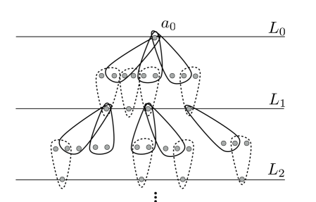
Figure 1: Alternating tree arising from some $3$-uniform bipartite hypergraph and partial matching, depicted here with a root $a_{0}$ and layers $L_{1}$ and $L_{2}$. The edges in $X_{1}$ and $X_{2}$ appear with a solid border, whereas (blocking) edges in $Y_{1}$ and $Y_{2}$ appear with a dotted border. The second edge from the left with a solid border in $L_{2}$ is an example of an immedidately addable edge.

Degree bound

Our augmenting algorithm depends on a single parameter $\mu:=\epsilon^{2}/(10r^{2}).$ We also define $U:=\lceil 1/\mu\rceil.$ As $U+1$ will turn out to be an upper bound on the degree of any $A$ vertex in the alternating tree maintained by the augmenting algorithm, we refer to $U$ as the degree bound. Note that every $A$ vertex in an alternating tree $T$, except for the root, is part of exactly one blocking edge, which follows from Definition 2.4 and the fact that $M$ is a partial matching. Therefore, the degree bound implies that each non-root $A$ vertex can be part of at most $U$ other (non-blocking) edges in the alternating tree.

Remark 2.5.

Without loss of generality we will assume $0<\epsilon<1$. The parameters $\mu,U$ of our augmenting algorithm are set keeping in mind this range of values that $\epsilon$ can assume. If we knew stronger guarantees about the hypergraph $H$, for example, for $\epsilon$ as large as $10r$, then the values of these parameters can be set less aggressively and the running time bounds we obtain in later sections can also be improved drastically. Our goal here, however, is to show the existence of polynomial time algorithms even for a tiny advantage $\epsilon$.

3 The Augmenting Algorithm

3.1 The BuildLayer Subroutine

We first describe a subroutine BuildLayer that is used by the augmenting algorithm. It takes as input an alternating tree $T$, and a pair of sets $X,Y\subseteq E$ that serve as the initial values for the layer that the subroutine constructs. The subroutine augments $X$ and $Y$ and returns them at the end.

$\textbf{BuildLayer}(T,X,Y):$

1. We now describe what we mean by an “addable edge” for some given $X,Y\subseteq E$ and alternating tree $T$. Suppose $T=(L_{0},\dots,L_{\ell})$. For an $A$ vertex $\bar{a}\in A(Y_{\ell})$ we say that $\bar{a}$ has an addable edge if i) $\bar{a}$ has fewer than $U$ edges in $X$, and ii) $\exists$ edge $e\in E$ for $\bar{a}$ disjoint from $B(X_{\leq\ell}\cup Y_{\leq\ell}\cup X\cup Y)$.

2. While there is an $\bar{a}\in A(Y_{\ell})$ having an addable edge $e\in E$, add $e$ to $X$ and its blocking edges to $Y$ as follows:

   $$X \leftarrow X\cup\{e\},$$

   $$Y \leftarrow Y\cup\{f\in M\;|\;f\cap e\cap B\neq\emptyset\}.$$

   EndWhile.

3. Return $(X,Y)$

3.2 Main Algorithm

We now describe the augmenting algorithm. The input to the algorithm is a partial matching $M$ along with an $A$ vertex $a_{0}$ that is not matched by $M$.

Initialization

Initialize layer $L_{0}$ in an alternating tree $T$ by setting $(X_{0},Y_{0})\leftarrow(\emptyset,\{a_{0}\})$. The variable $\ell$ will be updated to always point to the last layer in the tree $T$. Set it to $0$.

Main Loop

Repeat the following two phases in order until $a_{0}$ is matched by $M$.

1. Building phase

   1. Set $(X_{\ell+1},Y_{\ell+1})\leftarrow(\emptyset,\emptyset)$.

   2. $(X_{\ell+1},Y_{\ell+1})\leftarrow\textbf{BuildLayer}(T,X_{\ell+1},Y_{\ell+1}).$

   3. Add the new layer $L_{\ell+1}:=(X_{\ell+1},Y_{\ell+1})$ to $T$.

   4. Increment $\ell$ to $\ell+1$.

2. Collapse phase Recall that $e\in E$ is immediately addable if no edges from $M$ are blocking it, i.e., $f\cap e\cap B=\emptyset\;\forall f\in M$.

   While $X_{\ell}$ contains more than $\mu|X_{\ell}|$ immediately addable edges, perform the following steps:

   For convenience, we call this set of steps in this iteration, the collapse operation of layer $L_{\ell}$.

   1. For each $f\in Y_{\ell-1}$ such that there is an immediately addable edge $e\in X_{\ell}$ for $\bar{a}\in A\cap f$,

      $$M \leftarrow M\setminus\{f\}\cup\{e\},$$

      $$Y_{\ell-1} \leftarrow Y_{\ell-1}\setminus\{f\}.$$

   2. Discard layer $L_{\ell}$ from $T$.

   3. In this step we perform a superposed-build operation on layer $L_{\ell-1}=(X_{\ell-1},Y_{\ell-1})$ in $T$. Note that this layer is modified in this step iff the condition in Step II(c)ii is satisfied.

      1. $(X^{\prime}_{\ell-1},Y^{\prime}_{\ell-1})\leftarrow\textbf{BuildLayer}(T,X_{\ell-1},Y_{\ell-1}).$

      2. If $|X^{\prime}_{\ell-1}|\geq(1+\mu)|X_{\ell-1}|$ then, $(X_{\ell-1},Y_{\ell-1})\leftarrow(X^{\prime}_{\ell-1},Y^{\prime}_{\ell-1})$

   4. $\ell\leftarrow\ell-1$.

   EndWhile.

After the initialization, the main loop of the algorithm consists of repeating the build and collapse phases in order. The state of the algorithm at any moment is described by the alternating tree $T=(L_{0},\dots,L_{\ell})$ and the partial matching $M$ maintained by the algorithm, both of which are dynamically modified. It is not difficult to verify that the addition of an extra layer $L_{\ell+1}$ in the build phase and the collapse operations in the collapse phase modify $T$ and $M$ in legal ways so that the resulting objects are consistent with the definitions of an alternating tree and a partial matching, respectively. We use these facts without mention in the rest of the analayis.

Also note that set of vertices matched by $M$ always remains the same throughout the execution of the algorithm until a collapse operation on layer $L_{1}$ is performed, after which $M$ additionally matches $a_{0}$, and the algorithm terminates.

4 Analysis

We call a layer $L_{i}=(X_{i},Y_{i})$ collapsible if more than $\mu|X_{i}|$ many edges in $X_{i}$ are immediately addable with respect to $M$. This is precisely the condition of the while loop in the collapse phase of the augmenting algorithm from Section 3.2.

Proposition 4.1.

Suppose that the alternating tree $T=(L_{0},\dots,L_{\ell})$ and the partial matching $M$ describe the state at the beginning of some iteration of the main loop of the augmenting algorithm. Then none of the layers $L_{0},\dots,L_{\ell}$ are collapsible. As a corollary it follows that $|Y_{i}|\geq(1-\mu)|X_{i}|$ for each $i=1,\dots,\ell$.

Proof.

Suppose that the statement is true at the beginning of the current iteration. During the build phase a new layer $L_{\ell+1}$ is constructed. If $L_{\ell+1}$ is not collapsible then the claim follows for the beginning of the next iteration since none of the previous layers were modified in the current iteration. If $L_{\ell+1}$ turns out to be collapsible, then by the definition of the collapse phase the layers $L_{0},\dots,L_{t}$ are left at the end of the collapse phase for some $t\leq\ell$ (note that $t\geq 1$ unless $a_{0}$ was matched and the algorithm terminates in the current iteration). The state of each of the layers $L_{0},\dots,L_{t-1}$ is unchanged from the beginning of the current iteration. Layer $L_{t}$ on the other hand could have possibly been modified in Step IIc of the collapse phase. However, since it remains part of the alternating tree after the collapse phase it implies that $L_{t}$, subsequent to any modifications, is not collapsible. Therefore none of the layers in the alternating tree are collapsible at the end of the iteration (unless the algorithm terminates after the current iteration). Since the claim is true for the first iteration, the claim follows by induction on the number of iterations of the main loop of the augmenting algorithm.

The corollary follows since $L_{i}$ is a layer, for each $i=1,\dots,\ell$, and, by Definition 2.3, $Y_{i}$ contains all the blocking edges of edges in $X_{i}$ and each edge in $Y_{i}$ intersects (at most) one edge of $X_{i}$. ∎

Before we state the next proposition some clarification is necessary concerning the description of the augmenting algorithm in Section 3. For instance, in the building phase, there could be many vertices $a\in A(Y_{\ell})$ that have an addable edge (as defined in the Section 3.1), and even a a given vertex could take many addable edges from which one is eventually chosen. The final state of layer $L_{\ell+1}$, at the conclusion of the build phase, depends on the sum total of such choices. The situation is similar in the collapse phase as well. In order to properly specify the algorithm and refer to the quantities maintained by it without ambiguity, we assume that there is a total ordering on the vertices in $A\cup B$ and edges in $E$, and that these orderings are used to choose a unique vertex and edge in any event that many are admissible according to the algorithm description in Section 3. This allows us, for example, to refer precisely to the layer $L_{\ell+1}$ after performing a build operation, or to the layer $L^{\prime}_{\ell}$ after performing a superposed-build operation on layer $L_{\ell}$, etc.

Proposition 4.2.

Suppose that the alternating tree $T=(L_{0},\dots,L_{\ell})$ and the partial matching $M$ describe the state at the beginning of some iteration of the main loop of the augmenting algorithm. Then the superposed-build operation on $L_{i}$ (while ignoring layers $L_{i+1},\dots,L_{\ell}$)

$$(X^{\prime}_{i},Y^{\prime}_{i})\leftarrow\textbf{BuildLayer}((L_{0},\dots,L_{i}),X_{i},Y_{i}),$$

where $L_{i}=(X_{i},Y_{i})$ satisfies $|X^{\prime}_{i}|<(1+\mu)|X_{i}|$ for each $i=1,\dots,\ell$.

Proof.

Consider some layer $L_{t}$ for $0\leq t\leq\ell$ present in the alternating tree at the beginning of the current iteration. At the iteration when layer $L_{t}$ was built a superposed-build operation could not have increased the size of $X_{t}$ even by one. If no collapse operations of some layer occurred until the current iteration then the situation remains identical, because layer $L_{t+1}$ was not collapsed in particular. If however, some layer was collapsed then it must have an index strictly greater than $t$ (since otherwise, the algorithm would have discarded layer $L_{t}$ in that case). As every time layer $L_{t+1}$ is collapsed, and some edges from $Y_{t}$ are removed, the algorithm tries to augment $X_{t}$ by a $\mu$ fraction when possible (in Step IIc of the collapse phase), it follows that the number of edges in $X_{t}$ cannot increase by more than a $\mu$ fraction on performing superposed-build operation on $L_{t}$. ∎

To ensure that the algorithm does not get stuck we need to show that, for some state $(L_{0},\dots,L_{\ell})$ and $M$ reached at the beginning of an iteration of the main loop, the build phase creates a new layer $L_{\ell+1}$ with at least one edge. We prove the following stronger statement.

Theorem 4.3.

Suppose $T=(L_{0},\dots,L_{\ell})$ is the alternating tree at the beginning of some iteration of the main loop of the augmenting algorithm and let $L_{\ell+1}$ be the newly constructed layer in the build phase of the iteration. Then,

$$|X_{i+1}|>\frac{\epsilon}{5r^{2}}|Y_{\leq i}|,$$

for each $i=0,\dots,\ell$.

The proof of Theorem 4.3 uses Lemma 4.4 and Lemma 4.5, which we prove below.

Lemma 4.4.

Suppose that $|Y_{\leq\ell}|<\lceil 5r^{2}/\epsilon\rceil$ at the beginning of some iteration of the main loop. Then when $L_{\ell+1}$ is built in the build phase of the iteration, $|X_{\ell+1}|\geq 1$.

Proof.

By Proposition 4.1, $|X_{\leq\ell}|\leq|Y_{\leq\ell}|/(1-\mu)<6r^{2}/\epsilon,$ where we use that $\mu<1/10$. By the choice of $\mu=\epsilon^{2}/(10r^{2})$ we then have $\mu|X_{\leq\ell}|<1$. Therefore, by the invariants from Proposition 4.1 and Proposition 4.2, every edge in $X_{\leq\ell}$ has at least one blocking edge in the tree, and no $A$ vertex with less than $U$ edges in $X_{\leq\ell}$ has an edge that is disjoint from $B(X_{\leq\ell}\cup Y_{\leq\ell})$. Next, no $A$ vertex in the tree can have $U=\lceil 1/\mu\rceil$ edges in the tree, as in that case the number of blocking edges for that vertex would be at least $U$ which is greater than $\lceil 5r^{2}/\epsilon\rceil$ contradicting our hypothesis. Taking $S$ to be the set of all the $A$ vertices in the tree, so that $|S|=|Y_{\leq\ell}|$, these arguments show that the number of $B$ vertices in the tree is an upper bound on $\tau(E_{S})$.

We now show that the number of $B$ vertices in the tree is at most $(2r-3)(|S|-1)$. To see this, note that every non-root $A$ vertex in the tree is included in a unique edge in $M$ (also in the tree), which in turn intersects some unique edge in $X_{\leq\ell}$. Therefore for each non-root $A$ vertex in the tree, we have $(r-1)$ corresponding $B$ vertices from the matching edge in $M$ and an additional set of at most $(r-1)-1$ many $B$ vertices from the unique edge in the tree that intersects this matching edge. Further, this accounts for all the $B$ vertices in the tree. We may over count some $B$ vertices in edges that were added as addable edges in the alternating tree but this is fine since we are only aiming for an upper bound. So each non-root $A$ vertex can be throught to contribute at most $(r-1)+(r-2)$ many $B$ vertices to the tree.

However, the guarantee is that $\tau(E_{S})$ must be larger than $(2r-3+\epsilon)(|S|-1)$, which is a contradiction. ∎

We can say something stronger than Lemma 4.4 when the number of edges from $M$ in the alternating tree becomes $\Omega(r^{2}/\epsilon)$. Notice that this condition is satisfied when the number of layers in the alternating tree is $\Omega(r^{2}/\epsilon)$.

Lemma 4.5.

If $|Y_{\leq\ell}|\geq\lceil 5r^{2}/\epsilon\rceil$, at the beginning of some iteration then when layer $L_{\ell+1}$ is built

$$|X_{\ell+1}|>\frac{\epsilon}{5r^{2}}|Y_{\leq\ell}|.$$

Proof.

Suppose that after the build phase constructing layer $L_{\ell+1}$ is complete, $|X_{\ell+1}|\leq\delta|Y_{\leq\ell}|$ where $\delta:=\epsilon/(5r^{2})$.

Let $S_{i}$ be the set of $A$ vertices from $A(Y_{i-1})$ that would take an addable edge if we were to perform a superposed-build operation on layer $L_{i}$ while ignoring layers $L_{i+1},\dots,L_{\ell+1}$. Formally, $S_{i}:=A(X^{\prime}_{i}\setminus X_{i}),$ where

$$(X^{\prime}_{i},Y^{\prime}_{i})\leftarrow\textbf{BuildLayer}((L_{0},\dots,L_{i}),X_{i},Y_{i}).$$

Now define $S$ algorithmically (in the sense of performing steps in order) as follows:

• set $S$ to be the set of all $A$ vertices in $Y_{\leq\ell}$,

• remove all $A$ vertices from $S$ that have $U$ edges in the alternating tree (i.e., appear $U$ times in the edges in $X_{\leq\ell+1}$),

• remove all $A$ vertices in $\cup_{i=1}^{\ell}S_{i}$ from $S$.

The number of $A$ vertices that have $U$ edges in the alternating tree is at most $|X_{\leq\ell+1}|/U$. The number of $A$ vertices in $\cup_{i=1}^{\ell}S_{i}$ is upper bounded by $\mu|X_{\leq\ell}|$ using Proposition 4.2. Therefore,

$$|S|\geq|Y_{\leq\ell}|-|X_{\leq\ell+1}|/U-\mu|X_{\leq\ell}|.$$

By our hypothesis towards contradiction $|X_{\ell+1}|\leq\delta|Y_{\leq\ell}|.$ Also, by Proposition 4.1, $|X_{\leq\ell}|\leq|Y_{\leq\ell}|/(1-\mu).$ Putting these together,

$$|S|\geq\left[1-\left(\delta+\frac{1}{1-\mu}\right)\frac{1}{U}-\frac{\mu}{1-\mu}\right]|Y_{\leq\ell}|.$$

As $\tau(E_{S})\geq(2r-3+\epsilon)(|S|-1)$, we have

$$\tau(E_{S})\geq\;(2r-3+\epsilon)\left(\left[1-\left(\delta+\frac{1}{1-\mu}\right)\frac{1}{U}-\frac{\mu}{1-\mu}\right]|Y_{\leq\ell}|-1\right).$$

Recall that $\mu=\epsilon^{2}/(10r^{2})<1/10$. So, after upper bounding the inner sum by

$$\left(\delta+\frac{1}{1-\mu}\right)\frac{1}{U}+\frac{\mu}{1-\mu}\leq\delta\cdot\frac{1}{U}+2\frac{\mu}{1-\mu}<\frac{\epsilon}{5r^{2}}\cdot\frac{\epsilon^{2}}{10r^{2}}+2\cdot\frac{\epsilon^{2}}{10r^{2}}\cdot\frac{10}{9}<\frac{\epsilon^{2}}{2r^{2}},$$

we have

$$\tau(E_{S})>(2r-3+\epsilon)\left(\left[1-\frac{\epsilon^{2}}{2r^{2}}\right]|Y_{\leq\ell}|-1\right).$$ (2)

Next we obtain an upper bound on $\tau(E_{S})$. We start by proving the following claim.

Claim 4.6.

$|B(X_{\leq\ell+1}\cup Y_{\leq\ell+1})|+\mu|X_{\leq\ell}|(r-1)^{2}$ is an upper bound on the cardinality of the smallest size hitting set for $E_{S}$ that is also a subset of $B$, i.e., an upper bound on $\tau(E_{S})$.

Proof.

From the definition of $S$, every vertex $a\in S$ appears in one of the layers $L_{0},\dots,L_{\ell}$ and has strictly less than $U$ edges in the tree. Further, since each $a\in S$ is not part of $\cup_{i=1}^{\ell}S_{i}$ this means that there is no edge in $H$ for the vertex $a$ that is disjoint from the $B$ vertices in the tree and the $B$ vertices introduced in the superposed-build operations in each of the layers $L_{1},\dots,L_{\ell}$. We now bound the total number of such $B$ vertices, to prove the claim.

The number of $B$ vertices present in the alternating tree $T=(L_{0},\dots,L_{\ell+1})$ is simply $|B(X_{\leq\ell+1}\cup Y_{\leq\ell+1})|$. Next, we know by Proposition 4.2 that a superposed-build operation on a layer $L_{i}$ for $1\leq i\leq\ell$ produces a layer $L^{\prime}_{i}$ such that $|X^{\prime}_{i}|<(1+\mu)|X_{i}|$. Further, the set of $B$ vertices introduced in $X^{\prime}_{i}$ (as part of an addable edge and their associated blocking edges) not already present in layer $L_{i}$ (which was counted previously), is at most $\mu|X_{i}|(r-1)^{2}$—each addable edge along with their blocking edges contains at most $(r-1)^{2}$ many $B$ vertices. ∎

We now bound the total number of $B$ vertices in layers $L_{0},\dots,L_{\ell+1}$ in the alternating tree. The contribution from layer $L_{\ell+1}$ is at most $|X_{\ell+1}|(r-1)^{2}$ since each addable edge and its associated set of blocking edges can introduce at most $(r-1)^{2}$ many $B$ vertices. Next, every edge in $X_{\leq\ell}$ is either immediately addable or not. The $B$ vertices in immediately addable edges from layers $L_{0},\dots,L_{\ell}$ is at most $\mu|X_{\leq\ell}|(r-1)$ using Proposition 4.1. The $B$ vertices from layers $L_{0},\dots,L_{\ell}$ that are not present in immediately addable edges can be upper bounded simply by $(|Y_{\leq\ell}|-1)(2r-3)$ using the same argument as in Lemma 4.4.

Therefore, from Claim 4.6 the following upper bound is then obtained for $\tau(E_{s})$:

$$(|Y_{\leq\ell}|-1)(2r-3)+\mu|X_{\leq\ell}|(r-1)+|X_{\ell+1}|(r-1)^{2}+\mu|X_{\leq\ell}|(r-1)^{2}.$$

We now explain the terms in the bound. The first three terms bound the number of $B$ vertices in the alternating tree as we saw above. The final term upper bounds contributions from edges not present in the alternating tree but those that could be added during the superposed-build operations on each of the layers $L_{1},\dots,L_{\ell}$. Using the known bounds on $X_{\leq\ell}\leq Y_{\leq\ell}/(1-\mu)$ (from Proposition 4.1) and $X_{\ell+1}\leq\delta|Y_{\leq\ell}|$ (by hypothesis),

$$\tau(E_{S})<|Y_{\leq\ell}|\left[(2r-3)+\frac{\mu}{1-\mu}\right.(r-1)+\delta(r-1)^{2}+\left.\frac{\mu}{1-\mu}(r-1)^{2}\right].$$

For the chosen parameters $\mu=\epsilon^{2}/(10r^{2})$ and $\delta=\epsilon/(5r^{2})$, we get,

$$\tau(E_{S})<\left[2r-3+\epsilon/2\right]|Y_{\leq\ell}|.$$ (3)

From (2) and (3), we have a contradiction when,

$$\left[2r-3+\epsilon/2\right]|Y_{\leq\ell}|<(2r-3+\epsilon)\left(\left[1-\frac{\epsilon^{2}}{2r^{2}}\right]|Y_{\leq\ell}|-1\right),$$

which is true for $|Y_{\leq\ell}|\geq\lceil 5r^{2}/\epsilon\rceil$. ∎

We now complete the proof of Theorem 4.3.

Proof of Theorem 4.3.

First notice that after a layer $L_{i+1}$ is built, the number of edges in $X_{i+1}$ is non-decreasing until it is collapsed in some future iteration. Also, any collapse operation on a layer leads to discarding that layer. Then the claim follows by combining Lemma 4.4 and Lemma 4.5 to note that at the moment when layer $L_{i+1}$ is created, for some $0\leq i\leq\ell$, the inequality $|X_{i+1}|>\epsilon/(5r^{2})\cdot|Y_{\leq i}|$ holds. This also remains true in future iterations until a collapse operation occurs in layer $L_{i+1}$, in which case it will no longer be part of the alternating tree maintained by the augmenting algorithm. ∎

We are now in a position to bound the number of layers in the alternating tree at any point in the execution of the augmenting algorithm.

Lemma 4.7.

The number of layers in the alternating tree $T=(L_{0},\dots,L_{\ell})$ maintained during the execution of the augmenting algorithm is always bounded by $O(\log n)$.

Proof.

Suppose there are $\ell+1$ layers $L_{0},\dots,L_{\ell}$ at the beginning of some iteration of the main loop of the augmenting algorithm. Consider some layer $L_{i}$ for $1\leq i\leq\ell$. By Proposition 4.1 less than $\mu$ fraction of $X_{i}$ are immediately addable, and hence $|Y_{i}|>(1-\mu)|X_{i}|$. Then by Theorem 4.3 we have

$$|Y_{i}|>\frac{(1-\mu)\epsilon}{(5r^{2})}|Y_{\leq i-1}|$$

for each $i=1,\dots,\ell$. This quickly yields $n=|A|\geq|Y_{\leq\ell}|>(1+(1-\mu)\epsilon/(5r^{2}))^{\ell}|Y_{0}|$, so that $n\geq(1+\gamma)^{\ell}$, where $\gamma:=(1-\mu)\epsilon/(5r^{2})>0$. Altogether this implies that the number of layers $\ell$ at any moment in the algorithm is bounded by $O(\log n)$. ∎

5 Signature Vectors

To keep track of the progress made by the augmenting algorithm we design a potential function. For a given state of the alternating tree with layers $L_{0},\dots,L_{\ell}$ in total we define the signature of layer $L_{i}$ (for $1\leq i\leq\ell$) as:

$$\begin{split}\text{signature}&\text{\;of \;}L_{i}:=\left(-\lfloor\log_{b}\frac{(5r^{2}/\epsilon)^{i}}{(1-\mu)^{i-1}}|X_{i}|\rfloor,\lfloor\log_{b}\frac{(5r^{2}/\epsilon)^{i}}{(1-\mu)^{i}}|Y_{i}|\rfloor\right),\end{split}$$ (4)

where $b:=\frac{1}{1-\mu^{3}}$. The potential function associated with the alternating tree at any state is the sequence obtained by concatenating the signatures of the individual layers in order, and finally appending the symbol $\infty$ at the end. We refer to this potential function as the signature vector. In total there are $2\ell+1$ coordinates in the signature vector which we write as $s=(s_{1},\dots,s_{2\ell},\infty)$.

Lemma 5.1.

The lexicographic value of the signature vector reduces across each iteration of the main loop in the augmenting algorithm unless the algorithm terminates during that iteration.

Proof.

Suppose the alternating tree $T=(L_{0},\dots,L_{\ell})$ and the partial matching $M$ define the state of the algorithm at the beginning of the iteration. Let the signature of the corresponding alternating tree be $s=(s_{1},\dots,s_{2\ell},\infty)$. We consider two cases depending on whether a collapse operation occurred during the collapse phase of the current iteration.

• No collapse operation occurred.   In this case only the build phase of the iteration modified the state of the algorithm by adding a new layer $L_{\ell+1}$. Thus, the new signature of the alternating tree is $s^{\prime}=(s^{\prime}_{1},\dots,s^{\prime}_{2\ell+2},\infty)$ where $s^{\prime}_{i}=s_{i}$ for all $i\leq 2\ell$ and $(s^{\prime}_{2\ell+1},s^{\prime}_{2\ell+2})$ are defined as in (4) for layer $L_{\ell+1}$ at the beginning of the next iteration. Clearly the lexicographic value of the signature of the alternating tree has reduced.

• At least one collapse operation occurred.   This means that during the iteration a new layer $L_{\ell+1}$ was built, and one or more collapse operations occurred in the collapse phase. Let primed quantities denote the variables after the end of the collapse phase in the iteration. Suppose that $t$ ($\leq\ell+1$) is the index of the earliest layer that was collapsed among all the collapse operations in the collapse phase in the iteration. If $t=1$ then $a_{0}$ was matched and the algorithm terminates. Otherwise $t>1$ and by the description of the algorithm, the only layers left in the alternating tree after the collapse phase are $L^{\prime}_{0},\dots,L^{\prime}_{t-1}$ where $L^{\prime}_{i}$ is identical to $L_{i}$ for all $i<t-1$. Thus the new signature after the collapse phase is $s^{\prime}=(s^{\prime}_{1},\dots,s^{\prime}_{2t-2},\infty)$ where $s^{\prime}_{i}=s_{i}$ for all $i\leq 2t-4$ and,

  $$\begin{split}(s^{\prime}_{2t-3},s^{\prime}_{2t-2})=\bigg{(}-\lfloor\log_{b}\frac{(5r^{2}/\epsilon)^{i}}{(1-\mu)^{i-1}}|X^{\prime}_{t-1}|\rfloor,\lfloor\log_{b}\frac{(5r^{2}/\epsilon)^{i}}{(1-\mu)^{i}}|Y^{\prime}_{t-1}|\rfloor\bigg{)}.\end{split}$$

  When layer $L_{t}$ was collapsed Step IIc of the collapse phase could have possibly modified layer $L_{t-1}$. Accordingly there are two subcases.

  • $|X^{\prime}_{t-1}|=|X_{t-1}|.$ Since there was no modification to $X_{t-1}$ we look at how $Y_{t-1}$ has changed. As we collapsed layer $L_{t}$ in the alternating tree, there must have been at least $\mu|X_{t}|$ immediately addable edges in $L_{t}$. These must have caused the removal of at least $\mu|X_{t}|/U$ many matching edges in $L_{t-1}$. Further, by Theorem 4.3, $|X_{t}|>\epsilon/(5r^{2})|Y_{t-1}|$. Together this means that

    $$|Y^{\prime}_{t-1}|<(1-(\mu/U)\cdot\epsilon/(5r^{2}))|Y_{t-1}|<(1-\mu^{3})|Y_{t-1}|.$$

    By our choice of the base of the logarithm it holds that $\log_{b}\frac{(5r^{2}/\epsilon)^{i}}{(1-\mu)^{i}}|Y^{\prime}_{i}|\leq\log_{b}(1-\mu^{3})+\log_{b}\frac{(5r^{2}/\epsilon)^{i}}{(1-\mu)^{i}}|Y_{i}|=-1+\log_{b}\frac{(5r^{2}/\epsilon)^{i}}{(1-\mu)^{i}}|Y_{i}|$. Therefore, $s^{\prime}_{2t-3}=s_{2t-3}$ whereas $s^{\prime}_{2t-2}<s_{2t-2}$.

  • $|X^{\prime}_{t-1}|\geq(1+\mu)|X_{t-1}|.$ In this subcase the fact that $(1+\mu)\geq b$ implies that the lexicographic value of the signature vector has reduced since $s^{\prime}_{2t-3}<s_{2t-3}$.

∎

To show that the augmenting algorithm terminates in polynomial time we need one more fact.

Proposition 5.2.

The coordinates of the signature vector are non-decreasing in absolute value at the beginning of each iteration of the main loop of the augmenting algorithm.

Proof.

Consider some layer $L_{i}$ for $1\leq i\leq\ell$. Clearly the corresponding pair of coordinates $s_{2i-1},s_{2i}$ in the signature vector are non-decreasing in absolute value since $|Y_{i}|\geq(1-\mu)|X_{i}|$ using Proposition 4.1. Between any two layers, by Theorem 4.3 we have $|X_{i}|>\epsilon/(5r^{2})|Y_{i-1}|$ and so $|s_{2i-2}|\leq|s_{2i-1}|$. Thus the coordinates are non-decreasing in absolute value in the signature vector. ∎

Lemma 5.3.

The number of signature vectors is bounded by a polynomial in $n$.

Proof.

By Lemma 4.7 we know that the signature vector has at most $O(\log n)$ coordinates. By Proposition 5.2 the coordinates are also integers that are non-decreasing in absolute value. At this point one can obtain a trivial bound of $O(\log n)$ on the absolute value of each coordinate of the signature vector using the definition in (4) and Lemma 4.7. Since the sign pattern of the signature vector is always fixed, each signature vector can be thought to describe a unique partition of some positive integer of size at most $O(\log^{2}n)$. Recall that a partition of a positive integer $N$ is a way of writing $N$ as the sum of positive integers without regard to order. Since the number of partitions of an integer of size $t$ is (asymptotically) at most $c^{\sqrt{t}}$ for some absolute constant $c>1$ [HR18], the claim then follows. ∎

As noticed by one of the reviewers, the dependence of Lemma 5.3 on the asymptotics of the partition function can be avoided by modifying the signature vector to ensure that its entries are strictly increasing in absolute value (instead of simply being non-decreasing as in Lemma 5.2), thereby allowing a signature vector to be inferred by specifying a subset of a set of size at most $O(\log n)$. One way to get this property is by adding/subtracting $i$ to the $i$-th coordinate of the signature vector, consistent with its sign pattern.

We are now in a position to use the potential function defined in this section to wrap up the proof of our main result.

Proof of Theorem 1.3.

From Lemma 5.1 we have that every iteration of the main loop of the augmenting algorithm described in Section 3 reduces the lexicographic value of the signature vector. Lemma 5.3 further tells us that the number of such signature vectors is bounded by a polynomial in $n$. Thus, the augmenting algorithm terminates in polynomially many iterations. It can also be verified that each iteration of the augmenting algorithm can be implemented to run in time polynomial in $n$ and $m$. Finally, running the augmenting algorithm $n$ times, starting with an empty partial matching, yields the desired perfect matching in $H$. ∎

From the proof of Lemma 4.5 we also note that the algorithm in Section 3 can be suitably modified to yield the following slightly stronger version of Theorem 1.3 as a corollary.

Theorem 5.4.

For every fixed choice of $\epsilon>0$ and $r\geq 2$, there exists an algorithm $\mathcal{A}^{\prime}(\epsilon,r)$ that takes as input an $r$-uniform bipartite hypergraph $H=(A,B,E)$, runs in polynomial time, and terminates after finding either:

• a perfect matching in $H$, or

• a set $S\subseteq A$ such that $\tau(E_{S})\leq(2r-3+\epsilon)(|S|-1).$

6 Conclusion and Open Problems

In this paper we presented a polynomial time algorithm for finding perfect matchings in bipartite hypergraphs satisfying a slightly stronger version of Haxell’s condition. The algorithm is essentially the natural generalization of the well known Hungarian algorithm for finding perfect matchings in graphs with two essential modifications: i) restricting the degree of vertices in the constructed alternating tree, and ii) performing updates on the alternating tree lazily. The two ideas in tandem give us a polynomial running time bound on the procedure.

One subtlety here is that the algorithm performs lazy updates in two places, in Steps IIa and IIc, in the collapse phase. While the former is crucial for the running time bound, the latter seems to be an artifact of the analysis driven by the specific choice of the signature vector in Section 4. In particular, this can likely be avoided by choosing a different signature vector to measure progress.

Finally, we point out the obvious open problem in this line of work.

Question 6.1.

Does there exist such an algorithm with a polynomial running time dependence on at least one of the parameters $1/\epsilon$ and $r$?

References

- [AFH+12] Noga Alon, Peter Frankl, Hao Huang, Vojtech Rödl, Andrzej Ruciński, and Benny Sudakov. Large matchings in uniform hypergraphs and the conjectures of Erdős and Samuels. Journal of Combinatorial Theory, Series A, 119(6):1200–1215, 2012.
- [AFS12] Arash Asadpour, Uriel Feige, and Amin Saberi. Santa claus meets hypergraph matchings. ACM Transactions on Algorithms (TALG), 8(3):24, 2012.
- [AKS15] Chidambaram Annamalai, Christos Kalaitzis, and Ola Svensson. Combinatorial algorithm for restricted max-min fair allocation. In Proceedings of the Twenty-Sixth Annual ACM-SIAM Symposium on Discrete Algorithms, pages 1357–1372, 2015.
- [BS06] Nikhil Bansal and Maxim Sviridenko. The santa claus problem. In Proceedings of the Thirty-Eighth Annual ACM Symposium on Theory of Computing, pages 31–40. ACM, 2006.
- [CCKV96] Michele Conforti, Gérard Cornuéjols, Ajai Kapoor, and Kristina Vušković. Perfect matchings in balanced hypergraphs. Combinatorica, 16(3):325–329, 1996.
- [CGM13] Marek Cygan, Fabrizio Grandoni, and Monaldo Mastrolilli. How to sell hyperedges: The hypermatching assignment problem. In Proceedings of the Twenty-Fourth Annual ACM-SIAM Symposium on Discrete Algorithms, pages 342–351. SIAM, 2013.
- [CL12] Yuk Hei Chan and Lap Chi Lau. On linear and semidefinite programming relaxations for hypergraph matching. Mathematical Programming, 135(1-2):123–148, 2012.
- [Cyg13] Marek Cygan. Improved approximation for 3-dimensional matching via bounded pathwidth local search. In Proceedings of the Fifty-Fourth Annual Symposium on Foundations of Computer Science, pages 509–518. IEEE, 2013.
- [Dir52] Gabriel Andrew Dirac. Some theorems on abstract graphs. Proceedings of the London Mathematical Society, 3(1):69–81, 1952.
- [Fei08] Uriel Feige. On allocations that maximize fairness. In Proceedings of the Nineteenth Annual ACM-SIAM Symposium on Discrete Algorithms, pages 287–293. Society for Industrial and Applied Mathematics, 2008.
- [FY14] Martin Fürer and Huiwen Yu. Approximating the -set packing problem by local improvements. In Combinatorial Optimization, pages 408–420. Springer, 2014.
- [Hal35] Philip Hall. On representatives of subsets. J. London Math. Soc, 10(1):26–30, 1935.
- [Hal95] Magnús M. Halldórsson. Approximating discrete collections via local improvements. In Proceedings of the Sixth Annual ACM-SIAM Symposium on Discrete Algorithms, volume 95, pages 160–169. SIAM, 1995.
- [Hax95] Penny E. Haxell. A condition for matchability in hypergraphs. Graphs and Combinatorics, 11(3):245–248, 1995.
- [HK73] John E. Hopcroft and Richard M. Karp. An algorithm for maximum matchings in bipartite graphs. SIAM Journal on Computing, 2(4):225–231, 1973.
- [HR18] G. H. Hardy and S. Ramanujan. Asymptotic formulaæ in combinatory analysis. Proceedings of the London Mathematical Society, s2-17(1):75–115, 1918.
- [HS89] Cor A. J. Hurkens and Alexander Schrijver. On the size of systems of sets every of which have an SDR, with an application to the worst-case ratio of heuristics for packing problems. SIAM Journal on Discrete Mathematics, 2(1):68–72, 1989.
- [HSS11] Bernhard Haeupler, Barna Saha, and Aravind Srinivasan. New constructive aspects of the lovasz local lemma. Journal of the ACM (JACM), 58(6):28, 2011.
- [Kar72] Richard M. Karp. Reducibility among combinatorial problems. Springer, 1972.
- [Kar73] Alexander V. Karzanov. O nakhozhdenii maksimal’nogo potoka v setyakh spetsial’nogo vida i nekotorykh prilozheniyakh. Matematicheskie Voprosy Upravleniya Proizvodstvom, 5:81–94, 1973.
- [Lov79] László Lovász. On determinants, matchings, and random algorithms. In FCT, volume 79, pages 565–574, 1979.
- [Mad13] Aleksander Madry. Navigating central path with electrical flows: From flows to matchings, and back. In Proceedings of the Fifty-Fourth Annual Symposium on Foundations of Computer Science, pages 253–262. IEEE, 2013.
- [MS04] Marcin Mucha and Piotr Sankowski. Maximum matchings via gaussian elimination. In Proceedings of the Forty-Fifth Annual Symposium on Foundations of Computer Science, pages 248–255. IEEE, 2004.
- [PS12] Lukas Polacek and Ola Svensson. Quasi-polynomial local search for restricted max-min fair allocation. In Automata, Languages, and Programming, pages 726–737. Springer, 2012.
- [ST10] Mohit Singh and Kunal Talwar. Improving integrality gaps via Chvátal-Gomory rounding. In Approximation, Randomization, and Combinatorial Optimization. Algorithms and Techniques, pages 366–379. Springer, 2010.
- [Sve12] Ola Svensson. Santa Claus schedules jobs on unrelated machines. SIAM Journal on Computing, 41(5):1318–1341, 2012.
- [SW13] Maxim Sviridenko and Justin Ward. Large neighborhood local search for the maximum set packing problem. In Automata, Languages, and Programming, pages 792–803. Springer, 2013.
- [Wes01] Douglas Brent West. Introduction to graph theory, volume 2. Prentice hall Upper Saddle River, 2001.