Rigorous derivation of active plate models for
thin sheets of nematic elastomers

Abstract.

In the context of finite elasticity, we propose plate models describing the spontaneous bending of nematic elastomer thin films due to variations along the thickness of the nematic order parameters. Reduced energy functionals are deduced from a three-dimensional description of the system using rigorous dimension-reduction techniques, based on the theory of $\Gamma$-convergence. The two-dimensional models are nonlinear plate theories in which deviations from a characteristic target curvature tensor cost elastic energy. Moreover, the stored energy functional cannot be minimised to zero, thus revealing the presence of residual stresses, as observed in numerical simulations. The following three nematic textures are considered: splay-bend and twisted orientation of the nematic director, and uniform director perpendicular to the mid-plane of the film, with variable degree of nematic order along the thickness. These three textures realise three very different structural models: one with only one stable spontaneously bent configuration, a bistable one with two oppositely curved configurations of minimal energy, and a shell with zero stiffness to twisting.

1. Introduction

The interest in designing objects whose shape can be controlled at will through the application of external stimuli is fuelling a renewed interest in questions at the interface between elasticity and geometry. Which shapes are accessible to elastic sheets through the prescription of non-euclidean metrics that model states of pre-stress or pre-stretch induced by phase-transitions, plastic deformations, or growth [22]? Besides their fundamental mathematical interest [11, 24], these questions are very relevant in biology (e.g., in morphogenesis where shape emerges from growth and remodelling processes) and engineering (e.g., for motion-planning problems in soft robotics and, more generally, for the design of bio-inspired structures with programmable shapes).

A general paradigm to generate bending deformations in thin films is to induce non-constant strains through the thickness. These can in turn be triggered by the spontaneous strains associated with a phase transformation. An example is provided by strips of nematic elastomers in which specific textures of the director have been imprinted in the material at fabrication. The process relies on pouring a nematic liquid between two plates which have been treated to induce a given uniform alignment of the director on one of them and a different one on the other one. This induces a non-constant director profile which is then frozen in the material by the photo-polymerization process that transforms a liquid crystal into a nematic elastomer. When the isotropic-to-nematic phase transformation takes place, the spontaneous deformations associated with it induce differential expansions along the film thickness, and hence curvature of its mid-surface. We refer the interested reader to, e.g., [30, 31, 34] for more details about the preparation of such materials, and to [2, 6, 10, 12, 13, 14, 15, 18] and the references quoted therein for further information on the mathematical modelling of their interesting behaviour.

Two-dimensional models (plate models) for the bending deformation of thin films made of active material have already been proposed in the literature. They account for bending deformations through a curvature tensor (second fundamental form of the deformed mid-surface). The bending energy penalizes deviations of the curvature from a characteristic target curvature arising from the spontaneous strains triggered by a phase transition. Expressions for these bending energies are typically postulated on the basis of symmetry arguments, or deduced formally from an ansatz on the displacement fields (Kirchoff-Love assumption). By contrast, in our approach two-dimensional energy densities and target curvatures are deduced from 3D elasticity, i.e., from those geometric and material parameters that are available to the material scientists synthesizing the material and shaping it into a thin film.

In this paper, employing rigorous dimension reduction techniques based on the theory of $\Gamma$-convergence, and following [32], we derive new models for the bending behavior of thin films made of nematic elastomers in the regime of large deformations. Starting from three-dimensional finite elasticity, and considering the limit of a vanishingly small thickness, we obtain the following two-dimensional reduced “energy” functional

$$\mathscr{E}^{lim}(y)\,=\,\frac{\mu}{12}\int\limits_{\omega}\left\{\Big{|}{\rm A}_{y}(x^{\prime})\,-\,\overline{A}\Big{|}^{2}+\gamma\Big{(}{\rm tr}{\rm A}_{y}(x^{\prime})-{\rm tr}\overline{A}\Big{)}^{2}\right\}{\rm d}x^{\prime}+\bar{e},$$ (1.1)

whenever $y$ is an isometry mapping $\omega$ (the planar domain representing the reference configuration of the mid-surface of the film) into $\mathbb{R}^{3}$. Specific expressions of the 2D limit energy in terms of the parameters typically used in the theory of plates (such as the plate bending modulus) are given given in the right-hand-sides of (3.24) and (3.33). In (1.1) above, which is an expression of the type proposed in [3, 22, 33] to model the shaping of elastic sheets or of biological tissues, the symbol $A_{y}$ denotes the curvature tensor, namely, the second fundamental form associated with the deformed configuration $y(\omega)$ and the coefficients $\mu$ and $\gamma$ are positive constants (material parameters characterising the three-dimensional stored energy density of the material). Moreover, the $2{\times}2$ symmetric matrix $\overline{A}$ is the target curvature tensor and $\bar{e}$ is a nonnegative constant. The characteristic quantities $\overline{A}$ and $\bar{e}$ are deduced from the three-dimensional model and given by explicit formulas, issuing from the specific variation of the spontaneous strain along the thickness. The constant $\bar{e}$ is irrelevant in the selection of energy minimising or equilibrium shapes $y$. However, a term $\bar{e}>0$ is typical for those cases in which the spontaneous strains of the 3D model are not kinematically compatible. Thus, just like its parent 3D energy functional, the limit 2D energy (1.1) can never be minimised to zero: there will always be energy trapped in the system, indicating the presence of residual stresses.

Two special geometries of the director field are of particular interest, since they have been realized in practice in the laboratory. In the splay bend geometry (SB), also called hybrid in [30, 34], the explicit formulas we obtain for $\overline{A}$ and $\bar{e}$ are

$$\overline{A}\,=\,\overline{A}_{SB}(\delta_{0})\,=\,\frac{12\,\delta_{0}}{\pi^{2}}\,{\rm diag}\big{(}-1,0\big{)}\qquad\mbox{and}\qquad\bar{e}\,=\,\bar{e}_{SB}(\delta_{0})\,=\,\mu\,(1+\gamma)\delta_{0}^{2}\left(\frac{\pi^{4}-12}{8}\right)|\omega|,$$

where $\delta_{0}$ is a positive constant, with dimension of inverse length, which quantifies the variability along the thickness of the spontaneous strain (see (2.3)–(2.4) and the first formula in (3.15)). We recall that, in a three-dimensional film with splay-bend geometry, the director continuously rotates by $\pi/2$ from planar to vertical alignment (see (2.7) and Figure 1). The other geometry we consider is the twisted one (T), see [31] and [34], where instead the director (continuously) rotates perpendicularly to the vertical axis from a typical orientation at the bottom of the film to another typical orientation at the top of the film (see (2.7) and Figure 1). In this case, it turns out that

$$\overline{A}\,=\,\overline{A}_{T}(\delta_{0})\,=\,\frac{12\delta_{0}}{\pi^{2}}\,{\rm diag}\big{(}-1,1\big{)}\qquad\mbox{and}\qquad\bar{e}\,=\,\bar{e}_{T}(\delta_{0})\,=\,\frac{\mu\,\delta_{0}^{2}}{\pi^{4}}\left(\frac{\pi^{4}-4\pi^{2}-48}{2}\right)|\omega|.$$

The difference in the formulas for the two cases arises because of a different distribution of spontaneous strains along the thickness, see (2.3)–(2.4) and (2.7).

The two geometries of the director field described above lead to plates with two very different structural behaviours. Both of them arise from kinematically incompatible spontaneous strains, which generate residual stresses leading to a strictly positive constant $\bar{e}$. They differ in the fact that in the splay-bend geometry, the integral term in (1.1) can be minimised to zero (by any developable surface $y(\omega)$ whose second fundamental form $A_{y}$ coincides with $\overline{A}_{SB}$). Hence, the target curvature $\overline{A}_{SB}$ is the curvature the plate spontaneously exhibits in the absence of external loads (spontaneous curvature). By contrast, in the twisted case, also the minimum of the integral term is strictly positive. In fact, there exists no isometry $y$ such that $A_{y}\equiv\overline{A}_{T}$, because in a developable surface the product of the principal curvatures must be zero at each point of the surface. This means that, in fact, the target curvature $\overline{A}_{T}$ is never observed in the absence of external loads.

The spontaneous curvature exhibited in the absence of external loads by a nematic film with twisted texture cannot be read off directly from the target curvature, but is has to be computed by minimising the integrand in (1.1), subject to the isometry constraint. It turns out that this system has two distinct configurations of minimal energy, with opposite curvature, hence it is bistable. By contrast, in the splay-bend case, there is only one stable bent configuration. Motivated by these observations, we also consider the following geometry for the nematic parameters: a uniform director orientation perpendicular to the mid-plane of the film, with variable degree of nematic order along the thickness. Even though this configuration has not yet been realised in the laboratory, it leads to a very interesting mechanical behaviour. Namely, a structure possessing a continuum of spontaneously bent, minimal energy configurations, representing a shell with zero stiffness to twisting.

The rest of the paper is organised as follows. In Section 2, the 3D elasticity models are presented and a discussion of the kinematic compatibility of the 3D spontaneous strains is provided. Then, in Section 3, we present the theoretical basis for our dimension reduction procedure, and the derivation of the formulas allowing to deduce the target curvature $\overline{A}$ and the constant $\bar{e}$ from 3D elasticity. This is the content of Theorems 3.5, 3.7 and of formulas (3.24) and (3.33). As already mentioned, we work in the framework of the dimension reduction approach which traces back to the seminal paper [17]. In particular, to obtain our results we use the plate theory for stressed heterogeneous multilayers developed by Schmidt in [32], which has recently motivated some new computational schemes [7]. Our models are valid for arbitrarily large elastic deformations. A plate model covering the regime of small deformations has been presented in [21].

Section 4 is devoted to the physical interpretation of our results: We derive explicit formulas for the deformations realising the minimal free-energy of the (reduced) plate models, which represent the configuration the nematic sheets exhibit in the absence of applied loads. We show that there is one spontaneously bent configuration in the splay bend case, while there are two distinct ones in the twist case. Thus, twist nematic plates are bistable structures, a fact that has gone unnoticed until now, and has not yet been observed in the laboratory. Moreover, the behaviour of splay-bend and twisted nematic elastomer sheets is compared to the case in which the nematic director field is constant (perpendicular to the mid-surface), and the thickness-dependence of the spontaneous strain is induced by the variation of the degree of nematic order along the thickness. Although a system like this has not yet been synthesised in the laboratory, we hope that the predictions of our model will motivate researchers to investigate experimentally the mechanical response it would produce. In fact, our prediction is that, in the thin film limit, this texture should produce a plate with soft response to twisting, see Figure 3.

2. Splay-bend and twisted nematic elastomers thin sheets

In this section, we present a three-dimensional model for a thin sheet of nematic elastomer with splay-bend and twisted distribution of the director along the thickness. The kinematic compatibility of the corresponding spontaneous strains is discussed in Subsection 2.2, where the case of strains distributed quadratically along the thickness is analyzed as well.

2.1. A three-dimensional model

We consider a thin sheet of nematic elastomer occupying the reference configuration

$$\Omega_{h}=\omega\times(-h/2,h/2),$$ (2.1)

for some $h>0$ small, where $\omega$ is a bounded Lipschitz domain of $\mathbb{R}^{2}$ with sufficiently regular boundary.

Notation 2.1.

Throughout the paper we will denote by $\{\mathsf{e}_{1},\mathsf{e}_{2},\mathsf{e}_{3}\}$ the canonical basis of $\mathbb{R}^{3}$ and by $z=(z_{1},z_{2},z_{3})$ an arbitrary point in the physical reference configuration $\Omega_{h}$. The term “physical” here and throughout the paper is used in contrast to the corresponding rescaled quantities we will introduce later on. Also, ${\rm SO}(3)$ is the set of the $3{\times 3}$ rotations and ${\rm I}\in{\rm SO}(3)$ the identity matrix, whereas the symbol ${\rm I}_{2}$ denotes the identity matrix of $\mathbb{R}^{2\times 2}$.

We suppose the sheet to be heterogeneous along the thickness with associated stored energy density

$$w^{h}:(-h/2,h/2)\times\mathbb{R}^{3{\times}3}\longrightarrow[0,+\infty].$$

More precisely, in the two models we are going to consider, the $z_{3}$-dependence of the energy density is induced via the $z_{3}$-dependence of the spontaneous strain distribution.

If $n\in\mathbb{R}^{3}$ is a unit vector representing the local order of the nematic director, the (local) response of the nematic elastomer is encoded by a volume preserving spontaneous strain (technically, a right Cauchy-Green strain tensor) given by

$$L(n)=a^{\frac{2}{3}}n\otimes n+a^{-\frac{1}{3}}({\rm I}-n\otimes n),$$ (2.2)

for some material parameter $a>1$, which is usually temperature-dependent. Suppose that the nematic director $n$ varies along the thickness according to a given function $z_{3}\mapsto n^{h}(z_{3})$ and coincides with two given constant directions at the top and at the bottom of the sheet:

$$n^{h}(-h/2)=n_{\rm b},\qquad\qquad n^{h}(h/2)=n_{\rm t},\qquad\qquad\qquad\mbox{for every small}\quad h>0,$$

for fixed $n_{\rm b},n_{\rm t}\in\mathbb{S}^{2}$. The through-the-thickness variation of the nematic director translates into a variation of the corresponding spontaneous strain according to (2.2), namely,

$$\bar{c}_{h}(z_{3})\,:=\,L(n^{h}(z_{3}))\,=\,a_{h}^{2/3}n^{h}(z_{3})\otimes n^{h}(z_{3})+a_{h}^{-1/3}\big{(}{\rm I}-n^{h}(z_{3})\otimes n^{h}(z_{3})\big{)}.$$ (2.3)

Notice that, in this expression, we allow the material parameter $a$ to be $h$-dependent. More precisely, from now on we will assume that

$$a_{h}=1+\alpha_{0}\frac{h}{h_{0}},$$ (2.4)

where $\alpha_{0}$ is a positive dimensionless parameter, while $h_{0}$ and $h$ have the physical dimension of length. This assumption is easily understandable if one thinks that curvature is related to the ratio between the magnitude of the strain difference along the thickness and the thickness itself. Hence, the linear scaling in $h$ in (2.4) is needed in order to obtain finite curvature in the limit $h\to 0$. Observe that $\bar{c}_{h}(z_{3})$ is positive definite for every $z_{3}\in(-h/2,h/2)$ and every $h>0$ sufficiently small.

In the framework of finite elasticity, a prototypical energy density $w^{h}:(-h/2,h/2){\times}\mathbb{R}^{3{\times}3}\to[0,\infty]$ modelling a nematic elastomer is

$$w^{h}(z_{3},F):=\left\{\begin{array}[]{ll}\displaystyle\frac{\mu}{2}\Big{[}(F^{T}F)\cdot\bar{c}_{h}^{-1}(z_{3})-3-2\log(\det F)\Big{]}+W_{vol}(\det F)&\quad\mbox{if }\det F>0,\\ +\infty&\quad\mbox{if }\det F\leq 0,\end{array}\right.$$ (2.5)

where $\mu>0$ is a material constant (shear modulus) and the function $W_{vol}:(0,\infty)\to[0,\infty)$ is ${\rm C}^{2}$ around $1$ and fulfills the conditions:

$$W_{vol}(t)=0\iff t=1,\qquad W_{vol}(t)\longrightarrow\infty\ \,{\rm as}\ \,t\to 0^{+},\qquad W_{vol}^{\prime\prime}(1)>0.$$

It is easy to show (see Remark 3.6, (3.16), and (3.26)) that $w^{h}$ is indeed nonnegative and such that

$$w^{h}(z_{3},F)=0\qquad\qquad\mbox{iff}\qquad\qquad F\in{\rm SO}(3)\sqrt{\bar{c}_{h}(z_{3})}.$$

Expression (2.5) is a natural generalization, see [1], of the classical trace formula for nematic elastomers derived by Bladon, Terentjev and Warner [9], in the spirit of Flory’s work on polymer elasticity [16]. The presence of the purely volumetric term $W_{vol}(\det F)$ guarantees that the Taylor expansion at order two of the density results in isotropic elasticity with two independent elastic constants (shear modulus and bulk modulus).

If $\{\hat{f}_{h}\}_{h>0}$, with $\hat{f}_{h}:\Omega_{h}\to\mathbb{R}^{3}$, represents a family of applied loads, the (physical) stored elastic energy and total energy of the system associated with a deformation $v:\Omega_{h}\to\mathbb{R}^{3}$ are given by

$$\hat{\mathscr{E}}^{h}(v)\,=\,\int\limits_{\Omega_{h}}w^{h}(z_{3},\nabla v(z))\,{\rm d}z,\qquad\qquad\hat{\mathscr{F}}^{h}(v)\,=\,\hat{\mathscr{E}}^{h}(v)-\int\limits_{\Omega_{h}}\hat{f}_{h}\cdot v\,{\rm d}z,$$ (2.6)

respectively.

Let us now focus on the nematic director field in the splay-bend and twisted cases, which we denote by $n^{h}_{SB}$ and $n^{h}_{T}$, respectively. We recall that these distributions are solutions to the problem

$$\min_{\begin{array}[]{r}n(-h/2)=n^{b}\\ n(h/2)=n^{t}\end{array}}\int\limits_{\omega_{h}}|\nabla n|^{2}{\rm d}z,$$

where in the splay-bend case $n^{b}=\mathsf{e}_{1}$ and $n^{t}=\mathsf{e}_{3}$, whereas in the twisted case $n^{b}=\mathsf{e}_{1}$ and $n^{t}=\mathsf{e}_{2}$. We have

$$n^{h}_{SB}(z_{3})\,=\,\left(\begin{array}[]{c}\cos\big{(}\frac{\pi}{4}+\frac{\pi}{2}\frac{z_{3}}{h}\big{)}\\ 0\\ \sin\big{(}\frac{\pi}{4}+\frac{\pi}{2}\frac{z_{3}}{h}\big{)}\end{array}\right),\qquad n^{h}_{T}(z_{3})\,=\,\left(\begin{array}[]{c}\cos\big{(}\frac{\pi}{4}+\frac{\pi}{2}\frac{z_{3}}{h}\big{)}\\ \sin\big{(}\frac{\pi}{4}+\frac{\pi}{2}\frac{z_{3}}{h}\big{)}\\ 0\end{array}\right),\qquad\quad z_{3}\in(-h/2,h/2),$$ (2.7)

and we refer the reader to Figure 1 for a sketch of these two geometries.

We define the (physical) spontaneous strain distributions $\bar{c}_{h,SB}$ and $\bar{c}_{h,T}$ as that in (2.3) with $n^{h}_{SB}$ and $n^{h}_{T}$ in place of $n^{h}$, respectively. Correspondingly, we denote by $w^{h}_{SB}$ and $w^{h}_{T}$ the stored energy densities, by $\hat{\mathscr{E}}^{h}_{SB}$ and $\hat{\mathscr{E}}^{h}_{T}$ the stored energy functional, and by $\hat{\mathscr{F}}^{h}_{SB}$ and $\hat{\mathscr{F}}^{h}_{T}$ the total energies.

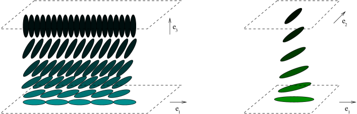
Figure 1. Sketch of the splay-bend director field (left) and of the twisted director field (right).

2.2. Kinematic compatibility

Here, we want to discuss the kinematic compatibility of some given field of (physical) spontaneous strains. Let $\mathcal{O}$ be the (physical) reference configuration of a given system and suppose that it is a simply connected open subset of $\mathbb{R}^{3}$. We say that a smooth map $G:\mathcal{O}\longrightarrow\mathbb{R}^{3{\times}3}$, representing a distribution of spontaneous strains and such that $G(z)\in{\rm Psym}(3)$ for every $z\in\mathcal{O}$, is kinematically compatible if there exists a smooth function $v:\mathcal{O}\longrightarrow\mathbb{R}^{3}$, representing a deformation and such that $\det\nabla v(z)>0$ for every $z\in\mathcal{O}$, satisfying

$$\nabla v^{T}\nabla v=G\qquad\mbox{in}\quad\mathcal{O}.$$ (2.8)

Following [11], we reformulate this concept in the framework of Riemannian geometry. In order to do this, let us denote by $g_{\mathbb{R}^{3}}$ the Euclidean metric of $\mathbb{R}^{3}$ and recall that for a given immersion $\varphi:\mathcal{O}\longrightarrow(\mathbb{R}^{3},g_{\mathbb{R}^{3}})$ the pull-back metric of $g^{\mathbb{R}^{3}}_{|\varphi(\mathcal{O})}$ via $\varphi$ is the metric $h$ defined in $\mathcal{O}$ by the identity

$$h_{|p}(X,Y)\,=\,g^{\mathbb{R}^{3}}_{|\varphi(p)}\left(\,{\rm d}\varphi_{|p}[X],{\rm d}\varphi_{|p}[Y]\,\right),\qquad\qquad\mbox{for every }\quad X,Y\in{\rm T}_{p}\mathcal{O}=\mathbb{R}^{3{\times}3}.$$

The pull-back metric of $g$ via $\varphi$ is usually denoted by $\varphi^{*}\,g_{|\varphi(\mathcal{O})}$. If $(z^{i})_{i=1,2,3}$ and $(x^{\alpha})_{\alpha=1,2,3}$ are systems of coordinates for $\mathcal{O}$ and $\varphi(\mathcal{O})$, respectively, the above identity specialized to $X=\partial/\partial z^{i}_{|p}$ and $Y=\partial/\partial z^{j}_{|p}$ gives

$${h_{ij}}_{|p}\,=\,{g^{\mathbb{R}^{3}}_{\alpha\beta}}_{|\varphi(p)}{\frac{\partial\,\varphi^{\alpha}}{\partial z^{i}}}_{|p}\frac{\partial\,\varphi^{\beta}}{\partial z^{j}}_{|p},$$

where $\varphi^{\alpha}:=x^{\alpha}\circ\varphi$. If, in addition, we assume $(x^{\alpha})_{\alpha=1,2,3}$ to be the standard Euclidean coordinates, then the coefficient ${g^{\mathbb{R}^{3}}_{\alpha\beta}}_{|\varphi(p)}$ is just $\delta_{\alpha\beta}$. Note that here and in what follows the Einstein summation convention for the sum over repeated indices is adopted. We identify the given spontaneous strain distribution $G$ with a metric defined in $\mathcal{O}$, so that asking if there is an orientation-preserving deformation $v:\mathcal{O}\longrightarrow\mathbb{R}^{3}$ such that (2.8) holds true corresponds to seeking for a local diffeomorphism $v:\mathcal{O}\longrightarrow\mathbb{R}^{3}$ such that the pull-back metric of $g_{\mathbb{R}^{3}}$ via $v$ coincides with the metric $G$. In formulas,

$${G_{ij}}_{|p}\,=\,\delta_{\alpha\beta}{\frac{\partial\,v^{\alpha}}{\partial z^{i}}}_{|p}\frac{\partial\,v^{\beta}}{\partial z^{j}}_{|p},$$

where we have fixed standard Euclidean coordinates in the target manifold $v(\mathcal{O})$. Note that since $v$ is a local differmorphism, the equivalence

$$v^{*}g^{\mathbb{R}^{3}}_{|v(\mathcal{O})}=G\qquad\mbox{in}\qquad\mathcal{O}$$ (2.9)

establishes a local isometry (through $v$) between the manifolds $\big{(}\mathcal{O},G\big{)}$ and $\Big{(}v(\mathcal{O}),g^{\mathbb{R}^{3}}_{|v(\mathcal{O})}\Big{)}$. Now, we have from Theorem 1.5-1 and Theorem 1.6-1 in [11] that, since $\mathcal{O}$ is simply connected, a necessary and sufficient condition for (2.9) to hold is that

$${\rm Riem}_{G}\equiv 0\qquad\mbox{in}\qquad\mathcal{O},$$ (2.10)

where ${\rm Riem}_{G}$ is the fourth-order Riemann curvature tensor associated with the metric $G$. We recall that, in the given local chart $(z^{i})_{i=1,2,3}$ of $\mathcal{O}$, the $(3,1)$–coefficients ${\rm R}_{ijk}^{l}$’s of ${\rm Riem}_{G}={\rm R}_{ijk}^{l}\big{(}{\rm d}z^{i}\otimes{\rm d}z^{j}\otimes{\rm d}z^{k}\otimes\partial/\partial z^{l}\big{)}$ are given by

$${\rm R}_{ijk}^{l}\,:=\,\frac{\partial}{\partial z^{j}}\Gamma_{ik}^{l}-\frac{\partial}{\partial z^{k}}\Gamma_{ij}^{l}+\Gamma_{js}^{l}\Gamma_{ik}^{s}-\Gamma_{ks}^{l}\Gamma_{ij}^{s},$$

where the Christoffel’s symbols $\Gamma_{ij}^{k}$’s are defined as

$$\Gamma_{ij}^{k}\,:=\,G^{kl}\,\Gamma_{ijl},\qquad\qquad\Gamma_{ijl}\,:=\,\frac{1}{2}\Big{(}\partial_{i}G_{jl}+\partial_{j}G_{il}-\partial_{l}G_{ij}\Big{)},$$ (2.11)

and the symbols $G^{ij}$’s stand for the components of the inverse $G^{-1}$ of $G$. To simplify the computations it is sometimes useful to introduce the $(4,0)$–coefficients ${\rm R}_{lijk}$’s of ${\rm Riem}_{L}$, defined as

$${\rm R}_{lijk}\,:=\,G_{ls}\,{\rm R}_{ijk}^{s}\,=\,\partial_{j}\Gamma_{ikl}-\partial_{k}\Gamma_{ijl}+\Gamma_{ij}^{p}\Gamma_{klp}+\Gamma_{ik}^{p}\Gamma_{jlp}.$$

It is clear that ${\rm Riem}_{G}\equiv 0$ if and only if ${\rm R}_{lijk}\equiv 0$ for every $l,i,j,k\in\{1,2,3\}$. Finally, let us recall that, since we are in dimension $3$, condition (2.10) is equivalent to ${\rm Ric}_{G}\equiv 0$ in $\mathcal{O}$, where ${\rm Ric}_{G}$ denotes the second-order Ricci curvature tensor associated with $G$, which is defined as ${\rm Ric}_{G}={\rm R}_{ij}\,{\rm d}z^{i}\otimes{\rm d}z^{j}$, with

$${\rm R}_{ij}\,:=\,\partial_{l}\Gamma_{ij}^{l}-\partial j\Gamma_{il}^{l}+\Gamma_{lk}^{l}\Gamma_{ij}^{k}-\Gamma_{jk}^{l}\Gamma_{il}^{k}.$$

From now on in this section, we restrict our attention to the case where $\mathcal{O}=\Omega_{h}$ (see (2.1)) and the spontaneous strain distribution $G$ is a function of the thickness variable $z_{3}\in(-h/2,h/2)$. Note that a material point of $\Omega_{h}$, normally referred to as a point of components $(z_{1},z_{2},z_{3})$ throughout the paper, is a point of the manifold $\Omega_{h}$ with coordinates $(z^{1},z^{2},z^{3})$ from the point of view of Riemannian geometry. In the following subsections, we discuss the kinematic compatibility of $z_{3}\mapsto G(z_{3})$ in three cases: the case where $G(z_{3})$ depends quadratically on $z_{3}$ and two cases (splay-bend and twisted nematic elastomer sheets) where the dependence of $G(z_{3})$ on $z_{3}$ is more complicated and gives rise to incompatible strains. Throughout this section we use the variable $t$ in place of $z_{3}$ and we use the index/apex “$t$” in place of “$3$”.

2.2.1. The splay-bend case

In this case, setting

$$f_{h}(t):=\frac{\pi}{4}+\frac{\pi}{2h}t,\qquad\qquad t\in(-h/2,h/2),$$ (2.12)

and looking at (2.3) and (2.7), we have that, up to a multiplicative constant, the spontaneous strain distribution is given by

$$G=G(t) ={\rm I}+(a_{h}-1)n^{h}_{SB}\otimes n^{h}_{SB}=\left(\begin{array}[]{ccc}1+(a_{h}-1)\cos^{2}f_{h}&0&\left(\frac{a_{h}-1}{2}\right)\sin(2f_{h})\\ 0&1&0\\ \left(\frac{a_{h}-1}{2}\right)\sin(2f_{h})&0&1+(a_{h}-1)\cos^{2}f_{h}\end{array}\right),$$

$$G^{-1}(t) ={\rm I}+\left(\frac{1}{a_{h}}-1\right)n^{h}_{SB}\otimes n^{h}_{SB}=\left(\begin{array}[]{ccc}1+\left(\frac{1}{a_{h}}-1\right)\cos^{2}f_{h}&0&\left(\frac{1-a_{h}}{2a_{h}}\right)\sin(2f_{h})\\ 0&1&0\\ \left(\frac{1-a_{h}}{2a_{h}}\right)\sin(2f_{h})&0&1+\left(\frac{1}{a_{h}}-1\right)\cos^{2}f_{h}\end{array}\right).$$

It turns out that the coefficient ${\rm R}_{1t}$ of ${\rm Ric}_{G}$ has the quite simple expression

$$R_{1t}\,:=\,\partial_{l}\Gamma_{1t}^{l}-\partial_{t}\Gamma_{1l}^{l}+\Gamma_{lk}^{l}\Gamma_{1t}^{k}+\Gamma_{tk}^{l}\Gamma_{1l}^{k}\,=\,-\partial_{t}(\Gamma_{11}^{1}+\Gamma_{12}^{2})+\Gamma_{lk}^{l}\Gamma_{1t}^{k}+\Gamma_{tk}^{l}\Gamma_{1l}^{k}\,=\,-\partial_{t}\Gamma_{11}^{1}+\Gamma_{1t}^{1}\Gamma_{1t}^{t}+\Gamma_{tt}^{1}\Gamma_{11}^{t},$$ (2.13)

where we have first used the fact that the Christoffel symbols depend only on $t$ and secondly the property

$$\Gamma_{ij}^{k}=0\qquad\mbox{whenever}\qquad 2\in\{i,j,k\}.$$

This can be easily checked using the definition of $\Gamma_{ij}^{k}$ in (2.11). The same definition and simple computations also give

$$\Gamma_{11}^{1} \,=\,-\Gamma_{1t}^{t}\,=\,-\frac{(a-1)^{2}}{a}\left(\frac{\pi}{2h}\right)\sin^{2}f_{h}\cos^{2}f_{h},$$

$$\Gamma_{1t}^{1} \,=\,-(a-1)\left(\frac{\pi}{2h}\right)\sin f_{h}\cos f_{h}\left[1+\left(\frac{1}{a}-1\right)\cos^{2}f_{h}\right],$$

$$\Gamma_{tt}^{1} \,=\,(a-1)\left(\frac{\pi}{2h}\right)(\cos^{2}f_{h}-\sin^{2}f_{h})\left[1+\left(\!\frac{1}{a}-1\!\right)\sin^{2}f_{h}\right]-\frac{(a-1)^{2}}{a}\left(\frac{\pi}{2h}\right)\sin^{2}f_{h}\cos^{2}f_{h},$$

$$\Gamma_{11}^{t} \,=\,(a-1)\left(\frac{\pi}{2h}\right)\sin f_{h}\cos f_{h}\left[1+\left(\!\frac{1}{a}-1\!\right)\sin^{2}f_{h}\right]\!.$$

Plugging these expressions into (2.13) yields

$${\rm R}_{1t}=-\frac{(a-1)^{2}}{a}\left(\frac{\pi}{2h}\right)\sin f_{h}\cos f_{h}(\cos^{2}f_{h}-\sin^{2}f_{h})=-\frac{(a-1)^{2}}{a}\left(\frac{\pi}{8h}\right)\sin\left(\pi+\frac{2\pi}{h}t\right).$$

Thus, we can conclude that ${\rm R}_{1t}$ is not identically zero in $\Omega_{h}$. In turn, ${\rm Ric}_{G}$ is not identically zero, so that the splay-bend spontaneous strain distribution is not kinematically compatible.

2.2.2. The twisted case

In this case, following the same notation as in (2.12), we have

$$G=G(t) ={\rm I}+(a_{h}-1)n^{h}_{T}\otimes n^{h}_{T}=\left(\begin{array}[]{ccc}1+(a_{h}-1)\cos^{2}f_{h}&\left(\frac{a_{h}-1}{2}\right)\sin(2f_{h})&0\\ \left(\frac{a_{h}-1}{2}\right)\sin(2f_{h})&1+(a_{h}-1)\cos^{2}f_{h}&0\\ 0&0&1\\ \end{array}\right),$$

$$G^{-1}(t) ={\rm I}+\left(\frac{1}{a_{h}}-1\right)n^{h}_{T}\otimes n^{h}_{T}=\left(\begin{array}[]{ccc}1+\left(\frac{1}{a_{h}}-1\right)\cos^{2}f_{h}&\left(\frac{1-a_{h}}{2a_{h}}\right)\sin(2f_{h})&0\\ \left(\frac{1-a_{h}}{2a_{h}}\right)\sin(2f_{h})&1+\left(\frac{1}{a_{h}}-1\right)\cos^{2}f_{h}&0\\ 0&0&1\end{array}\right).$$

For the twisted geometry, the coefficient ${\rm R}_{tt}$ of ${\rm Ric}_{G}$ has a simple expression. Indeed, we have

$${\rm R}_{tt}\,:=\,\partial_{l}\Gamma_{tt}^{l}-\partial_{t}\Gamma_{tl}^{l}+\Gamma_{lk}^{l}\Gamma_{tt}^{k}+\Gamma_{tk}^{l}\Gamma_{tl}^{k}\,=\,-\partial_{t}(\Gamma_{1t}^{1}+\Gamma_{2t}^{2})-\big{(}\Gamma_{tk}^{1}\Gamma_{1t}^{k}+\Gamma_{tk}^{2}\Gamma_{2t}^{k}\big{)}\,=\,-\Big{[}(\Gamma_{1t}^{1})^{2}+2\,\Gamma_{1t}^{2}\Gamma_{2t}^{1}+(\Gamma_{2t}^{2})^{2}\Big{]},$$ (2.14)

since

$$\Gamma_{tt}^{k}=0\quad\mbox{for every}\quad k=1,2,t,\qquad\mbox{and}\qquad\Gamma_{1t}^{1}\,=\,-\Gamma_{2t}^{2}\,=\,-\left(\frac{a^{2}-1}{2a}\right)\left(\frac{\pi}{2h}\right)\sin f_{h}\cos f_{h}.$$ (2.15)

This can be easily checked from the definition of the Christoffel symbols in (2.11). Similar computations yield

$$\Gamma_{1t}^{2}\,=\,\left(\frac{a-1}{2}\right)\left(\frac{\pi}{2h}\right)\left(\cos^{2}f_{h}-\frac{\sin^{2}f_{h}}{a}\right),\qquad\Gamma_{2t}^{1}\,=\,\left(\frac{a-1}{2}\right)\left(\frac{\pi}{2h}\right)\left(\frac{\cos^{2}f_{h}}{a}-\sin^{2}f_{h}\right).$$

Using these formulas together with (2.14) and the second equation in (2.15) gives

$${\rm R}_{tt}\,=\,-\frac{(a-1)^{2}}{2a}\left(\frac{\pi}{2h}\right)^{2}.$$

This fact implies, in particular, that ${\rm Ric}_{G}$ is not identically zero and in turn that the twisted spontaneous strain distribution is not kinematically compatible.

2.2.3. The quadratic case

In this subsection, we consider the case where

$$G\,=\,G(t)\,=\,{\rm I}+t\,A+t^{2}\,B,\qquad\qquad t\in(-h/2,h/2),$$ (2.16)

for some diagonal matrices $A={\rm diag}(A_{11},A_{22},A_{tt})$ and $B={\rm diag}(B_{11},B_{22},B_{tt})$. Note that $G(t)=:{\rm diag}(G_{11}(t),G_{22}(t),G_{tt}(t))$ is positive definite for every $t$ sufficiently small. Elementary computations yield

$${\rm R}_{11} =-\frac{1}{4}\left(\frac{G_{11}}{G_{tt}}\right)\left\{2\frac{\rm d}{{\rm d}t}\left(\frac{\dot{G}_{11}}{G_{11}}\right)+\left(\frac{\dot{G}_{11}}{G_{11}}\right)\left[\frac{\dot{G}_{11}}{G_{11}}+\frac{\dot{G}_{22}}{G_{22}}-\frac{\dot{G}_{tt}}{G_{tt}}\right]\right\},$$

$${\rm R}_{22} =-\frac{1}{4}\left(\frac{G_{22}}{G_{tt}}\right)\left\{2\frac{\rm d}{{\rm d}t}\left(\frac{\dot{G}_{22}}{G_{22}}\right)+\left(\frac{\dot{G}_{22}}{G_{22}}\right)\left[\frac{\dot{G}_{11}}{G_{11}}+\frac{\dot{G}_{22}}{G_{22}}-\frac{\dot{G}_{tt}}{G_{tt}}\right]\right\},$$

$${\rm R}_{tt} =-\frac{1}{4}\left\{2\frac{\rm d}{{\rm d}t}\left(\frac{\dot{G}_{11}}{G_{11}}+\frac{\dot{G}_{22}}{G_{22}}\right)-\left(\frac{\dot{G}_{tt}}{G_{tt}}\right)\left(\frac{\dot{G}_{11}}{G_{11}}+\frac{\dot{G}_{22}}{G_{22}}\right)+\left(\frac{\dot{G}_{11}}{G_{11}}\right)^{2}+\left(\frac{\dot{G}_{22}}{G_{22}}\right)^{2}\right\},$$

$${\rm R}_{ij} =0,\qquad\mbox{for every }i\neq j,$$

where $\dot{G}_{ii}$ is the derivative of $G_{ii}$ with respect to $t$. Now, set

$$\xi:=\log G_{11},\qquad\quad\eta:=\log G_{22},\qquad\quad\tau:=\log G_{tt},$$

so that $\dot{G}_{11}/G_{11}=\dot{\xi}$, $\dot{G}_{22}/G_{22}=\dot{\eta}$, $\dot{G}_{tt}/G_{tt}=\dot{\tau}$, and in turn

$${\rm R}_{11} \,=\,-\frac{1}{4}\left(\frac{{\rm e}^{\xi}}{{\rm e}^{\tau}}\right)\left[2\,\ddot{\xi}+\dot{\xi}\left(\dot{\xi}+\dot{\eta}-\dot{\tau}\right)\right],\qquad\qquad{\rm R}_{22}\,=\,-\frac{1}{4}\left(\frac{{\rm e}^{\eta}}{{\rm e}^{\tau}}\right)\left[2\,\ddot{\eta}+\dot{\eta}\left(\dot{\xi}+\dot{\eta}-\dot{\tau}\right)\right],$$

$${\rm R}_{tt} \,=\,-\frac{1}{4}\left[2\,(\ddot{\xi}+\ddot{\eta})-\dot{\tau}\,(\dot{\xi}+\dot{\eta})+(\dot{\xi})^{2}+(\dot{\eta})^{2}\right].$$

The condition ${\rm Ric}_{G}\equiv 0$, which guarantees the kinematic compatibility of $t\mapsto G(t)$ as discussed above, is then equivalent to the following system of ODEs:

$$\begin{cases}&2\,\ddot{\xi}+\dot{\xi}\left(\dot{\xi}+\dot{\eta}-\dot{\tau}\right)=0,\\ &2\,\ddot{\eta}+\dot{\eta}\left(\dot{\xi}+\dot{\eta}-\dot{\tau}\right)=0,\\ &2\,(\ddot{\xi}+\ddot{\eta})-\dot{\tau}\,(\dot{\xi}+\dot{\eta})+(\dot{\xi})^{2}+(\dot{\eta})^{2}=0.\end{cases}$$

Solving this system translates into compatibility conditions on $A$ and $B$ in (2.16). It then turns out that a spontaneous strain distribution $t\mapsto G(t)$ of the form (2.16) is kinematically compatible if and only if one of the following four conditions is satisfied:

$$(i)\quad A_{11}=A_{22}=A_{tt}=0\quad\mbox{and}\quad B_{11}=B_{22}=B_{tt}=0,$$

$$(ii)\quad A_{22}=A_{tt}=0,\quad B_{22}=B_{tt}=0,\quad\mbox{and}\quad B_{11}=A_{11}^{2}/4\neq 0,$$

$$(iii)\quad A_{11}=A_{tt}=0,\quad B_{11}=B_{tt}=0,\quad\mbox{and}\quad B_{22}=A_{22}^{2}/4\neq 0,$$

$$(iv)\quad A_{11}=A_{22}=0,\quad B_{11}=B_{22}=0,\quad\mbox{and}\quad A_{tt}^{2}+B_{tt}^{2}\neq 0.$$

Note that the first condition corresponds to the trivial case $G={\rm I}$ and the second one tells us in particular that a strain of the form

$$G(t):=\left(\begin{array}[]{ccc}1-2\,k\,t+k^{2}\,t^{2}&0&0\\ 0&1&0\\ 0&0&1\end{array}\right),\qquad\qquad t\in(-h/2,h/2),$$ (2.17)

for some constant $k\in\mathbb{R}\setminus\{0\}$, is kinematically compatible. A prototypical deformation $v$ giving rise to such $G$ can be provided in the following way. Let $I$ be an open interval of $\mathbb{R}$, let $\gamma:I\longrightarrow\mathbb{R}^{3}$ be a smooth curve, and define

$$T(s):=\gamma^{\prime}(s),\qquad\qquad N(s):=\frac{T^{\prime}(s)}{|T^{\prime}(s)|},\qquad\qquad B(s):=T(s)\wedge N(s),$$

for every $s\in I$, where the apex stands for differentiation with respect to $s$. Suppose that the curve is parameterized by arc length, so that $|T|=1$ and the curvature $k$ is defied as $k:=|T^{\prime}|$. Then the Frenet–Serret formulas read

$$\begin{cases}T^{\prime}&=\ k\,N,\\ N^{\prime}&=\ -k\,T+\tau\,B,\\ B^{\prime}&=\ -\tau\,N.\end{cases}$$

Note that multiplying the first equation by $N$ gives $k=T^{\prime}\cdot N=-N^{\prime}\cdot T$. Let us restrict to the case of $B$ being constantly equal to $\mathsf{e}_{2}$, where $\{\mathsf{e}_{1},\mathsf{e}_{2},\mathsf{e}_{2}\}$ is the canonical basis of $\mathbb{R}^{3}$. This means that $\gamma$ is a planar curve and the above formulas imply in particular that $\tau=-B^{\prime}\cdot N=0$ and $|N^{\prime}|^{2}=k^{2}$. Now, let us define $v:\Omega_{h}\longrightarrow\mathbb{R}^{3}$ as

$$v(s,z_{2},t)\,:=\,\gamma(s)+t\,N(s)+z_{2}\,\mathsf{e}_{2},$$

where we have supposed $\omega_{h}=\omega\times(-h/2,h/2)$ with $\omega=I\times J$, for some open intervals $I$, $J\subset\mathbb{R}$. Then $\nabla v=(T+t\,N^{\prime}\,|\,\mathsf{e}_{2}\,|\,N)$ and therefore

$$\nabla v^{T}\nabla v=\left(\begin{array}[]{ccc}|T|^{2}+2\,t\,T{\cdot}N^{\prime}+t^{2}|N^{\prime}|^{2}&\mathsf{e}_{2}{\cdot}(T+t\,N^{\prime})&N{\cdot}(T+t\,N^{\prime})\\ \mathsf{e}_{2}{\cdot}(T+t\,N^{\prime})&|\mathsf{e}_{2}|^{2}&\mathsf{e}_{2}\cdot N\\ N{\cdot}(T+t\,N^{\prime})&\mathsf{e}_{2}\cdot N&|N|^{2}\end{array}\right)=\left(\begin{array}[]{ccc}1-2\,k\,t+k^{2}\,t^{2}&0&0\\ 0&1&0\\ 0&0&1\end{array}\right).$$

Supposing the curvature $k$ to be constant, we have thus derived a strain $G$ of the form (2.17).

Finally, note that the analysis performed in this session shows that in the linear case where $G(t)$ is of the form

$$G\,=\,G(t)\,=\,{\rm I}+t\,A,\qquad\qquad t\in(-h/2,h/2),$$

for some diagonal matrix $A\neq 0$, the kinematic compatibility of the spontaneous strain distribution is never fulfilled.

3. Derivation of the plate model

In this section, we first rewrite the three-dimensional model previously introduced in a rescaled reference configuration. Then, in Subsection 3.2, we recall two rigorous dimension reduction results of compactness and $\Gamma$-convergence. This mathematical technique is subsequently employed in Subsection 3.3, where our main results, Theorems 3.5 and 3.7, are stated and proved.

3.1. The rescaled three-dimensional model

As it is standard for dimension reduction techniques, let us now operate a change of variables in order to rewrite the energies in a fixed, $h$-independent rescaled reference configuration.

Notation 3.1.

We denote by $x=(x_{1},x_{2},x_{3})=(x^{\prime},x_{3})$ an arbitrary point in the rescaled reference configuration $\Omega:=\omega\times(-1/2,1/2)$.

For every $h>0$ small, we define the rescaled energy density $W^{h}:(-1/2,1/2)\times\mathbb{R}^{3\times 3}\longrightarrow[0,+\infty]$ and the rescaled applied loads $f_{h}:\Omega\longrightarrow\mathbb{R}^{3}$ as

$$W^{h}(x_{3},F)\,:=\,w^{h}(hx_{3},F),\qquad\qquad\quad f_{h}(x)\,:=\,\hat{f}_{h}(x^{\prime},hx_{3}).$$ (3.1)

Note that $W^{h}$ fulfills

$$W^{h}(x_{3},F)=0\qquad\quad\mbox{iff}\qquad\quad F\in{\rm SO}(3)\sqrt{\overline{C}_{h}(z_{3})},\qquad\qquad\overline{C}_{h}(x_{3}):=\bar{c}_{h}(hx_{3}).$$

Setting

$$\nabla_{h}y:=\left(\begin{array}[]{ccccc}\!\!\partial_{x_{1}}y\!\!&\!\!\bigg{|}\!\!&\!\!\partial_{x_{2}}y\!\!&\!\!\bigg{|}\!\!&\!\!\displaystyle\frac{\partial_{x_{3}}y}{h}\!\!\end{array}\right)=:\left(\begin{array}[]{ccccc}\!\!\nabla^{\prime}y\!\!&\!\!\bigg{|}\!\!&\!\!\displaystyle\frac{\partial_{x_{3}}y}{h}\!\!\end{array}\right),\qquad\qquad\mbox{for every}\quad y:\Omega\longrightarrow\mathbb{R}^{3},$$ (3.2)

the correspondence between the original quantities and the rescaled ones is through the formulas

$$\hat{\mathscr{E}}^{h}(v)\,=\,h\,\mathscr{E}^{h}(y),\qquad\quad\hat{\mathscr{F}}^{h}(v)\,=\,h\,\mathscr{F}^{h}(y),\qquad\qquad v(z):=y(z^{\prime},z_{3}/h)\quad\mbox{a.e.}\ z\ \mbox{in}\ \Omega_{h}.$$ (3.3)

Here, the rescaled stored elastic energy functional $\mathscr{E}^{h}$ and the rescaled total energy functional $\mathscr{F}^{h}$ are defined, on a deformation $y:\Omega\to\mathbb{R}^{3}$, as

$$\mathscr{E}^{h}(y):=\int\limits_{\Omega}W^{h}(x_{3},\nabla_{h}y(x))\,{\rm d}x,\qquad\qquad\mathscr{F}^{h}(y)\,:=\,\mathscr{E}^{h}(y)-\int\limits_{\Omega}f_{h}\cdot y\,{\rm d}x.$$ (3.4)

Following the notation already introduced in Section 2.1, we use the indexes $SB$ and $T$ to denote the quantities related to the splay-bend case and twisted case, respectively. Hence, we write $\overline{C}_{h,SB}$, $W^{h}_{SB}$, $\mathscr{E}^{h}_{SB}$, and $\mathscr{F}^{h}_{SB}$ for the splay-bend model, and $\overline{C}_{h,T}$, $W^{h}_{T}$, $\mathscr{E}^{h}_{T}$, and $\mathscr{F}^{h}_{T}$ for the twisted model.

We now focus attention on the (rescaled) spontaneous strains $\overline{C}_{h}(x_{3})$. Looking at (2.7), we first note that for both models $n^{h}(hx_{3})$ is independent of $h$, namely

$$N_{SB}(x_{3}):=n^{h}_{SB}(hx_{3})=\left(\begin{array}[]{c}\cos\big{(}\frac{\pi}{4}+\frac{\pi}{2}x_{3}\big{)}\\ 0\\ \sin\big{(}\frac{\pi}{4}+\frac{\pi}{2}x_{3}\big{)}\end{array}\right),\qquad\quad N_{T}(x_{3}):=n^{h}_{T}(hx_{3})=\left(\begin{array}[]{c}\cos\big{(}\frac{\pi}{4}+\frac{\pi}{2}x_{3}\big{)}\\ \sin\big{(}\frac{\pi}{4}+\frac{\pi}{2}x_{3}\big{)}\\ 0\end{array}\right),$$ (3.5)

for every $x_{3}\in(-1/2,1/2)$. Hence, referring to the (above) definition of $\overline{C}_{h}$ and to expression (2.3), we have for the splay-bend case as well as for the twisted case

$$\overline{C}_{h}(x_{3}) =a_{h}^{2/3}N(x_{3})\otimes N(x_{3})+a_{h}^{-1/3}\big{(}{\rm I}-N(x_{3})\otimes N(x_{3})\big{)}$$

$$=\big{(}a_{h}^{2/3}-a_{h}^{-1/3}\big{)}\left(\frac{{\rm I}}{a_{h}-1}+N(x_{3})\otimes N(x_{3})\right)$$

$$={\rm I}+\frac{\alpha_{0}h}{h_{0}}\left(N(x_{3})\otimes N(x_{3})-\frac{{\rm I}}{3}\right)+R^{h}(x_{3}),$$ (3.6)

where $\|R^{h}\|_{\infty}=o(h)$ and $\|\cdot\|_{\infty}$ is the norm in the space ${\rm L}^{\infty}\big{(}(-1/2,1/2),\mathbb{R}^{3\times 3}\big{)}$. Note that in the third equality we have plugged in expression (2.4) for $a_{h}$ and used the expansion

$$a_{h}^{2/3}-a_{h}^{-1/3}=\frac{\alpha_{0}h}{h_{0}}-\frac{1}{3}\left(\frac{\alpha_{0}h}{h_{0}}\right)^{2}+o(h^{2}).$$

3.2. A rigorous mathematical result for the limiting theory

For the convenience of the reader, we collect in this section, in a slightly simplified version, two results proved in [32] (Theorems 3.3 and 3.4 below), which we are going to use later on. In this paper, an arbitrary family of energy densities $W^{h}:(-1/2,1/2)\times\mathbb{R}^{3\times 3}\longrightarrow[0,+\infty]$ is considered, with the property that

$$W^{h}(x_{3},F)\,=\,W_{0}\big{(}F({\rm I}+hB^{h}(x_{3}))\big{)},$$ (3.7)

where the function $W_{0}:\mathbb{R}^{3\times 3}\longrightarrow[0,+\infty]$ satisfies Assumption 3.2 below, and

$$B^{h}\longrightarrow B\qquad\qquad\mbox{in}\qquad{\rm L}^{\infty}((-1/2,1/2),\mathbb{R}^{3\times 3}),\qquad\mbox{as}\quad h\downarrow 0.$$

For each small $h$, let us introduce the functional $\mathscr{E}^{h}:{\rm W}^{1,2}(\Omega,\mathbb{R}^{3})\to[0,+\infty]$, defined as

$$\mathscr{E}^{h}(y)\;:=\,\int\limits_{\Omega}W^{h}(x_{3},\nabla_{h}y){\rm d}x,$$

with $\nabla_{h}$ given by (3.2). Recall that here and throughout the paper $\Omega=\omega\times(-1/2,1/2)$ and $\omega\subset\mathbb{R}^{2}$ is a bounded Lipschitz domain with sufficiently regular boundary. More precisely, for the following theorems to hold, it is required that there exists a closed subset $\Sigma\subset\partial\omega$ with $\mathscr{H}^{1}(\Sigma)=0$ such that the outer unit normal exists and is continuous on $\partial\omega\setminus\Sigma$.

Assumption 3.2.

The function $W_{0}:\mathbb{R}^{3\times 3}\longrightarrow[0,+\infty]$ fulfills the following conditions:

• it is ${\rm C}^{2}$ in a neighborhood of ${\rm SO}(3)$, and it is minimised at ${\rm I}$;

• it is frame-indifferent, i.e. $W_{0}(F)=W_{0}(RF)$ for every $R\in{\rm SO}(3)$.

• there exists a constant $C>0$ such that for every $F\in\mathbb{R}^{3{\times}3}$,

  $$W_{0}(F)\,\geq\,C\,{\rm dist}^{2}\big{(}F,{\rm SO}(3)\big{)}.$$

The following result states that a sequence $\{y_{h}\}$ which bounds the energy $\mathscr{E}^{h}$ by a factor $h^{2}$ converges (up to subsequences) to a limit that is constrained to the class of (${\rm W}^{2,2}$-) isometric immersions of $\omega$ into the three-dimensional Euclidean space, namely

$$\mathcal{A}_{iso}\,:=\,\Big{\{}y\in{\rm W}^{2,2}(\omega,\mathbb{R}^{3}):(\nabla^{\prime}y)^{T}\nabla^{\prime}y={\rm I}_{2}\ \mbox{\ }{a.e.\ in}\quad\omega\Big{\}}.$$ (3.8)

Theorem 3.3 (Compactness).

If $\{y^{h}\}\subset{\rm W}^{1,2}(\Omega,\mathbb{R}^{3})$ is a sequence such that

$$\int\limits_{\Omega}W^{h}(x_{3},\nabla_{h}y_{h}){\rm d}x\leq Ch^{2}$$ (3.9)

for every $h>0$ small, then there exists a (not relabelled) subsequence such that

$$\nabla_{h}y^{h}\longrightarrow\left(\begin{array}[]{ccccc}\!\!\nabla^{\prime}y\!\!&\!\!\big{|}\!\!&\!\!\nu\!\!\end{array}\right),\qquad\mbox{as}\quad h\downarrow 0,\quad\text{strongly in}\quad{\rm L}^{2}(\Omega,\mathbb{R}^{3{\times}3}).$$

Moreover, the function $x\mapsto\left(\begin{array}[]{ccc}\!\!\nabla^{\prime}y\!\!&\!\!\big{|}\!\!&\!\!\nu\!\!\end{array}\right)$ belongs to ${\rm W}^{1,2}(\Omega,\mathbb{R}^{3\times 3})$, is independent of $x_{3}$, and
$\left(\begin{array}[]{ccc}\!\!\nabla^{\prime}y\!\!&\!\!\big{|}\!\!&\!\!\nu\!\!\end{array}\right)(x^{\prime})\in{\rm SO}(3)$ for a.e. $x^{\prime}\in\omega$.

Before proceeding, let us introduce some more notation and denote by $Q_{3}(M)$, $M\in\mathbb{R}^{3\times 3}$, the quadratic form ${\rm D}^{2}W_{0}({\rm I})[M,M]$, where ${\rm D}^{2}W_{0}({\rm I})$ stands for the second differential of $W_{0}$ evaluated at ${\rm I}$. Moreover, define, for every $G\in\mathbb{R}^{2\times 2}$,

$$Q_{2}(G)\,:=\,\min_{\stackrel{{\scriptstyle b\in\mathbb{R}^{2}}}{{a\in\mathbb{R}}}}Q_{3}\left(\left[\begin{tabular}[]{c|c}$G$&$b$\\ \hline\cr$0$&$a$\end{tabular}\right]\right),$$ (3.10)

and in turn

$$\overline{Q}_{2}(G)\,:=\,\min_{D\in\mathbb{R}^{2\times 2}}\int\limits_{-1/2}^{1/2}Q_{2}\big{(}D+t\,G+\check{B}(t)\big{)}{\rm d}t,$$ (3.11)

where $\check{B}$ is obtained from $B$ by omitting the last row and the last column.

Theorem 3.4 ($\Gamma$-convergence).

The functionals $\mathscr{E}^{h}/h^{2}$ $\Gamma$-converge as $h\downarrow 0$, with respect to the strong and the weak topology of ${\rm W}^{1,2}(\Omega,\mathbb{R}^{3})$, to

$$\mathscr{E}^{lim}(y)\,:=\,\left\{\begin{array}[]{ll}\displaystyle\frac{1}{2}\int\limits_{\omega}\overline{Q}_{2}(A_{y}(x^{\prime})){\rm d}x^{\prime}&\qquad\mbox{if}\quad y\in\mathcal{A}_{iso},\\ &\\ +\infty&\qquad\mbox{otherwise in}\quad{\rm W}^{1,2}(\Omega,\mathbb{R}^{3}),\end{array}\right.$$

where $A_{y}$ denotes the second fundamental form associated with the surface $y(\omega)$.

Recall that the second fundamental form of $y(\omega)$ at a point $y(x^{\prime})$ can be expressed as $\big{(}\nabla^{\prime}y(x^{\prime})\big{)}^{T}\nabla^{\prime}\nu(x^{\prime})$, where $\nu:=\partial_{x_{1}}y\wedge\partial_{x_{2}}y$.

3.3. Splay-bend and twisted nematic elastomer plates

We want to apply the theory presented in the previous section to our two models. We first focus on the splay-bend case, whose associated rescaled stored energy density, considering expression (2.5) together with(3.1) and (3.1), is given, for every $x_{3}\in(-1/2,1/2)$ and every $F\in\mathbb{R}^{3\times 3}$ with $\det F>0$, by

$$W^{h}_{SB}(x_{3},F)\,=\,\frac{\mu}{2}\Big{[}(F^{T}F)\cdot\overline{C}_{h,SB}^{-1}(x_{3})-3-2\log(\det F)\Big{]}+W_{vol}(\det F).$$

Recall that

$$\overline{C}_{h,SB}(x_{3})={\rm I}+\frac{\alpha_{0}h}{h_{0}}\left(N_{SB}(x_{3})\otimes N_{SB}(x_{3})-\frac{{\rm I}}{3}\right)+R^{h}_{SB}(x_{3}),\qquad\quad\|R^{h}_{SB}\|_{\infty}=o(h)$$ (3.12)

(see (3.5) for the definition of $N_{SB}$). Defining

$$W_{0}(F)\,:=\,\frac{\mu}{2}\Big{[}|F|^{2}-3-2\log(\det F\,)\Big{]}+W_{vol}(\det F\,),$$ (3.13)

for every $F\in\mathbb{R}^{3\times 3}$ with $\det F>0$, and setting

$$\overline{U}_{h,SB}:=\sqrt{\overline{C}_{h,SB}},$$ (3.14)

yields $W^{h}_{SB}(x_{3},F)=W_{0}\big{(}F\overline{U}_{h,SB}^{-1}(x_{3})\big{)}$. Note that

$$\overline{U}_{h,SB}^{-1}={\rm I}+h\left[-\delta_{0}\left(M_{SB}-\frac{{\rm I}}{3}\right)+\frac{r^{h}_{SB}}{h}\right],$$

with $\|r^{h}_{SB}\|_{\infty}=o(h)$, where we have used the notation

$$\delta_{0}:=\frac{\alpha_{0}}{2h_{0}},\qquad\qquad M_{SB}:=N_{SB}\otimes N_{SB}=\left(\begin{array}[]{ccc}\cos^{2}f_{1}&0&\frac{1}{2}\sin(2f_{1})\\ 0&0&0\\ \frac{1}{2}\sin(2f_{1})&0&\sin^{2}f_{1}\end{array}\right).$$ (3.15)

Here, the function $x_{3}\mapsto f_{1}(x_{3})$ is defined as in (2.12), with $h=1$. All in all, we can write

$$W^{h}_{SB}(x_{3},F)=W_{0}\big{(}F({\rm I}+hB^{h}_{SB}(x_{3}))\big{)},\qquad\qquad B^{h}_{SB}:=\left[-\delta_{0}\left(M_{SB}-\frac{{\rm I}}{3}\right)+\frac{r^{h}_{SB}}{h}\right].$$ (3.16)

Since $\|r^{h}_{SB}\|_{\infty}=o(h)$, we have that $B^{h}_{SB}\longrightarrow B_{SB}$ in ${\rm L}^{\infty}\big{(}(-1/2,1/2),\mathbb{R}^{3\times 3}\big{)}$, where $B_{SB}:=-\delta_{0}\left(M_{SB}(x_{3})-\frac{{\rm I}}{3}\right)$. In turn, also in view of Remark 3.6 below, we have shown that the splay-bend model introduced in Section 2.1 perfectly fits the mathematical theory summarized in the previous section. Hence, we have to compute the 2D energy density according to formula (3.11). First of all, we have that $Q_{3}(M)\,=\,2\mu\,|{\rm sym}\,M|^{2}+W_{vol}^{\prime\prime}(1)\,{\rm tr}^{2}M.$ Using this expression, we can compute $Q_{2}$ for every $G\in\mathbb{R}^{2\times 2}$ (see (3.10)):

$$Q_{2}(G) \,=\,\min_{\stackrel{{\scriptstyle b\in\mathbb{R}^{2}}}{{a\in\mathbb{R}}}}\left\{2\mu\left|\left(\begin{tabular}[]{c|c}${\rm sym}\,G$&$b/2$\\ \hline\cr$b^{T}/2$&$a$\end{tabular}\right)\right|^{2}+W_{vol}^{\prime\prime}(1)({\rm tr}\,G+a)^{2}\right\}$$ (3.18)

$$\,=\,2\mu\,|{\rm sym}\,G|^{2}+W_{vol}^{\prime\prime}(1)\,{\rm tr}^{2}G+\min_{a\in\mathbb{R}}\Big{[}\big{(}2\mu+W_{vol}^{\prime\prime}(1)\big{)}a^{2}+2\,W_{vol}^{\prime\prime}(1){\rm tr}\,G\,a\Big{]}\,=\,2\mu\left(|{\rm sym}\,G|^{2}+\gamma\,{\rm tr}^{2}G\right),$$ (3.19)

having introduced the notation

$$\gamma:=\frac{W_{vol}^{\prime\prime}(1)}{2\mu+W_{vol}^{\prime\prime}(1)}.$$ (3.20)

Finally (cfr (3.11)), note that $\check{B}_{SB}$ is given by

$$\check{B}_{SB}=-\delta_{0}\left(\check{M}_{SB}-\frac{{\rm I}_{2}}{3}\right),\qquad\mbox{with}\qquad\check{M}_{SB}(x_{3}):=\big{(}N_{SB}(x_{3})\otimes N_{SB}(x_{3})\big{)}^{\check{}}=\left(\begin{array}[]{cc}\cos^{2}\big{(}\frac{\pi}{4}+\frac{\pi}{2}x_{3}\big{)}&0\\ 0&0\end{array}\right).$$

We are now in the position to compute, for every $G\in\mathbb{R}^{2\times 2}$,

$$\overline{Q}_{2,SB}(G) :=\min_{D\in\mathbb{R}^{2\times 2}}\int\limits_{-1/2}^{1/2}Q_{2}\left(D+t\,G+\check{B}_{SB}(t)\right){\rm d}t$$

$$=2\mu\min_{D\in{\rm Sym}(2)}\int\limits_{-1/2}^{1/2}\!\!\left\{\left|D+t\,{\rm sym}\,G-\delta_{0}\,\check{M}_{SB}(t)+\frac{\delta_{0}}{3}{\rm I}_{2}\right|^{2}\!\!+\gamma\,{\rm tr}^{2}\!\left(D+t\,G-\delta_{0}\,\check{M}_{SB}(t)+\frac{\delta_{0}}{3}{\rm I}_{2}\right)\!\!\right\}{\rm d}t.$$

The integrals

$$\int\limits_{-1/2}^{1/2}|\check{M}_{SB}|^{2}{\rm d}t=\int\limits_{-1/2}^{1/2}\cos^{4}\left(\frac{\pi}{4}+\frac{\pi}{2}t\right){\rm d}t=\frac{3}{8},\qquad\int\limits_{-1/2}^{1/2}t\,{\rm tr}\,\check{M}_{SB}{\rm d}t=\int\limits_{-1/2}^{1/2}t\cos^{2}\left(\frac{\pi}{4}+\frac{\pi}{2}t\right){\rm d}t=-\frac{1}{\pi^{2}}$$

and other elementary computations imply that $\overline{Q}_{2,SB}(G)/(2\mu)$ equals

$$\frac{1}{12}\Big{(}|{\rm sym}\,G|^{2}+\gamma\,{\rm tr}^{2}G\Big{)}+\frac{2\,\delta_{0}}{\pi^{2}}\Big{(}{\rm sym}\,G\cdot{\rm diag}(1,0)+\gamma\,{\rm tr}\,G\Big{)}+\left(\frac{19+11\,\gamma}{72}\right)\delta_{0}^{2}+\min_{D\in{\rm Sym}(2)}q_{SB}(D),$$

where

$$q_{SB}(D):=|D|^{2}+\gamma\,{\rm tr}^{2}D-\delta_{0}\left[{\rm sym}\,D\cdot{\rm diag}(1,0)+\Big{(}\frac{2+\gamma}{3}\Big{)}{\rm tr}\,D\right].$$

It is easy to see that

$$\min_{D\in{\rm Sym}(2)}q_{SB}(D)=q_{SB}\big{(}{\rm diag}(\delta_{0}/6,-\delta_{0}/3)\big{)}=-\Big{(}\frac{5+\gamma}{36}\Big{)}\delta_{0}^{2},$$

and in turn that

$$\overline{Q}_{2,SB}(G)=2\mu\bigg{[}\frac{1}{12}\Big{(}|{\rm sym}\,G|^{2}+\gamma\,{\rm tr}^{2}G\Big{)}+\frac{2\delta_{0}}{\pi^{2}}\Big{(}{\rm sym}\,G\cdot{\rm diag}(1,0)+\gamma\,{\rm tr}\,G\Big{)}+\Big{(}\frac{1+\gamma}{8}\Big{)}\delta_{0}^{2}\bigg{]}.$$

It is again a simple computation showing that there exist constants $\alpha_{SB},\,\beta_{SB}\in\mathbb{R}$ and $\overline{A}_{SB}\in{\rm Sym}(2)$ such that

$$\overline{Q}_{2,SB}(G)\,=\,\alpha_{SB}\,Q_{2}[G-\overline{A}_{SB}]^{2}+\beta_{SB},\qquad\quad\mbox{for every}\quad G\in{\rm Sym}(2),$$ (3.21)

and they are given by

$$\alpha_{SB}\,=\,\frac{1}{12},\quad\qquad\overline{A}_{SB}\,=\,\frac{12\delta_{0}}{\pi^{2}}\,{\rm diag(-1,0)},\quad\qquad\beta_{SB}\,=\,\mu\,(1+\gamma)\delta_{0}^{2}\Big{(}\frac{\pi^{4}-12}{4}\Big{)}.$$ (3.22)

To state our result, let us define the functional $\mathscr{E}^{lim}_{SB}:\mathcal{A}_{iso}\longrightarrow[0,\infty)$, where $\mathcal{A}_{iso}$ is the class defined in (3.8), as

$$\mathscr{E}^{lim}_{SB}(y) :=\frac{1}{2}\int\limits_{\omega}\overline{Q}_{2,SB}(A_{y}(x^{\prime})){\rm d}x^{\prime}$$

$$=\frac{\mu}{12}\int\limits_{\omega}\!\!\left\{\Big{|}{\rm A}_{y}(x^{\prime})\!-\!\frac{12\delta_{0}}{\pi^{2}}\,{\rm diag}\big{(}-1,0\big{)}\Big{|}^{2}\!\!+\gamma\Big{(}{\rm H}_{y}(x^{\prime})\!+\!\frac{12\delta_{0}}{\pi^{2}}\Big{)}^{2}\!\right\}\!{\rm d}x^{\prime}+\mu\,(1+\gamma)\delta_{0}^{2}\Big{(}\frac{\pi^{4}-12}{8}\Big{)}\!|\omega|.$$ (3.23)

Here, the symbol ${\rm H}_{y}$ denotes the mean curvature of $y(\omega)$, hence ${\rm H}_{y}={\rm tr}A_{y}$. Note that for every $y\in\mathcal{A}_{iso}$ we have that $|{\rm A}_{y}|\in{\rm L}^{2}(\omega)$, and in turn $\mathscr{E}^{lim}_{SB}(y)<+\infty$.

Theorems 3.3 and 3.4 and standard results of the theory of $\Gamma$-convergence, tell us that $3D$ low-energy sequences converge, up to subsequences, to a minimiser of the derived 2D model. This is the content of the following theorem. We refer the reader to (3.4) and the subsequent paragraph for the definition of the 3D total-energy functionals $\mathscr{F}_{SB}^{h}$.

Theorem 3.5 (Splay-bend plate model).

Suppose that the rescaled loads $f_{h}$ are such that $f_{h}/h^{2}\rightharpoonup f$ weakly in ${\rm L}^{2}(\Omega,\mathbb{R}^{3})$ and satisfy the normalizing condition $\int_{\Omega}f_{h}\,{\rm d}x=0$. Define the 2D total energy functional $\mathscr{F}_{SB}^{lim}:\mathcal{A}_{iso}\longrightarrow\mathbb{R}$ as

$$\mathscr{F}_{SB}^{lim}(y)\,:=\,\mathscr{E}_{SB}^{lim}(y)-\int\limits_{\omega}f^{lim}(x^{\prime})\cdot y(x^{\prime})\,{\rm d}x^{\prime},$$

where $\mathscr{E}_{SB}^{lim}$ is defined as in (3.23) and $f^{lim}(x^{\prime})\,:=\,\int_{-1/2}^{1/2}f(x^{\prime},x_{3})\,{\rm d}x_{3},$ for a.e. $x^{\prime}\in\omega.$ Suppose that $\{y_{h}\}$ is a low-energy sequence, viz.

$$\lim_{h\to 0}\frac{\mathscr{F}_{SB}^{h}(y_{h})}{h^{2}}\,=\,\lim_{h\to 0}\frac{\inf_{{\rm W}^{1,2}(\Omega,\mathbb{R}^{3})}\mathscr{F}^{h}_{SB}}{h^{2}}\,=:\,m.$$

Then, up to a subsequence, $y_{h}\longrightarrow y_{SB}$ in ${\rm W}^{1,2}(\Omega,\mathbb{R}^{3})$, where $y_{SB}\in\mathcal{A}_{iso}$ is a minimiser of the 2D model, that is

$$\mathscr{F}_{SB}^{lim}(y_{SB})\,=\,\min_{\mathcal{A}_{iso}}\mathscr{F}_{SB}^{lim}.$$

Moreover, $m=\mathscr{F}_{SB}^{lim}(y_{SB}).$

If we let $f=0$ in the above theorem, we have

$$\min_{\mathcal{A}_{iso}}\mathscr{F}_{SB}^{lim}\,=\,\min_{\mathcal{A}_{iso}}\mathscr{E}_{SB}^{lim}\,=\,\mathscr{E}_{SB}^{lim}(y_{SB})\,=\,\mu\,(1+\gamma)\delta_{0}^{2}\Big{(}\frac{\pi^{4}-12}{8}\Big{)}\!|\omega|,$$

and the associated fundamental form of $y_{SB}$ is given by $(12\delta_{0}/\pi^{2})\,{\rm diag}(-1,0)$.

Let us now fix a low-energy sequence $\{y_{h}\}$ converging to a minimiser $y\in\mathcal{A}_{iso}$ and rephrase the theorem in terms of the physical total energies $\hat{\mathscr{F}}_{SB}^{h}$ defined in (2.6). Defining the deformations $v_{h}(z^{\prime},z_{3})=y_{h}(z^{\prime},z_{3}/h)$ in the physical reference configuration $\Omega_{h}$, we have $\lim_{h\to 0}\hat{\mathscr{F}}_{SB}^{h}(v_{h})/h^{3}=\min_{\mathcal{A}_{iso}}\mathscr{F}_{SB}^{lim},$ in view of (3.3). Equivalently, for a given small thickness $h_{0}$, the approximate identity

$$\hat{\mathscr{F}}_{SB}^{h_{0}}(v_{h_{0}})\,\cong\,\frac{\mu\,h_{0}^{3}}{12}\int\limits_{\omega}\!\!\left\{\Big{|}{\rm A}_{y}(x^{\prime})\!+\!\frac{12\delta_{0}}{\pi^{2}}\,{\rm diag}\big{(}1,0\big{)}\Big{|}^{2}\!\!+\gamma\Big{(}{\rm H}_{y}(x^{\prime})\!+\!\frac{12\delta_{0}}{\pi^{2}}\Big{)}^{2}\!\right\}\!{\rm d}x^{\prime}\\ +\mu\,h_{0}^{3}\,(1+\gamma)\delta_{0}^{2}\Big{(}\frac{\pi^{4}-12}{8}\Big{)}\!|\omega|-h_{0}^{3}\int\limits_{\omega}f^{lim}(x^{\prime})\cdot y(x^{\prime})\,{\rm d}x^{\prime}$$ (3.24)

holds true, modulo terms of order higher than $3$ in $h_{0}$.

Remark 3.6.

Clearly, the function $W_{0}$ defined in (3.13) vanishes in ${\rm SO}(3)$. Also, by the standard inequality between arithmetic and geometric mean we have that $|F|^{2}\geq 3(\det F)^{2/3}$ for every $F\in\mathbb{R}^{3\times 3}$ with positive determinant, which proves that

$$W_{0}(F)\,\geq\,\frac{3\mu}{2}\,\psi\bigg{(}\frac{|F|^{2}}{3}\bigg{)},\qquad\qquad\psi(t)\,:=\,t-1-\log t,\quad t>0.$$

In particular, we have that $W_{0}(F)=0$ iff $F\in{\rm SO}(3)$ and that $W_{0}(F)\geq C|F|^{2}$ for every large $|F|$. Moreover, due to the regularity of $W_{0}$ around ${\rm SO}(3)$, the energy density grows quadratically close to ${\rm SO}(3)$. These facts show that $W_{0}$ satisfies Assumption 3.2.

We now move to the twisted geometry. In this case, the (renormalized) spontaneous strain distribution is given by

$$\overline{C}_{h,T}(x_{3})={\rm I}+\frac{\alpha_{0}h}{h_{0}}\left(N_{T}(x_{3})\otimes N_{T}(x_{3})-\frac{{\rm I}}{3}\right)+R^{h}_{T}(x_{3}),\qquad\quad\|R^{h}_{T}\|_{\infty}=o(h),$$ (3.25)

where $N_{T}$ is defined as in (3.5), and the (rescaled) stored energy density is

$$W^{h}_{T}(x_{3},F)\,=\,\frac{\mu}{2}\Big{[}(F^{T}F)\cdot\overline{C}_{h,T}^{-1}(x_{3})-3-2\log(\det F)\Big{]}+W_{vol}(\det F)$$

on every deformation gradient $F\in\mathbb{R}^{3\times 3}$ such that $\det F>0$. Proceeding similarly to the splay-bend case, we set $\overline{U}_{h,T}:=\sqrt{\overline{C}_{h,T}}$, so that $W^{h}_{T}(x_{3},F)=W_{0}\big{(}F\overline{U}_{h,T}^{-1}(x_{3})\big{)}$, being $W_{0}$ defined as in (3.13). Note that, by Taylor-expanding $\sqrt{\overline{C}_{h,T}}$ around ${\rm I}$, we get

$$\overline{U}_{h,T}^{-1}={\rm I}+h\left[-\delta_{0}\left(M_{T}-\frac{{\rm I}}{3}\right)+\frac{r^{h}_{T}}{h}\right],\qquad M_{T}:=N_{T}\otimes N_{T}=\left(\begin{array}[]{ccc}\cos^{2}f_{1}&\frac{1}{2}\sin(2f_{1})&0\\ \frac{1}{2}\sin(2f_{1})&\sin^{2}f_{1}&0\\ 0&0&0\\ \end{array}\right).$$

where $\|r^{h}_{T}\|_{\infty}=o(h)$, the positive constant $\delta_{0}$ is defined as in (3.15), and where $x_{3}\mapsto f_{1}(x_{3})$ given by (2.12) (with $h=1$). Hence, we can write

$$W^{h}_{T}(x_{3},F)=W_{0}\big{(}F({\rm I}+hB^{h}_{T}(x_{3}))\big{)},\qquad\qquad B^{h}_{T}:=\left[-\delta_{0}\left(M_{T}-\frac{{\rm I}}{3}\right)+\frac{r^{h}_{T}}{h}\right],$$ (3.26)

and we have that $B^{h}_{T}\longrightarrow B_{T}$ in ${\rm L}^{\infty}\big{(}(-1/2,1/2),\mathbb{R}^{3\times 3}\big{)}$, where $B_{T}:=-\delta_{0}\left(M_{T}(x_{3})-\frac{{\rm I}}{3}\right)$. Now, arguing as for the splay-bend case and using (3.18)–(3.20), we are left to derive (cfr (3.11)) the expression for $\check{B}_{T}=-\delta_{0}\left(\check{M}_{T}-\frac{{\rm I}_{2}}{3}\right)$, where

$$\check{M}_{T}(x_{3}):=\big{(}N_{T}(x_{3})\otimes N_{T}(x_{3})\big{)}^{\check{}}=\left(\begin{array}[]{cc}\cos^{2}\big{(}\pi/4+\pi x_{3}/2\big{)}&\frac{1}{2}\sin\big{(}\pi/2+\pi x_{3}\big{)}\\ \frac{1}{2}\sin\big{(}\pi/2+\pi x_{3}\big{)}&\sin^{2}\big{(}\pi/4+\pi x_{3}/2\big{)}\end{array}\right),$$

and to compute, for every $G\in\mathbb{R}^{2\times 2}$,

$$\overline{Q}_{2}(G) :=\min_{D\in\mathbb{R}^{2\times 2}}\int\limits_{-1/2}^{1/2}Q_{2}\big{(}D+t\,G+\check{B}_{T}(t)\big{)}{\rm d}t$$

$$=2\mu\min_{D\in{\rm Sym}(2)}\int\limits_{-1/2}^{1/2}\!\!\left\{\left|D+t\,{\rm sym}\,G-\delta_{0}\,\check{M}_{T}(t)+\frac{\delta_{0}}{3}{\rm I}_{2}\right|^{2}\!\!+\gamma\,{\rm tr}^{2}\!\left(D+t\,G-\delta_{0}\,\check{M}_{T}(t)+\frac{\delta_{0}}{3}{\rm I}_{2}\right)\!\!\right\}{\rm d}t.$$

The integrals

$$\int\limits_{-1/2}^{1/2}\!\!\cos^{2}\left(\frac{\pi}{4}+\frac{\pi}{2}t\right){\rm d}t\,\,=\int\limits_{-1/2}^{1/2}\!\!\sin^{2}\left(\frac{\pi}{4}+\frac{\pi}{2}t\right)=\frac{1}{2},\qquad\int\limits_{-1/2}^{1/2}\!\!\sin\left(\frac{\pi}{2}+\pi t\right){\rm d}t\,=\,\frac{2}{\pi},$$

and

$$\int\limits_{-1/2}^{1/2}\!\!t\cos^{2}\left(\frac{\pi}{4}+\frac{\pi}{2}t\right){\rm d}t\,=\,-\!\!\int\limits_{-1/2}^{1/2}\!\!t\sin^{2}\left(\frac{\pi}{4}+\frac{\pi}{2}t\right)\,=\,-\frac{1}{\pi^{2}},\qquad\int\limits_{-1/2}^{1/2}\!\!t\,\sin\left(\frac{\pi}{2}+\pi t\right){\rm d}t\,=\,0,$$

give

$$\int\limits_{-1/2}^{1/2}\!\!\check{M}_{T}\,{\rm d}t\,\,=\,\left(\begin{array}[]{cc}1/2&1/\pi\\ 1/\pi&1/2\end{array}\right)\qquad\mbox{and}\qquad\int\limits_{-1/2}^{1/2}\!\!t\,\check{M}_{T}\,{\rm d}t\,\,=\,\left(\begin{array}[]{cc}-1/\pi^{2}&0\\ 0&1/\pi^{2}\end{array}\right).$$

These computations, together with the fact that ${\rm tr}\,\check{M}_{T}=|\check{M}_{T}|=1$, show that $\overline{Q}_{2,T}(G)/(2\mu)$ equals

$$\frac{1}{12}\Big{(}|{\rm sym}\,G|^{2}+\gamma\,{\rm tr}^{2}G\Big{)}+\frac{2\,\delta_{0}}{\pi^{2}}\,{\rm sym}\,G\cdot{\rm diag}(1,-1)+\left(\frac{5+\gamma}{9}\right)\delta_{0}^{2}+\min_{D\in{\rm Sym}(2)}q_{T}(D),$$

where

$$q_{T}(D):=|D|^{2}+\gamma\,{\rm tr}^{2}D-\delta_{0}\left[{\rm sym}\,D\cdot\left(\begin{array}[]{cc}1&2/\pi\\ 2/\pi&1\end{array}\right)-\frac{2}{3}(1-\gamma){\rm tr}\,D\right].$$

It is easy to see that

$$\min_{D\in{\rm Sym}(2)}q_{T}(D)=q_{T}\left(\left[\begin{array}[]{cc}\delta_{0}/6&\delta_{0}/\pi\\ \delta_{0}/\pi&\delta_{0}/6\end{array}\right]\right)=-\Big{(}\frac{1+2\gamma}{18}+\frac{2}{\pi^{2}}\Big{)}\delta_{0}^{2},$$

and in turn that

$$\overline{Q}_{2,T}(G)=2\mu\bigg{[}\frac{1}{12}\Big{(}|{\rm sym}\,G|^{2}+\gamma\,{\rm tr}^{2}G\Big{)}+\frac{2\,\delta_{0}}{\pi^{2}}\,{\rm sym}\,G\cdot{\rm diag}(1,-1)+\Big{(}\frac{1}{2}-\frac{2}{\pi}\Big{)}\delta_{0}^{2}\bigg{]}.$$

Other straightforward computations show that, setting

$$\alpha_{T}\,=\,\frac{1}{12},\quad\qquad\overline{A}_{T}\,=\,\frac{12\delta_{0}}{\pi^{2}}\,{\rm diag(-1,1)},\quad\qquad\beta_{T}\,=\,\mu\,\Big{(}\frac{\pi^{4}-4\pi^{2}-48}{\pi^{4}}\Big{)}\delta_{0}^{2},$$ (3.27)

one has

$$\overline{Q}_{2,T}(G)\,=\,\alpha_{T}\,Q_{2}[G-\overline{A}_{T}]^{2}+\beta_{T},\qquad\quad\mbox{for every}\quad G\in{\rm Sym}(2).$$ (3.28)

To state the result pertaining to the twisted model, we define the functional $\mathscr{E}^{lim}_{T}:\mathcal{A}_{iso}\longrightarrow[0,\infty)$, where the class $\mathcal{A}_{iso}$ is defined in (3.8), as

$$\mathscr{E}^{lim}_{T}(y) :=\frac{1}{2}\int\limits_{\omega}\overline{Q}_{2,T}(A_{y}(x^{\prime})){\rm d}x^{\prime}$$

$$=\frac{\mu}{12}\int\limits_{\omega}\left\{\Big{|}{\rm A}_{y}(x^{\prime})-\frac{12\delta_{0}}{\pi^{2}}{\rm diag}\big{(}-1,1\big{)}\Big{|}^{2}+\gamma\,{\rm H}_{y}^{2}(x^{\prime})\right\}{\rm d}x^{\prime}+\frac{\mu\,\delta_{0}^{2}}{\pi^{4}}\Big{(}\frac{\pi^{4}-4\pi^{2}-48}{2}\Big{)}|\omega|.$$ (3.29)

We recall that $\mu$ and $\gamma$ are the elastic constants appearing in (2.5) and defined in (3.20), respectively. As for the splay-bend case, well-known results of the theory of $\Gamma$-convergence easily imply the following theorem. We refer to (3.4) and to the subsequent paragraph for the notation related to the 3D models.

Theorem 3.7 (Twisted plate model).

Under the same assumptions on the family of (rescaled) loads $\{f_{h}\}$ as in Theorem 3.5, define $\mathscr{F}_{T}^{lim}:\mathcal{A}_{iso}\longrightarrow\mathbb{R}$ as

$$\mathscr{F}_{T}^{lim}(y)\,:=\,\mathscr{E}_{T}^{lim}(y)-\int\limits_{\omega}f^{lim}(x^{\prime})\cdot y(x^{\prime})\,{\rm d}x^{\prime},$$ (3.30)

where $\mathscr{E}_{T}^{lim}$ is given by (3.29) and $f^{lim}(x^{\prime}):=\int_{-1/2}^{1/2}f(x^{\prime},x_{3})\,{\rm d}x_{3},$ for a.e. $x^{\prime}\in\omega.$ Suppose that $\{y_{h}\}$ is a low-energy sequence, viz.

$$\lim_{h\to 0}\frac{\mathscr{F}_{T}^{h}(y_{h})}{h^{2}}\,=\,\lim_{h\to 0}\frac{\inf_{y\in{\rm W}^{1,2}(\Omega,\mathbb{R}^{3})}\mathscr{F}^{h}_{T}}{h^{2}}\,=:\,m.$$

Then, up to a subsequence, $y_{h}\longrightarrow y_{T}$ in ${\rm W}^{1,2}(\Omega,\mathbb{R}^{3})$, where $y_{T}\in\mathcal{A}_{iso}$ is a minimiser of the 2D model, that is

$$\mathscr{F}_{T}^{lim}(y_{T})\,=\,\min_{\mathcal{A}_{iso}}\mathscr{F}_{T}^{lim}.$$

Moreover, $m=\mathscr{F}_{T}^{lim}(y_{T})$.

In the case where the limiting load $f$ is identically zero, we have that $\min_{\mathcal{A}_{iso}}\mathscr{F}_{T}^{lim}=\min_{\mathcal{A}_{iso}}\mathscr{E}_{T}^{lim}$ and the minimisers of $\mathscr{E}_{T}^{lim}$ are given by the following lemma.

Lemma 3.8.

We have that

$$\min_{\mathcal{A}_{iso}}\mathscr{E}_{T}^{lim}\,=\,\mathscr{E}_{T}^{lim}(y_{T})\,=\,\frac{\mu\,\delta_{0}^{2}}{\pi^{4}}\left[12\left(\frac{1+2\gamma}{1+\gamma}\right)+\frac{\pi^{4}-4\pi^{2}-48}{2}\right]|\omega|,$$ (3.31)

where $y_{T}\in\mathcal{A}_{iso}$ is such that

$$\mbox{either}\qquad{\rm A}_{y_{T}}\equiv{\rm diag}\left(-\frac{12\delta_{0}}{\pi^{2}(1+\gamma)},0\right)\qquad\mbox{or}\qquad{\rm A}_{y_{T}}\equiv{\rm diag}\left(0,\frac{12\delta_{0}}{\pi^{2}(1+\gamma)}\right).$$

Proof.

Clearly, a deformation $y\in\mathcal{A}_{iso}$ which minimises the integrand of $\mathscr{E}_{T}^{lim}(y)$ pointwise is a minimiser of $\mathscr{E}_{T}^{lim}$ over the class $\mathcal{A}_{iso}$. Seeking for such a minimiser and since $\det{\rm A}_{y}(x^{\prime})=0$ a.e. in $\omega$ whenever $y\in\mathcal{A}_{iso}$, we consider the problem

$$\min_{A\in{\rm Sym}(2):\det A=0}\left\{\big{|}A-{\rm diag}(\alpha,-\alpha)\big{|}^{2}+\gamma\,{\rm tr}^{2}A\right\}\,=\,\min_{\xi\eta=\zeta^{2}}\Big{\{}(1+\gamma)(\xi+\eta)^{2}+2\,\alpha\,(\alpha-\xi+\eta)\Big{\}},$$ (3.32)

where we have set $\alpha:=-12\delta_{0}/\pi^{2}$ and used the notation $\left(\begin{array}[]{cc}\xi&\zeta\\ \zeta&\eta\end{array}\right)$ to represent an arbitrary matrix $A\in{\rm Sym}(2)$. Setting

$$f(\xi,\eta)\,:=\,(1+\gamma)(\xi+\eta)^{2}+2\,\alpha\,(\alpha-\xi+\eta)\qquad\quad\mbox{and}\quad\qquad g_{\zeta}(\xi,\eta)\,:=\,\xi\eta-\zeta^{2},$$

we have that the previous minimisation problem can be rewritten as $\min_{\zeta\in\mathbb{R}}\min_{g_{\zeta}(\xi,\eta)=0}f(\xi,\eta)$. Using the method of Lagrange multipliers it is then easy to check that

$$\min_{\zeta\in\mathbb{R}}\min_{g_{\zeta}(\xi,\eta)=0}f(\xi,\eta)\,=\,\min_{\zeta\in\mathbb{R}}f(\xi_{\zeta}^{+},\eta_{\zeta}^{+})\,=\,\min_{\zeta\in\mathbb{R}}f(\xi_{\zeta}^{-},\eta_{\zeta}^{-})\,=\,f(\xi_{0}^{+},\eta_{0}^{+})\,=\,f(\xi_{0}^{-},\eta_{0}^{-})\,=\,\alpha^{2}\left(\frac{1+2\gamma}{1+\gamma}\right),$$

where

$$\xi_{\zeta}^{\pm}:=\frac{1}{2}\left(\frac{\alpha}{1+\gamma}\right)\pm\frac{1}{2}\sqrt{\left(\frac{\alpha}{1+\gamma}\right)^{2}+4\zeta^{2}},\qquad\quad\eta_{\zeta}^{\pm}:=-\frac{1}{2}\left(\frac{\alpha}{1+\gamma}\right)\pm\frac{1}{2}\sqrt{\left(\frac{\alpha}{1+\gamma}\right)^{2}+4\zeta^{2}.}$$

Correspondingly, we have that the solutions to the minimum problem on the left hand side in (3.32) are

$$A^{+}:=\,{\rm diag}\left(\xi_{0}^{+},\eta_{0}^{+}\right)={\rm diag}\left(\frac{\alpha}{1+\gamma},0\right)\qquad\mbox{and}\qquad A^{-}:=\,{\rm diag}\left(\xi_{0}^{-},\eta_{0}^{-}\right)={\rm diag}\left(0,-\frac{\alpha}{1+\gamma}\right).$$

Now, since there exists $y\in\mathcal{A}_{iso}$ such that ${\rm A}_{y}\equiv A^{+}$ or ${\rm A}_{y}\equiv A^{-}$ (this corresponds to $y(\omega)$ being locally isometric to a cylinder), we have obtained that

$$\min_{y\in\mathcal{A}_{iso}}\int\limits_{\omega}\left\{\Big{|}{\rm A}_{y}(x^{\prime})-\frac{12\delta_{0}}{\pi^{2}}{\rm diag}\big{(}-1,1\big{)}\Big{|}^{2}+\gamma\,{\rm H}_{y}^{2}(x^{\prime})\right\}{\rm d}x^{\prime}\,=\,|\omega|\min_{A\in{\rm Sym}(2):\det A=0}\left\{\big{|}A-{\rm diag}(\alpha,-\alpha)\big{|}^{2}+\gamma\,{\rm tr}^{2}A\right\},$$

and in turn that

$$\min_{\mathcal{A}_{iso}}\mathscr{E}_{T}^{lim}\,=\,\frac{\mu}{12}\,|\omega|\,f(\xi_{0}^{+},\eta_{0}^{+})+\frac{\mu\,\delta_{0}^{2}}{\pi^{4}}\left(\frac{\pi^{4}-4\pi^{2}-48}{2}\right)|\omega|\\ \,=\,\frac{\mu}{12}\,|\omega|\,\alpha^{2}\left(\frac{1+2\gamma}{1+\gamma}\right)+\frac{\mu\,\delta_{0}^{2}}{\pi^{4}}\left(\frac{\pi^{4}-4\pi^{2}-48}{2}\right)|\omega|.$$

Substituting in the last expression the definition of $\alpha$ gives (3.31).

∎

Similarly to formula (3.24), the limiting plate theory for the twisted case can be expressed in terms of physical parameters by

$$\hat{\mathscr{F}}_{T}^{h_{0}}(v_{h_{0}})\,\cong\,\frac{\mu\,h_{0}^{3}}{12}\int\limits_{\omega}\left\{\Big{|}{\rm A}_{y}(x^{\prime})-\frac{12\delta_{0}}{\pi^{2}}{\rm diag}\big{(}-1,1\big{)}\Big{|}^{2}+\gamma\,{\rm H}_{y}^{2}(x^{\prime})\right\}{\rm d}x^{\prime}\\ +\frac{\mu\,h_{0}^{3}\delta_{0}^{2}}{\pi^{4}}\Big{(}\frac{\pi^{4}-4\pi^{2}-48}{2}\Big{)}|\omega|-h_{0}^{3}\int\limits_{\omega}f^{lim}(x^{\prime})\cdot y(x^{\prime})\,{\rm d}x^{\prime},$$ (3.33)

for a given small thickness $h_{0}$, where the approximate identity holds modulo terms of order higher than $3$ in $h_{0}$, and where $y\in\mathcal{A}_{iso}$ and $v_{h_{0}}$ are a minimiser of the 2D model (3.29)–(3.30) and a low-energy (physical) deformation, respectively.

To put into perspective the two plate models which we have derived for splay-bend and twisted nematic elastomer thin sheets, we conclude this section with a comparison with the case where a limiting plate model originates from a three-dimensional spontaneous strain distribution which is simpler, i.e., quadratic in the thickness variable. We see that, as expected, when the spontaneous strains are kinematically compatible, the limiting two-dimensional stored energy functional is minimised at the value zero.

Remark 3.9 (The linear/quadratic case).

Consider a system in the (physical) reference configuration $\Omega_{h}$ endowed with a stored energy density $w^{h}$ of the form (2.5), with the spontaneous strain distribution given by

$$\bar{c}_{h}(z_{3})={\rm I}+\delta_{0}\,z_{3}\,P+\eta_{0}\,z_{3}^{2}\,R,$$ (3.34)

for some constant and dimensionless symmetric matrices $P$ and $R$. Moreover, $\delta_{0}$ and $\eta_{0}$ are real constants whose dimensions are inverse length and square of inverse length, respectively. Let us denote by $\overline{C}_{h}(x_{3})$ the rescaled spontaneous strain

$$\overline{C}_{h}(x_{3}):=\bar{c}_{h}(hx_{3})={\rm I}+\delta_{0}\,hx_{3}\,P+\eta_{0}\,(hx_{3})^{2}\,R,$$

and by $(x_{3},F)\mapsto W^{h}(x_{3},F)$ the corresponding stored energy density. Defining $\overline{U}_{h}:=\sqrt{\overline{C}_{h}}$, we have $W^{h}(x_{3},F)=W_{0}\big{(}F\overline{U}_{h}^{-1}(x_{3})\big{)}=W_{0}\big{(}F({\rm I}+h\,B^{h}(x_{3}))\big{)}$, with $W_{0}$ defined as in (3.13) and $B^{h}(x_{3}):=(-\delta_{0}\,x_{3}\,P/2+r_{h}/h)$ Since $B^{h}\longrightarrow B$ in ${\rm L}^{\infty}((-1/2,1/2),\mathbb{R}^{3\times 3})$, with $B(x_{3}):=-\delta_{0}\,x_{3}\,P/2$, then Theorems 3.3 and 3.4 tell us that the limiting two-dimensional plate model is described by the energy functional

$$\mathcal{A}_{iso}\ni y\mapsto\frac{1}{24}\int\limits_{\omega}Q_{2}\left(A_{y}(x^{\prime})-\frac{\delta_{0}}{2}\check{P}\right){\rm d}x.$$ (3.35)

Indeed, for every $G\in\mathbb{R}^{2\times 2}$ we have

$$\overline{Q}_{2}(G) =2\mu\min_{D\in{\rm Sym}(2)}\int\limits_{-1/2}^{1/2}\!\!\left\{\Big{|}D+t\,{\rm sym}\,G-\frac{\delta_{0}}{2}t\check{P}\Big{|}^{2}+\gamma\,{\rm tr}^{2}\left(D+t\,G-\frac{\delta_{0}}{2}t\check{P}\right)\right\}{\rm d}t$$

$$=2\mu\min_{D\in{\rm Sym}(2)}\int\limits_{-1/2}^{1/2}\!\!\left\{|D|^{2}+\gamma\,{\rm tr}^{2}D+t^{2}\left[\,\Big{|}{\rm sym}\,G-\frac{\delta_{0}}{2}\check{P}\Big{|}^{2}+\gamma\,{\rm tr}^{2}\Big{(}G-\frac{\delta_{0}}{2}\check{P}\Big{)}\right]\right\}{\rm d}t$$

$$=\int\limits_{-1/2}^{1/2}t^{2}\,Q_{2}\Big{(}G-\frac{\delta_{0}}{2}\check{P}\Big{)}{\rm d}t=\frac{1}{12}\,Q_{2}\Big{(}G-\frac{\delta_{0}}{2}\check{P}\Big{)}.$$

Note that the coefficient multiplying the purely quadratic term $z_{3}^{2}$ in (3.34) does not play any role. Referring to Subsection 2.2.3 for a discussion on the kinematic compatibility of (3.34), we observe that in each of the four cases where (3.34) is kinematically compatible, listed in the mentioned subsection, we have that $\check{P}$ has at least one zero eigenvalue. Hence, we have that the functional (3.35) can be minimised to zero by a deformation $y\in\mathcal{A}_{iso}$ such that $y(\omega)$ is locally isometric to a plane when both the eigenvalues of $\hat{P}$ are zero, and such that $y(\omega)$ is locally a cylinder in all the other cases.

4. Energy minimising shapes under zero loads

The aim of this section is to give an explicit representation of the minimal energy configurations of the nematic sheets and to gain some physical insight on their behaviour. To do this, we start by characterising the deformations $y$ realising the condition $A_{y}\equiv{\rm diag}(k,0)$, for some constant $k\neq 0$, under the constraint of being isometries. More explicitly, we look for a (smooth) deformation $y:\omega\to\mathbb{R}^{3}$ such that

$$(\nabla^{\prime}y)^{T}\nabla^{\prime}y={\rm I}_{2},\qquad\qquad\qquad{\rm A_{y}}=\left(\begin{array}[]{cc}k&0\\ 0&0\end{array}\right),$$ (4.1)

or, equivalently, such that

$$\left(\begin{array}[]{cc}|\partial_{1}y|^{2}&\partial_{1}y\cdot\partial_{2}y\\ \partial_{1}y\cdot\partial_{2}y&|\partial_{2}y|^{2}\end{array}\right)=\left(\begin{array}[]{cc}1&0\\ 0&1\end{array}\right),\qquad\qquad\left(\begin{array}[]{cc}\partial_{1}y\cdot\partial_{1}\nu&\partial_{1}y\cdot\partial_{2}\nu\\ \partial_{2}y\cdot\partial_{1}\nu&\partial_{2}y\cdot\partial_{2}\nu\end{array}\right)=\left(\begin{array}[]{cc}k&0\\ 0&0\end{array}\right),$$

where $\nu:=\partial_{1}y\wedge\partial_{2}y$. It is easy to check that deformations $y$ satisfying these conditions are defined up to arbitrary translations and superposed rotations. Hence, we will use the normalising conditions

$$y(0,0)=0,\qquad\qquad\nabla y(0,0)=(\mathsf{e}_{1}|\mathsf{e}_{2}),$$ (4.2)

to construct one specific representative.

Note that from the condition $\partial_{2}y\cdot\partial_{1}\nu=0$ and from the identity $(\partial_{1}\partial_{2}y)\cdot\nu+\partial_{2}y\cdot\partial_{1}\nu=0$, obtained by differentiating $\partial_{2}y\cdot\nu=0$ with respect to $x_{1}$, one gets $(\partial_{1}\partial_{2}y)\cdot\nu=0$. Moreover, by differentiating the conditions $|\partial_{1}y|^{2}=1$ and $|\partial_{2}y|^{2}=1$ with respect to $x_{2}$ and $x_{1}$, respectively, we obtain

$$(\partial_{1}\partial_{2}y)\cdot\partial_{1}y=(\partial_{1}\partial_{2}y)\cdot\partial_{2}y=0.$$

Hence, we have that $\partial_{1}\partial_{2}y=0$ in $\omega$. Similarly, using the condition $\partial_{2}y\cdot\partial_{2}\nu=0$ and suitably differentiating the identities $\partial_{2}y\cdot\nu=0$, $|\partial_{2}y|^{2}=1$, and $\partial_{1}y\cdot\partial_{2}y=0$, one gets that $\partial_{2}\partial_{2}y=0$ in $\omega$. This fact, coupled with the information that the mixed derivatives of $y$ vanish, says that $y$ must be of the form

$$y(x_{1},x_{2})\,=\,x_{2}\,\mathsf{c}+w(x_{1}),$$

for some $\mathsf{c}\in\mathbb{R}^{3}$ and some smooth $w:\mathbb{R}\to\mathbb{R}^{3}$ such that $|\mathsf{c}|=|\dot{w}(x_{1})|=1$ and $\mathsf{c}\cdot\dot{w}(x_{1})=0$ for every $x_{1}$, where we use the notation $\dot{w}=\partial_{1}w$. Observe that $\nabla^{\prime}y=(\dot{w}\,|\,\mathsf{c})$, that $\nabla^{\prime}\nu=(\dot{\nu}\,|\,0)$, with

$$\nu\,:=\,\partial_{1}y\wedge\partial_{2}y\,=\,\left(\begin{array}[]{c}\mathsf{c}_{3}\dot{w}_{2}-\mathsf{c}_{2}\dot{w}_{3}\\ \mathsf{c}_{1}\dot{w}_{3}-\mathsf{c}_{3}\dot{w}_{1}\\ \mathsf{c}_{2}\dot{w}_{1}-\mathsf{c}_{1}\dot{w}_{2}\end{array}\right),$$

and that condition $\partial_{1}y\cdot\partial_{2}\nu=0$ in now automatically satisfied. Note also that we have not exploited yet the information that $\partial_{1}y\cdot\partial_{1}\nu=\dot{w}\cdot\dot{\nu}=k$, which is going to determine the explicit expression of $w$. More precisely, the function $w$ has to satisfy the following system of equations:

$$\begin{cases}|\dot{w}|^{2}=1,\\ \dot{w}\cdot\mathsf{c}=0,\\ \dot{w}\cdot\dot{\nu}=k.\end{cases}$$

To proceed, we set $f:=\dot{w}$ and choose $\mathsf{c}=\mathsf{e}_{2}$, so that the above system reduces to

$$\begin{cases}f_{1}^{2}+f_{3}^{2}=1,\\ f_{2}=0,\\ -f_{1}\dot{f}_{3}+\dot{f}_{1}f_{3}=k.\end{cases}$$

Setting $f_{1}(x_{1})=\cos\big{(}\theta(x_{1})\big{)}$ and $f_{3}(x_{1})=\sin\big{(}\theta(x_{1})\big{)},$ we have that the first equation is satisfied, while the third equation reduces to $\dot{\theta}(x_{1})=-k$, which yields $\theta(x_{1})=-kx_{1}+\xi$, for some $\xi\in\mathbb{R}$. In the end, we have obtained that

$$f\,=\,\left(\begin{array}[]{c}f_{1}\\ f_{2}\\ f_{3}\end{array}\right)\,=\,\left(\begin{array}[]{c}\cos(-kx_{1}+\xi)\\ 0\\ \sin(-kx_{1}+\xi)\\ \end{array}\right)\qquad\Rightarrow\qquad w\,=\,\int^{x_{1}}f\,=\,\left(\begin{array}[]{c}-\frac{1}{k}\sin(-kx_{1}+\xi)+\mathsf{m}_{1}\\ \frac{1}{k}\cos(-kx_{1}+\xi)+\mathsf{m}_{2}\\ \mathsf{m}_{3}\end{array}\right)\!,$$

for some constant $\xi\in\mathbb{R}$, $\mathsf{m}\in\mathbb{R}^{3}$. All in all, we have that if $y:\omega\to\mathbb{R}^{3}$ is a smooth deformation satisfying (4.1), then $\partial_{2}y=\mathsf{c}$ for some constant $\mathsf{c}\in\mathbb{R}^{3}$ of unit length. Under the normalising assumption that $\mathsf{c}=\mathsf{e}_{2}$, the deformation $y$ has the following expression

$$y(x_{1},x_{2})\,=\,x_{2}\,\mathsf{e}_{2}+\left(\begin{array}[]{c}-\frac{1}{k}\sin(-kx_{1}+\xi)\\ 0\\ \frac{1}{k}\cos(-kx_{1}+\xi)\end{array}\right)+\mathsf{m},$$ (4.3)

for some constants $\xi\in\mathbb{R}$ and $\mathsf{m}\in\mathbb{R}^{3}$. We can now choose $\xi=0$ and $m=(0,0,-1/k)^{T}$, so that $\partial_{1}y(0,0)=\mathsf{e}_{1}$ and $y(0,0)=0$. Summarizing, the deformation

$$y(x_{1},x_{2})\,=\,\left(\frac{1}{k}\sin(kx_{1}),x_{2},\frac{1}{k}\big{(}\cos(kx_{1})-1\big{)}\right)^{T}$$ (4.4)

fulfills condition (4.1) and the extra conditions (4.2).

If we now look for some isometric deformation $\tilde{y}$ realising the condition $A_{y}\equiv{\rm diag}(0,k)$, for some constant $k\neq 0$, namely, such that

$$(\nabla^{\prime}\tilde{y})^{T}\nabla^{\prime}\tilde{y}={\rm I}_{2},\qquad\qquad\qquad{\rm A_{\tilde{y}}}=\left(\begin{array}[]{cc}0&0\\ 0&k\end{array}\right)\!,$$ (4.5)

we can proceed similarly to the above and check that it must be of the form $\tilde{y}(x_{1},x_{2})=x_{1}\,\tilde{\mathsf{c}}+\tilde{w}(x_{2}),$ for some $\tilde{\mathsf{c}}\in\mathbb{R}^{3}$ and some smooth $\tilde{w}:\mathbb{R}\to\mathbb{R}^{3}$ such that $|\tilde{\mathsf{c}}|=|\partial_{2}\tilde{w}(x_{2})|=1$ and $\tilde{\mathsf{c}}\cdot\partial_{2}\tilde{w}(x_{2})=0$ for every $x_{2}$. Choosing $\tilde{\mathsf{c}}=\mathsf{e}_{1}$, we easily arrive to the expression

$$\tilde{y}(x_{1},x_{2})\,=\,x_{1}\,\mathsf{e}_{1}+\left(\begin{array}[]{c}0\\ \frac{1}{k}\sin(kx_{2}+\xi)\\ \frac{1}{k}\cos(kx_{2}+\xi)\end{array}\right)+\tilde{\mathsf{m}}.$$

Choosing $\xi=0$ and $\tilde{\mathsf{m}}=(0,0,-1/k)^{T}$, we obtain the deformation

$$\tilde{y}(x_{1},x_{2})\,=\,\left(x_{1},\frac{1}{k}\sin(kx_{2}),\frac{1}{k}\big{(}\cos(kx_{2})-1\big{)}\right)^{T}\!\!\!,$$ (4.6)

fulfilling conditions (4.5) and the same extra conditions as $y$ in (4.2).

The spontaneous curvature exhibited by minimal energy configurations in twisted nematic elastomer sheets cannot be read off directly from the target curvature tensor. This is because the two-dimensional bending energy (3.29) cannot be minimised by minimising the integrand to zero, due to a geometric obstruction (there is no isometry of the plane with non-vanishing Gaussian curvature). This curvature is instead obtained by solving a minimisation problem, as shown in Lemma 3.8. This lemma, coupled with the above discussion, says that the deformation $y$ defined as in (4.4) with $k=-\frac{12\delta_{0}}{\pi^{2}(1+\gamma)}$ (a portion of a cylinder with axis parallel to the image through $y$ of the line spanned by $\mathsf{e}_{2}$, and with radius $\bar{\rho}:=\pi^{2}(1+\gamma)/(12\delta_{0})$) and the deformation $\tilde{y}$ defined as in (4.6) with $k=\frac{12\delta_{0}}{\pi^{2}(1+\gamma)}$ (in this case, a portion of a cylinder with axis parallel to the image through $\tilde{y}$ of the line spanned by $\mathsf{e}_{1}$, and with the same radius $\bar{\rho}$) both realise the minimum for the 2D twisted energy functional. Nematic sheets with twisted texture are therefore bistable under zero loads, see Figure 2.

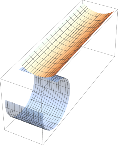
Figure 2. Plot of minimal energy configurations for the free-energy functional $\mathscr{E}^{lim}_{T}$ defined in (3.29), arising from a twisted texture of the nematic director. Under zero loads, the system is stable in each of the two configurations, hence bistable.

In the case of splay-bend textures, the curvature giving minimal energy can be predicted by simply reading it off from the target curvature tensor of the two-dimensional model (3.24) and therefore only deformations of type (4.4) with $k=12\delta_{0}/\pi^{2}$ (a portion of a cylinder with axis parallel to the image through $y$ of the line spanned by $\mathsf{e}_{2}$, and with radius $\pi^{2}/(12\delta_{0})$) are minimal energy states. This means that Gaussian curvature is suppressed in the splay-bend as well as in the twisted case, in the sense that the configurations exhibited by elastomer thin sheets in the absence of applied loads will be portions of cylindrical surfaces (with zero Gaussian curvature, as predicted in [35, 36] and observed experimentally in [30, 31, 34]). In both cases, these configurations carry non-zero residual stresses. In the twisted case, there will be also non-zero residual internal bending moments, due to the additional frustration caused by the non-attainability of the target curvature. In the splay-bend case the target curvature is attained, the bending energy is minimised to zero, and no residual moments arise.

It is worth comparing the case of twist and splay-bend textures with a different scenario, in which the nematic director is kept constant along the thickness of the thin sheet, whereas the spontaneous strain (2.2) varies along the thickness through the magnitude parameter $a$. To the best of our knowledge, a system with these features has not yet been synthesized in a laboratory. At least in principle, this should be possible by realising a film with uniform alignment of the director perpendicular to the mid-suface (direction $\mathsf{e}_{3}$), and variable degree of order along the thickness ($x_{3}$ coordinate).

Using the notation of Subsection 2.1, let us suppose that the nematic director $n^{h}(z_{3})$ is now constant, and equal to some $\mathsf{n}\in\mathbb{S}^{2}$, and that the (constant) parameter $a_{h}$ in (2.4) is now given by

$$\bar{a}_{h}(z_{3})\,:=\,1+\frac{\alpha_{0}}{h_{0}}z_{3},\qquad\qquad z_{3}\in(-h/2,h/2).$$

The (physical) spontaneous strain of this system is therefore defined as

$$\bar{c}_{h}(z_{3})\,:=\,\bar{a}_{h}^{2/3}(z_{3})\,\mathsf{n}\otimes\mathsf{n}+\bar{a}_{h}^{-1/3}(z_{3})\big{(}{\rm I}-\mathsf{n}\otimes\mathsf{n}\big{)}.$$

Modelling the system using again the prototypical energy density (2.5), as in Subsection 3.1 we can define the rescaled energy densities $W_{h}(x_{3},\cdot)$, $x_{3}\in(-1/2,1/2)$, characterised by the (rescaled) spontaneous strains

$$\overline{C}_{h}(x_{3})\,:=\,\bar{c}_{h}(hx_{3}) \,=\,\Big{(}1+\frac{\alpha_{0}}{h_{0}}h\,x_{3}\Big{)}^{2/3}\!\mathsf{n}\otimes\mathsf{n}+\Big{(}1+\frac{\alpha_{0}}{h_{0}}h\,x_{3}\Big{)}^{-1/3}\big{(}{\rm I}-\mathsf{n}\otimes\mathsf{n}\big{)}$$

$$\,=\,{\rm I}-2\,h\,B(x_{3})+R^{h}(x_{3}),\qquad\quad B(x_{3})\,:=\,\frac{x_{3}}{2}\frac{\alpha_{0}}{h_{0}}\left(\frac{\rm I}{3}-\mathsf{n}\otimes\mathsf{n}\right),$$

where $\|R^{h}\|_{\infty}=o(h)$. Proceeding as in Subsection 3.3, we obtain a limit 2D model whose free-energy functional is given by

$$\mathscr{E}^{lim}(y)\,=\,\frac{1}{2}\int\limits_{\omega}\overline{Q}_{2}(A_{y}(x^{\prime})){\rm d}x^{\prime}\,=\,\frac{1}{24}\int\limits_{\omega}Q_{2}\left(A_{y}(x^{\prime})-\check{M}\right){\rm d}x^{\prime},$$ (4.7)

for every $y\in\mathcal{A}_{iso}$. Here, the $2{\times}2$ symmetric matrix $\check{M}$ is given by the formula

$$\check{M}\,=\,\frac{1}{2}\frac{\alpha_{0}}{h_{0}}\left[(\mathsf{n}\otimes\mathsf{n})^{\check{}}-\frac{{\rm I}_{2}}{3}\right],$$

and $(\mathsf{n}\otimes\mathsf{n})^{\check{}}$ is the $2{\times}2$ upper left part of $\mathsf{n}\otimes\mathsf{n}$. In the case where $\mathsf{n}=\mathsf{e}_{3}$, the spontaneous curvature tensor $\check{M}$ reduces to

$$\check{M}\,=\,\left(\begin{array}[]{ccc}m_{0}&0\\ 0&m_{0}\end{array}\right),\qquad\qquad m_{0}\,:=\,-\frac{\alpha_{0}}{6h_{0}}.$$ (4.8)

Note that the Gaussian curvature associated with $\check{M}$ is positive. However, as for the twisted case, where the spontaneous Gaussian curvature is negative, the observable minimal energy configurations will always exhibit zero Gaussian curvature (see Lemma 3.8), because of the isometry constraint they are subjected to. More precisely, some calculations show that every isometric deformation $\bar{y}\in\mathcal{A}_{iso}$ such that $A_{\bar{y}}\equiv\bar{A}_{+}(s)$ or $A_{\bar{y}}\equiv\bar{A}_{-}(s)$ for some $s\in[-\bar{k}/2,\bar{k}/2]$, with

$$\bar{A}_{\pm}(s)\,:=\,\left(\begin{array}[]{ccc}\frac{\bar{k}\pm\sqrt{\bar{k}^{2}-4s^{2}}}{2}&s\\ s&\frac{\bar{k}\mp\sqrt{\bar{k}^{2}-4s^{2}}}{2}\end{array}\right)\!,\qquad\qquad\quad\bar{k}\,:=\,m_{0}\Big{(}\frac{1+2\gamma}{1+\gamma}\Big{)},$$ (4.9)

is such that

$$\mathscr{E}^{lim}(\bar{y})\,=\,\min\mathscr{E}^{lim}\,=\,\frac{\mu}{12}\,m_{0}^{2}\,\Big{(}\frac{1+2\gamma}{1+\gamma}\Big{)}|\omega|,$$

where the expression of $\gamma$ in terms of the 3D parameters is given in formula (3.20). Note that $\bar{A}_{-}(-\bar{k}/2)=\bar{A}_{+}(-\bar{k}/2)$ and $\bar{A}_{-}(\bar{k}/2)=\bar{A}_{+}(\bar{k}/2)$, whereas $\bar{A}_{-}(s_{1})\neq\bar{A}_{+}(s_{2})$ for every $s_{1},s_{2}\in(-\bar{k}/2,\bar{k}/2)$. Note also that the eigenvalues of $\bar{A}_{+}(s)$ and $\bar{A}_{-}(s)$ are always $\bar{k}$ and $0$ for every $s\in[-\bar{k}/2,\bar{k}/2]$, and that

$$\bar{A}_{+}(s)\,=\,R_{+}(s)\left(\begin{array}[]{ccc}\bar{k}&0\\ 0&0\end{array}\right)R_{+}(s)^{T},\qquad\qquad\bar{A}_{-}(s)\,=\,R_{-}(s)\left(\begin{array}[]{ccc}0&0\\ 0&\bar{k}\end{array}\right)R_{-}(s)^{T},$$ (4.10)

where the columns of the rotation matrices $R_{+}(s)$ and $R_{-}(s)$ are the eigenvectors corresponding to $\bar{k}$ and $0$ and to $0$ and $\bar{k}$, respectively. The explicit expressions of $R_{+}(s)$ and $R_{-}(s)$ are the following:

$$R_{\pm}(s)\,=\,\sqrt{\frac{\bar{k}+\sqrt{\bar{k}^{2}-4s^{2}}}{2\bar{k}}}\left(\begin{array}[]{ccc}1&\mp\frac{2s}{\bar{k}+\sqrt{\bar{k}^{2}-4s^{2}}}\\ \pm\frac{2s}{\bar{k}+\sqrt{\bar{k}^{2}-4s^{2}}}&1\end{array}\right)\!,$$ (4.11)

In particular, for $\bar{A}_{+}$, the directions corresponding to the eigenvalue $0$ are given, respectively, by the vector $(1,1)$ in the case $s=-\bar{k}/2$, by $(0,1)$ in the case $s=0$, and by $(1,-1)$ in the case $s=\bar{k}/2$. For $\bar{A}_{s}$, the directions corresponding to the eigenvalue $0$ are given, respectively, by the vector $(1,1)$ in the case $s=-\bar{k}/2$, by $(1,0)$ in the case $s=0$, and by $(1,-1)$ in the case $s=\bar{k}/2$. Therefore, through the matrices $\bar{A}_{+}$ and $\bar{A}_{-}$ all the possible directions corresponding to the eigenvalue $0$ (and in turn all the corresponding orthogonal eigenspaces corresponding to the eigenvector $\bar{k}$) are represented. All in all, we have that

$$\mathscr{A}\,:=\,\left\{\bar{A}_{+}(s):s\in\left[-\frac{\bar{k}}{2},\frac{\bar{k}}{2}\right]\right\}\cup\left\{\bar{A}_{-}(s):s\in\left[-\frac{\bar{k}}{2},\frac{\bar{k}}{2}\right]\right\}\,=\,\Big{\{}R\,{\rm diag}(\bar{k},0)\,R^{T}:R\in{\rm SO}(2)\Big{\}}$$

From the discussion leading to expression (4.3), we have that, given $\bar{\rho}>0$, the deformation defined as

$$y(x_{1},x_{2})\,:=\,\left(\bar{\rho}\sin\Big{(}\frac{x_{1}}{\bar{\rho}}\Big{)},x_{2},\bar{\rho}\cos\Big{(}\frac{x_{1}}{\bar{\rho}}\Big{)}\right)^{T}$$

is an isometry such that $A_{y}\equiv{\rm diag}(1/\bar{\rho},0)$. Moreover, we have that

$$y(0,0)\,=\,(0,0,\bar{\rho})^{T},\qquad\qquad\nabla y(0,0)=(\mathsf{e}_{1}|\mathsf{e}_{2}).$$ (4.12)

Consider the rotation matrices

$$R_{\alpha}\,:=\,\left(\begin{array}[]{ccc}\sin\alpha&-\cos\alpha&0\\ \cos\alpha&\sin\alpha&0\\ 0&0&1\end{array}\right),\qquad\qquad\check{R}_{\alpha}\,:=\,\left(\begin{array}[]{cc}\sin\alpha&-\cos\alpha\\ \cos\alpha&\sin\alpha\end{array}\right),$$

and note that $\check{R}_{\alpha}$ is a $(\pi/2-\alpha)$-counterclockwise rotation taking the vector $(\cos\alpha,\sin\alpha)^{T}$ into $(0,1)^{T}$. Now, setting $\bar{\rho}=1/\bar{k}$, where $\bar{k}$ is defined as in (4.9), we define the deformation

$$y^{\alpha}(x^{\prime})\,:=\,R_{\alpha}^{T}\,\circ\,y\,\circ\,\check{R}_{\alpha}(x^{\prime})\,=\,\left(\begin{array}[]{c}\bar{\rho}\sin\alpha\sin\Big{(}\frac{x_{1}\sin\alpha-x_{2}\cos\alpha}{\bar{\rho}}\Big{)}+\cos\alpha(x_{1}\cos\alpha+x_{2}\sin\alpha)\\ -\bar{\rho}\cos\alpha\sin\Big{(}\frac{x_{1}\sin\alpha-x_{2}\cos\alpha}{\bar{\rho}}\Big{)}+\sin\alpha(x_{1}\cos\alpha+x_{2}\sin\alpha)\\ \bar{\rho}\cos\alpha\cos\Big{(}\frac{x_{1}\sin\alpha-x_{2}\cos\alpha}{\bar{\rho}}\Big{)}\end{array}\right).$$ (4.13)

Simple computations show that $y^{\alpha}\in\mathcal{A}_{iso}$ and that, setting $\nu^{\alpha}:=\partial_{1}y^{\alpha}\wedge\partial_{2}y^{\alpha}$,

$$A_{y^{\alpha}}(x^{\prime})\,:=\,(\nabla^{\prime}y^{\alpha}(x^{\prime}))^{T}\nabla^{\prime}\nu^{\alpha}(x^{\prime})\,=\,\check{R}_{\alpha}^{T}\,A_{y}(\check{R}_{\alpha}x^{\prime})\,\check{R}_{\alpha}\,=\,\check{R}_{\alpha}^{T}\left(\begin{array}[]{ccc}\frac{1}{\bar{\rho}}&0\\ 0&0\end{array}\right)\check{R}_{\alpha}\,\in\,\mathscr{A}.$$

Therefore, we have that $A_{y^{\alpha}}\equiv\bar{A}_{+}(s)$ for some $s\in[-\bar{k}/2,\bar{k}/2]$ and $\alpha\mapsto y^{\alpha}$ is a continuous family of deformations minimising $\mathscr{E}^{lim}$. Note also that $y^{\alpha}$ satisfies the normalizing conditions (4.12), for every $\alpha$. Figure 3 shows minimal energy deformed configurations obtained from the family $\alpha\mapsto y^{\alpha}$.

The existence of a continuous family of deformations with (constant) minimal energy shows that a nematic elastomer sheet with constant director (perpendicular to the mid-surface) and thickness-dependent magnitude of the spontaneous strain (this can be realised by varying the degree of the nematic order along the thickness) realises a “zero-stiffness” structure in the sense of [19]. These are structures that can undergo large elastic deformations without requiring external work. Figure 3 show that the nematic sheet can accomodate any level of twisting with negligible elastic energy in between two extreme states ($\alpha=0$ and $\alpha=\pi/2$). Of course, zero-stiffness is an idealisation and, in a real system, effects that have not been taken into account in the model will lead to small, but non-zero loads in order to change shape. In the example of Sharon [23], edge effects cause energy storage which scales as $h^{7/2}$. This is a higher scaling (with smaller stored energy in the thin film limit $h\to 0$) with respect to the bending one ($h^{3}$) that our dimensionally reduced theory is designed to resolve. As a consequence, the observed response is much “softer” than the one expected from the bending stiffness of a sheet.

By contrast, sheets with twist texture are “bistable” in the sense of [20]: they exhibit two distinct possible stable shapes in the absence of loads (see Figure 2). Splay-bend sheets have only one shape minimising the energy under zero loads.

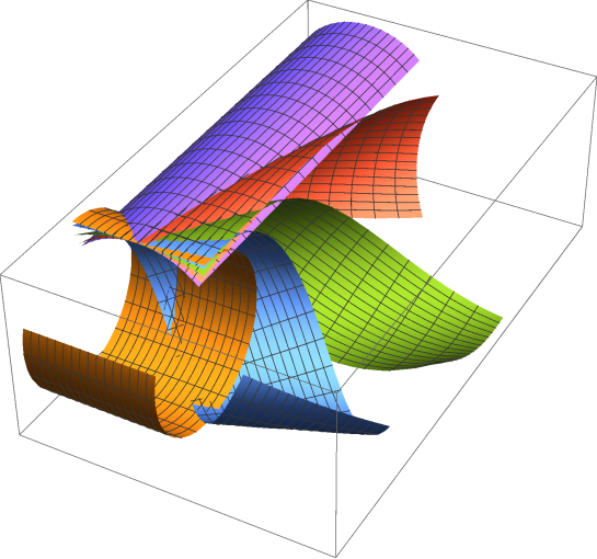
Figure 3. Plot of minimal energy configurations for the free-energy functional $\mathscr{E}^{lim}$ defined in (4.7)–(4.8), arising from constant director $\mathsf{e}_{3}$ along the thickness of the sheet. The configurations are elements of the continuous family of deformations (4.13). Under zero loads, the system has the same (minimal) energy in each of these configurations, hence it realises a structure with zero-stiffness to twisting.

Acknowledgements

We gratefully acknowledge the support by the European Research Council through the ERC Advanced Grant 340685-MicroMotility. We thank S. Guest, R. V. Kohn, and E. Sharon for valuable discussions.

References

- [1] V. Agostiniani and A. DeSimone. -convergence of energies for nematic elastomers in the small strain limit. Contin. Mech. Thermodyn., 23(3):257–274, 2011.
- [2] V. Agostiniani and A. DeSimone. Ogden-type energies for nematic elastomers. International Journal of Non-Linear Mechanics, 47(2):402 – 412, 2012.
- [3] H. Aharoni, E. Sharon, and R. Kupferman. Geometry of thin nematic elastomer sheets. Phys. Rev. Lett., 113:257801, Dec 2014.
- [4] M. Arroyo and A. DeSimone. Shape control of active surfaces inspired by the movement of euglenids. Journal of the Mechanics and Physics of Solids, 62:99–112, 2014.
- [5] M. Arroyo, L. Heltai, D. Millan, and A. DeSimone. Reverse engineering the euglenoid movement. Proceedings of the National Academy of Sciences, 109(44):17874–17879, October 2012.
- [6] M. Barchiesi and A. DeSimone. Frank energy for nematic elastomers: a nonlinear model. ESAIM-COCV, 21(2):372–377, 2015.
- [7] S. Bartels, A. Bonito, and R. H. Nochetto. Bilayer plates: model reduction, -convergent finite element approximation, and discrete gradient flow. Communications on Pure and Applied Mathematics, 2015.
- [8] K. Bhattacharya, M. Lewicka, and M. Schäffner. Plates with incompatible prestrain. Archive for Rational Mechanics and Analysis, 221(1):143–181, 2016.
- [9] P. Bladon, E. M. Terentjev, and M. Warner. Transitions and instabilities in liquid crystal elastomers. Phys. Rev. E, 47:R3838–R3840, Jun 1993.
- [10] P. Cesana and A. DeSimone. Quasiconvex envelopes of energies for nematic elastomers in the small strain regime and applications. J. Mech. Phys. Solids, 59(4):787–803, 2011.
- [11] P.G. Ciarlet. An Introduction to Differential Geometry with Applications to Elasticity. Available online. Springer, 2006.
- [12] S. Conti, A. DeSimone, and G. Dolzmann. Soft elastic response of stretched sheets of nematic elastomers: a numerical study. J. Mech. Phys. Solids, 50(7):1431–1451, 2002.
- [13] A. DeSimone. Energetics of fine domain structures. Ferroelectrics, 222(1–4):275–284, 1999.
- [14] A. DeSimone and G. Dolzmann. Macroscopic response of nematic elastomers via relaxation of a class of -invariant energies. Arch. Ration. Mech. Anal., 161(3):181–204, 2002.
- [15] A. DeSimone and L. Teresi. Elastic energies for nematic elastomers. The European Physical Journal E, 29(2):191–204, 2009.
- [16] P.J. Flory. Principles of Polymer Chemistry. Baker lectures 1948. Cornell University Press, 1953.
- [17] G. Friesecke, R. D. James, and S. Müller. A theorem on geometric rigidity and the derivation of nonlinear plate theory from three-dimensional elasticity. Comm. Pure Appl. Math., 55(11):1461–1506, 2002.
- [18] A. Fukunaga, K. Urayama, T. Takigawa, A. DeSimone, and L. Teresi. Dynamics of electro-opto-mechanical effects in swollen nematic elastomers. Macromolecules, 41(23):9389–9396, 2008.
- [19] S. D. Guest, E. Kebadze, and S. Pellegrino. A zero–stiffness elastic shell structure. Journal of Mechanics of Materials and Structures, 6(1–4):203–212, 2011.
- [20] S. D. Guest and S. Pellegrino. Analytical models for bistable cylindrical shells. Proceedings of the Royal Society A, 462:839–854, 2006.
- [21] L.H. He. Response of constrained glassy splay-bend and twist nematic sheets to light and heat. The European Physical Journal E, 36(8), 2013.
- [22] Y. Klein, E Efrati, and E Sharon. Shaping of elastic sheets by prescription of non-euclidean metrics. Science, 315(5815):1116–1120, 2007.
- [23] I. Levin and E. Sharon. Anomalously soft non-euclidean springs. Phys. Rev. Lett., 116:035502, Jan 2016.
- [24] M. Lewicka and R. Pakzad. Scaling laws for non-Euclidean plates and the isometric immersions of Riemannian metrics. ESAIM: Control Optim. Calc. Var, 17(4):1158–1173, 11 2011.
- [25] Alessandro Lucantonio and Antonio DeSimone. Computational design of shape-programmable gel plates. Journal of Computational Physics, page submitted, 2017.
- [26] C. D. Modes, K. Bhattacharya, and M. Warner. Gaussian curvature from flat elastica sheets. Proc. Roy. Soc. A, 467(2128):1121–1140, 2011.
- [27] C. D. Modes and M. Warner. Negative Gaussian curvature from induced metric changes. Phys. Rev. E, 92:010401, Jul 2015.
- [28] C. Mostajeran. Curvature generation in nematic surfaces. Phys. Rev. E, 91:062405, Jun 2015.
- [29] L. M. Pismen. Metric theory of nematoelastic shells. Phys. Rev. E, 90:060501, Dec 2014.
- [30] Y. Sawa, K. Urayama, T. Takigawa, A. DeSimone, and L. Teresi. Thermally driven giant bending of liquid crystal elastomer films with hybrid alignment. Macromolecules, 43:4362–4369, May 2010.
- [31] Y. Sawa, F. Ye, K. Urayama, T. Takigawa, V. Gimenez-Pinto, R. L. B. Selinger, and J. V. Selinger. Shape selection of twist-nematic-elastomer ribbons. PNAS, 108(16):6364–6368, 2011.
- [32] B. Schmidt. Plate theory for stressed heterogeneous multilayers of finite bending energy. J. Math. Pures Appl., 88(1):107 – 122, 2007.
- [33] A. Shahaf, E. Efrati, R. Kupferman, and E. Sharon. Geometry and mechanics in the opening of chiral seed pods. Science, 333(6050):1726–1730, 2011.
- [34] K. Urayama. Switching shapes of nematic elastomers with various director configurations. Reactive and Functional Polymers, 73(7):885–890, 2013. Challenges and Emerging Technologies in the Polymer Gels.
- [35] M. Warner, C. D. Modes, and D. Corbett. Curvature in nematic elastica responding to light and heat. Proceedings of the Royal Society of London A: Mathematical, Physical and Engineering Sciences, 466(2122):2975–2989, 2010.
- [36] M. Warner, C. D. Modes, and D. Corbett. Suppression of curvature in nematic elastica. Proc. R. Soc. A, pages 3561–3578, 2010.