An integrable semi-discretization of the coupled Yajima–Oikawa system

Abstract

In the present paper, an integrable semi-discrete analogue of the one-dimensional coupled Yajima–Oikawa system, which is comprised of multicomponent short-wave and one component long-wave, is proposed by using Hirota’s bilinear method. Based on the reductions of the Bäcklund transformations of the semi-discrete BKP hierarchy, both the bright and dark soliton (for the short-wave components) solutions in terms of pfaffians are constructed.

1 Introduction

Both the nonlinear Schrödinger (NLS) equation and the Yajima-Oikawa (YO) equation are import models arising in a variety of physical contexts [1]. It is known that they can be derived from the so-called $k$-constrained KP hierarchy [2]. Specifically, the NLS equation corresponds to the $k$-constrained KP hierarchy with $k=1$, while the YO equation is associated with the case with $k=2$ [3].

The integrable discretization of nonlinear Schrödinger equation

$$\mathrm{i}q_{n,t}=\left(1+\sigma|q_{n}|^{2}\right)\left(q_{n+1}+q_{n-1}\right)\,$$ (1)

was originally derived by Ablowitz and Ladik [35, 36], and was named Ablowatiz-Ladik (AL) lattice. Similar to the continuous case, the AL lattice equation admits bright soliton solution for the focusing case ($\sigma=1$) [4, 5] and dark soliton solution for the defocusing case ($\sigma=-1)$ [6]. The geometric construction of the AL lattice was given by Doliwa and Santini [7].

The semi-discrete coupled nonlinear Schrödinger equation

$$\mathrm{i}q_{n,t}^{(1)} = \left(1+\sigma_{1}|q_{n}^{(1)}|^{2}+\sigma_{2}|q_{n}^{(2)}|^{2}\right)\left(q_{n+1}^{(1)}+q_{n-1}^{(1)}\right)\,,$$ (2)

$$\mathrm{i}q_{n,t}^{(2)} = \left(1+\sigma_{1}|q_{n}^{(1)}|^{2}+\sigma_{2}|q_{n}^{(2)}|^{2}\right)\left(q_{n+1}^{(2)}+q_{n-1}^{(2)}\right)$$ (3)

where $\sigma_{i}=\pm 1(i=1,2)$, is of importance both mathematically and physically. It was solve by the inverse scattering method in [8, 9]. The general multi-soliton solution in terms of pfaffians was found recently in [10, 11], which is of bright type for the focusing-focusing case ($\sigma_{1}=\sigma_{2}=1$), is of dark type for the defocusing-defocusing case ($\sigma_{1}=\sigma_{2}=-1$), and could be of mixed type for the focusing-defocusing case ($\sigma_{1}=1$, $\sigma_{2}=-1$).

In compared with the successful construction of the integrable discrete analogue of the NLS equation and the coupled NLS equations, the integrable discrete analogues of the YO equation and its multi-component generalizations are missing. It should be pointed out that fully discrete NLS and YO equations were constructed most recently [12], however, their semi-discrete limits cannot converge to the model such as the Ablowatiz-Ladik lattice. Therefore, it is of important to construct an integrable semi-discrete analogue of the one-dimensional (1D) coupled Yajima-Oikawa (YO) system:

$${\rm i}S^{(\mu)}_{t}-S^{(\mu)}_{xx}-LS^{(\mu)}=0,\ \ \mu=1,2,\cdots,M,$$ (4)

$$L_{t}=2\sum^{M}_{\mu=1}c^{(\mu)}(|S^{(\mu)}|^{2})_{x},$$ (5)

where $c^{(\mu)}$ are arbitrary real constants, $S^{(\mu)}$ and $L$ indicate the $\mu$th short-wave (SW) and long-wave (LW) components, respectively.

When $M=1$, the original YO system described such a physical process, in which a resonant interaction takes place between a weakly dispersive LW and a SW packet when the phase velocity of the former exactly or almost matches the group velocity of the latter [14]. Yajima and Oikawa [15] proposed the model equation for the interaction of a Langmuir wave with an ion-acoustic wave in a plasma and showed that the system is integrable by the inverse scattering transform method. This model equation was also derived in diverse physical backgrounds such as hydrodynamics [16], nonlinear optics [17, 18] and biophysics [19]. It admits both bright and dark soliton solutions [20, 21, 22]. The rogue wave solutions to the 1D YO system have recently been derived by using Hirota’s bilinear method [23] and Darboux transformation [24]. For the multicomponent 1D YO system (4)-(5), it can be obtained from the KP-hierarchy by reduction as shown in Ref. [25, 26, 27]. Most recently, Kanna et al. [28] considered the multicomponent coupled 1D YO system (4)-(5), and pointed out that the coupled YO system with two component LWs ($M=2$) can be deduced from a set of three coupled NLS equations governing the propagation of three optical fields in a triple mode optical fiber by applying the asymptotic reduction procedure [28]. Eqs.(4)-(5) has also been derived to describe the interaction between a quasi-resonance circularly polarized optical pulse and a long-wave electromagnetic spike [29]. In the context of many-component magnon-phonon system, such a multicomponent YO system has also been proposed and its corresponding Hamiltonian formalism was studied [30]. Also, the authors in ref.[28] have carried out Painlevé analysis for Eqs.(4)-(5) and obtained the general bright N-soliton solution in the Gram determinant form. Soon after, they constructed an extensive set of exact periodic solutions in terms of Lamé polynomials of order one and two [31]. With the help of the KP-hierarchy reduction method, we have recently considered the dark soliton, mixed soliton and rational solutions for the coupled YO system (4)-(5) in [32, 33, 34].

Integrable discretizations of integrable systems have received considerable attention recently (see, e.g., [13] and references therein). So far, several approaches have been developed to construct integrable difference analogues of soliton equations. Ablowitz and Ladik proposed a method of integrable discretization by using Lax pairs [35, 36]. Based on the bilinear form, Hirota developed a method to construct integrable discrete analogues of soliton equations [37, 38, 39]. Date et al [40, 41, 42, 43, 44] have shown an effective way to discretize integrable equations via the transformation group theory, in which many of discretization versions of soliton equations can be derived by reduction. Suris [45] also developed a general Hamiltonian approach for integrable discretizations of soliton equations. In a series of recent research, the bilinear integrable discretization method has been widely applied to construct discrete schemes of the coupled Nonlinear Schrödinger equation [10, 11], the (2+1)-dimensional sinh-Gordon equation [46], the two–dimensional Leznov lattice equation [47], the Camassa–Holm equation [48, 49], the short pulse equation [50] and coupled short pulse equation [51, 52], the short-wave model of the Camassa–Holm equation [53], the reduced Ostrovsky equation [54], the coupled integrable dispersionless equation [55], the integrable (2+1)-dimensional Zakharov equation [56] and so on.

The goal of the present paper is to construct an integrable semi-discrete analogue of the coupled YO system by virtue of Hirota’s bilinear method, and derive both the bright and dark soliton (for the SW components) solutions by the KP-hierarchy reduction method. The remainder of the paper is organized as follows. In section 2, we present an integrable semi-discrete version of the coupled YO system. In section 3 and 4, the bright and dark soliton solutions in terms of pfaffians of the semi-discrete coupled YO system are constructed based on two types of Bäcklund transformation of the BKP hierarchy. Section 5 is concluded by some comments and discussions.

2 Integrable semi-discrete coupled YO system

Through the dependent variable transformation

$$S^{(\mu)}=\frac{G^{(\mu)}}{F},\ \ L=2(\ln F)_{xx},\ \ \mu=1,2,\cdots,M,$$ (6)

the 1D coupled YO equations (4)-(5) can be cast into the bilinear form

$$({\rm i}D_{t}-D^{2}_{x})G^{(\mu)}\cdot F=0,\ \ \mu=1,2,\cdots,M,$$ (7)

$$D_{x}D_{t}F\cdot F-2cF\cdot F=2\sum^{M}_{\mu=1}c^{(\mu)}G^{(\mu)}\bar{G}^{(\mu)},$$ (8)

where $c$ is an integral constant and $\bar{}$ means complex conjugate. The Hirota’s bilinear differential operator is defined by

$$D^{n}_{x}D^{m}_{t}(a\cdot b)=\bigg{(}\frac{\partial}{\partial x}-\frac{\partial}{\partial x^{\prime}}\bigg{)}^{n}\bigg{(}\frac{\partial}{\partial t}-\frac{\partial}{\partial t^{\prime}}\bigg{)}^{m}a(x,t)b(x^{\prime},t^{\prime})\bigg{|}_{x=x^{\prime},t=t^{\prime}}.$$

By discretizing the spacial part of the above bilinear equations,

$$D^{2}_{x}G^{(\mu)}\cdot F\rightarrow\frac{1}{\epsilon^{2}}(G^{(\mu)}_{n+1}F_{n-1}-2G^{(\mu)}_{n}F_{n}+G^{(\mu)}_{n-1}F_{n+1}),$$ (9)

$$F_{x}=\frac{1}{\epsilon}(F_{n+1}-F_{n}),$$ (10)

one can obtain

$${\rm i}D_{t}G^{(\mu)}_{n}\cdot F_{n}-\frac{1}{\epsilon^{2}}(G^{(\mu)}_{n+1}F_{n-1}-2G^{(\mu)}_{n}F_{n}+G^{(\mu)}_{n-1}F_{n+1})=0,\ \ \mu=1,2,\cdots,M,$$ (11)

$$\frac{1}{\epsilon}D_{t}F_{n+1}\cdot F_{n}-cF_{n}\cdot F_{n}=\sum^{M}_{\mu=1}c^{(\mu)}G^{(\mu)}_{n}\bar{G}^{(\mu)}_{n}.$$ (12)

Furthermore, we require that the discretized bilinear forms are invariant under the gauge transformation

$$F_{n}\rightarrow F_{n}\exp(q_{0}n),\ \ G^{(\mu)}_{n}\rightarrow G^{(\mu)}_{n}\exp(q_{0}n),$$

then one gets the gauge invariant semi-discrete bilinear YO equations

$${\rm i}D_{t}G^{(\mu)}_{n}\cdot F_{n}-\frac{1}{\epsilon^{2}}(G^{(\mu)}_{n+1}F_{n-1}-2G^{(\mu)}_{n}F_{n}+G^{(\mu)}_{n-1}F_{n+1})=0,\ \ \mu=1,2,\cdots,M,$$ (13)

$$\frac{1}{\epsilon}D_{t}F_{n+1}\cdot F_{n}-cF_{n+1}\cdot F_{n}=\sum^{M}_{\mu=1}\frac{c^{(\mu)}}{2}(G^{(\mu)}_{n+1}\bar{G}^{(\mu)}_{n}+G^{(\mu)}_{n}\bar{G}^{(\mu)}_{n+1}).$$ (14)

Let

$$S^{(\mu)}_{n}=\frac{G^{(\mu)}_{n}}{F_{n}},\ \ L_{n}=\frac{2}{\epsilon^{2}}\left(\frac{F_{n+1}F_{n-1}}{F^{2}_{n}}-1\right),\ \ \hat{\hat{L}}_{n}=2\ln F_{n},$$ (15)

the bilinear equations (13)-(14) are transformed into

$${\rm i}\frac{d}{dt}S^{(\mu)}_{n}-\frac{1}{\epsilon^{2}}(S^{(\mu)}_{n+1}+S^{(\mu)}_{n-1}-2S^{(\mu)}_{n})-\frac{1}{2}L_{n}(S^{(\mu)}_{n+1}+S^{(\mu)}_{n-1})=0,\ \ \mu=1,2,\cdots,M,$$ (16)

$$\frac{1}{\epsilon}(\hat{\hat{L}}_{n+1,t}-\hat{\hat{L}}_{n,t})-2c=\sum^{M}_{\mu=1}c^{(\mu)}(S^{(\mu)}_{n+1}\bar{S}^{(\mu)}_{n}+S^{(\mu)}_{n}\bar{S}^{(\mu)}_{n+1}).$$ (17)

By using the relation $\frac{1}{2}(\hat{\hat{L}}_{n+1}-2\hat{\hat{L}}_{n}+\hat{\hat{L}}_{n-1})=\ln(1+\frac{\epsilon^{2}}{2}L_{n})$, we propose the following discrete system

$${\rm i}\frac{d}{dt}S^{(\mu)}_{n}-\frac{1}{\epsilon^{2}}(S^{(\mu)}_{n+1}+S^{(\mu)}_{n-1}-2S^{(\mu)}_{n})-\frac{1}{2}L_{n}(S^{(\mu)}_{n+1}+S^{(\mu)}_{n-1})=0,\ \ \mu=1,2,\cdots,M,$$ (18)

$$2\frac{d}{dt}\frac{\ln(1+\frac{\epsilon^{2}}{2}L_{n})}{\epsilon^{2}}=\sum^{M}_{\mu=1}\frac{c^{(\mu)}}{\epsilon}[(S^{(\mu)}_{n+1}-S^{(\mu)}_{n-1})\bar{S}^{(\mu)}_{n}+S^{(\mu)}_{n}(\bar{S}^{(\mu)}_{n+1}-\bar{S}^{(\mu)}_{n-1})],$$ (19)

which converges to the coupled YO system (4)-(5) when $\epsilon\rightarrow 0$.

For simplicity, by taking $\epsilon=1$ and applying the gauge transformation $S^{(\mu)}_{n}\rightarrow\exp(2{\rm i}t)S^{(\mu)}_{n}$, one can obtain the semi-discrete YO equations

$${\rm i}\frac{d}{dt}S^{(\mu)}_{n}=(S^{(\mu)}_{n+1}+S^{(\mu)}_{n-1})(1+\frac{1}{2}L_{n}),\ \ \mu=1,2,\cdots,M,$$ (20)

$$\hat{\hat{L}}_{n+1,t}-\hat{\hat{L}}_{n,t}-2c=\sum^{M}_{\mu=1}c^{(\mu)}(S^{(\mu)}_{n+1}\bar{S}^{(\mu)}_{n}+S^{(\mu)}_{n}\bar{S}^{(\mu)}_{n+1}),$$ (21)

$$\ln(1+\frac{L_{n}}{2})=\frac{1}{2}(\hat{\hat{L}}_{n+1}-2\hat{\hat{L}}_{n}+\hat{\hat{L}}_{n-1}),$$ (22)

or

$${\rm i}\frac{d}{dt}S^{(\mu)}_{n}=(S^{(\mu)}_{n+1}+S^{(\mu)}_{n-1})(1+\frac{1}{2}L_{n}),\ \ \mu=1,2,\cdots,M,$$ (23)

$$2\frac{d}{dt}\ln(1+\frac{L_{n}}{2})=\sum^{M}_{\mu=1}c^{(\mu)}[(S^{(\mu)}_{n+1}-S^{(\mu)}_{n-1})\bar{S}^{(\mu)}_{n}+S^{(\mu)}_{n}(\bar{S}^{(\mu)}_{n+1}-\bar{S}^{(\mu)}_{n-1})].$$ (24)

In the subsequent two sections, we will consider general bright and dark soliton solutions for semi-discete coupled YO system (23)-(24) in details. For brevity, we refer to the soliton solution including bright or dark soliton for the SW components and bright one for the LW component as the bright or dark soliton solution.

3 Bright soliton solution for the semi-discete coupled YO system

In this section, we will construct bright soliton solution for the semi-discete coupled YO system (23)-(24). First, we briefly recall Bäcklund transformations of the semi-discrete BKP hierarchy by the following Lemma [10].

Lemma 3.1 The following bilinear equations

$$D_{t}g^{(\mu)}_{n}\cdot f_{n}=g^{(\mu)}_{n+1}f_{n-1}-g^{(\mu)}_{n-1}f_{n+1},$$ (25)

$$D_{t}h^{(\mu)}_{n}\cdot f_{n}=h^{(\mu)}_{n+1}f_{n-1}-h^{(\mu)}_{n-1}f_{n+1},$$ (26)

$$D_{y^{(\mu)}}f_{n+1}\cdot f_{n}=g^{(\mu)}_{n+1}h^{(\mu)}_{n}-g^{(\mu)}_{n}h^{(\mu)}_{n+1},$$ (27)

for $\mu=1,\cdots,M$ are satisfied by the pfaffians

$$f_{n}={\rm pf}(a_{1},\cdots,a_{2N},c_{2N},\cdots,c_{1}),$$ (28)

$$g^{(\mu)}_{n}={\rm pf}(d_{0},a_{1},\cdots,a_{2N},c_{2N},\cdots,c_{1},\alpha^{(\mu)}),$$ (29)

$$h^{(\mu)}_{n}={\rm pf}(d_{0},a_{1},\cdots,a_{2N},c_{2N},\cdots,c_{1},\beta^{(\mu)}),$$ (30)

where the pfaffian elements are defined by

$${\rm pf}(a_{j},a_{k})=\frac{p_{j}-p_{k}}{p_{j}p_{k}-1}(p_{j}p_{k})^{n}\exp(\xi_{j}+\xi_{k}),$$

$${\rm pf}(d_{l},a_{j})=p^{n+l}_{j}\exp(\xi_{j}),\ \ {\rm pf}(a_{j},c_{k})=\delta_{jk},$$

$${\rm pf}(d_{l},c_{j})={\rm pf}(d_{l},\alpha^{(\mu)})={\rm pf}(d_{l},\beta^{(\mu)})={\rm pf}(a_{j},\alpha^{(\mu)})={\rm pf}(a_{j},\beta^{(\mu)})=0,$$

$${\rm pf}(c_{j},c_{k})=\left\{\begin{array}[]{ll}\sum^{M}_{\mu=1}\frac{\exp(\zeta^{(\mu)}_{j}+\eta^{(\mu)}_{k})}{Q^{(\mu)}_{j}+P^{(\mu)}_{k}},&2N\geq j\geq N+1,N\geq k\geq 1;\\ 0,&\hbox{otherwise,}\end{array}\right.$$

$${\rm pf}(c_{j},\alpha^{(\mu)})=\left\{\begin{array}[]{ll}\exp(\eta^{(\mu)}_{j}),&N\geq j\geq 1;\\ 0,&2N\geq j\geq N+1,\end{array}\right.$$

$${\rm pf}(c_{j},\beta^{(\mu)})=\left\{\begin{array}[]{ll}0,&N\geq j\geq 1;\\ \exp(\zeta^{(\mu)}_{j}),&2N\geq j\geq N+1,\end{array}\right.$$

with

$$\xi_{j}=(p_{j}-\frac{1}{p_{j}})t,\ \ \zeta^{(\mu)}_{j}=Q^{(\mu)}_{j}y^{(\mu)}+\zeta^{(\mu)}_{j0},\ \ \eta^{(\mu)}_{j}=P^{(\mu)}_{j}y^{(\mu)}+\eta^{(\mu)}_{j0}.$$

Here $p_{j}$, $Q^{(\mu)}_{j}$, $P^{(\mu)}_{j}$,$\zeta^{(\mu)}_{j0}$ and $\eta^{(\mu)}_{j0}$ are arbitrary constants.

Proof From the definition of the functions $f_{n}$, $g^{(\mu)}_{n}$ and $h^{(\mu)}_{n}$, we can derive the following pfaffian’s rules:

$$f_{n+1}={\rm pf}(d_{0},d_{1},\bullet),\ \ f_{n-1}={\rm pf}(d_{0},d_{-1},\bullet),\ \ \partial_{t}f_{n}={\rm pf}(d_{-1},d_{1},\bullet),$$

$$\partial_{y^{(\mu)}}f_{n}={\rm pf}(\bullet,\alpha^{(\mu)},\beta^{(\mu)}),\ \ \partial_{y^{(\mu)}}f_{n+1}={\rm pf}(d_{0},d_{1},\bullet,\alpha^{(\mu)},\beta^{(\mu)}),$$

$$g^{(\mu)}_{n+1}={\rm pf}(d_{1},\bullet,\alpha^{(\mu)}),\ \ g^{(\mu)}_{n-1}={\rm pf}(d_{-1},\bullet,\alpha^{(\mu)}),\ \ \partial_{t}g^{(\mu)}_{n}={\rm pf}(d_{0},d_{-1},d_{1},\bullet,\alpha^{(\mu)}),$$

$$h^{(\mu)}_{n+1}={\rm pf}(d_{1},\bullet,\beta^{(\mu)}),\ \ h^{(\mu)}_{n-1}={\rm pf}(d_{-1},\bullet,\beta^{(\mu)}),\ \ \partial_{t}h^{(\mu)}_{n}={\rm pf}(d_{0},d_{-1},d_{1},\bullet,\beta^{(\mu)}),$$

where

$${\rm pf}(d_{0},d_{1})={\rm pf}(d_{0},d_{-1})=1,\ \ {\rm pf}(d_{-1},d_{1})={\rm pf}(\alpha^{(\mu)},\beta^{(\mu)})=0,$$

and $(\bullet)=(a_{1},\cdots,a_{2N},c_{2N},\cdots,c_{1})$.

Now the algebraic identities of Pfaffian

$${\rm pf}(d_{0},d_{-1},d_{1},\bullet,\alpha^{(\mu)}){\rm pf}(\bullet)={\rm pf}(d_{0},d_{-1},\bullet){\rm pf}(d_{1},\bullet,\alpha^{(\mu)})$$

$$\hskip 56.9055pt-{\rm pf}(d_{0},d_{1},\bullet){\rm pf}(d_{-1},\bullet,\alpha^{(\mu)})+{\rm pf}(d_{0},\bullet,\alpha^{(\mu)}){\rm pf}(d_{-1},d_{1},\bullet),$$

$${\rm pf}(d_{0},d_{-1},d_{1},\bullet,\beta^{(\mu)}){\rm pf}(\bullet)={\rm pf}(d_{0},d_{-1},\bullet){\rm pf}(d_{1},\bullet,\beta^{(\mu)})$$

$$\hskip 56.9055pt-{\rm pf}(d_{0},d_{1},\bullet){\rm pf}(d_{-1},\bullet,\beta^{(\mu)})+{\rm pf}(d_{0},\bullet,\beta^{(\mu)}){\rm pf}(d_{-1},d_{1},\bullet),$$

and

$${\rm pf}(d_{0},d_{1},\bullet,\alpha^{(\mu)},\beta^{(\mu)}){\rm pf}(\bullet)={\rm pf}(d_{0},d_{1},\bullet){\rm pf}(\bullet,\alpha^{(\mu)},\beta^{(\mu)})$$

$$\hskip 56.9055pt-{\rm pf}(d_{0},\bullet,\alpha^{(\mu)}){\rm pf}(d_{1},\bullet,\beta^{(\mu)})+{\rm pf}(d_{1},\bullet,\alpha^{(\mu)}){\rm pf}(d_{0},\bullet,\beta^{(\mu)}),$$

together with the above Pfaffian expressions of tau functions give the bilinear equations (25)-(27). $\square$

Assume $c=0$ in Eq.(21), which implies the bright-type soliton solution for semi-discete coupled YO system. Through the dependent variable transformation

$$S^{(\mu)}_{n}={\rm i}^{n}\frac{g^{(\mu)}_{n}}{f_{n}},\ \ \bar{S}^{(\mu)}_{n}=(-{\rm i})^{n}\frac{\bar{g}^{(\mu)}_{n}}{f_{n}},\ \ L_{n}=2\left(\frac{f_{n+1}f_{n-1}}{f^{2}_{n}}-1\right),\ \ \hat{\hat{L}}=2\ln f_{n},$$ (34)

Eqs. (20)-(22) are cast into

$$D_{t}g^{(\mu)}_{n}\bullet f_{n}=g^{(\mu)}_{n+1}f_{n-1}-g^{(\mu)}_{n-1}f_{n+1},$$ (35)

$$D_{t}\bar{g}^{(\mu)}_{n}\bullet f_{n}=\bar{g}^{(\mu)}_{n+1}f_{n-1}-\bar{g}^{(\mu)}_{n-1}f_{n+1},$$ (36)

$$D_{t}f_{n+1}\bullet f_{n}=\sum^{M}_{\mu=1}{\rm i}\frac{c^{(\mu)}}{2}(g^{(\mu)}_{n+1}\bar{g}^{(\mu)}_{n}-g^{(\mu)}_{n}\bar{g}^{(\mu)}_{n+1}),$$ (37)

for $\mu=1,\cdots,M$.

In order to carry out the dimension reduction, we define

$${\rm pf}(a^{\prime}_{j},a^{\prime}_{k})=\frac{p_{j}-p_{k}}{p_{j}p_{k}-1}(p_{j}p_{k})^{n},$$

$${\rm pf}(d_{l},a^{\prime}_{j})=p^{n+l}_{j},\ \ {\rm pf}(a^{\prime}_{j},c^{\prime}_{k})=\delta_{jk},$$

$${\rm pf}(d_{l},c^{\prime}_{j})={\rm pf}(d_{l},\alpha^{(\mu)})={\rm pf}(d_{l},\beta^{(\mu)})={\rm pf}(a^{\prime}_{j},\alpha^{(\mu)})={\rm pf}(a^{\prime}_{j},\beta^{(\mu)})=0,$$

$${\rm pf}(c^{\prime}_{j},c^{\prime}_{k})=\left\{\begin{array}[]{ll}\sum^{M}_{\mu=1}\frac{\exp(\zeta^{(\mu)}_{j}+\eta^{(\mu)}_{k}+\xi_{j}+\xi_{k})}{Q^{(\mu)}_{j}+P^{(\mu)}_{k}},&2N\geq j\geq N+1,N\geq k\geq 1;\\ 0,&\hbox{otherwise,}\end{array}\right.$$

$${\rm pf}(c^{\prime}_{j},\alpha^{(\mu)})=\left\{\begin{array}[]{ll}\exp(\eta^{(\mu)}_{j}+\xi_{j}),&N\geq j\geq 1;\\ 0,&2N\geq j\geq N+1,\end{array}\right.$$

$${\rm pf}(c^{\prime}_{j},\beta^{(\mu)})=\left\{\begin{array}[]{ll}0,&N\geq j\geq 1;\\ \exp(\zeta^{(\mu)}_{j}+\xi_{j}),&2N\geq j\geq N+1.\end{array}\right.$$

Then, the Pfaffians $f_{n}$, $g_{n}^{(\mu)}$ and $h_{n}^{(\mu)}$ in Eqs.(28)-(30) have alternative expressions in pfaffians

$$f_{n}={\rm pf}(a^{\prime}_{1},\cdots,a^{\prime}_{2N},c^{\prime}_{2N},\cdots,c^{\prime}_{1}),$$ (41)

$$g^{(\mu)}_{n}={\rm pf}(d_{0},a^{\prime}_{1},\cdots,a^{\prime}_{2N},c^{\prime}_{2N},\cdots,c^{\prime}_{1},\alpha^{(\mu)}),$$ (42)

$$h^{(\mu)}_{n}={\rm pf}(d_{0},a^{\prime}_{1},\cdots,a^{\prime}_{2N},c^{\prime}_{2N},\cdots,c^{\prime}_{1},\beta^{(\mu)}).$$ (43)

Therefore, under the reduction conditions,

$$P^{(\mu)}_{j}=\frac{1}{s^{(\mu)}}(p_{j}-\frac{1}{p_{j}}),\ \ N\geq j\geq 1;\ \ Q^{(\mu)}_{j}=\frac{1}{s^{(\mu)}}(p_{j}-\frac{1}{p_{j}}),\ \ 2N\geq j\geq N+1,$$ (44)

the following relation holds

$$\partial_{t}(f_{n},g^{(\nu)}_{n},h^{(\nu)}_{n})=\sum^{M}_{\mu=1}s^{(\mu)}\partial_{y^{(\mu)}}(f_{n},g^{(\nu)}_{n},h^{(\nu)}_{n}),$$ (45)

and thus one can get

$$D_{t}f_{n+1}\cdot f_{n}=\sum^{M}_{\mu=1}s^{(\mu)}(g^{(\mu)}_{n+1}h^{(\mu)}_{n}-g^{(\mu)}_{n}h^{(\mu)}_{n+1}).$$ (46)

Lastly, by taking the complex conjugate conditions

$$s^{(\mu)}={\rm i}\frac{c^{(\mu)}}{2},\ \ p_{2N+1-j}=\bar{p}_{j},\ \ \zeta^{(\mu)}_{p_{2N+1-j,0}}=\bar{\eta}^{(\mu)}_{j,0},\ \ \mbox{for}\ \ N\geq j\geq 1,$$ (47)

and $y^{(\mu)}$ are pure imaginary, then the function $h^{(\mu)}_{n}=\bar{g}^{(\mu)}_{n}$, and Eqs.(25), (26) and (46) become Eqs.(35)–(37).

To summarize, we arrive at a Theorem below:

Theorem 3.1 The bilinear equations (35)–(37) are satisfied by the Pfaffians,

$$f_{n}={\rm pf}(a^{\prime}_{1},\cdots,a^{\prime}_{2N},c^{\prime}_{2N},\cdots,c^{\prime}_{1}),$$ (48)

$$g^{(\mu)}_{n}={\rm pf}(d_{0},a^{\prime}_{1},\cdots,a^{\prime}_{2N},c^{\prime}_{2N},\cdots,c^{\prime}_{1},\alpha^{(\mu)}),$$ (49)

$$\bar{g}^{(\mu)}_{n}={\rm pf}(d_{0},a^{\prime}_{1},\cdots,a^{\prime}_{2N},c^{\prime}_{2N},\cdots,c^{\prime}_{1},\beta^{(\mu)}),$$ (50)

where the pfaffian elements are defined by

$${\rm pf}(a^{\prime}_{j},a^{\prime}_{k})=\frac{p_{j}-p_{k}}{p_{j}p_{k}-1}(p_{j}p_{k})^{n},$$

$${\rm pf}(d_{l},a^{\prime}_{j})=p^{n+l}_{j},\ \ {\rm pf}(a^{\prime}_{j},c^{\prime}_{k})=\delta_{jk},$$

$${\rm pf}(d_{l},c^{\prime}_{j})={\rm pf}(d_{l},\alpha^{(\mu)})={\rm pf}(d_{l},\beta^{(\mu)})={\rm pf}(a^{\prime}_{j},\alpha^{(\mu)})={\rm pf}(a^{\prime}_{j},\beta^{(\mu)})=0,$$

$${\rm pf}(c^{\prime}_{j},c^{\prime}_{k})=\left\{\begin{array}[]{ll}\sum^{M}_{\mu=1}\frac{\exp(\zeta^{(\mu)}_{j}+\eta^{(\mu)}_{k}+\xi_{j}+\xi_{k})}{Q^{(\mu)}_{j}+P^{(\mu)}_{k}},&2N\geq j\geq N+1,N\geq k\geq 1;\\ 0,&\hbox{otherwise,}\end{array}\right.$$

$${\rm pf}(c^{\prime}_{j},\alpha^{(\mu)})=\left\{\begin{array}[]{ll}\exp(\eta^{(\mu)}_{j}+\xi_{j}),&N\geq j\geq 1;\\ 0,&2N\geq j\geq N+1,\end{array}\right.$$

$${\rm pf}(c^{\prime}_{j},\beta^{(\mu)})=\left\{\begin{array}[]{ll}0,&N\geq j\geq 1;\\ \exp(\zeta^{(\mu)}_{j}+\xi_{j}),&2N\geq j\geq N+1.\end{array}\right.$$

with

$$P^{(\mu)}_{j}=-{\rm i}\frac{2}{c^{(\mu)}}(p_{j}-\frac{1}{p_{j}})\ \ \mbox{for}\ \ N\geq j\geq 1;$$

$$Q^{(\mu)}_{j}=-{\rm i}\frac{2}{c^{(\mu)}}(p_{j}-\frac{1}{p_{j}})\ \ \mbox{for}\ \ 2N\geq j\geq N+1,$$

$$\xi_{j}=(p_{j}-\frac{1}{p_{j}})t,\ \ \zeta^{(\mu)}_{j}=\zeta^{(\mu)}_{j,0},\ \ \eta^{(\mu)}_{j}=\eta^{(\mu)}_{j,0},$$

and $p_{j}$, $\zeta^{(\mu)}_{j}\equiv\zeta^{(\mu)}_{j,0}$ and $\eta^{(\mu)}_{j}\equiv\eta^{(\mu)}_{j,0}$ are constants satisfying $p_{2N+1-j}=\bar{p}_{j}$, $\zeta^{(\mu)}_{2N+1-j,0}=\bar{\eta}^{(\mu)}_{j,0}$ for $N\geq j\geq 1$.

In what follows, we will illustrate one and two bright soliton solutions for $M=2$.

One-soliton solution: By taking $N=1$ in (48)-(50), we get the tau functions for the one-soliton solution

$$f_{n}=1+\frac{{\rm i}}{2}\frac{(c^{(1)}A_{1}\bar{A}_{1}+c^{(2)}B_{1}\bar{B}_{1})p_{1}\bar{p}_{1}}{(p_{1}\bar{p}_{1}-1)^{2}}\frac{p_{1}-\bar{p}_{1}}{p_{1}+\bar{p}_{1}}(p_{1}\bar{p}_{1})^{n}\exp(\xi_{1}+\bar{\xi}_{1}),$$ (54)

$$g^{(1)}_{n}=A_{1}p^{n}_{1}\exp(\xi_{1}),\ \ g^{(2)}_{n}=B_{1}p^{n}_{1}\exp(\xi_{1}),$$ (55)

where $\xi_{1}=(p_{1}-\frac{1}{p_{1}})t$, $A_{1}=\exp[\eta^{(1)}_{1,0}]$ and $B_{1}=\exp[\eta^{(2)}_{1,0}]$.

In order to avoid the singularity, the condition $\frac{{\rm i}(c^{(1)}A_{1}\bar{A}_{1}+c^{(2)}B_{1}\bar{B}_{1})(p_{1}-\bar{p}_{1})}{2(p_{1}+\bar{p}_{1})}>0$ need to be satisfied. Further, the above tau functions lead to the one-soliton solution as follows

$$S^{(1)}_{n}=\frac{A_{1}}{2}\exp({\rm i}\xi^{\prime}_{1I}-\theta_{0}){\rm sech}(\xi^{\prime}_{1R}+\theta_{0}),$$ (56)

$$S^{(2)}_{n}=\frac{B_{1}}{2}\exp({\rm i}\xi^{\prime}_{1I}-\theta_{0}){\rm sech}(\xi^{\prime}_{1R}+\theta_{0}),$$ (57)

$$L_{n}=\frac{(p_{1}\bar{p}_{1}-1)^{2}}{2p_{1}\bar{p}_{1}}{\rm sech}^{2}(\xi^{\prime}_{1R}+\theta_{0}),$$ (58)

where $\xi^{\prime}_{1}=\xi^{\prime}_{1R}+{\rm i}\xi^{\prime}_{1I}=n\ln({\rm i}p_{1})+\xi_{1}$ and $\exp(2\theta_{0})=\frac{{\rm i}}{2}\frac{(c^{(1)}A_{1}\bar{A}_{1}+c^{(2)}B_{1}\bar{B}_{1})p_{1}\bar{p}_{1}}{(p_{1}\bar{p}_{1}-1)^{2}}\frac{p_{1}-\bar{p}_{1}}{p_{1}+\bar{p}_{1}}$. The quantities $\frac{|A|}{2}\exp(-\theta_{0})$ and $\frac{|B|}{2}\exp(-\theta_{0})$ represent the amplitudes of the bright solitons in the SW components $S^{(1)}_{n}$ and $S^{(2)}_{n}$ respectively. The real quantity $\frac{(p_{1}\bar{p}_{1}-1)^{2}}{2p_{1}\bar{p}_{1}}$ denotes the amplitude of soliton in the LW component. As an example, we illustrate one-soliton in Figure 1 for the nonlinearity coefficients $(c^{(1)},c^{(2)})=(1,-1)$. The parameters are chosen as $A_{1}=1$, $B_{1}=1+{\rm i}$ and $p_{1}=1+{\rm i}$.

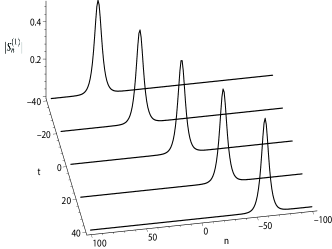
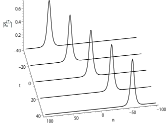
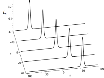
Figure 1: The profiles of evolutions of one-soliton solution (bright soliton for SW components).

Two-soliton solution: By taking $N=2$ in (48)-(50), we get the tau functions for the two-soliton solution

$$f_{n} = 1+C_{1\bar{1}}E_{1}\bar{E}_{1}+C_{1\bar{2}}E_{1}\bar{E}_{2}+C_{2\bar{1}}E_{2}\bar{E}_{1}+C_{2\bar{2}}E_{2}\bar{E}_{2},$$ (59)

$$+|P_{12}|^{2}(P_{1\bar{1}}P_{2\bar{2}}C_{1\bar{2}}C_{2\bar{1}}-P_{1\bar{2}}P_{2\bar{1}}C_{1\bar{1}}C_{2\bar{2}})E_{1}E_{2}\bar{E}_{1}\bar{E}_{2},$$

$$g^{(1)}_{n} = A_{1}E_{1}+A_{2}E_{2}+P_{12}(A_{1}P_{1\bar{1}}C_{2\bar{1}}-A_{2}P_{2\bar{1}}C_{1\bar{1}})E_{1}E_{2}\bar{E}_{1}$$ (60)

$$+P_{12}(A_{1}P_{1\bar{2}}C_{2\bar{2}}-A_{2}P_{2\bar{2}}C_{1\bar{2}})E_{1}E_{2}\bar{E}_{2},$$

$$g^{(2)}_{n} = B_{1}E_{1}+B_{2}E_{2}+P_{12}(B_{1}P_{1\bar{1}}C_{2\bar{1}}-B_{2}P_{2\bar{1}}C_{1\bar{1}})E_{1}E_{2}\bar{E}_{1}$$ (61)

$$+P_{12}(B_{1}P_{1\bar{2}}C_{2\bar{2}}-B_{2}P_{2\bar{2}}C_{1\bar{2}})E_{1}E_{2}\bar{E}_{2},$$

with

$$P_{12}=\frac{p_{1}-p_{2}}{p_{1}p_{2}-1},\ \ P_{j\bar{k}}=\frac{p_{j}-\bar{p}_{k}}{p_{j}\bar{p}_{k}-1},$$

$$E_{j}=p^{n}_{j}\exp(\xi_{j}),\ \ C_{j\bar{k}}=\frac{{\rm i}}{2}\frac{(c^{(1)}A_{j}\bar{A}_{k}+c^{(2)}B_{j}\bar{B}_{k})p_{j}\bar{p}_{k}}{(p_{j}\bar{p}_{k}-1)^{2}}\frac{p_{j}-\bar{p}_{k}}{p_{j}+\bar{p}_{k}},$$

where $\xi_{j}=(p_{j}-\frac{1}{p_{j}})t$, $A_{j}=\exp[\eta^{(1)}_{j,0}]$ and $B_{j}=\exp[\eta^{(2)}_{j,0}]$ for $j=1,2$. Figure 2 shows two-soliton interaction with the parameters as $(c^{(1)},c^{(2)})=(1,-1)$, $A_{1}=2$, $A_{2}=5$, $B_{1}=3$, $B_{2}=4$, $p_{1}=1+{\rm i}$ and $p_{2}=-\frac{1}{2}+\frac{2}{3}{\rm i}$.

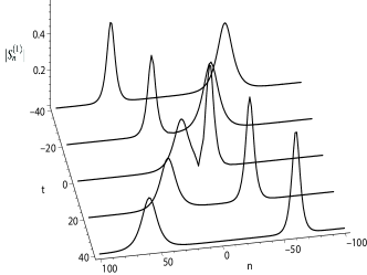
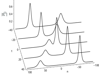
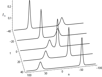
Figure 2: The profiles of evolutions of two-soliton solution (bright soliton for SW components).

4 Dark soliton solution for the semi-discete coupled YO system

In this section, we will consider dark soliton solution for the semi-discete coupled YO system (23)-(24). To this end, we need to introduce another set of Bäcklund transformations of the semi-discrete BKP hierarchy by the following Lemma [10].

Lemma 4.1 The following bilinear equations

$$(D_{t}+\alpha^{(\mu)}-\frac{1}{\alpha^{(\mu)}})g^{(\mu)}_{n}\cdot f_{n}=\alpha^{(\mu)}g^{(\mu)}_{n+1}f_{n-1}-\frac{1}{\alpha^{(\mu)}}g^{(\mu)}_{n-1}f_{n+1},$$ (62)

$$(D_{t}+\frac{1}{\alpha^{(\mu)}}-\alpha^{(\mu)})h^{(\mu)}_{n}\cdot f_{n}=\frac{1}{\alpha^{(\mu)}}h^{(\mu)}_{n+1}f_{n-1}-\alpha^{(\mu)}h^{(\mu)}_{n-1}f_{n+1},$$ (63)

$$(D_{y^{(\mu)}}-\alpha^{(\mu)}+\frac{1}{\alpha^{(\mu)}})f_{n+1}\cdot f_{n}=-\alpha^{(\mu)}g^{(\mu)}_{n+1}h^{(\mu)}_{n}+\frac{1}{\alpha^{(\mu)}}g^{(\mu)}_{n}h^{(\mu)}_{n+1},$$ (64)

for $\mu=1,\cdots,M$ are satisfied by the Pfaffians

$$f_{n}=\tau^{0\cdots 0}_{n},\ \ g_{n}^{(\mu)}=\tau_{n}^{0...\mathop{\mathop{1}\limits^{\smile}}\limits^{\mu}...0},\ \ h_{n}^{(\mu)}=\tau_{n}^{0...\mathop{\mathop{-1}\limits^{\smile}}\limits^{\mu}...0},$$ (65)

where the tau function $\tau^{l^{(1)}\cdots l^{(M)}}_{n}$ is the Pfaffian $\tau^{l^{(1)}\cdots l^{(M)}}_{n}={\rm pf}(a_{1},a_{2},\cdots,a_{2N})$, whose elements are defined by

$${\rm pf}(a_{j},a_{k})=c_{jk}+\frac{p_{j}-p_{k}}{p_{j}p_{k}-1}{\rm pf}(d_{0},a_{j}){\rm pf}(d_{0},a_{k}),$$

$${\rm pf}(d_{l},a_{j})=p^{n+l}_{j}\prod^{M}_{\mu=1}\left(\frac{p_{j}-\alpha^{(\mu)}}{1-\alpha^{(\mu)}p_{j}}\right)^{l^{(\mu)}}\exp(\xi_{j}),$$

$$\xi_{j}=(p_{j}-\frac{1}{p_{j}})t+\sum^{M}_{\mu=1}\left(\frac{p_{j}-\alpha^{(\mu)}}{1-\alpha^{(\mu)}p_{j}}-\frac{1-\alpha^{(\mu)}p_{j}}{p_{j}-\alpha^{(\mu)}}\right)y^{(\mu)}+\xi_{j,0}.$$

Proof From the definition of the tau functions, we have the following formulae of pfaffians:

$$\tau^{l^{(1)}\cdots l^{(M)}}_{n+1}={\rm pf}(d_{0},d_{1},\bullet),\ \ \tau^{l^{(1)}\cdots l^{(M)}}_{n-1}={\rm pf}(d_{0},d_{-1},\bullet),$$

$$\partial_{t}\tau^{l^{(1)}\cdots l^{(M)}}_{n}={\rm pf}(d_{-1},d_{1},\bullet),\ \ \partial_{y^{(\mu)}}\tau^{l^{(1)}\cdots l^{(M)}}_{n}={\rm pf}(d^{(\mu)}_{-1},d^{(\mu)}_{1},\bullet),$$

$$(\partial_{y^{(\mu)}}-\alpha^{(\mu)}+\frac{1}{\alpha^{(\mu)}})\tau^{l^{(1)}\cdots l^{(M)}}_{n+1}={\rm pf}(d_{0},d_{1},d^{(\mu)}_{-1},d^{(\mu)}_{1},\bullet),$$

$$\tau^{l^{(1)}\cdots l^{(\mu)}+1\cdots l^{(M)}}_{n}={\rm pf}(d_{0},d^{(\mu)}_{1},\bullet),$$

$$\alpha^{(\mu)}\tau^{l^{(1)}\cdots l^{(\mu)}+1\cdots l^{(M)}}_{n+1}={\rm pf}(d_{1},d^{(\mu)}_{1},\bullet),$$

$$\frac{1}{\alpha^{(\mu)}}\tau^{l^{(1)}\cdots l^{(\mu)}+1\cdots l^{(M)}}_{n-1}={\rm pf}(d_{-1},d^{(\mu)}_{1},\bullet),$$

$$(\partial_{t}+\alpha^{(\mu)}-\frac{1}{\alpha^{(\mu)}})\tau^{l^{(1)}\cdots l^{(\mu)}+1\cdots l^{(M)}}_{n}={\rm pf}(d_{0},d_{-1},d_{1},d^{(\mu)}_{1},\bullet),$$

$$\tau^{l^{(1)}\cdots l^{(\mu)}-1\cdots l^{(M)}}_{n}={\rm pf}(d_{0},d^{(\mu)}_{-1},\bullet),$$

$$\frac{1}{\alpha^{(\mu)}}\tau^{l^{(1)}\cdots l^{(\mu)}-1\cdots l^{(M)}}_{n+1}={\rm pf}(d_{1},d^{(\mu)}_{-1},\bullet),$$

where

$${\rm pf}(d_{0},d_{1})={\rm pf}(d_{0},d_{-1})=1,\ \ {\rm pf}(d_{-1},d_{1})=0,$$

$${\rm pf}(d^{(\mu)}_{-1},d^{(\mu)}_{1})=0,\ \ {\rm pf}(d_{0},d^{(\mu)}_{1})={\rm pf}(d_{0},d^{(\mu)}_{-1})=1,$$

$${\rm pf}(d_{1},d^{(\mu)}_{1})=\alpha^{(\mu)},\ \ {\rm pf}(d_{1},d^{(\mu)}_{-1})={\rm pf}(d_{-1},d^{(\mu)}_{1})=\frac{1}{\alpha^{(\mu)}},$$

$${\rm pf}(d^{(\mu)}_{l},a_{j})=p^{n}_{j}\left(\frac{p_{j}-\alpha^{(\mu)}}{1-\alpha^{(\mu)}p_{j}}\right)^{l}\prod^{M}_{\nu=1}\left(\frac{p_{j}-\alpha^{(\nu)}}{1-\alpha^{(\nu)}p_{j}}\right)^{l^{(\nu)}}\exp(\xi_{j}),$$

and $(\bullet)=(a_{1},\cdots,a_{2N})$.

Now the algebraic identity of pfaffians together with the previous rules for tau functions in pfaffians

$${\rm pf}(d_{0},d_{-1},d_{1},d^{(\mu)}_{1},\bullet){\rm pf}(\bullet)={\rm pf}(d_{0},d_{-1},\bullet){\rm pf}(d_{1},d_{1}^{(\mu)},\bullet)$$

$$\hskip 56.9055pt-{\rm pf}(d_{0},d_{1},\bullet){\rm pf}(d_{-1},d_{1}^{(\mu)},\bullet)+{\rm pf}(d_{0},d_{1}^{(\mu)},\bullet){\rm pf}(d_{-1},d_{1},\bullet),$$

gives the bilinear equations (62)-(63) while the algebraic identities of pfaffians

$${\rm pf}(d_{0},d_{1},d_{-1}^{(\mu)},d_{1}^{(\mu)},\bullet){\rm pf}(\bullet)={\rm pf}(d_{0},d_{1},\bullet){\rm pf}(d_{-1}^{(\mu)},d_{1}^{(\mu)},\bullet)$$

$$\hskip 56.9055pt-{\rm pf}(d_{0},d_{-1}^{(\mu)},\bullet){\rm pf}(d_{1},d_{1}^{(\mu)},\bullet)+{\rm pf}(d_{0},d_{1}^{(\mu)},\bullet){\rm pf}(d_{1},d_{-1}^{(\mu)},\bullet),$$

leads to the bilinear equation (64).$\square$

Next, we consider $c\neq 0$ in (21), which implies the dark soliton solution of the semi-discrete YO system. By applying the dependent variable transformation,

$$S^{(\mu)}_{n}=({\rm i}\alpha^{(\mu)})^{n}\exp[(\alpha^{(\mu)}-\bar{\alpha}^{(\mu)})t]\frac{g^{(\mu)}_{n}}{f_{n}},\ \ \bar{S}^{(\mu)}_{n}=(-{\rm i}\bar{\alpha}^{(\mu)})^{n}\exp[(\bar{\alpha}^{(\mu)}-\alpha^{(\mu)})t]\frac{\bar{g}^{(\mu)}_{n}}{f_{n}},$$

$$L_{n}=2\left(\frac{f_{n+1}f_{n-1}}{f^{2}_{n}}-1\right),\ \ \hat{\hat{L}}=2\ln f_{n}$$ (66)

with $|\alpha^{(\mu)}|=1$, Eqs. (20)-(22) are cast into

$$(D_{t}+\alpha^{(\mu)}-\bar{\alpha}^{(\mu)})g^{(\mu)}_{n}\bullet f_{n}=\alpha^{(\mu)}g^{(\mu)}_{n+1}f_{n-1}-\bar{\alpha}^{(\mu)}g^{(\mu)}_{n-1}f_{n+1},$$ (67)

$$(D_{t}+\bar{\alpha}^{(\mu)}-\alpha^{(\mu)})\bar{g}^{(\mu)}_{n}\bullet f_{n}=\bar{\alpha}^{(\mu)}\bar{g}^{(\mu)}_{n+1}f_{n-1}-\alpha^{(\mu)}\bar{g}^{(\mu)}_{n-1}f_{n+1},$$ (68)

$$D_{t}f_{n+1}\bullet f_{n}-cf_{n+1}\bullet f_{n}=\sum^{M}_{\mu=1}{\rm i}\frac{c^{(\mu)}}{2}(\alpha^{(\mu)}g^{(\mu)}_{n+1}\bar{g}^{(\mu)}_{n}-\bar{\alpha}^{(\mu)}g^{(\mu)}_{n}\bar{g}^{(\mu)}_{n+1}),$$ (69)

for $\mu=1,\cdots,M$.

Now we carry out the reductions to obtain bilinear equations (67)-(69) from Eqs.( 62)-(64) in Lemma 4.1. First, by taking

$$c_{jk}=\delta_{2N+1-j,k},\ \ j<k,$$ (70)

the tau functions $\tau^{l^{(1)}\cdots l^{(M)}}_{n}$ can be rewritten as

$$\tau^{l^{(1)}\cdots l^{(M)}}_{n}={\rm pf}(a^{\prime}_{1},a^{\prime}_{2},\cdots,a^{\prime}_{2N})\prod^{2N}_{j=1}{\rm pf}(d_{0},a_{j})$$ (71)

where

$${\rm pf}(a^{\prime}_{j},a^{\prime}_{k})=\delta_{2N+1-j,k}\frac{1}{{\rm pf}(d_{0},a_{j}){\rm pf}(d_{0},a_{2N+1-j})}+\frac{p_{j}-p_{k}}{p_{j}p_{k}-1},\ \ j<k.$$ (72)

Thus, if $p_{j}$ satisfies the constraint condition:

$$\sum^{M}_{\mu=1}s^{(\mu)}\left(\frac{p_{j}-\alpha^{(\mu)}}{1-\alpha^{(\mu)}p_{j}}-\frac{1-\alpha^{(\mu)}p_{j}}{p_{j}-\alpha^{(\mu)}}+\frac{p_{2N+1-j}-\alpha^{(\mu)}}{1-\alpha^{(\mu)}p_{2N+1-j}}-\frac{1-\alpha^{(\mu)}p_{2N+1-j}}{p_{2N+1-j}-\alpha^{(\mu)}}\right)$$

$$=p_{j}-\frac{1}{p_{j}}+p_{2N+1-j}-\frac{1}{p_{2N+1-j}},$$ (73)

i.e.,

$$\sum^{M}_{\mu=1}s^{(\mu)}\left(\alpha^{(\mu)}{-}\frac{1}{\alpha^{(\mu)}}\right)\left[\frac{1}{(1{-}\alpha^{(\mu)}p_{j})(1{-}\frac{1}{\alpha^{(\mu)}}p_{2N+1-j})}+\frac{1}{(1{-}\alpha^{(\mu)}p_{2N+1-j})(1{-}\frac{1}{\alpha^{(\mu)}}p_{j})}\right]$$

$$=\frac{1}{p_{j}}+\frac{1}{p_{2N+1-j}},$$ (74)

then we have

$$\partial_{t}\tau^{l^{(1)}\cdots l^{(M)}}_{n}=\sum^{M}_{\mu=1}s^{(\mu)}\partial_{y^{(\mu)}}\tau^{l^{(1)}\cdots l^{(M)}}_{n}.$$ (75)

Applying the above relation (75) to Eq. (64), we have

$$[D_{t}-\sum^{M}_{\mu=1}s^{(\mu)}(\alpha^{(\mu)}-\frac{1}{\alpha^{(\mu)}})]f_{n+1}\cdot f_{n}=-\sum^{M}_{\mu=1}s^{(\mu)}(\alpha^{(\mu)}g^{(\mu)}_{n+1}h^{(\mu)}_{n}-\frac{1}{\alpha^{(\mu)}}g^{(\mu)}_{n}h^{(\mu)}_{n+1}).$$ (76)

Furthermore, imposing the complex conjugate conditions

$$s^{(\mu)}=-{\rm i}\frac{c^{(\mu)}}{2},\ \ p_{2N+1-j}=\bar{p}_{j},\ \ \xi^{(\mu)}_{p_{2N+1-j,0}}=\bar{\xi}^{(\mu)}_{j,0}+{\rm i}\frac{\pi}{2},\ \ \mbox{for}N\geq j\geq 1,$$ (77)

and requiring $y^{(\mu)}$ being pure imaginary, $|\alpha^{(\mu)}|=1$, one can have the function $h^{(\mu)}_{n}=\bar{g}^{(\mu)}_{n}$.

Consequently, Eqs.(62),(63) and (76) become Eqs.(67)–(69). In summary, the following Theorem holds:

Theorem 4.1 The bilinear equations (67)–(69) with $|\alpha^{(\mu)}|=1$ are satisfied by

$$f_{n}=\tau^{0\cdots 0}_{n},\ \ g_{n}^{(\mu)}=\tau_{n}^{0...\mathop{\mathop{1}\limits^{\smile}}\limits^{\mu}...0},\ \ h_{n}^{(\mu)}=\tau_{n}^{0...\mathop{\mathop{-1}\limits^{\smile}}\limits^{\mu}...0},$$ (78)

where the tau function $\tau^{l^{(1)}\cdots l^{(M)}}_{n}$ is the Pfaffian $\tau^{l^{(1)}\cdots l^{(M)}}_{n}={\rm pf}(a_{1},a_{2},\cdots,a_{2N})$, whose elements are defined by

$${\rm pf}(a_{j},a_{k})=\delta_{2N+1-j,k}+\frac{p_{j}-p_{k}}{p_{j}p_{k}-1}{\rm pf}(d_{0},a_{j}){\rm pf}(d_{0},a_{k}),$$

$${\rm pf}(d_{l},a_{j})=p^{n+l}_{j}\prod^{M}_{\mu=1}\left(\frac{p_{j}-\alpha^{(\mu)}}{1-\alpha^{(\mu)}p_{j}}\right)^{l^{(\mu)}}\exp(\xi_{j}),$$

$$\xi_{j}=(p_{j}-\frac{1}{p_{j}})t+\xi_{j,0}.$$

Here $p_{j}$, $\xi_{j0}$ are constants satisfying the following constraints.

$$-\sum^{M}_{\mu=1}{\rm i}\frac{c^{(\mu)}}{2}\left(\alpha^{(\mu)}-\bar{\alpha}^{(\mu)}\right)\Xi(\alpha^{(\mu)},p_{j},p_{2N+1-j})=\frac{1}{p_{j}}+\frac{1}{p_{2N+1-j}},$$ (79)

with

$$\Xi(\alpha^{(\mu)},p_{j},p_{2N{+}1{-}j})=\frac{1}{(1{-}\alpha^{(\mu)}p_{j})(1{-}\bar{\alpha}^{(\mu)}p_{2N{+}1{-}j})}{+}\frac{1}{(1{-}\alpha^{(\mu)}p_{2N{+}1{-}j})(1{-}\bar{\alpha}^{(\mu)}p_{j})},$$

and $p_{2N+1-j}=\bar{p}_{j}$, $\xi^{(\mu)}_{2N+1-j,0}=\bar{\xi}^{(\mu)}_{j,0}+{\rm i}\frac{\pi}{2}$ for $N\geq j\geq 1$.

In the following, we will illustrate one and two dark soliton solutions for $M=2$.

One-soliton solution: By taking $N=1$ in (78), we get the tau functions for the one-soliton solution:

$$f_{n}=1+{\rm i}\frac{p_{1}-\bar{p_{1}}}{p_{1}\bar{p_{1}}-1}(p_{1}\bar{p_{1}})^{n}\exp(\xi_{1}+\bar{\xi}_{1}),$$ (80)

$$g^{(1)}_{n}=1+{\rm i}\frac{p_{1}-\bar{p_{1}}}{p_{1}\bar{p_{1}}-1}\frac{(p_{1}-\alpha^{(1)})(\bar{p_{1}}-\alpha^{(1)})}{(1-\alpha^{(1)}p_{1})(1-\alpha^{(1)}\bar{p_{1}})}(p_{1}\bar{p_{1}})^{n}\exp(\xi_{1}+\bar{\xi}_{1}),$$ (81)

$$g^{(2)}_{n}=1+{\rm i}\frac{p_{1}-\bar{p_{1}}}{p_{1}\bar{p_{1}}-1}\frac{(p_{1}-\alpha^{(2)})(\bar{p_{1}}-\alpha^{(2)})}{(1-\alpha^{(2)}p_{1})(1-\alpha^{(2)}\bar{p_{1}})}(p_{1}\bar{p_{1}})^{n}\exp(\xi_{1}+\bar{\xi}_{1}),$$ (82)

where $\xi_{1}=(p_{1}-\frac{1}{p_{1}})t+\xi_{1,0}$ and $p_{1}$ is a complex constant satisfying

$${-}\sum^{2}_{\mu=1}{\rm i}\frac{c^{(\mu)}}{2}\left(\alpha^{(\mu)}{-}\bar{\alpha}^{(\mu)}\right)[\frac{1}{(1{-}\alpha^{(\mu)}p_{1})(1{-}\bar{\alpha}^{(\mu)}\bar{p}_{1})}{+}\frac{1}{(1{-}\alpha^{(\mu)}\bar{p}_{1})(1{-}\bar{\alpha}^{(\mu)}p_{1})}]=\frac{1}{p_{1}}{+}\frac{1}{\bar{p}_{1}}.$$ (83)

In order to avoid the singularity, the condition ${\rm i}\frac{p_{1}-\bar{p_{1}}}{p_{1}\bar{p_{1}}-1}>0$ need to be satisfied. Further, the above tau functions lead to the one-soliton solution as follows

$$S^{(1)}_{n}=\frac{1}{2}e^{{\rm i}(n\varphi_{1}+\frac{n}{2}\pi+2t\sin\varphi_{1})}\left[1+e^{2{\rm i}\phi_{1}}-(1-e^{2{\rm i}\phi_{1}})\tanh(\xi^{\prime}_{1R}+\theta_{0})\right],$$ (84)

$$S^{(2)}_{n}=\frac{1}{2}e^{{\rm i}(n\varphi_{2}+\frac{n}{2}\pi+2t\sin\varphi_{2})}\left[1+e^{2{\rm i}\phi_{2}}-(1-e^{2{\rm i}\phi_{2}})\tanh(\xi^{\prime}_{1R}+\theta_{0})\right],$$ (85)

$$L_{n}=\frac{(p_{1}\bar{p}_{1}-1)^{2}}{2p_{1}\bar{p}_{1}}{\rm sech}^{2}(\xi^{\prime}_{1R}+\theta_{0}),$$ (86)

where $\xi^{\prime}_{1}=\xi^{\prime}_{1R}+{\rm i}\xi^{\prime}_{1I}=n\ln({\rm i}p_{1})+\xi_{1}$, $\exp({\rm i}\varphi_{1})=\alpha^{(1)}$, $\exp({\rm i}\varphi_{2})=\alpha^{(2)}$, $\exp(2\theta_{0})={\rm i}\frac{p_{1}-\bar{p_{1}}}{p_{1}\bar{p_{1}}-1}$, $\exp(2{\rm i}\phi_{1})=\frac{(p_{1}-\alpha^{(1)})(\bar{p_{1}}-\alpha^{(1)})}{(1-\alpha^{(1)}p_{1})(1-\alpha^{(1)}\bar{p_{1}})}$, $\exp(2{\rm i}\phi_{2})=\frac{(p_{1}-\alpha^{(2)})(\bar{p_{1}}-\alpha^{(2)})}{(1-\alpha^{(2)}p_{1})(1-\alpha^{(2)}\bar{p_{1}})}$ and the parameter $p_{1}$ is determined by Eq. (83). For the dark soliton in the SW components $S^{(1)}_{n}$ and $S^{(2)}_{n}$, their intensities approach 1 as $n\rightarrow\pm\infty$, and the intensities of the center of the solitons read $\cos\phi_{1}$ and $\cos\phi_{2}$. The real quantity $\frac{(p_{1}\bar{p}_{1}-1)^{2}}{2p_{1}\bar{p}_{1}}$ denotes the amplitude of the soliton in the LW component. We illustrate single dark soliton for the choice of the nonlinearity coefficients $(c^{(1)},c^{(2)})=(1,-2)$ in Figure 3. The parameters are chosen as $\alpha^{(1)}=\frac{\sqrt{2}}{2}+\frac{\sqrt{2}}{2}{\rm i}$, $\alpha^{(2)}=\frac{1}{2}+\frac{\sqrt{3}}{2}{\rm i}$, $p_{1}=1-0.7796{\rm i}$ and $\xi_{1,0}=0$.

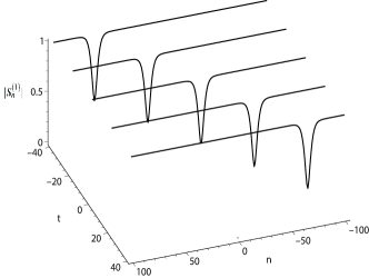
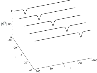
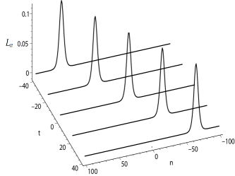
Figure 3: The profiles of evolutions of one-soliton solution (dark soliton for SW components).

Two-soliton solution: By taking $N=2$ in (78), we get the tau functions for the two-soliton solution:

$$f_{n}=1+E_{1}+E_{2}+\left|\frac{(p_{1}-p_{2})(p_{1}-\bar{p}_{2})}{(p_{1}p_{2}-1)(p_{1}\bar{p}_{2}-1)}\right|^{2}E_{1}E_{2},$$ (87)

$$g^{(1)}_{n}=1+A_{1}E_{1}+A_{2}E_{2}+\left|\frac{(p_{1}-p_{2})(p_{1}-\bar{p}_{2})}{(p_{1}p_{2}-1)(p_{1}\bar{p}_{2}-1)}\right|^{2}A_{1}A_{2}E_{1}E_{2},$$ (88)

$$g^{(2)}_{n}=1+B_{1}E_{1}+B_{2}E_{2}+\left|\frac{(p_{1}-p_{2})(p_{1}-\bar{p}_{2})}{(p_{1}p_{2}-1)(p_{1}\bar{p}_{2}-1)}\right|^{2}B_{1}B_{2}E_{1}E_{2},,$$ (89)

where

$$E_{j}={\rm i}\frac{p_{j}-\bar{p}_{j}}{p_{j}\bar{p}_{j}-1}(p_{j}\bar{p}_{j})\exp(\xi_{i}+\bar{\xi}_{j}),$$

$$A_{j}=\frac{(p_{j}-\alpha^{(1)})(\bar{p_{j}}-\alpha^{(1)})}{(1-\alpha^{(1)}p_{j})(1-\alpha^{(1)}\bar{p_{j}})},\ \ B_{j}=\frac{(p_{j}-\alpha^{(2)})(\bar{p_{j}}-\alpha^{(2)})}{(1-\alpha^{(2)}p_{j})(1-\alpha^{(2)}\bar{p_{j}})},$$

and $\xi_{j}=(p_{j}-\frac{1}{p_{j}})t+\xi_{j,0}$ and $p_{j}$ are complex constants satisfying

$${-}\sum^{2}_{\mu=1}{\rm i}\frac{c^{(\mu)}}{2}\left(\alpha^{(\mu)}{-}\bar{\alpha}^{(\mu)}\right)[\frac{1}{(1{-}\alpha^{(\mu)}p_{j})(1{-}\bar{\alpha}^{(\mu)}\bar{p}_{j})}{+}\frac{1}{(1{-}\alpha^{(\mu)}\bar{p}_{j})(1{-}\bar{\alpha}^{(\mu)}p_{j})}]=\frac{1}{p_{j}}{+}\frac{1}{\bar{p}_{j}},$$ (90)

for $j=1,2$. Figure 4 exhibits such a two-soliton interaction with the parameters as $(c^{(1)},c^{(2)})=(\frac{1}{9},-\frac{1}{8})$, $\alpha^{(1)}=\frac{\sqrt{2}}{2}+\frac{\sqrt{2}}{2}{\rm i}$, $\alpha^{(2)}=\frac{1}{2}-\frac{\sqrt{3}}{2}{\rm i}$, $p_{1}=1-0.6714{\rm i}$, $p_{2}=0.5-1.5356{\rm i}$ and $\xi^{\prime}_{1,0}=\xi^{\prime}_{2,0}=0$.

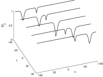
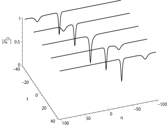
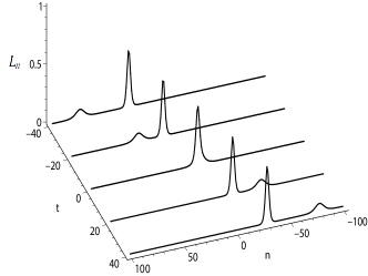
Figure 4: The profiles of evolutions of two-soliton solution (dark soliton for SW components).

5 Conclusion and discussions

In the present paper, we construct an integrable semi-discrete analogue of the coupled YO system by using Hirota’s bilinear method. Moreover, both the bright and dark soliton solutions in terms of pfaffians are derived based on the Bäcklund transformations of the semi-discrete BKP hierarchy. As far as we are aware of, it is the first time to propose an integrable semi-discrete YO system. There are several topics left for the study of the semi-discrete YO system, which are listed below:

1. The Lax pair, the bi-Hamiltonian structure and the conservation laws of this newly proposed semi-discrete YO system are not clear and deserve to be explored.

2. How to construct the inverse scattering transform scheme for the semi-discrete YO system is also an interesting problem.

3. It is of important to construct the mixed-type soliton solutions with both the bright and dark soliton for the vector semi-discrete YO system.

References

References

[1] Ablowitz M J and Clarkson P A 1991
Solitons, Nonlinear Evolution Equations and Inverse Scattering (London
Mathematical Society Lecure Notes Series) 149 (Cambridge:Cambridge Univ.
Press).
[2] Cheng Y 1992
J. Math. Phys.33 3774
[3] Loris I and Willox R 1997
Inverse Problems13 411
[4] Tsujimoto S 2000
in Applied Integrable Systems, ed. Y. Nakamura
(Shokabo, Tokyo) Chap. 1 [in Japanese]
[5] Narita K 1990
J. Phys. Soc. Jpn.59 3528
[6] Maruno K and Ohta Y 2006
J. Phys. Soc. Jpn.75 054002
[7] Doliwa A and Santini P M 1995
J. Math. Phys.36 1259
[8] Tsuchida T, Ujino H and Wadati M 1999
J. Phys. A: Math. Gen.32 2239
[9] Tsuchida T 2000
Rep. Math. Phys.46 269
[10]
Ohta Y 2009
Stud. Appl. Math.122 427
[11]
Feng B F, Ohta Y and Zhu Z 2015
submitted
[12] Willox R and Hattori M 2015
J. Math. Sci. Univ. Tokyo22 613
[13]
Levi D and Ragnisco O 2000
SIDE III: Symmetries and Integrability of Difference Equations
(CRM Proc. Lecture Notes vol 25) 25 (Providence, RI: American Mathematical
Society)
[14]
Zakharov V E 1972
Sov. Phys. JETP35 908
[15]
Yajima N and Oikawa M 1976
Prog. Theor. Phys.56 1719
[16]
Benny D J 1977
Stud. Appl. Math.56 15
[17]
Kivshar Y S 1992
Opt. Lett.17 1322
[18]
Chowdhury A and Tataronis J A 2008
Phys. Rev. Lett.100 153905
[19]
Davydov A S 1991
Solitons in molecular systems61 (Heidelberg: Springer)
[20]
Ma Y C and Redekopp L G 1979
Phys. Fluids22 1872
[21]
Ma Y C 1978
Stud. Appl. Math.59 201
[22]
Willox R 1999
Pseudo reductions of 2D Toda hierarchies in New
developments in soliton theory Proc. Riam, University of Kyushu, 10me-s1
75 [in japanese]
[23]
Chow W K, Chan N H, Kedziora D J and Grimshaw R H J 2013
J. Phys. Soc. Jpn.82 074001
[24]
Chen S, Grelu P and Soto-Crespo J M 2014
Phys. Rev. E89 011201
[25]
Zhang Y J and Cheng Y 1994
J. Math. Phys.35 5869
[26]
Sidorenko J and Strampp W 1993
J. Math. Phys.34 1429
[27]
Liu Q P 1996
J. Math. Phys.37 2307
[28]
Kanna T, Sakkaravarthi K and Tamilselvan K 2013
Phys. Rev. E88 062921
[29]
Sazonov S V and Ustinov N V 2011
JETP Lett.94 610
[30]
Myrzakulov R, Pashaev O K and Kholmurodov K T 1986
Phys. Scr.33 378
[31]
Khare A, Kanna T and Tamilselvan K 2014
Phys. Lett. A378 3093
[32]
Chen J, Chen Y, Feng B F and Maruno K 2015
J. Phys. Soc. Jpn.84 034002
[33]
Chen J, Chen Y, Feng B F and Maruno K 2015
J. Phys. Soc. Jpn.84 074001
[34]
Chen J, Chen Y, Feng B F and Maruno K 2015
Phys. Lett. A379 1510
[35]
Ablowitz M J and Ladik J F 1975
J. Math. Phys.16 598
[36]
Ablowitz M J and Ladik J F 1976
Stud. Appl. Math.55 213
[37]
Hirota R 1977
J. Phys. Soc. Jpn.43 1424
[38]
Hirota R 1977
J. Phys. Soc. Jpn.43 2074
[39]
Hirota R 1977
J. Phys. Soc. Jpn.43 2079
[40]
Date E, Jimbo M and Miwa T 1982
J. Phys. Soc. Jpn.51 4125
[41]
Date E, Jimbo M and Miwa T 1982
J. Phys. Soc. Jpn.51 4116
[42]
Date E, Jimbo M and Miwa T 1983
J. Phys. Soc. Jpn.52 388
[43]
Date E, Jimbo M and Miwa T 1983
J. Phys. Soc. Jpn.52 761
[44]
Date E, Jimbo M and Miwa T 1983
J. Phys. Soc. Jpn.52 766
[45]
Suris Y B 2003
The problem of integrable discretization: Hamiltonian approach219 (Springer Science)
[46]
Hu X B and Yu G F 2007
J. Phys. A: Math. Theor.40 12645
[47]
Hu X B, Li C X, Nimmo J J C and Yu G F 2005
J. Phys. A: Math. Gen.38 195 2005.
[48]
Ohta Y, Maruno K and Feng B F 2008
J. Phys. A: Math. Theor.41 355205
[49]
Feng B F, Maruno K and Ohta Y 2010
J. Comput. Appl. Math.235 229
[50]
Feng B F, Maruno K and Ohta Y 2010
J. Phys. A: Math. Theor.43 085203
[51]
Feng B F, Maruno K and Ohta Y 2015
J. Math. Phys.56 043502
[52]
Feng B F, Chen J, Chen Y, Maruno K and Ohta Y 2015
J. Phys. A: Math. Theor.48 385202
[53]
Feng B F, Maruno K and Ohta Y 2010
J. Phys. A: Math. Theor.43 265202
[54]
Feng B F, Maruno K and Ohta Y 2015
J. Phys. A: Math. Theor.48 135203
[55]
Vinet L and Yu G F 2013
J. Phys. A: Math. Theor.46 175205