Global results on reset-induced periodic trajectories of planar systems

Abstract

We study the existence of asymptotically stable periodic trajectories induced by reset feedback. The analysis is developed for a planar system. Casting the problem into the hybrid setting, we show that a periodic orbit arises from the balance between the energy dissipated during flows and the energy restored by resets, at jumps. The stability of the periodic orbit is studied with hybrid Lyapunov tools. The satisfaction of the so-called hybrid basic conditions ensures the robustness of the asymptotic stability. Extensions of the approach to more general mechanical systems are discussed.

I Introduction

Starting from the important theorem of Poincaré-Bendixson, many theoretical efforts have been made in the characterization of periodic orbits for planar continuous-time nonlinear systems, motivated by the pervasive presence of oscillators in electronics, mechanics and biology [5, 3]. A recent research direction seeks to extend this effort to the hybrid setting, namely to the context where, for a planar dynamical system, a suitable interplay of continuous flow and discrete jumps of the solutions leads to the existence of attractive periodic hybrid trajectories. The relevance of this topic in engineering is readily shown by the studies on bipedal robotic walking, where periodic hybrid trajectories arise from the combination of the free motion of the legs (continuous flow) with the impulsive action of the impacts at ground contact (discrete jumps) [14, 13].

The paper provides a stability analysis of hybrid periodic trajectories for planar mechanical systems based on the hybrid Lyapunov stability tools in [1]. The main motivation for the paper comes from the literature on variable impedance actuators, typically adopted in robotics. Strongly inspired by biological musculoskeletal systems, these actuators have a tunable stiffness and/or damping, which play a relevant role to improve motion efficiency [4, 9, 8, 7]. For multi-body systems with frequency separation between first and subsequent natural modes, [6] and [9] show that periodic oscillations can be obtained by means of simple switching control laws tuned only on the first natural mode. Taking advantage of a number of hybrid tools, we revisit and extend the results in [6]. We model the dynamics in [6] as a hybrid system and we show the existence of a unique (hybrid) periodic orbit arising when the energy dissipated during flow balances the energy restored by the reset-control action at a jump. The stability analysis exploits hybrid Lyapunov methods. In particular, the asymptotic stability of the periodic orbit follows from the decay along system trajectories of a suitable Lyapunov function tailored on the kinetic and potential energies just after and just before a jump.

The most relevant advantage of the approach is the intrinsic (in-the-small) robustness of asymptotic stability [1, Chapter 7], which makes possible the use of the reset feedback law in applications. The robustness of the design guarantees that the stability of the attractor persists, and is degraded with continuity, in the presence of small parameter perturbation or when the instantaneous reset law is replaced by a (sufficiently) fast continuous actuation.

The asymptotic stability of the attractor holds for any parameters configuration that allows for a unique periodic orbit. This follows from the fact that the Lyapunov function is based on the mechanical energy just after and just before a jump. Its minimum is represented on the phase space by the set of points such that the dissipated and restored mechanical energy are balanced. Its decay is a natural consequence of the mechanical features of the system. Indeed, no explicit characterization of the periodic orbit is required.

We anticipate that our Lyapunov-based analysis has similarities with the classical Poincaré analysis of periodic orbits. The level sets of the Lyapunov function are univocally identified by the points of the hyperplane at which resets occur. This hyperplane plays the role of a Poincaré section. Namely, along the portion of trajectory starting from and returning to this hyperplane, the overall decay of our Lyapunov function captures the convergence of the return map towards the fixed point. The advantage of a Lyapunov analysis is the characterization of the basin of attraction of the periodic orbit. In this sense, our approach is close in nature to the analysis of the rimless wheel in [12].

A promising future direction from our results is to exploit the hybrid framework to provide mixed continuous-discrete control strategies to optimize motion efficiency.

The paper is organized as follows. The hybrid dynamics is discussed in Section II. Sections III and IV provide conditions for the existence of periodic hybrid trajectories and for their stability. Technical proofs are in the Appendix. Simulations in Section V illustrate the convergence towards the unique hybrid periodic orbit of the system. A comparison with the literature and further discussions are reported in Section VI.

II System description

Based on [6], consider the classical mass-spring-damper mechanical system

$$m\ddot{q}+c\dot{q}+k(q-\theta)=0$$ (1)

with mass, damping and elastic constants respectively $m$, $c$, $k$. $q$ is the displacement of the mass and $\theta$ is the control input. The elastic force provided by the spring is proportional to the difference $q-\theta$. The role of $\theta$ is to enforce a variation in the stored potential energy of the spring. Following [4], $\theta$ could model the effect of the slow preloading of the spring during the flight phase of a hopping robot, which is then released by a clutch mechanism when touching the ground.

In what follows $\theta$ is piecewise constant: it switches between $\theta\in\{-\hat{\theta}/2,\hat{\theta}/2\}$ when the trajectories of the system pass through the hyperplane defined by $\{(q,\dot{q})\in{}^{2}\,|\,q-\theta=0\}$. $\hat{\theta}>0$ is a design parameter corresponding to the amount of potential energy loaded in the spring at switches. Switches on $\theta$ can be considered as the limit of a very fast continuous action on the spring, a kick of energy, rapidly moving $\theta$ from one value to the other in $\{-{\hat{\theta}}/{2},\hat{\theta}/2\}$.

With coordinates $x_{1}:=q-\theta$ and $x_{2}:=\dot{q}$, the dynamics of the system can be represented according to the hybrid formalism in [1] as follows. Since $\theta$ is constant, the flow dynamics reads

$$\dot{x}=f(x):=\begin{bmatrix}x_{2}\\ -\frac{c}{m}x_{2}-\frac{k}{m}x_{1}\end{bmatrix},\,x\in{\mathcal{C}}.$$ (2a)

The flow set $${\mathcal{C}}$$ enabling flow dynamics is given by

$${\mathcal{C}}=\{(x_{1},x_{2})\in{}^{2}\colon x_{1}x_{2}\leq 0\}\\ \cup\{(x_{1},x_{2})\in{}^{2}\colon|x_{1}|\geq\hat{\theta},x_{1}x_{2}\geq 0\}\ .$$ (2b)

The jump dynamics reads

$$x^{+}\in G(x):=\begin{bmatrix}\hat{\theta}\,\overline{\textrm{sgn}}(x_{2})\\ x_{2}\end{bmatrix},\,x\in{\mathcal{D}}$$ (2c)

where

$$\overline{\textrm{sgn}}(x_{2})=\begin{cases}\text{sign}(x_{2})&\ \text{ if }x_{2}\neq 0\vspace{1mm}\\ \{1,-1\}&\ \text{ if }x_{2}=0\ .\end{cases}$$

The jump set $${\mathcal{D}}$$ enabling jump dynamics is given by

$${\mathcal{D}}=\{(x_{1},x_{2})\in{}^{2}\colon x_{1}=0\}\ .$$ (2d)

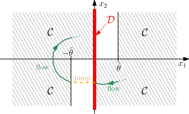
Figure 1: Flow set ${\mathcal{C}}$ and jump set ${\mathcal{D}}$ on the phase plane.

Figure 1 provides a graphical illustration of the flow and jump set on the system phase plane. (2d) guarantees that jumps occur when $q-\theta=x_{1}=0$. For $x_{2}\neq 0$, we have that $|x_{1}|$ is reset from $0$ to $|x_{1}^{+}|=\hat{\theta}$ that is, $|q^{+}-{\theta}^{+}|=|q-{\theta}^{+}|=\hat{\theta}$. Indeed, the reset corresponds to a switch in the equilibrium position of the spring, through actuation. We do not reset the mass position $q$.

The behavior of the solutions is illustrated in Figure 2, which for a system with parameters $m=1$ kg, $c=0.3$ Ns/m, $k=1$ N/m, $\hat{\theta}=0.2$ m, for two different initial conditions. The two trajectories converge asymptotically to an attractor defined by the image of a hybrid periodic trajectory, where periodicity must be intended in a hybrid sense as clarified in the next section.

Remark 1

In (2c) we used the set-valued mapping $\overline{\textrm{sgn}}$ to guarantee that the graph of the jump map $x\mapsto G(x)$ is a closed set. This feature ensures the outer semicontinuity of $G$. Outer semicontinuity of $G$ combined with the continuity of $f$ and with the fact that ${\mathcal{C}}$ and ${\mathcal{D}}$ are closed sets guarantees that hybrid system (2) satisfies the hybrid basic conditions [1, Assumption 6.5]. They guarantee regularity of the solution set and robustness to small perturbations [2].   $\lrcorner$

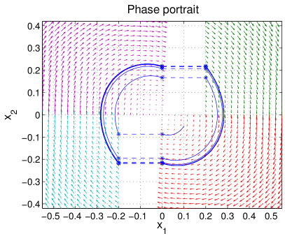
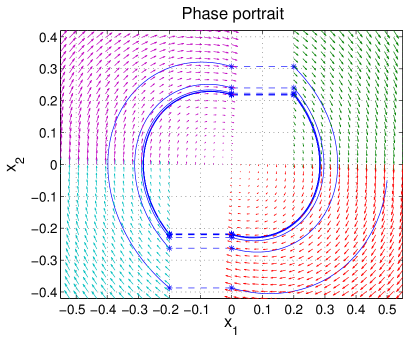
Figure 2: Phase plot of hybrid trajectories. Left: $(x_{1,0},x_{2,0}):=(0.1,-0.05)$. Right: $(x_{1,0},x_{2,0}):=(0.5,-0.05)$.

III Hybrid periodic orbits

The notion of periodicity for a hybrid trajectory is a straightforward extension of the usual notion of periodicity.

Definition 1

Given any hybrid system $\mathcal{H}:=({\mathcal{C}},F,{\mathcal{D}},G)$, a hybrid periodic trajectory is a complete solution $x$ for which there exists a pair $(T,J)$ with either $T\in{}_{\geq 0}$ and $J\in\mathbb{Z}_{>0}$ or $T\in{}_{>0}$ and $J\in\mathbb{Z}_{\geq 0}$ such that $(t,j)\in\text{dom}(x)$ implies $(t+T,j+J)\in\text{dom}(x)$ and, moreover,

$$x(t,j)=x(t+T,j+J).$$ (3)

The image of $x$ is a hybrid periodic orbit.

The following standing assumption on the parameters of the hybrid dynamics (2) is necessary for the existence of a nontrivial hybrid periodic trajectory.

Assumption 1

$\hat{\theta}$, $m$, $c$ and $k$ are strictly positive. The roots of $ms^{2}+cs+k=0$ are complex conjugate, that is $\left(\frac{c}{2m}\right)^{2}-\frac{k}{m}<0$.

Assumption 1 guarantees that $m\ddot{x}_{1}+c\dot{x}_{1}+kx_{1}=0$ is an underdamped mechanical system [10, Chap. 2.2]. When the system is not underdamped there is no guarantee that a nontrivial hybrid periodic trajectory exists. With real eigenvalues in the flow map, the trajectories of the system may converge to the origin according to the direction of the eigenvector corresponding to the slowest eigenvalue, lying in the second/fourth quadrant for $m,c,k>0$. In such a case, the solutions to (2) exhibit at most one jump and the origin is a globally asymptotically stable equilibrium.

The existence of a nontrivial hybrid periodic orbit follows from energy considerations. Consider the -shaped curve ${\mathcal{C}}_{0}$ represented in Figure 3, given by the set

$${\mathcal{C}}_{0}=\{x\in{}^{2}\colon|x_{1}|=\hat{\theta},x_{1}x_{2}\geq 0\}\\ \cup\{x\in{}^{2}\colon|x_{1}|\leq\hat{\theta},x_{2}=0\}.$$ (4)

Under Assumption 1, the trajectories starting from ${\mathcal{C}}_{0}$ necessarily flow until they reach ${\mathcal{D}}$. More specifically, flowing solutions from any $x\in{\mathcal{C}}$ in forward (respectively, backward) time reach set ${\mathcal{D}}$ (respectively, ${\mathcal{C}}_{0}$) in finite time because of the revolving nature of the flow trajectories. The following quantities are thus well defined.

• Backward energies. Denoting by $(x_{1b},x_{2b})$ the intersection with ${\mathcal{C}}_{0}$ after flowing in backward time from $x$,

  $$T_{b}(x):=\frac{1}{2}mx_{2b}^{2}\quad\qquad U_{b}(x):=\frac{1}{2}kx_{1b}^{2}$$ (5a)

  are the backward kinetic and backward potential energies, respectively.

• Forward energies. Denoting by $(x_{1f},x_{2f})$ the intersection with ${\mathcal{D}}$ after flowing in forward time from $x$,

  $$T_{f}(x):=\frac{1}{2}mx_{2f}^{2}$$ (5b)

  is the forward kinetic energy.

Figure 3 shows the level sets of $T_{b}$, $U_{b}$ and $T_{f}$, which correspond indeed to flowing portions of solutions to (2).

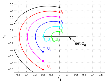
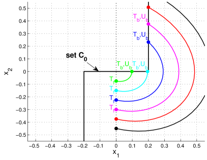
Figure 3: Set ${\mathcal{C}}_{0}$. Flowing solutions. The curves from ${\mathcal{C}}_{0}$ to ${\mathcal{D}}$ are level sets of $T_{b}$, $U_{b}$ and $T_{f}$.

For each $x\neq 0$ the quantity $T_{b}(x)+U_{b}(x)$ is the total mechanical energy of the system right after a jump. The quantity $T_{f}(x)$ is the total mechanical energy of the system after a maximal flow, that is, right before a jump. The difference between these two energies corresponds to the dissipation during flows.

The reset of $\theta$ injects energy into the system in the form of potential energy. This fact and the central symmetry of the phase portrait (namely, if $\phi$ is a solution to (2), $-\phi$ is a solution as well) imply that a hybrid periodic orbit corresponds to the set of points satisfying the energy balance

$$T_{b}(x)+U_{b}(x)=T_{f}(x)+\frac{1}{2}k\hat{\theta}^{2}\,$$ (6)

where the last term represents precisely the potential energy injected by a reset. Given the mentioned central symmetry, $x\neq 0$ belongs to a periodic hybrid orbit only if $U_{b}(x)=\frac{1}{2}k\hat{\theta}^{2}$, so that (6) is equivalent to $T_{b}(x)=T_{f}(x)$.

Existence and uniqueness of the hybrid periodic orbit follows from the monotonicity of the dissipation with respect to initial conditions on ${\mathcal{C}}_{0}$. In fact, for $x=(x_{1},x_{2})\in{\mathcal{C}}_{0}$ the dissipation is a strictly increasing function of $|x|$. This is precisely stated in the next lemma, proven in the Appendix.

Lemma 1

Consider any solution $x$ to (2) flowing from ${\mathcal{C}}_{0}$ at ordinary time $t_{1}$ to ${\mathcal{D}}$ at ordinary time $t_{2}\geq t_{1}$ and define the total mechanical energy at $x$ as $E(x)=\frac{1}{2}mx_{2}^{2}+\frac{1}{2}kx_{1}^{2}$. The dissipated energy $E(x(t_{1}))-E(x(t_{2}))$ is equal to $c\Pi$, where $\Pi$ is the (unsigned) area within the curves given by the image of the solution, the set ${\mathcal{C}}_{0}$ and the set ${\mathcal{D}}$ (hatched area in Figure 4).

The monotonicity of the dissipation is clear from Figure 4. As a consequence, there is only one initial condition on ${\mathcal{C}}_{0}$ for which (6) holds.

Theorem 1

Under Assumption 1, there exists a unique nontrivial hybrid periodic orbit for the hybrid system (2). $T_{b}(x)=T_{f}(x)$ at each point $x$ of the hybrid periodic orbit.

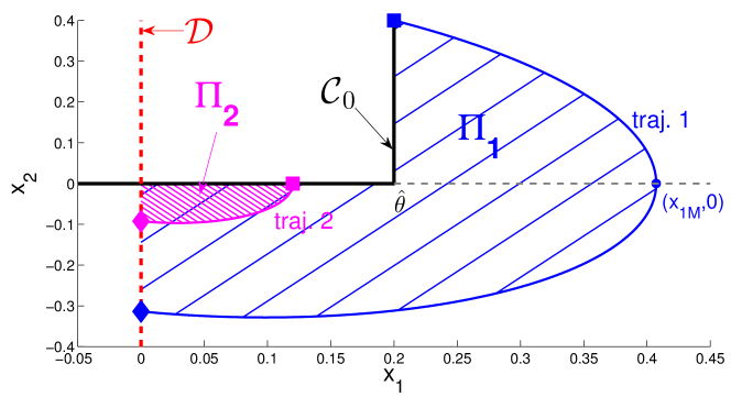
Figure 4: The hatched areas is proportional to the energy dissipated by damping.

IV Global asymptotic stability

The stability of the nontrivial hybrid periodic orbit is a set stability problem. Consider the attractor given by

$$\mathcal{A}=\{x\in{\mathcal{C}}\colon T_{b}(x)=T_{f}(x),x\neq 0\}\ .$$ (7)

Energy considerations similar to those in the previous section readily show that $\mathcal{A}$ is compact and forward invariant (see the proof of Lemma 2). The images of all nontrivial hybrid periodic trajectories of (2) coincide with $\mathcal{A}$. Convergence and stability of the periodic motion follow from the next theorem.

Theorem 2

Under Assumption 1, the set $\mathcal{A}$ in (7) is an asymptotically stable attractor for the hybrid system (2) with basin of attraction $\mathcal{B}_{\mathcal{A}}={}^{2}\backslash\{0\}$.

The origin $x=0$ is not in $\mathcal{B}_{\mathcal{A}}$ because it is a weak equilibrium: solutions to (2) starting from the origin can flow forever staying at the origin or may jump to $-\hat{\theta}$ or $\hat{\theta}$ and then converge to the hybrid periodic orbit.

We remark that the stability of the set $\mathcal{A}$ does not require an explicit characterization of the hybrid periodic orbit. We only need to ensure the feasibility of the balance in (6). Therefore, by Theorem 1 and Theorem 2, the reset feedback law induces a hybrid periodic trajectory for every parameters selection that satisfies Assumption 1. Then future work comprises performing optimal selections of $\theta$ (and the arising periodic motion) via hybrid adaptation.

The proof of Theorem 2 is based on a Lyapunov argument. Using the definitions in (5), consider the Lyapunov function candidate for $\mathcal{A}$ given by

$$V(x)=\frac{(U_{b}(x)+T_{b}(x)-T_{f}(x)-\frac{1}{2}k\hat{\theta}^{2})^{2}}{U_{b}(x)}\ .$$ (8)

The shape and the level sets of $V$ are illustrated in Figure 5. Note that the Lyapunov function $V$ blows up as $x$ approaches $0$ (the boundary of $\mathcal{B}_{\mathcal{A}}$) and as $x$ grows unbounded, as shown in Figure 5 for the same parameter selection of Figure 2.

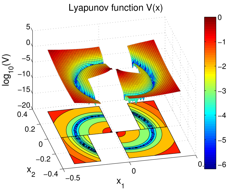
Figure 5: The Lyapunov function $V$ in logarithmic scale.

The next lemma is a key step for proving Theorem 2.

Lemma 2

Under Assumption 1, the set $\mathcal{A}$ in (7) is nonempty and compact and the Lyapunov function $V$ in (8)

1. is positive definite with respect to $\mathcal{A}$ on $\mathcal{B}_{\mathcal{A}}\cap({\mathcal{C}}\cup{\mathcal{D}})$, namely

   $$V(x) =0\text{ if }x\in\mathcal{A}$$ (9a)

   $$V(x) >0\text{ if }x\in\mathcal{B}_{\mathcal{A}}\cap({\mathcal{C}}\cup{\mathcal{D}})\backslash\mathcal{A}$$

   $$\lim_{\begin{subarray}{c}|x|\rightarrow 0^{+}\\ |x|\rightarrow+\infty\end{subarray}}V(x) =+\infty$$

2. is constant in the flow direction

   $$\left<\nabla V(x),f(x)\right>=0,\,\,\forall x\in{\mathcal{C}}$$ (9b)

3. provides strict decrease across jumps

   $$V\left(G(x)\right)-V(x)<0,\,\,\forall x\in\mathcal{B}_{\mathcal{A}}\cap{\mathcal{D}}\backslash\mathcal{A}.$$ (9c)

Remark 2

Following [1, Corollary 7.32] and [1, Definition 7.29]), item (i) of Lemma 2 implies that for any indicator function $\omega$ of $\mathcal{A}$ on $\mathcal{B}_{\mathcal{A}}$ there exists class $\mathcal{K}_{\infty}$ functions $\underline{\alpha}$ and $\overline{\alpha}$ such that

$$\underline{\alpha}(\omega(x))\leq V(x)\leq\overline{\alpha}(\omega(x)),$$ (10)

which entails standard additional features of $\mathcal{A}$, e.g., robustness and semiglobal-practical robustness of asymptotic stability of $\mathcal{A}$ [1, Chap. 6.7].   $\lrcorner$

Based on Lemma 2, the proof of Theorem 2 is a mere application of fundamental Lyapunov results holding for hybrid systems described with the formalism in [1]. In particular, Lemma 2 establishes that function $V$ in (8) is a non-strict Lyapunov function for compact attractor ${\mathcal{A}}$, in the sense of [11, Equations (6a), (7)]. Indeed, the fact that ${\mathcal{A}}$ is compact is sufficient to obtain that (9a) implies (10) for any indicator function $\omega$ and suitable class ${\mathcal{K}}_{\infty}$ functions $\underline{\alpha}$, $\overline{\alpha}$. Moreover, (9b) coincides with [11, Equation (7a)] and (9c) implies [11, Equation (7b)] for a suitable positive definite function $\rho$, once again because ${\mathcal{A}}$ is compact. As a consequence, we may apply a local generalization of [11, Theorem 2] by noticing that all solutions to (2) are semiglobally persistently jumping, namely for any arbitrarily large number $\Delta$, we have that solutions restricted to flow in ${\cal C}\cap{\Delta{\mathbb{B}}}\cap{\mathcal{B}}_{\mathcal{A}}$ and jump from ${\cal D}\cap{\Delta{\mathbb{B}}}\cap{\mathcal{B}}_{\mathcal{A}}$ have a uniform reverse dwell time (i.e., a maximum time between each pair of consecutive jumps in their domain). Such a maximum time is easily computed as the minimum flow time from the vertical portion of ${\mathcal{C}}_{0}$ intersected with $\Delta{\mathbb{B}}$. Note, in particular, that by homogeneity of the linear flow equation, such a maximum flow time is strictly smaller than the flow time of the first flowing interval of the (unique) solution starting from $x(0)=\left[\begin{smallmatrix}\hat{\theta}\\ \Delta\end{smallmatrix}\right]$.

V Simulations

We simulate the hybrid system (2) with the same parameters adopted in Figure 2, corresponding to $m=1$ kg, $c=0.3$ Ns/m, $k=1$ N/m (eigenvalues $s_{1,2}=-0.15\pm i0.9887$, consistent with Assumption 1). Instead of $\hat{\theta}=0.2$ m we enforce a reset to the larger value $\hat{\theta}=0.3$. Compared to Figure 2, the hybrid periodic orbit changes as shown in the upper part of Figure 6. The bottom part of Figure 6 shows the values of the Lyapunov function and of the states $(x_{1},x_{2})$ as functions of ordinary time.

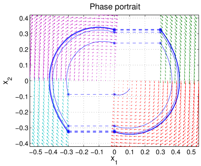
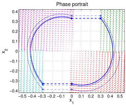
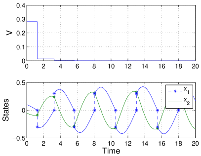
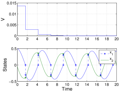
Figure 6: Upper part: phase plot of the trajectories. Bottom part: Lyapunov function and hybrid trajectories projected on ordinary time for the two initial conditions. Left: initial condition $(0.1,-0.05)$. Right: initial condition $(0.5,-0.05)$.

VI Conclusions and future research

Following [6], different hybrid periodic orbits can be generated by exploiting different reset laws. Within the hybrid characterization (2), one of the switching laws proposed in [6] is captured by the flow and jump sets ${\mathcal{C}}$ and ${\mathcal{D}}$ given in Figure LABEL:fig:CandDdlrII: $\hat{\theta}\geq 2\epsilon_{\phi}$ and $\epsilon_{\phi}>0$ is a new control parameter. $G(x)=\!\left[\begin{smallmatrix}x_{1}+\hat{\theta}\mathrm{sign}(x_{2})\\ x_{2}\end{smallmatrix}\right]$ and $f(x)$ remains (2a) with the parameters of Section V. The simulation of a number of trajectories is reported in Figure LABEL:fig:trajdlrII. The approach and results in Sections III and IV can be extended to capture the stability properties of this new hybrid system, to show the existence of a globally asymptotically stable hybrid periodic orbit.

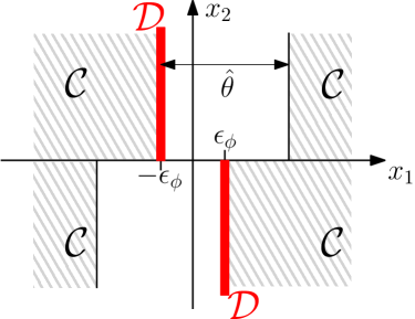
(a)

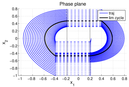
(b)

Figure 7: $\epsilon_{\phi}=0.2$ and $\hat{\theta}=0.6$.

Figure 7 shows the potential of the hybrid characterization in (2). A number of reset feedback laws can be modeled by variations on the definitions of the sets ${\mathcal{C}}$ and ${\mathcal{D}}$ and of the jump map $G$. The monotonicity of the dissipated energy is crucial for the uniqueness of the attractor. Future research will investigate the family of reset feedback that guarantees existence and uniqueness of an asymptotically stable hybrid periodic orbit.

It is natural to consider mechanical systems with elastic potentials typical of nonlinear springs, so that (2a) would read $\dot{x}_{2}=-\frac{c}{m}x_{2}-\frac{1}{m}\frac{\partial U}{\partial x_{1}}$ where the potential $U$ is any positive definite function. A necessary condition for the existence of an attractor with basin ${}^{2}\backslash\{0\}$ is the strict monotonicity of the elastic potential, namely the positivity of the function $x_{1}\mapsto x_{1}\frac{\partial U(x_{1})}{\partial x_{1}}$. In fact, the lack of strict monotonicity may lead to the coexistence of several attractors. The minimal requirement for the existence of globally attractive hybrid periodic orbits is that the linearization of the flow dynamics at the origin has complex conjugate eigenvalues, which is a straightforward generalization of Assumption 1. Otherwise, trajectories that are sufficiently close to the origin would flow towards it remaining in the second/fourth quadrant, without triggering any reset. Future work will look for tight sufficient conditions for the existence of a global attractor for general elastic potentials.

Finally, the generality of a Lyapunov approach for stability analysis calls for extensions of the method to more general mechanical systems. The first step is the analysis of $n$-dimensional linear mechanical systems perturbed by resets. We also recall that the model in (2), albeit an abstraction, stems from the robotics context. Further detailed analysis will investigate its potential for robotic applications, in particular the one of legged locomotion.

-A Proof of Lemma 1

The work performed by the nonconservative viscous force $F_{d}=cx_{2}$ in moving the point mass from position 1 to position 2 causes a change $E_{2}-E_{1}$ in the total mechanical energy [10, Page 9]. With the aid of Figure 4, let us exemplify it on trajectories like 1 and denote $x_{1M}$ the value at which a trajectory crosses the line $x_{2}=0$, so that on the trajectory $x_{2}$ can be expressed as function of $x_{1}$ for each half-plane $x_{2}>0$, $x_{2}<0$. Then, by splitting the integral relative to the work in two pieces, we get $E(x(t_{2}))-E(x(t_{1}))=\int^{x_{1M}}_{\hat{\theta}}\!\!-(cx_{2})dx_{1}+\int_{x_{1M}}^{0}\!\!\!-(cx_{2})dx_{1}=-c\Pi$.

-B Proof of Lemma 2

The proof of this fact relies on Lemma 1. From (8),

$$V(x) =\frac{\Big{(}\overbrace{U_{b}(x)+T_{b}(x)}^{E_{b}(x)}-\overbrace{T_{f}(x)}^{E_{f}(x)}-\overbrace{\frac{1}{2}k\hat{\theta}^{2}}^{\hat{U}}\Big{)}^{2}}{U_{b}(x)}$$

$$=\frac{(c\Pi(x)-\hat{U})^{2}}{U_{b}(x)},$$ (11)

where $E_{b}$ and $E_{f}$ are the total energies of the system right after and right before a jump, respectively; $\hat{U}$ is the potential energy at $\left[\begin{smallmatrix}\hat{\theta}\\ 0\end{smallmatrix}\right]\in{\mathcal{C}}_{0}$; $\Pi(x)$ is the area spanned by the solution passing through $x$ during a flow from ${\mathcal{C}}_{0}$ to ${\mathcal{D}}$ (where $E_{f}$ is evaluated); and $c>0$ is the damping coefficient in (1). Figure 4 provides two examples for $\Pi(x)$.

We are now ready to prove Lemma 2. First notice that, due to the uniqueness of flowing solutions, the function $x\mapsto\Pi(x)$ is necessarily strictly increasing as $x$ moves farther from the origin (or any compact set). Denote by $c\Pi_{0}=c\Pi\left(\left[\begin{smallmatrix}\hat{\theta}\\ 0\end{smallmatrix}\right]\right)$ the dissipated energy when starting from the corner of set ${\mathcal{C}}_{0}$ in (4). Moreover, denote by $c{\Pi^{\star}}=\frac{1}{2}k\hat{\theta}^{2}=\hat{U}$ the dissipated energy associated to the hybrid periodic orbit. Note that ${\Pi^{\star}}>\Pi_{0}$ necessarily, because $c\Pi_{0}$ cannot be larger than the total energy $\hat{U}=c{\Pi^{\star}}$ at the beginning of the corresponding solution starting from the corner of ${\mathcal{C}}_{0}$. Then,

$$\mathcal{A}=\{x\in{\mathcal{C}}\colon\Pi(x)={\Pi^{\star}},\,x\neq 0\},$$ (12)

which proves that it is non-empty and compact. We prove now the three items of the Lemma.

Item (i). Since $V(x)$ in (11) is non-negative and zero if and only if $\Pi(x)={\Pi^{\star}}$, from expression (12) we obtain $V(x)=0$ if and only if $x\in\mathcal{A}$ and positive otherwise. Moreover, as $x$ approaches zero, we have that $U_{b}(x)$ tends to zero, which implies $V(x)\to\infty$. Since $U_{b}(x)\leq\hat{U}$ for all $x$ due to the structure of ${\mathcal{C}}_{0}$, $\lim_{|x|\to\infty}\Pi(x)=+\infty$ implies $\lim_{|x|\to\infty}V(x)=+\infty$.

Item (3). This item follows in a straightforward way from the fact that $V(x)$ remains constant by construction during flow.

Item (4). First of all notice that $x=\!\left[\begin{smallmatrix}x_{1}\\ x_{2}\end{smallmatrix}\right]\!\in{\mathcal{D}}$ implies $x_{1}=0$ and that $G(x)=\left[\begin{smallmatrix}\hat{\theta}\text{sign}(x_{2})\\ x_{2}\end{smallmatrix}\right]$ for all $x\in{\mathcal{D}}\cap\mathcal{B}_{\mathcal{A}}$. We split the proof in three cases. We only consider jumps from points in the negative part of ${\mathcal{D}}$ (namely $x_{2}<0$) because of the central symmetry of the phase portrait. We also use the simplified notation $\Pi^{+}$ to denote $\Pi(x^{+})$. Similar simplifications will be used for other quantities.

Case 1: $\Pi>{\Pi^{\star}}>\Pi_{0}$. First of all, by uniqueness of solutions $\Pi^{+}>{\Pi^{\star}}$, otherwise the flow would intersect the hybrid periodic orbit. Consider the left part of Figure 8 and note that $\Pi>{\Pi^{\star}}$ implies $\Pi^{+}<\Pi$. Indeed, exploiting $U_{b}^{+}=U_{b}=\hat{U}=c\Pi^{\star}$ and $T_{b}+U_{b}=T_{f}+c\Pi$ and $T_{b}^{+}=T_{f}$, we get $T_{b}=T_{f}+c\Pi-c\Pi^{\star}>T_{f}=T_{b}^{+}$. $\Pi>\Pi^{+}$ follows by monotonicity. Finally, the result is proven from

$$0=c{\Pi^{\star}}-\hat{U}<c\Pi^{+}-\hat{U}<c\Pi-\hat{U}.$$

Case 2: ${\Pi^{\star}}>\Pi>\Pi_{0}$. First of all, $\Pi^{+}<{\Pi^{\star}}$ again from uniqueness of solutions. Consider the right-part of Figure 8 and note that $\Pi_{0}<\Pi<{\Pi^{\star}}$ implies $\Pi^{+}>\Pi$. In fact, following the argument of Case 1, we have that $U_{b}^{+}=U_{b}=\hat{U}=c\Pi^{\star}$ and $T_{b}+U_{b}=T_{f}+c\Pi$ and $T_{b}^{+}=T_{f}$ thus $T_{b}=T_{f}+c\Pi-c\Pi^{\star}<T_{f}=T_{b}^{+}$. The result is proven from

$$0=c{\Pi^{\star}}-\hat{U}>c\Pi^{+}-\hat{U}>c\Pi-\hat{U}.$$

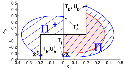
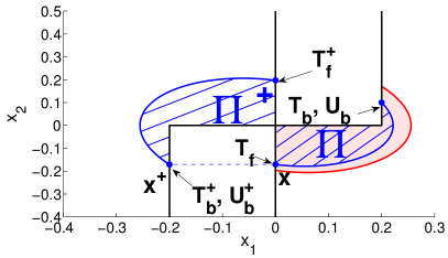
Figure 8: Left: $\Pi>{\Pi^{\star}}>\Pi_{0}$. Right: ${\Pi^{\star}}>\Pi>\Pi_{0}$. Pink areas are $\Pi^{+}$ mirrored about the origin.

Case 3: $0<\Pi<\Pi_{0}$. Consider Figure 9. In this case we have $U_{b}<\hat{U}$ because $U_{b}$ is evaluated on the horizontal part of ${\mathcal{C}}_{0}$. Then

$$V^{+}-V ={(c\Pi^{+}-\hat{U})^{2}}\big{/}{\hat{U}}-{(c\Pi-\hat{U})^{2}}\big{/}{U_{b}}$$

$$<{(c\Pi^{+}-\hat{U})^{2}}\big{/}{\hat{U}}-{(c\Pi-\hat{U})^{2}}\big{/}{\hat{U}}.$$

Now, observe that $c\Pi^{+}<\hat{U}=c\Pi^{\star}$ because otherwise the forward solution from $x^{+}$ would intersect the flowing portion of the hybrid periodic orbit (thus contradicting uniqueness). Then, using $U_{b}>0$, we get $V^{+}-V<0$ from

$$(c\Pi^{+}-\hat{U})^{2}-(c\Pi-\hat{U})^{2}$$

$$\qquad=c(\underbrace{\Pi^{+}-\Pi}_{>0})(\underbrace{c\Pi^{+}-\hat{U}}_{<0}+\underbrace{c\Pi-\hat{U}}_{<0})<0,$$

where we used (i) $\Pi^{+}>\Pi$ from $\Pi^{+}$ being evaluated from the vertical part of ${\mathcal{C}}_{0}$ and (ii) $c\Pi<\hat{U}$ from $c\Pi<U_{b}$.

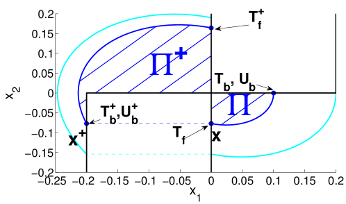
Figure 9: Case 3: $0<\Pi<\Pi_{0}$.

References

- [1] R. Goebel, R. G. Sanfelice, and A. R. Teel, Hybrid Dynamical Systems: modeling, stability, and robustness. Princeton University Press, 2012.
- [2] R. Goebel and A. R. Teel, “Solutions to hybrid inclusions via set and graphical convergence with stability theory applications,” Automatica, vol. 42, no. 4, pp. 573–587, 2006.
- [3] J. Grasman, Asymptotic methods for relaxation oscillations and applications, 1st ed., ser. Applied Mathematical Sciences. Springer, 1987.
- [4] F. Gunther and F. Iida, “Preloaded hopping with linear multi-modal actuation,” in IEEE/RSJ International Conference on Intelligent Robots and Systems, 2013, pp. 5847–5852.
- [5] M. Hirsch and S. Smale, Differential Equations, Dynamical Systems, and Linear Algebra (Pure and Applied Mathematics, Vol. 60). Academic Press, 1974.
- [6] D. Lakatos and A. Albu-Schäffer, “Switching based limit cycle control for compliantly actuated second-order systems,” in Proceedings of the 19th IFAC World Congress, 2014, pp. 6392–6399.
- [7] D. Lakatos, G. Garofalo, A. Dietrich, and A. Albu-Schäffer, “Jumping control for compliantly actuated multilegged robots,” in IEEE International Conference on Robotics and Automation, 2014, pp. 4562–4568.
- [8] D. Lakatos, G. Garofalo, F. Petit, C. Ott, and A. Albu-Schäffer, “Modal limit cycle control for variable stiffness actuated robots,” in IEEE International Conference on Robotics and Automation, 2013, pp. 4934–4941.
- [9] D. Lakatos, F. Petit, and A. Albu-Schäffer, “Nonlinear oscillations for cyclic movements in variable impedance actuated robotic arms,” in IEEE International Conference on Robotics and Automation, 2013, pp. 508–515.
- [10] L. Meirovitch, Fundamentals of Vibrations. McGraw-Hill Companies, 2000.
- [11] C. Prieur, A. Teel, and L. Zaccarian, “Relaxed persistent flow/jump conditions for uniform global asymptotic stability,” IEEE Transactions on Automatic Control, vol. 59, no. 10, pp. 2766–2771, 2014.
- [12] C. O. Saglam, A. R. Teel, and K. Byl, “Lyapunov-based versus Poincaré map analysis of the rimless wheel.” in IEEE 53rd Conference on Decision and Control, 2014, pp. 1514–1520.
- [13] A. R. Teel, R. Goebel, B. Morris, A. D. Ames, and J. W. Grizzle, “A stabilization result with application to bipedal locomotion,” in IEEE 52nd Conference on Decision and Control, 2013, pp. 2030–2035.
- [14] E. Westervelt, J. Grizzle, C. Chevallereau, J. Choi, and B. Morris, Feedback control of dynamic bipedal robot locomotion, ser. Control and automation. Boca Raton: CRC Press, 2007.