Multiscale stabilization for convection-dominated diffusion in heterogeneous media

Abstract

We develop a Petrov-Galerkin stabilization method for multiscale convection-diffusion transport systems. Existing stabilization techniques add a limited number of degrees of freedom in the form of bubble functions or a modified diffusion, which may not sufficient to stabilize multiscale systems. We seek a local reduced-order model for this kind of multiscale transport problems and thus, develop a systematic approach for finding reduced-order approximations of the solution. We start from a Petrov-Galerkin framework using optimal weighting functions. We introduce an auxiliary variable to a mixed formulation of the problem. The auxiliary variable stands for the optimal weighting function. The problem reduces to finding a test space (a reduced dimensional space for this auxiliary variable), which guarantees that the error in the primal variable (representing the solution) is close to the projection error of the full solution on the reduced dimensional space that approximates the solution. To find the test space, we reformulate some recent mixed Generalized Multiscale Finite Element Methods. We introduce snapshots and local spectral problems that appropriately define local weight and trial spaces. In particular, we use energy minimizing snapshots and local spectral decompositions in the natural norm associated with the auxiliary variable. The resulting spectral decomposition adaptively identifies and builds the optimal multiscale space to stabilize the system. We discuss the stability and its relation to the approximation property of the test space. We design online basis functions, which accelerate convergence in the test space, and consequently, improve stability. We present several numerical examples and show that one needs a few test functions to achieve an error similar to the projection error in the primal variable irrespective of the Peclet number.

1 Introduction

Existing techniques for solving multiscale problems usually seek a reduced dimensional approximation for the solution space. Many of these multiscale problems with high contrast require stabilization due to the large variations in the medium properties. For example, in a multiscale convection-dominated diffusion with a high Peclet number, besides finding a reduced order model, one needs to stabilize the system to avoid large errors [56]. Stabilization of multiscale methods for convection-diffusion cannot simply use a modified diffusion and requires more sophisticated techniques. In this paper, we discuss a general framework for stabilization, which combines recent developments in Generalized Multiscale Finite Element Method (e.g., [33]) and Discontinuous Petrov-Galerkin method (e.g., [29, 54, 55]).

We consider a convection-diffusion equation in the form

$$-\nabla\cdot(\kappa\nabla u)+b\cdot\nabla u=f$$ (1)

with a high Peclet number, where $\kappa$ is a diffusion tensor and $b$ is the velocity vector [56, 41]. Both fields are characterized by multiscale spatial features. Many solution techniques for multiscale problems require a construction of special basis functions on a coarse grid [30, 57, 3, 37, 33, 38, 43, 42, 32, 34, 39, 16, 31, 12, 13, 46, 35]. These approaches include the Multiscale Finite Element Methods (MsFEM) [37, 33, 38, 39, 45, 2] and Variational Multiscale Methods [50, 48, 47, 6, 53, 9, 49, 23, 5, 1, 52] among others. In MsFEM, local multiscale basis functions are constructed for each coarse region. Recently, a general framework, the Generalized Multiscale Finite Element Method (GMsFEM), for finding a reduced approximation was proposed [33, 44, 45, 35, 36, 10, 21, 17, 11, 22, 19, 20]. GMsFEM generates a reduced dimensional space on a coarse grid that approximates the solution space by introducing local snapshot spaces and appropriate local spectral decompositions. However, a direct application of these approaches for singularly-perturbed problems, such as convection-dominated diffusion, faces difficulties due to the poor stability of these schemes. Simplified stabilization techniques on a coarse grid are not efficient. Indeed, the modification of the diffusion coefficient and similar approaches assumes the use of a few degrees of freedom locally to stabilize the problem. These approaches do not suffice for complex problems and one needs a systematic method to generate the necessary test spaces.

We use the discontinuous Petrov-Galerkin (DPG) techniques following [25, 15, 27, 29, 26, 58] to stabilize the system. We start with a stable fine-scale finite element discretization that fully resolves all scales of the underlying equation

$$Au=f.$$ (2)

The system is written in a mixed framework using an auxiliary variable as follows

$$Rw+Au =f,$$ (3)

$$A^{T}w\ \ \qquad =0.$$ (4)

The variable $w$ plays the role of a test function and the matrix $R$ is related to the norm in which we seek to achieve stability. We assume that the fine-scale system gives $w=0$, that is, it is discretely stable. In multiscale methods, one approximates the solution using a reduced dimensional subspace for $u$. More precisely,

$$u\approx\sum_{i}z^{u}_{i}\phi_{i},\qquad\text{ or }\qquad u\approx\Phi z^{u}.$$

The resulting system also needs a reduced dimensional test space,

$$w\approx\sum_{i}z^{w}_{i}\psi_{i}\qquad\text{ or }\qquad w\approx\Psi z^{w}.$$

The stabilization of (2) requires appropriate $\Phi$ and $\Psi$. We discuss the design of these spaces in the following.

Within the DPG framework, one can achieve stability by choosing test functions $w$ with global support [4, 28]. However, our goal is to design procedures for constructing localized test spaces. In this paper, we design a novel test space which guarantees stability for singularly perturbed problems such as convection-dominated diffusion in a multiscale media with a high Peclet number. To generate a multiscale space for $w$, we use the recently developed theory for GMsFEM for mixed problems [18]. We start by constructing a local snapshot space which approximates the global test functions. These snapshot vectors are supported in coarse regions and are constructed solving local adjoint problems in neighboring coarse elements. The snapshot spaces are augmented with local bubble functions. The dimension of the snapshot space is proportional to the number of fine-grid edges (i.e., proportional to the Peclet number). To reduce the dimension of this space, making the construction independent of the Peclet number, we propose a set of local spectral problems. In these local spectral problems, we use minimum energy snapshot vectors [14] and perform a local spectral decomposition with respect to the $AA^{T}$ norm. Our objective is to find a reduced dimensional approximation, $w_{N}$, of $w$ such that $\|w-w_{N}\|$ is small. We can show that the approximation property of the test space is important to achieve the stability (cf. [24]). We note that the least squares approach [7, 51, 8, 40] can also be used to achieve the stability in the natural norm. Contrary to the traditional least squares approach, the proposed approach minimizes the residual with some special weights related to the test functions.

We discuss how to construct online basis [14], which uses residual information. Online basis functions speed-up convergence at a cost proportional to additional multiscale test functions, which are computed by solving local problems. In [14], we developed online basis functions for flow equations. One can show that by adding online basis functions, the error reduces by a factor of $1-\Lambda_{\min}$, where $\Lambda_{\min}$ is the smallest eigenvalue for which the corresponding eigenvector is not included in the coarse test space. That is,

$$\|w-w_{N}^{\text{online}}\|\leq C(1-\Lambda_{\min})\|w-w_{N}^{\text{offline}}\|,$$

where $C$ is independent of the mesh size, physical scales, and material properties’ contrast. Thus, if we use all eigenvectors that correspond to asymptotically small eigenvalues in the coarse test space, it guarantees that with a few online iterations, we achieve stability. We observe this behavior in our numerical simulations. Our construction differs from [14]. In this paper, we design different coarse spaces for trial and test. Additionally, the mixed formulation we present in (3)-(4) involves higher-order partial-derivative operators than standard mixed forms.

Then, we present several relevant numerical examples of multiscale transport problems. In particular, we consider heterogeneous velocity fields and a constant diffusion such that the resulting Peclet number is high. We consider several types of the velocity fields. The first class of velocity fields we use are motivated by [41] and contain eddies and channels. The second class of velocity fields, which are motivated by porous media applications, consist of heterogeneous channels (layers). In all examples, we consider how the appropriate error (which is based on our stabilization) behaves as we increase the number of test functions. We observe that one needs several test functions per coarse degree of freedom to achieve an error close to the projection error of the solution of the span of the coarse degrees of freedom. Moreover, the number of test functions does not change as we increase the Peclet number. By using a few test functions, we can reduce the error achieved by standard GMsFEM by several orders of magnitude.

The paper is organized as follows. In Section 2, we present preliminary results and notations, which include the problem setup as well as the coarse and fine mesh descriptions. In Section 3, we describe our proposed procedure. Section 4 contains numerical results. Section 5 summarizes our findings and draws conclusions.

2 Preliminaries

We consider the following problem

$$-\nabla\cdot(\kappa\nabla u)+b\cdot\nabla u =f,\;\text{ in $\Omega$}$$

$$u =0,\;\text{ on $\partial\Omega$}$$

where $\kappa$ and $b$ are highly heterogeneous multiscale spatial fields with a large ratio $\max_{\Omega}(b)/\min_{\Omega}(\kappa)$. The weak formulation of this problem is to find $u\in V=H^{1}_{0}(\Omega)$ such that

$$a(u,v)=l(v),\quad\;\forall v\in V,$$

where

$$a(u,v) =\int_{\Omega}\kappa\nabla u\cdot\nabla v+(b\cdot\nabla u)v,$$

$$l(v) =\int_{\Omega}fv.$$

We start with a fine-grid (resolved) discretization of the problem and define $u_{h}$ to be the fine-grid finite element solution in the fine-grid space $V_{h}$, $A_{h}$ and $f_{h}$ are the stiffness matrix and the source vector on the fine grid, that is,

$$(A_{h})_{ij} =a(\phi_{j},\phi_{i})\text{ for }\phi_{i},\phi_{j}\in V_{h}$$

$$(f_{h})_{i} =l(\phi_{i})\text{ for }\phi_{i},\phi_{j}\in V_{h}$$

and $u_{h}=\sum\phi_{i}(u_{h})_{i}$ with $A_{h}u_{h}=f_{h}$.

We introduce an auxiliary variable (a test variable) and re-write the system in mixed form. In particular, we consider the following problem. Find $(u_{h}^{PG},w_{h})\in V_{h}\times V_{h}$ such that $u_{h}^{PG}=\sum\phi_{i}(u_{h})_{i}$ and $w_{h}=\sum\phi_{i}(w_{h})_{i}$ solve

$$\left(\begin{array}[]{cc}A_{h}A_{h}^{T}&A_{h}\\ A_{h}^{T}&0\end{array}\right)\left(\begin{array}[]{c}w_{h}\\ u_{h}^{PG}\end{array}\right)=\left(\begin{array}[]{c}f_{h}\\ 0\end{array}\right).$$

Since $det(A_{h})\neq 0$, we have $u_{h}^{PG}=u_{h}$ and $w_{h}=0$. Therefore, these two problems have the same solution. Our objective is to find a reduced dimensional coarse approximation for $w_{h}$, which can guarantee that the corresponding $u_{h}^{PG}$ is a good approximation to $u_{h}$.

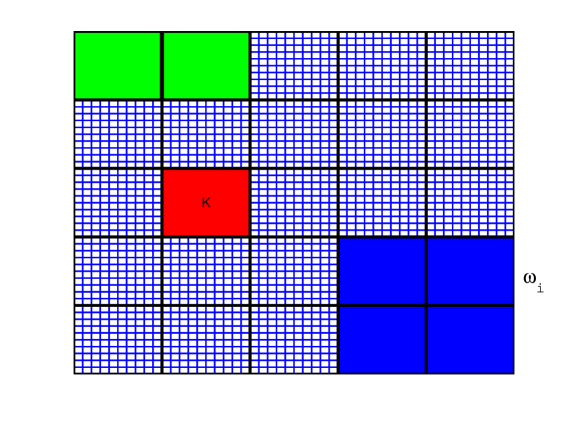
Figure 1: Illustration of coarse neighborhoods and elements. Red designates a coarse element. Green designates two neighboring elements that share a common face (used to construct test functions). Blue designates the union of all coarse elements that share a common vertex (used to construct trial functions).

2.1 Coarse-grid description

Next, we introduce some notation. We use $\mathcal{T}^{H}$ to denote a conforming partition of the computational domain $D$. The set $\mathcal{T}^{H}$ is called the coarse grid and the elements of $\mathcal{T}^{H}$ are called coarse elements. Moreover, $H>0$ is the coarse mesh size. We only consider rectangular coarse elements to simplify the discussion and illustrations. The methodology presented can be easily extended to coarse elements with more general geometries. Let $N$ be the number of nodes in the coarse grid $\mathcal{T}^{H}$, and let $\{x_{i}\,|\,1\leq i\leq N\}$ be the set of nodes in the coarse grid (or coarse nodes for short). For each coarse node $x_{i}$, we define a coarse neighborhood $\omega_{i}$ by

$$\omega_{i}=\bigcup\{K_{j}\in\mathcal{T}^{H};\leavevmode\nobreak\ \leavevmode\nobreak\ \leavevmode\nobreak\ x_{i}\in\overline{K}_{j}\}.$$ (5)

That is, $\omega_{i}$ is the union of all coarse elements $K_{j}\in\mathcal{T}^{H}$ having the coarse node $x_{i}$ (blue region in Figure 1). We use two neighboring elements sharing a common face to construct the test functions. An example of this region is depicted in green in Figure 1.

3 Generalized Multiscale Finite Element Method for Petrov-Galerkin Approximations

In this section, we discuss the construction of the multiscale basis functions for the trial space $V$ and the test space $W$. In particular, we show that one needs a good approximation for $w_{h}$ in order to achieve discrete stability. We start by introducing some notation and formulating the multiscale Petrov-Galerkin framework we solve. We introduce the snapshot space and then the local spectral decomposition used to construct the multiscale basis functions.

To simplify notations, we let

$$Au:=-\nabla\cdot(\kappa\nabla u)+b\cdot\nabla u,$$

and

$$A^{*}u:=-\nabla\cdot(\kappa\nabla u)-\nabla\cdot(b\,u).$$

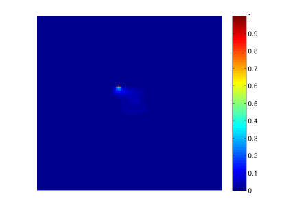
(a) Trial snapshot basis

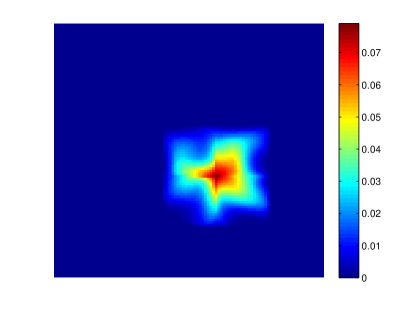
(b) Offline trial basis

Figure 2: A trial snapshot basis and the resulting offline trial basis for a given coarse block.

3.1 Construction of the multiscale trial space

3.1.1 Snapshot space

We solve a local problem with specifically designed boundary conditions to construct the snapshot basis functions. For each coarse neighborhood $\omega_{l}$, we define a set of snapshot functions $\phi_{i,l}^{snap}$ such that

$$A(\phi_{i,l}^{snap}):=-\nabla\cdot(\kappa\nabla\phi_{i,l}^{snap})+b\cdot\nabla\phi_{i,l}^{snap} =0, \text{in }\omega_{l},$$

$$\phi_{i,l}^{snap}|_{\omega_{l}}(x_{j}) =\delta_{ij}, \text{on }\partial\omega_{l},$$

where $\delta_{ij}$ is the discrete delta function defined on $\partial\omega_{l}$ with respect to the fine grid. The local snapshot space for the trial space is defined by $V^{snap}(\omega_{l})=\text{span}\{\phi_{i,l}^{snap}\}$. The snapshot functions and multiscale basis functions (offline space) are defined in the union of coarse elements that share a common vertex (Figure 1 shows a schematic representation of the grid while Figure 2 shows a solution snapshot and a multiscale basis function). We use $\Phi_{l}^{T}$ to denote the change of basis matrix from the fine-grid space $V_{h}(\omega_{l})$ to $V^{snap}(\omega_{l})$. Here $V_{h}(\omega_{l})$ is the restriction of $V_{h}$ in $\omega_{l}$.

3.1.2 Eigenproblem

To construct the offline trial space, we solve the following eigenproblem

$$(A_{snap}^{\omega_{l}})^{T}A_{snap}^{\omega_{l}}v_{j}=\lambda_{j}M_{snap}^{\omega_{l}}v_{j},$$

where

$$A_{snap}^{\omega_{l}} =\Phi_{l}^{T}A_{h}^{\omega_{l}}\Phi_{l}$$

$$M_{snap}^{\omega_{l}} =\Phi_{l}^{T}M_{h}^{\omega_{l}}\Phi_{l}$$

and $(\lambda_{j},v_{j})$ is the $j$-th eigen-pair. In the above definition, $A_{h}^{\omega_{l}}$ and $M_{h}^{\omega_{l}}$ are the restrictions of the fine-scale stiffness matrix $A_{h}$ and the fine-scale mass matrix $M_{h}$ in $\omega_{l}$. We order the eigenvalues in increasing order and we use the first $m$ eigenfunctions as the offline trial basis functions. Specifically, we define $\xi_{l,j}=\Phi_{l}v_{j}$ and $V_{off}=\text{span}\{\chi_{l}\xi_{l,j}|1\leq j\leq m,1\leq l\leq N\}$, where $\{\chi_{l}\}$ is the partition of unity.

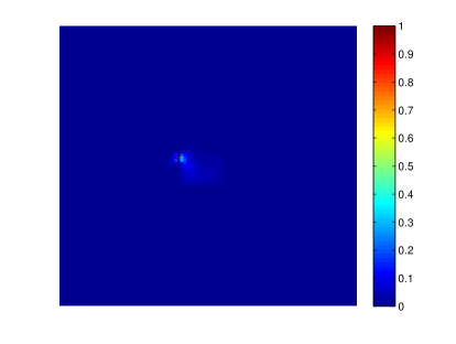
(a) Test snapshot basis for $W_{3}$

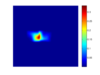
(b) Offline test basis for $W_{3}$

Figure 3: A test snapshot basis and the resulting offline test basis for a given coarse block of $W_{3}$.

3.2 Construction of the multiscale test space

3.2.1 Snapshot space

The snapshot space for the test space consists of three components, and is denoted as $W_{snap}=W_{snap}^{1}+W_{snap}^{2}+W_{snap}^{3}$. Next, we will give the constructions for $W_{snap}^{1},W_{snap}^{2}$ and $W_{snap}^{3}$. In each coarse block $K_{k}$, we define $W_{snap}^{1}(K_{k})$ as

$$W_{snap}^{1}(K_{k}):=\{\psi^{snap}\in V_{h,0}(K_{k})\;|\;A^{*}(\psi^{snap})=\xi_{l,j}\;\text{ in }K_{k}\text{ for some }\xi_{l,j}\in V_{off}\}$$

where $V_{h}(K_{k})$ is the restriction of $V_{h}$ in $K_{k}$ and $V_{h,0}(K_{k})$ is the subspace of $V_{h}(K_{k})$ containing functions that vanish on $\partial K_{k}$. The space $W_{snap}^{1}(K_{k})$ contains functions that are solution of the adjoint problem on $K_{k}$ with a source term $\xi_{l,j}$ and zero Dirichlet boundary condition. The space $W_{snap}^{1}$, is defined as $W_{snap}^{1}=\oplus_{k}W_{snap}^{1}(K_{k})$. The space $W_{snap}^{1}$ is considered as the space of multiscale bubble functions. We remark that we obtain perfect test functions (with perfect stabilization) if the above local problems are solved on the whole domain.

The second space $W_{snap}^{2}$ is defined as follows. For each coarse block $K_{k}$, we define

$$W_{snap}^{2}(K_{k}):=\{\psi^{snap}\in V_{h}(K_{k})\;|\;A^{*}(\psi^{snap})=0\;\text{ in }K_{k}\text{ and }\psi^{snap}\text{ is linear on }E\in\partial K_{k}\}.$$

The space $W_{snap}^{2}$ is defined by $W_{snap}^{2}=\oplus_{k}W_{snap}^{2}(K_{k})\cap C^{0}(\Omega)$. Note that this space is similar to the classical multiscale finite element space.

Finally, we give the definition for $W_{snap}^{3}$. For each coarse edge $E_{k}$, we define $K(E_{k})$ as the set of all coarse blocks having the edge $E_{k}$. Then, we find $\psi_{i,k}^{snap}\in V_{h}(K(E_{k}))$ such that

$$A^{*}\psi_{i,k}^{snap}:=-\nabla\cdot(\kappa\nabla\psi_{i,k}^{snap})-\nabla\cdot(b\psi_{i,k}^{snap}) =0\;\text{ in each }K\in K(E_{k}),$$

$$\psi_{i,k}^{snap}|_{E_{k}}(x_{j}) =\delta^{0}_{ij}\text{ for all }x_{j}\in E_{k},$$

$$\psi_{i,k}^{snap}|_{\partial K(E_{k})\backslash E_{k}} =0.$$

In the above system, $\delta^{0}_{ij}$ is the discrete delta function defined on $E_{k}$ with respect to the fine mesh and is zero on the boundary of $E_{k}$. Then we define $W_{snap}^{3}(E_{k})=\text{span}\{\psi_{i,k}^{snap}\}$, and $W_{snap}^{3}=\oplus_{k}W_{snap}^{3}(E_{k})$. (Figure 1 illustrates a grid and Figure 3 illustrates a snapshot solution and a multiscale basis function).

We remark that $W_{snap}=V_{h}$.

Lemma 1

For each $u\in V_{\text{{off}}}$, there exists a test function $\phi\in W_{\text{{snap}}}$ such that

$$a(v,\phi)=(u,v)_{l^{2}},\;\forall v\in V_{h}.$$ (6)

Proof: Given $u\in V_{\text{{off}}}$, we assume that $\phi\in V_{h}$ satisfies (6). For each $K\in\mathcal{T}^{H}$, we define $\phi_{\text{snap}}^{(1)}\in W_{\text{snap}}^{1}$ satisfying

$$a(v,\phi_{\text{snap}}^{(1)})=(u,v)_{l^{2}},\quad\forall v\in V_{h,0}(K),\;\forall K\in\mathcal{T}^{H}.$$

Next, we define $\phi_{\text{snap}}^{(2)}\in W_{\text{snap}}^{2}+W_{\text{snap}}^{3}$ such that

$$\phi_{\text{snap}}^{(2)}=\phi\text{ on $\partial$K},\;\forall K\in\mathcal{T}^{H}.$$

Then, we have

$$a(v,\phi-\phi_{\text{snap}}^{(1)}-\phi_{\text{snap}}^{(2)})=0,\;\forall v\in V_{h,0}(K),\;\forall K\in\mathcal{T}^{H}$$

with $\phi-\phi_{\text{snap}}^{(1)}-\phi_{\text{snap}}^{(2)}=0\text{ on $\partial$K},\;\forall K\in\mathcal{T}^{H}.$ Therefore, $\phi-\phi_{\text{snap}}^{(1)}-\phi_{\text{snap}}^{(2)}$ is a solution of the adjoint problem with zero Dirichlet boundary condition and zero source term in all $K\in\mathcal{T}^{H}$. Thus, $\phi=\phi_{\text{snap}}^{(1)}+\phi_{\text{snap}}^{(2)}\in W_{\text{snap}}.$

3.2.2 Eigenproblem

Among the three parts of the test space, the dimension of $W_{snap}^{3}$ is proportional to the number of fine-grid blocks and thus proportional to the Peclet number of the problem. Consequently, our objective is to reduce the degrees of freedom associated with $W_{snap}^{3}$. Both the dimensions of $W_{snap}^{1}$ and $W_{snap}^{2}$ are proportional to the number of coarse grid degrees of freedom. We consider two different eigenvalue problems to construct the offline test space for $W_{snap}^{3}$.

The first eigenvalue problem for $W_{snap}^{3}(E_{k})$: In this eigenvalue problem, we will use the edge values of the snapshot solutions.

$$\int_{K(E_{k})}(A^{T}v)(A^{T}\psi_{j})=\lambda\int_{E_{k}}v\psi$$

The eigenvalues go to $\infty$ as we refine the fine mesh.

The second eigenvalue problem for $W_{snap}^{3}(E_{k})$: This eigenvalue problem is motivated by [14], where we construct minimum energy snapshot solutions and perform a local spectral decomposition using the same norms. More precisely,

$$\int_{K(E_{k})}(A^{T}\tilde{v})(A^{T}\tilde{\psi_{j}})=\lambda\int_{K(E_{k})}(A^{T}v)(A^{T}\psi_{j})$$

where $\tilde{\psi}=\text{argmin}_{\tilde{\psi}\in\{v\in W_{snap}^{3}|v|_{E_{k}}=\psi|_{E_{k}}\}}\{\int_{K(E_{k})}(A^{T}\tilde{\psi})(A^{T}\tilde{\psi})\}$. In this case, the eigenvalues are always smaller than $1$.

We will arrange the eigenvalues of the above spectral problems in increasing order, and choose the first $L_{k}$ eigenfunctions as the offline test basis functions. The span of these basis functions is denoted as $W_{off}^{3}$. The final test space $W_{off}$ is defined by $W_{snap}^{1}\oplus W_{snap}^{2}\oplus W_{off}^{3}$.

3.3 Global coupling

We can use the above trial and test spaces to get a reduced system for the multiscale solution. In particular, the multiscale solution is computed by solving

$$\left(\begin{array}[]{cc}\Theta^{T}A_{h}A_{h}^{T}\Theta&\Theta^{T}A_{h}\Xi\\ \Xi^{T}A_{h}^{T}\Theta&0\end{array}\right)\left(\begin{array}[]{c}w_{ms}\\ u_{ms}^{PG}\end{array}\right)=\left(\begin{array}[]{c}\Theta^{T}f_{h}\\ 0\end{array}\right).$$ (7)

The columns of $\Theta$ consist of the computed multiscale test functions while the columns of $\Xi$ consist of the computed multiscale trial functions.

3.4 Discussion

Next, we discuss the approximation properties for the test space and how the definition of this space affects the discrete stability of the resulting method. To simplify the discussion, we introduce some notation. Let $N$ and $M$ be the dimensions for the test and trial spaces, respectively. Thus, we can write

$$\left(\begin{array}[]{cc}\Theta_{N}^{T}A_{h}A_{h}^{T}\Theta_{N}&\Theta_{N}^{T}A_{h}\Xi_{M}\\ \Xi_{M}^{T}A^{T}_{h}\Theta_{N}&0\end{array}\right)\left(\begin{array}[]{c}w_{N,M}\\ u_{N,M}^{PG}\end{array}\right)=\left(\begin{array}[]{c}\Theta_{N}^{T}f_{h}\\ 0\end{array}\right).$$ (8)

For simplicity, we denote by $\Theta_{\infty}$ the snapshot matrix that contains all snapshot vectors in the test space and similarly for the trial space $\Xi_{\infty}$. Therefore, the following statements are true:

• $w_{\infty,\infty}=0$.

• $u_{\infty,M}$ is a projection of $u_{\infty,\infty}$ onto $\Xi_{M}$

  $$u_{\infty,M}=\Pi_{\Xi_{M}}u_{\infty,\infty}.$$

• Our objective is to find the smallest possible $N$ and $M_{0}$, such that $\|u^{PG}_{N,M}-u^{PG}_{\infty,\infty}\|\preceq\|u^{PG}_{\infty,\infty}-u^{PG}_{\infty,M}\|$ for any $M$, when $M>M_{0}$.

• The inf-sup condition for our discrete saddle-point problem can be written as

  $$\sup_{\Theta}\frac{\Theta_{N}^{T}A_{h}\Xi_{M}}{(\Theta_{N}^{T}A_{h}A_{h}^{T}\Theta_{N})^{1/2}}\geq C_{infsup}(\Xi_{M}^{T}M\Xi_{M})^{1/2}.$$ (9)

  The inf-sup condition implies that

  $$C_{infsup}=\inf_{u=\Xi_{M}q}\frac{\|\Pi_{A^{T}\Theta_{N}}(u)\|_{l^{2}}}{\|u\|_{l^{2}}}.$$

  Next, we take $u=A^{T}z$. Then, the projection of $u$ onto $A^{T}\Theta_{N}$ is

  $$\Pi_{A^{T}\Theta_{N}}(u) =A^{T}\Theta_{N}((A^{T}\Theta_{N})^{T}A^{T}\Theta_{N})^{-1}(A^{T}\Theta_{N})^{T}A^{T}z$$

  $$=A^{T}\Theta_{N}(\Theta_{N}^{T}AA^{T}\Theta_{N})^{-1}\Theta_{N}^{T}AA^{T}z.$$ (10)

  We define the $\Theta$ projection in the $B$ norm to be

  $$\Pi_{\Theta,B}(z)=\Theta(\Theta^{T}B\Theta)^{-1}\Theta^{T}Bz.$$

  Thus,

  $$\|\Pi_{A^{T}\Theta_{N}}(u)\|^{2} =z^{T}AA^{T}\Theta_{N}(\Theta_{N}^{T}AA^{T}\Theta_{N})^{-1}\Theta_{N}^{T}AA^{T}\Theta_{N}(\Theta_{N}^{T}AA^{T}\Theta_{N})^{-1}\Theta_{N}^{T}AA^{T}z$$

  $$=z^{T}AA^{T}\Theta_{N}(\Theta_{N}^{T}AA^{T}\Theta_{N})^{-1}\Theta_{N}^{T}AA^{T}z$$

  $$=\|\Pi_{\Theta_{N},AA^{T}}(z)\|_{AA^{T}}^{2}.$$ (11)

  Also,

  $$\|u\|_{l^{2}}=\|z\|_{AA^{T}}.$$

  Thus,

  $$C_{infsup}=\inf_{u=A^{T}z,u=\Xi_{M}q}\frac{\|\Pi_{\Theta_{N},AA^{T}}(z)\|_{AA^{T}}}{\|z\|_{AA^{T}}}.$$ (12)

  If the inf-sup is satisfied, then we have

  $$\|w_{N,M}-w_{\infty,\infty}\|+\|u^{PG}_{N,M}-u^{PG}_{\infty,\infty}\| \preceq\|\widehat{w}_{N,M}-w_{\infty,\infty}\|+\|\widehat{u^{PG}}_{N,M}-u^{PG}_{\infty,\infty}\|$$

  $$=0+\|{u^{PG}}_{\infty,M}-u^{PG}_{\infty,\infty}\|.$$ (13)

  From here, we have

  $$\begin{split}\|w_{\infty,M}-0\|+\|u^{PG}_{\infty,M}-u^{PG}_{\infty,\infty}\|\preceq\|\widehat{u^{PG}}_{\infty,M}-u^{PG}_{\infty,\infty}\|.\end{split}$$ (14)

  Because $N=\infty$, ${u^{PG}}_{\infty,M}=\widehat{u^{PG}}_{\infty,M}$, we get

  $$\|w_{\infty,M}\|\preceq\|\widehat{u^{PG}}_{\infty,M}-u^{PG}_{\infty,\infty}\|.$$

• The discrete inf-sup condition can be shown if for any $z$ (e.g., $z=A^{-T}\Xi_{M}q$), there exists $z_{0}$ in the space spanned by $\Theta_{N}$ (i.e., $z_{0}=\Theta_{N}z_{r}$), such that

  $$\|z-z_{0}\|_{AA^{T}}\leq\delta\|z\|_{AA^{T}},$$ (15)

  for some $\delta<1$. In multiscale methods (in particular, in our works [14, 18]), we reduce the error in $\|z-z_{0}\|_{AA^{T}}$ by selecting appropriate multiscale spaces (as those used herein). In addition, this procedure can be done adaptively. Thus, by selecting a sufficient number of multiscale basis functions, we can reduce the error $\|z-z_{0}\|_{AA^{T}}$ and can achieve the stability sought. We do not have rigorous error estimates, but study this problem numerically. We emphasize that we need good approximation properties in the test space (as in [24]), which is due to the primal formulation and the choice of $z$ in (10).

3.5 Online test basis construction (residual-driven correction)

One can use residual information to construct online basis functions. Online basis functions use global information and thus accelerate the convergence. In [14], we discuss the online basis construction for flow equations using a mixed formulation. We use the local residual to construct an online basis function locally in each non-overlapping coarse grid region $\omega_{i}.$

The offline solution in the fine-scale test space $(w_{\infty,M},u_{\infty,M})\in V_{h}\times V_{off}$ satisfies

$$\left(\begin{array}[]{cc}A_{h}A_{h}^{T}&A_{h}\Xi_{M}\\ \Xi^{T}_{M}A_{h}^{T}&0\end{array}\right)\left(\begin{array}[]{c}w_{\infty,M}\\ u_{\infty,M}\end{array}\right)=\left(\begin{array}[]{c}f_{h}\\ 0\end{array}\right)$$ (16)

and the multiscale solution $(w_{N,M},u_{N,M})\in W_{off}\times V_{off}$ satisfies

$$\left(\begin{array}[]{cc}\Theta^{T}_{N}A_{h}A_{h}^{T}\Theta_{N}&\Theta^{T}_{N}A_{h}\Xi_{M}\\ \Xi^{T}_{M}A_{h}^{T}\Theta_{N}&0\end{array}\right)\left(\begin{array}[]{c}w_{N,M}\\ u_{N,M}\end{array}\right)=\left(\begin{array}[]{c}\Theta^{T}_{N}f_{h}\\ 0\end{array}\right).$$ (17)

The above motivates the following local residual operator $R_{i}$, which is defined as $R_{i}:V_{h}(\omega_{i})\rightarrow\mathbb{R}$ is defined by

$$R_{i}(v)=v^{T}\Big{(}(A_{h}A_{h}^{T})^{(i)}\Theta_{N}w_{N,M}+(A_{h})^{(i)}\Xi_{M}u_{N,M}-f_{h}\Big{)}$$

and the local residual norm, $\|R_{i}\|$ is defined by

$$\|R_{i}\|=\sup_{v\in V_{h}(\omega_{i})}\cfrac{|R_{i}(v)|}{\sqrt{v^{T}(A_{h}A_{h}^{T})^{(i)}v}}\,,$$

where $(A_{h}A_{h}^{T})^{(i)}$ and $A_{h}^{(i)}$ are local sub-matrices of $A_{h}A_{h}^{T}$ and $A_{h}$ which correspond to the coarse grid subdomain $\omega_{i}$. Next, we use the local residual to construct the local test basis, $\phi_{on}^{(i)}\in V_{h}(\omega_{i})$ such that

$$v^{T}(A_{h}A_{h}^{T})^{(i)}\phi_{on}^{(i)}=R_{i}(v),\quad\forall v\in V_{h}(\omega_{i}).$$

In [14], we show that if online basis functions are constructed using the second eigenvalue problem, then the error will decrease at a rate $(1-\min_{E}\Lambda_{\min}^{E})$, where $\Lambda_{\min}^{E}$ is the minimum of the eigenvalues of the spectral problem defined on $W_{snap}^{3}(E)$ corresponding to eigenfunctions not chosen as basis. Consequently, using online basis functions, we can achieve the discrete inf-sup stability in one iteration provided $\min_{E}\Lambda_{\min}^{E}>0$.

3.5.1 Online test basis enrichment algorithm

First, we choose an offline trial space, $V_{\text{off}}$ and an initial offline test space, $W^{(1)}_{\text{off}}$, by fixing the number of basis functions for each coarse neighborhood. Next, we construct a sequence of online test spaces $W^{(m)}_{\text{off}}$ and compute the multiscale solution $(w^{(m)}_{\text{ms}},u^{(m)}_{\text{ms}})$ by solving equation (17). The test space is constructed iteratively for $m=1,2,3,\dots,$ by the following algorithm:

1. Find the multiscale solution in the current space. Solve for $(w^{(m)}_{\text{ms}},u^{(m)}_{\text{ms}})\in W^{(m)}_{\text{off}}\times V_{\text{off}}$ such that

   $$\left(\begin{array}[]{cc}(\Theta^{(m)}_{\text{off}})^{T}A_{h}A_{h}^{T}\Theta^{(m)}_{\text{off}}&(\Theta^{(m)}_{\text{off}})^{T}A_{h}\Pi^{(m)}_{\text{off}}\\ (\Xi^{(m)}_{\text{off}})^{T}A_{h}^{T}\Theta^{(m)}_{\text{off}}&0\end{array}\right)\left(\begin{array}[]{c}w^{(m)}_{\text{ms}}\\ u^{(m)}_{\text{ms}}\end{array}\right)=\left(\begin{array}[]{c}(\Theta^{(m)}_{\text{off}})^{T}f_{h}\\ 0\end{array}\right).$$

2. For each coarse region $\omega_{i}$, compute the online basis, $\phi^{(i)}_{\text{on}}\in V_{h}(\omega_{i})$ such that

   $$v^{T}(A_{h}A_{h}^{T})^{(i)}\phi_{on}^{(i)}=R_{i}(v),\quad\forall v\in V_{h}(\omega_{i}).$$

3. Enrich the test space by setting

   $$W^{(m+1)}_{\text{off}}=W^{(m)}_{\text{off}}+\text{span}\{\phi^{(i)}_{\text{on}}\}.$$

We remark that in each iteration, we perform the above procedure on non-overlapping coarse neighborhoods, see [14].

4 Numerical Results

In this section, we present representative numerical examples. In all our examples, $\{\chi_{i}\}$ is a multiscale partition of unity. In each coarse space, we compare the $l_{2}$ projection error and the $l_{2}$ error for the multiscale solution. For simplicity, we refer to “the multiscale error” as the error between the multiscale solution and the exact solution, and “the projection error” as the error between the exact solution and its $l_{2}$ projection onto the span of the coarse trial space. We also assume $\kappa$ is a constant and $b$ is a multiscale field. In particular, the velocity fields contain oscillations and cells (eddies, separatrices and/or layers) within a single coarse block of the discretization and, thus, we do not have a single streamline direction per coarse block. Fully resolved velocity solutions are shown in Figures 4 to 6 and in Figure 8. The method can easily handle multiscale diffusion coefficients. The fine-grid problem is always chosen such that the local Peclet number is about $1$ ensuring a stable fine discretization. All coarse discretizations have a Peclet number at least an order of magnitude larger than $1$. We analyze the performance of the trial and test spaces proposed in the previous section. We pay special attention to the effect of eigenvalue problem on the performance of the discrete system and discuss this for each example.

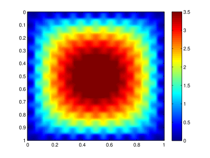
(a) $\alpha=2$

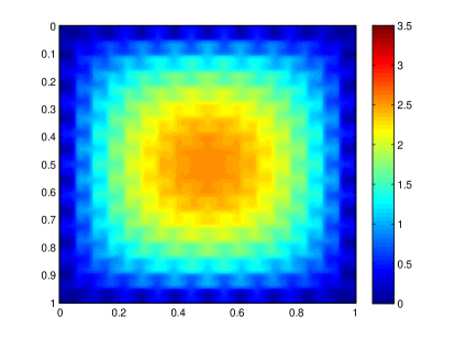
(b) $\alpha=4$

Figure 4: Reference solutions for Example 1.

Example 1

These first numerical examples are defined by the following diffusion and convection coefficients and right-hand side,

$$\kappa =\dfrac{1}{100},$$

$$b =\alpha\left(\begin{array}[]{c}+\sin(18\pi x)\cos(18\pi y)\\ -\cos(18\pi x)\sin(18\pi y)\end{array}\right),$$

$$f =1.$$

#basis	$L_{2}$ (projection error)
(trial, test)	Eigenproblem 1		Eigenproblem 2
	$\alpha=2$	$\alpha=4$	$\alpha=2$	$\alpha=4$
(1,1)	8.56%	7.06%	11.94%	9.60%
(1,3)	3.22%	4.96%	4.74%	4.48%
(1,5)	2.85%	4.74%	2.90%	5.02%
(1,7)	2.85%(2.85%)	3.64%(3.52%)	2.85%(2.85%)	3.55%(3.52%)
(3,1)	9.00%	7.58%	11.95%	8.86%
(3,3)	3.12%	5.22%	5.01%	3.96%
(3,5)	2.61%	3.96%	2.70%	4.83%
(3,7)	2.60%(2.60%)	3.41%(3.21%)	2.61%(2.60%)	3.25%(3.21%)
(5,1)	8.65%	7.88%	12.80%	9.08%
(5,3)	2.72%	4.97%	4.69%	3.35%
(5,5)	2.31%	3.62%	2.37%	3.99%
(5,7)	2.31%(2.31%)	2.89%(2.77%)	2.31%(2.31%)	2.79%(2.77%)

Table 1: Errors for test space derived using Eigenproblems 1 and 2 for Example 1. Coarse and fine mesh sizes are $H=1/10$ and $h=1/200$, respectively. The projection errors are in parentheses.

This velocity field has a cellular structure with several eddies and separatices. In the simulations $\alpha$ takes values of 2 and 4. Figure 4 depicts well-resolved fine-scale solutions for the chosen values of $\alpha$. In both cases, we take the coarse mesh size to be $H=1/10$, while the fine mesh size to be $h=1/200$.

#basis test	$\min\{\lambda_{L_{i}+1}\}$
	$\alpha=2$	$\alpha=4$
1	0.3445	0.3693
3	0.7273	0.7707
5	0.9542	0.9514
7	0.9908	0.9919

Table 2: Minimum eigenvalue for the test space constructed using the Eigenproblem 2 (minimal energy test functions) for Example 1. Coarse and fine mesh sizes are $H=1/10$ and $h=1/200$, respectively.

Table 1 shows the impact of increasing the number of coarse basis functions as well as how the system converges as we increase the number of test functions included per coarse block edge. The table shows the evolution of the multiscale error as we increase the number of test functions for different numbers of trial functions in each coarse block. Each column is labeled by its corresponding value of $\alpha$. Table 1 shows the performance of the reduced-dimensional test space constructed using the first and second eigenvalue problems we describe in Section 3.2.2. This table shows that $7$ test functions per edge of the coarse mesh are enough to deliver similar multiscale and projection errors irrespective of $\alpha$ (i.e., coarse scale Peclet number) and the number of coarse basis functions used in each coarse block. In fact, these errors are similar even when the number of test functions is $5$. Table 2 shows the evolution of the minimum eigenvalue for the test space constructed using the Eigenproblem 2 (minimal energy test functions) of Section 3.2.2. As it follows from the theory, for a rich enough test space with a sufficient number of multiscale test functions, multiscale and projection errors converge. The eigenvalue behavior shown in Table 2 and the convergence shown in Table 1 verifies that when the minimum eigenvalue is close to $1$, the multiscale error converges to the projection error.

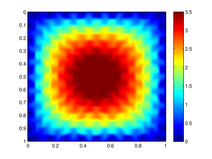
(a) $\alpha=2$

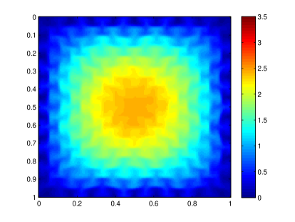
(b) $\alpha=4$

Figure 5: Reference solutions for Example 2.

Example 2

We consider the following right-hand side, and diffusion and convection coefficients:

$$\kappa =1/100,$$

$$b =\alpha\left(\begin{array}[]{c}+\sin(18\pi x)\cos(18\pi y)+\delta\cos(18\sqrt{2}\pi x)\sin(18\sqrt{2}\pi y)\\ -\cos(18\pi x)\sin(18\pi y-\delta\sin(18\sqrt{2}\pi x)\sin(18\sqrt{2}\pi y)\end{array}\right),$$

$$f =1.$$

This velocity field has a cellular structure with eddies and channels, as can be seen in the fine-scale solutions depicted in Figure 5. These channels introduce global effects. $\alpha$ takes values of 2 and 4, as in our previous example. $\delta$ takes value of $\sqrt{2}/4$. For both cases, we take the coarse mesh size to be $H=1/10$, while the fine mesh size to be $h=1/200$.

#basis	$L_{2}$ (projection error)
(trial, test)	Eigenproblem 1		Eigenproblem 2
	$\alpha=2$	$\alpha=4$	$\alpha=2$	$\alpha=4$
(1,1)	9.49%	8.57%	12.27%	9.99%
(1,3)	3.11%	5.04%	4.62%	4.22%
(1,5)	2.90%	4.73%	2.95%	4.62%
(1,7)	2.90%(2.90%)	3.87%(3.67%)	2.90%(2.90%)	3.70%(3.67%)
(3,1)	10.04%	9.09%	12.35%	9.33%
(3,3)	2.97%	4.50%	5.09%	3.73%
(3,5)	2.65%	3.85%	2.75%	4.52%
(3,7)	2.65%(2.64%)	3.56%(3.33%)	2.65%(2.64%)	3.38%(3.33%)
(5,1)	9.22%	9.25%	13.37%	9.98%
(5,3)	2.67%	4.18%	4.60%	3.26%
(5,5)	2.36%	3.43%	2.42%	3.84%
(5,7)	2.36%(2.36%)	3.18%(2.84%)	2.36%(2.36%)	2.88%(2.84%)

Table 3: Errors for test space derived using Eigenproblems 1 and 2 for Example 2, with $\delta=\sqrt{2}/4$. Coarse and fine mesh sizes are $H=1/10$ and $h=1/200$, respectively. The projection errors are in parentheses.

#basis test	$\min\{\lambda_{L_{i}+1}\}$
	$\alpha=2$	$\alpha=4$
1	0.3551	0.2967
3	0.7289	0.6761
5	0.9510	0.9331
7	0.9909	0.9813

Table 4: Minimum eigenvalue for the test space constructed using the Eigenproblem 2 (minimal energy test functions) for Example 2 for $\delta=\sqrt{2}/4$. Coarse and fine mesh sizes are $H=1/10$ and $h=1/200$, respectively.

In Table 3, we increase the number of test functions and consider different numbers of trial functions for both eigenvalue problems described in Section 3.2.2. As before, we observe that for $7$ test functions, the multiscale and projection errors converge, while for $5$ test functions per edge, the errors are close. As we increase, the dimension of the coarse trial space, we observe a similar behavior. The eigenvalue behavior shows (see Table 4) that when the eigenvalue is close to $1$, the multiscale and projection errors converge.

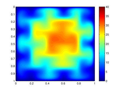
(a) $\alpha=1/1000$

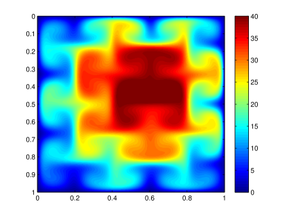
(b) $\alpha=1/2000$

Figure 6: Reference solutions for Example 3.

Example 3

#basis	$L_{2}$ (projection error)
(trial, test)	Eigenproblem 1		Eigenproblem 2
	$\alpha=1/1000$	$\alpha=1/2000$	$\alpha=1/1000$	$\alpha=1/2000$
(1,1)	9.59%	32.36%	19.09%	34.55%
(1,3)	7.84%	13.70%	15.58%	32.00%
(1,5)	7.83%	12.10%	9.10%	22.53%
(1,7)	7.83%(7.83%)	11.85%(11.48%)	7.95%(7.83%)	14.70%(11.48%)
(3,1)	6.01%	16.24%	16.70%	37.12%
(3,3)	4.89%	9.07%	7.93%	18.82%
(3,5)	4.88%	7.98%	5.33%	11.90%
(3,7)	4.88%(4.88%)	8.06%(7.58%)	4.98%(4.88%)	9.71%(7.58%)
(5,1)	4.70%	14.77%	14.00%	31.46%
(5,3)	3.74%	6.61%	4.79%	13.66%
(5,5)	3.72%	6.23%	3.80%	7.55%
(5,7)	3.72%(3.72%)	6.21%(6.15%)	3.74%(3.72%)	6.53%(6.15%)

Table 5: Errors for test space derived using Eigenproblems 1 and 2 for Example 3. Discrete parameters used are: $\alpha=1/1000$, $H=1/10$, $h=1/400$ and $\alpha=1/2000$, $H=1/10$, $h=1/800$. The projection errors are in parentheses.

#basis test	$\min\{\lambda_{L_{i}+1}\}$
	$\alpha=1/1000$	$\alpha=1/2000$
1	0.3547	0.3068
3	0.7497	0.6304
5	0.9546	0.8718
7	0.9952	0.9754

Table 6: Minimum eigenvalue for test space derived using Eigenproblem 2 for Example 3. Discrete parameters used are: $\alpha=1/1000$, $H=1/10$, $h=1/400$ and $\alpha=1/2000$, $H=1/10$, $h=1/800$.

We consider the following diffusion and convection coefficients and right-hand side.

$$\kappa =\alpha,$$

$$b =\left(\begin{array}[]{c}-\frac{\partial H}{\partial y}\vspace{.05in}\\ +\frac{\partial H}{\partial x}\end{array}\right),$$

$$f =1,$$

where

$$H=(\sin(5\pi x)\sin(6\pi y)/(60\pi))+0.005(x+y).$$

This velocity field again has a cellular structure with eddies and channels, as the fine-scale solutions show in Figure 6. In this example, $\alpha$ is a diffusion coefficient and we take $\alpha=1/1000$ and $\alpha=1/2000$. For both cases, we take the coarse mesh size to be $H=1/10$, while the fine mesh sizes are set to $h=1/400$ and $h=1/800$ for $\alpha=1/1000$ and $\alpha=1/2000$, respectively.

Tables 5 and 6 show a similar behavior to the one discussed in the previous two examples. That is, table 5 shows that if only one test function is chosen for $\alpha=1/2000$, the error is about $35$% (when the number of test functions coarse edge is $1$ and the number of trial functions per coarse block is $1$). These errors rapidly drop to about the projection error as we increase the dimension of the test space. Similar behavior is observed for both eigen-constructions of the test space as we refine the coarse trial space.

#basis (trial, test)	$L_{2}$ (projection error)
(1,1)	20.12%
(1,3)	11.25%
(1,5)	4.03%
(1,7)	3.93%(3.93%)
(3,1)	19.99%
(3,3)	13.02%
(3,5)	3.31%
(3,7)	3.23%(3.23%)
(5,1)	13.93%
(5,3)	9.14%
(5,5)	2.90%
(5,7)	2.74%(2.70%)

Table 7: Errors for test space derived using Eigenproblem 2 for Example 4. Coarse and fine mesh sizes are $H=1/10$ and $h=1/200$, respectively. The projection errors are in parentheses.

Example 4

As we remove the eddies from the flow field and make the flow more channelized, the multiscale error grows. To expose this behavior, we take the velocity field to be

$$\kappa =1,$$

$$b =200\left(\begin{array}[]{c}\sin(18\sqrt{2}\pi y)\\ 0\end{array}\right),$$

$$f =1,$$

which corresponds to solving the flow equations with a channelized permeability field. The numerical results are presented in Table 7 (the mesh sizes for the coarse and fine spaces are $H=1/10$ and $h=1/200$). We observe that the multiscale error is $20.12$% for one trial function per coarse block and one test function per coarse interface, while the error reduces to the projection error of $3.93$% when we select $7$ test functions interface. As before, for $5$ trial functions per coarse block, it takes $7$ test functions per coarse interface to reduce the error to the projection error from $13.93$%. For this discrete problem setup, the smallest eigenvalue is $0.9952$ for $7$ test functions per edge when minimal energy functions are used (Eigenproblem 2 in Section 3.2.2).

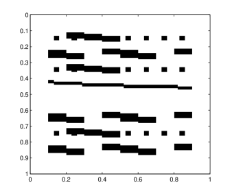
Figure 7: Permeability field used to compute the transport velocity field in Example 5. The black region corresponds to the permeability $500$ and the white region corresponds to the permeability $1$.

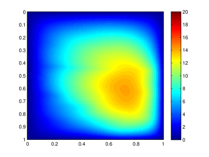
(a) $\alpha=1/250$

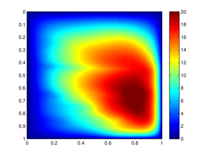
(b) $\alpha=1/500$

Figure 8: Reference solutions for Example 5.

Example 5

#basis	$L_{2}$ (projection error)
(trial, test)	Eigenproblem 1		Eigenproblem 2
	$\alpha=1/250$	$\alpha=1/500$	$\alpha=1/250$	$\alpha=1/500$
(1,1)	2.11%	4.64%	2.24%	4.56%
(1,3)	2.08%	4.59%	2.09%	4.24%
(1,5)	2.07%	4.45%	2.07%	4.15%
(1,7)	2.07%(2.07%)	4.23%(4.04%)	2.07%(2.07%)	4.19%(4.04%)
(3,1)	1.01%	1.98%	1.68%	3.57%
(3,3)	0.99%	1.93%	1.07%	2.36%
(3,5)	0.99%	1.93%	1.00%	2.05%
(3,7)	0.99%(0.99%)	1.93%(1.91%)	0.99%(0.99%)	2.01%(1.91%)
(5,1)	0.85%	1.70%	1.64%	4.12%
(5,3)	0.75%	1.44%	0.84%	1.91%
(5,5)	0.75%	1.44%	0.76%	1.53%
(5,7)	0.75%(0.75%)	1.44%(1.42%)	0.75%(0.75%)	1.49%(1.42%)

Table 8: Errors for test space derived using Eigenproblems 1 amd 2 for Example 5. Discrete parameters used are: $\alpha=1/250$, $H=1/10$, $h=1/200$ and $\alpha=1/500$, $H=1/10$, $h=1/400$. The projection errors are in parentheses.

We consider the following diffusion and convection coefficients, and right-hand side.

$$\kappa =\alpha,$$

$$b =\kappa\nabla p$$

$$f =1,$$

where the velocity field solves this flow equation

$$-\nabla\cdot(\kappa\nabla p) =0$$

$$p|_{\partial\Omega} =xy$$

Figure 7 shows the permeability field used in the above equation. The resulting velocity field contains channels with variable velocity in each coarse region. Figure 8 shows the fine-scale structure of the fully resolved velocity field. In this case $\alpha$ is a diffusion coefficient and takes values $1/250$ and $1/500$. In both cases, we take the coarse mesh size is set to $H=1/10$, while the fine mesh sizes are $h=1/200$ and $h=1/400$ for $\alpha=1/250$ and $\alpha=1/500$, respectively.

Tables 8 and 9 show a similar behavior to that observed in the prior examples. That is, the multiscale error converges to the projection error as we increase the number of test functions per coarse edge for either eigenvalue problem and for any number of coarse functions in each coarse block.

#basis test	$\min\{\lambda_{L_{i}+1}\}$
	$\alpha=1/1000$	$\alpha=1/2000$
1	0.4106	0.3544
3	0.8592	0.7583
5	0.9828	0.9535
7	0.9985	0.9919

Table 9: Minimum eigenvalue for test space derived using Eigenproblem 2 for Example 3. Discrete parameters used are:$\alpha=1/250,H=1/10,h=1/200$ and $\alpha=1/500,H=1/10,h=1/400$

#basis	#iter	Eigenproblem 1		Eigenproblem 2
(trial, test)		$\alpha=2$	$\alpha=4$	$\alpha=2$	$\alpha=4$
	0	8.56%	7.06%	11.94%	9.60%
(1,1)	1	2.89%	3.79%	2.96%	4.30%
	2	2.85%(2.85%)	3.52%(3.52%)	2.85%(2.85%)	3.52%(3.52%)
	0	3.22%	4.96%	4.74%	4.48%
(1,3)	1	2.85%	3.54%	2.86%	3.63%
	2	2.85%(2.85%)	3.52%(3.52%)	2.85%(2.85%)	3.52%(3.52%)
	0	8.65%	7.88%	12.80%	9.08%
(5,1)	1	2.33%	2.97%	2.58%	3.29%
	2	2.31%(2.31%)	2.77%(2.77%)	2.32%(2.31%)	2.78%(2.77%)
	0	2.72%	4.97%	4.69%	3.35%
(5,3)	1	2.31%	2.79%	2.33%	2.81%
	2	2.31%(2.31%)	2.77%(2.77%)	2.31%(2.31%)	2.77%(2.77%)

Table 10: Error evolution as online basis functions are added to the system (test space derived using Eigenproblems 1 and 2 for Example 1). Coarse and fine mesh sizes are $H=1/10$ and $h=1/200$, respectively. The projection errors are in parentheses.

4.1 Numerical Result for online test basis enrichment

In this section, we present some numerical results, which use online test basis functions to stabilize the system. In Table 10, we show the convergence history for the online test basis enrichment for Example 1, while in Table 11, we show the convergence history of the online test basis enrichment for Example 4. In these two cases, with only one iteration, the multiscale error becomes similar to the projection error. In the second iteration, the multiscale error converges to the projection error.

#basis	#iter
(trial, test)
	0	20.12%
(1,1)	1	3.93%
	2	3.92%(3.92%)
	0	11.15%
(1,3)	1	3.92%
	2	3.92%(3.92%)
	0	13.93%
(5,1)	1	3.24%
	2	2.72%(2.70%)
	0	9.14%
(5,3)	1	2.74%
	2	2.70%(2.70%)

Table 11: Error evolution as online basis functions are added to the system (test space derived using Eigenproblem 2 for Example 4). Coarse and fine mesh sizes are $H=1/10$ and $h=1/200$, respectively. The projection errors are in parentheses.

5 Conclusions

In this paper, we study multiscale methods for convection-dominated diffusion with heterogeneous convective velocity fields. This stabilization generalizes the approaches described in [29] to multiscale problems. To construct this stabilization we reformulate overall problem in mixed form. The auxiliary variable we introduce plays the role of the test function. We describe the multiscale spaces we use for the test and trial spaces, which are built using GMsFEM framework. First, we construct snapshots spaces. For the test variable, we propose local snapshot spaces. Furthermore, we propose a local spectral decomposition following our recent work [14], where we consider minimum energy snapshot functions. We discuss the discrete stability of the system and its relation to the approximation properties of the velocity field. The resulting approximation error is minimized within our multiscale framework by selecting a few multiscale basis functions. Our numerical results show that we can stabilize the system using a few test functions for a given trial space. We describe and analyze several relevant numerical examples that validate our theoretical results.

References

- [1] I Akkerman, Y Bazilevs, VM Calo, TJR Hughes, and S Hulshoff. The role of continuity in residual-based variational multiscale modeling of turbulence. Computational Mechanics, 41(3):371–378, 2008.
- [2] M Alotaibi, VM Calo, Y Efendiev, JC Galvis, and M Ghommem. Global–local nonlinear model reduction for flows in heterogeneous porous media. Computer Methods in Applied Mechanics and Engineering, 292:122–137, 2015.
- [3] T. Arbogast. Analysis of a two-scale, locally conservative subgrid upscaling for elliptic problems. SIAM J. Numer. Anal., 42(2):576–598 (electronic), 2004.
- [4] JW Barrett and KW Morton. Approximate symmetrization and Petrov-Galerkin methods for diffusion-convection problems. Computer Methods in Applied Mechanics and Engineering, 45(1):97–122, 1984.
- [5] Y Bazilevs, VM Calo, JA Cottrell, TJR Hughes, A Reali, and G Scovazzi. Variational multiscale residual-based turbulence modeling for large eddy simulation of incompressible flows. Computer Methods in Applied Mechanics and Engineering, 197(1):173–201, 2007.
- [6] Y Bazilevs, C Michler, VM Calo, and TJR Hughes. Isogeometric variational multiscale modeling of wall-bounded turbulent flows with weakly enforced boundary conditions on unstretched meshes. Computer Methods in Applied Mechanics and Engineering, 199(13):780–790, 2010.
- [7] PB Bochev and MD Gunzburger. Finite element methods of least-squares type. SIAM review, 40(4):789–837, 1998.
- [8] PB Bochev and MD Gunzburger. Least-squares finite element methods, volume 166. Springer Science & Business Media, 2009.
- [9] A Buffa, TJR Hughes, and G Sangalli. Analysis of a multiscale discontinuous Galerkin method for convection-diffusion problems. SIAM Journal on Numerical Analysis, 44(4):1420–1440, 2006.
- [10] VM Calo, Y Efendiev, J Galvis, and M Ghommem. Multiscale empirical interpolation for solving nonlinear PDEs. Journal of Computational Physics, 278:204–220, 2014.
- [11] VM Calo, Y Efendiev, J Galvis, and G Li. Randomized oversampling for generalized multiscale finite element methods. http://arxiv.org/pdf/1409.7114.pdf, 2014.
- [12] VM Calo, Y Efendiev, and JC Galvis. A note on variational multiscale methods for high-contrast heterogeneous porous media flows with rough source terms. Advances in Water Resources, 34(9):1177–1185, 2011.
- [13] VM Calo, Y Efendiev, and JC Galvis. Asymptotic expansions for high-contrast elliptic equations. Mathematical Models and Methods in Applied Sciences, 24(03):465–494, 2014.
- [14] HY Chan, ET Chung, and Y Efendiev. Adaptive mixed GMsFEM for flows in heterogeneous media. arXiv preprint arXiv:1507.01659, 2015.
- [15] J Chan, N Heuer, T Bui-Thanh, and L Demkowicz. A robust DPG method for convection-dominated diffusion problems ii: Adjoint boundary conditions and mesh-dependent test norms. Computers & Mathematics with Applications, 67(4):771–795, 2014.
- [16] C.-C. Chu, I. G. Graham, and T.-Y. Hou. A new multiscale finite element method for high-contrast elliptic interface problems. Math. Comp., 79(272):1915–1955, 2010.
- [17] Eric T Chung, Yalchin Efendiev, and Wing Tat Leung. An adaptive generalized multiscale discontinuous galerkin method (GMsDGM) for high-contrast flow problems. arXiv preprint arXiv:1409.3474, 2014.
- [18] ET Chung, Y Efendiev, and CS Lee. Mixed generalized multiscale finite element methods and applications. Multiscale Modeling & Simulation, 13(1):338–366, 2015.
- [19] ET Chung, Y Efendiev, and WT Leung. Residual-driven online generalized multiscale finite element methods. To appear in J. Comput. Phys.
- [20] ET Chung, Y Efendiev, and WT Leung. An online generalized multiscale discontinuous Galerkin method (GMsDGM) for flows in heterogeneous media. arXiv preprint arXiv:1504.04417, 2015.
- [21] ET Chung, Y Efendiev, and G Li. An adaptive GMsFEM for high-contrast flow problems. Journal of Computational Physics, 273:54–76, 2014.
- [22] ET Chung, Y Efendiev, G Li, and M Vasilyeva. Generalized multiscale finite element methods for problems in perforated heterogeneous domains. Applicable Analysis, to appear, 2015.
- [23] R Codina. Comparison of some finite element methods for solving the diffusion-convection-reaction equation. Computer Methods in Applied Mechanics and Engineering, 156(1):185–210, 1998.
- [24] W Dahmen, C Plesken, and G Welper. Double greedy algorithms: reduced basis methods for transport dominated problems. ESAIM: Mathematical Modelling and Numerical Analysis, 48(03):623–663, 2014.
- [25] L Demkowicz and J Gopalakrishnan. A primal DPG method without a first-order reformulation. Computers & Mathematics with Applications, 66(6):1058–1064, 2013.
- [26] L Demkowicz, J Gopalakrishnan, and AH Niemi. A class of discontinuous Petrov-Galerkin methods. Part III: adaptivity. Applied numerical mathematics, 62(4):396–427, 2012.
- [27] L Demkowicz and N Heuer. Robust DPG method for convection-dominated diffusion problems. SIAM Journal on Numerical Analysis, 51(5):2514–2537, 2013.
- [28] L Demkowicz and JT Oden. An adaptive characteristic Petrov-Galerkin finite element method for convection-dominated linear and nonlinear parabolic problems in two space variables. Computer Methods in Applied Mechanics and Engineering, 55(1):63–87, 1986.
- [29] LF Demkowicz and J Gopalakrishnan. An overview of the discontinuous Petrov Galerkin method. In Recent Developments in Discontinuous Galerkin Finite Element Methods for Partial Differential Equations, pages 149–180. Springer International Publishing, 2014.
- [30] L.J. Durlofsky. Numerical calculation of equivalent grid block permeability tensors for heterogeneous porous media. Water Resour. Res., 27:699–708, 1991.
- [31] W. E and B. Engquist. Heterogeneous multiscale methods. Comm. Math. Sci., 1(1):87–132, 2003.
- [32] Y. Efendiev and J. Galvis. Coarse-grid multiscale model reduction techniques for flows in heterogeneous media and applications. Chapter of Numerical Analysis of Multiscale Problems, Lecture Notes in Computational Science and Engineering, Vol. 83, pages 97–125.
- [33] Y. Efendiev, J. Galvis, and T. Hou. Generalized multiscale finite element methods. Journal of Computational Physics, 251:116–135, 2013.
- [34] Y. Efendiev, J. Galvis, S. Ki Kang, and R.D. Lazarov. Robust multiscale iterative solvers for nonlinear flows in highly heterogeneous media. Numer. Math. Theory Methods Appl., 5(3):359–383, 2012.
- [35] Y Efendiev, J Galvis, R Lazarov, M Moon, and M Sarkis. Generalized multiscale finite element method. Symmetric interior penalty coupling. Journal of Computational Physics, 255:1–15, 2013.
- [36] Y Efendiev, J Galvis, G Li, and M Presho. Generalized multiscale finite element methods. Oversampling strategies. International Journal for Multiscale Computational Engineering, accepted, 2013.
- [37] Y. Efendiev, J. Galvis, and X.H. Wu. Multiscale finite element methods for high-contrast problems using local spectral basis functions. Journal of Computational Physics, 230:937–955, 2011.
- [38] Y. Efendiev and T. Hou. Multiscale Finite Element Methods: Theory and Applications. Springer, 2009.
- [39] Y. Efendiev, T. Hou, and V. Ginting. Multiscale finite element methods for nonlinear problems and their applications. Comm. Math. Sci., 2:553–589, 2004.
- [40] L. Jiang F. Chen, E. Chung. Least squares GMsFEM. 2015. in preparation.
- [41] A Fannjiang and G Papanicolaou. Convection enhanced diffusion for periodic flows. SIAM Journal on Applied Mathematics, 54(2):333–408, 1994.
- [42] J Galvis and Y Efendiev. Domain decomposition preconditioners for multiscale flows in high-contrast media. Multiscale Model. Simul., 8(4):1461–1483, 2010.
- [43] J Galvis and Y Efendiev. Domain decomposition preconditioners for multiscale flows in high contrast media: reduced dimension coarse spaces. Multiscale Model. Simul., 8(5):1621–1644, 2010.
- [44] J Galvis, G Li, and K Shi. A generalized multiscale finite element method for the Brinkman equation. Journal of Computational and Applied Mathematics, 280:294–309, 2015.
- [45] J. Galvis and J. Wei. Ensemble level multiscale finite element and preconditioner for channelized systems and applications. Journal of Computational and Applied Mathematics, 255:456–467, 2014.
- [46] M. Ghommem, M. Presho, V. M. Calo, and Y. Efendiev. Mode decomposition methods for flows in high-contrast porous media. global-local approach. Journal of Computational Physics, 253:226–238, 2013.
- [47] M-C Hsu, Y Bazilevs, VM Calo, TE Tezduyar, and TJR Hughes. Improving stability of stabilized and multiscale formulations in flow simulations at small time steps. Computer Methods in Applied Mechanics and Engineering, 199(13):828–840, 2010.
- [48] TJR Hughes. Multiscale phenomena: Green’s functions, the Dirichlet-to-Neumann formulation, subgrid scale models, bubbles and the origins of stabilized methods. Computer methods in applied mechanics and engineering, 127(1):387–401, 1995.
- [49] TJR Hughes, VM Calo, and G Scovazzi. Variational and multiscale methods in turbulence. In Mechanics of the 21st Century, pages 153–163. Springer, 2005.
- [50] TJR Hughes, G Feijoo, L Mazzei, and J Quincy. The variational multiscale method—a paradigm for computational mechanics. Comput. Methods Appl. Mech. Engrg., 166:3–24, 1998.
- [51] TJR Hughes, LP Franca, and GM Hulbert. A new finite element formulation for computational fluid dynamics: VIII. The Galerkin/least-squares method for advective-diffusive equations. Computer Methods in Applied Mechanics and Engineering, 73(2):173–189, 1989.
- [52] TJR Hughes and G Sangalli. Variational multiscale analysis: the fine-scale Green’s function, projection, optimization, localization, and stabilized methods. SIAM Journal on Numerical Analysis, 45(2):539–557, 2007.
- [53] A Masud and RA Khurram. A multiscale/stabilized finite element method for the advection–diffusion equation. Computer Methods in Applied Mechanics and Engineering, 193(21):1997–2018, 2004.
- [54] AH Niemi, NO Collier, and VM Calo. Discontinuous Petrov-Galerkin method based on the optimal test space norm for one-dimensional transport problems. Procedia Computer Science, 4:1862–1869, 2011.
- [55] AH Niemi, NO Collier, and VM Calo. Automatically stable discontinuous Petrov-Galerkin methods for stationary transport problems: Quasi-optimal test space norm. Computers & Mathematics with Applications, 66(10):2096–2113, 2013.
- [56] PJ Park and TY Hou. Multiscale numerical methods for singularly perturbed convection-diffusion equations. International Journal of Computational Methods, 1(01):17–65, 2004.
- [57] X.H. Wu, Y. Efendiev, and T.Y. Hou. Analysis of upscaling absolute permeability. Discrete and Continuous Dynamical Systems, Series B., 2:158–204, 2002.
- [58] J Zitelli, I Muga, L Demkowicz, J Gopalakrishnan, D Pardo, and VM Calo. A class of discontinuous Petrov-Galerkin methods. Part IV: The optimal test norm and time-harmonic wave propagation in 1d. Journal of Computational Physics, 230(7):2406–2432, 2011.