grayStar3 - gray no more: More physical realism and a more intuitive interface - all still in a WWW browser

Abstract

The goal of the openStar project is to turn any WWW browser, running on any platform, into a virtual star equipped with parameter knobs and instrumented with output displays that any user can experiment with using any device for which a browser is available. grayStar3 (gS3) is a major improvement upon GrayStar 2.0 (GS2), both in the physical realism of the modeling and the intuitiveness of the user interface. The code only makes use of programmability that is natively supported by all WWW browsers, and integrates scientific modeling computation in JavaScript with graphical visualization of the output in HTML. The user interface is adaptable so as to be appropriate for a large range of audiences from the high-school to the introductory post-graduate level. The modeling is physically based and all outputs are determined entirely and directly by the results of in situ physical modeling, giving the code significant generality and credibility for pedagogical applications. gS3 also models and displays the circumstellar habitable zone (CHZ) and allows the user to adjust the greenhouse effect and albedo of the planet. In its default mode the code is guaranteed to return a result within a few second of wall-clock time on any device, including low power portable ones. The more advanced user has the option of turning on more realistic physics modules that address more advanced topics in stellar astrophysics such as surface cooling through photon losses and line darkening through photon scattering. gS3 is a public domain, open source project and users are encouraged to download their own installation and to develop it. As a commonly accessible WWW application, gS3 normalizes the ideas of inferring physical parameters from observables, and of scientific computer modeling. The application demonstrates a novel approach that may become increasingly important to the scientific research and education communities as common computers, WWW browsers, and JavaScript interpreters become more powerful. Part of the grayStar vision is to foster a freewheeling on-line community of users and developers, and so there is a grayStar blog and a facebook group. The code is available from www.ap.smu.ca/$\sim$ ishort/grayStar3/ and is on GitHub. gS3 effectively serves as a public library of generic JavaScript+HTML plotting routines that may be recycled by the community.

1 Introduction

The goal of the openStar project is to use Web technology to provide university and high school instructors and students with a virtual star equipped with parameter ”knobs” that they can experiment with while teaching and learning stellar astronomy and astrophysics at a broad range of levels. Short (2014a) and Short (2014b) (henceforth S14a and S14b, respectively) introduced GrayStar V2.0 (GS2 henceforth), a pedagogical stellar atmospheric and spectral line modeling code written entirely in JavaScript with an integrated pedagogical visualization module written entirely in HTML. GS2 runs reliably in any WWW browser, including mobile browsers, on any platform for which an up-to-date browser is available, including portable platforms of the type university and high school students typically own, and of the type found in classrooms. GS2 consistently computed a model and returned a result in well under five seconds of wall-clock time, allowing for real-time responsiveness to variation in input parameters. Both the input and output sections of the user interface (UI) are served as a fully browsable pure HTML document that allows the full range of browser functionality, including scale-invariant zooming, linking, hovering, and copy-and-pasting. Moreover, GS2 demonstrated that JavaScript has become a fully featured programing language that natively provides all the standard capabilities required for sophisticated scientific programing, and that JavaScript can script native HTML elements with sufficient control to emulate the functionality of a plotting and graphics application. It also demonstrated that browser-based JavaScript interpreters produce executable code that is efficient enough to carry out on the order of $10^{4}$ double-precision floating-point operations in a few second of wall-clock time. The broader significance is that, with JavaScript and HTML, the WWW browser effectively is the virtual computer that one is programming, and the code is guaranteed to execute and display its results reliably on the full range of architectures and operating systems for which a browser is available.

GS2 is a proof-of-concept experiment, and it is limited in its modeling capability by design. For now, JavaScript stellar atmosphere and spectrum modeling codes that are required to have execution times of less than a few seconds are necessarily limited to being $1D$ and static, having plane-parallel geometry, and to being in local thermodynamic equilibrium (LTE). Additionally, GS2 was limited to a single-pass gray solution in which the temperature structure as a function of the gray optical depth scale, $T_{\rm kin}(\tau)$, was computed analytically, the gray mean mass extinction coefficient, $\kappa_{\lambda}(\tau)$ was crudely re-scaled with $T_{\rm kin}$ from the solar value, the spectral energy distribution (SED) neglected spectral lines, and the surface intensity was computed at only 40 $\lambda$ values and at nine angles, $\theta$, with respect to the local surface normal. The single representative high resolution spectral line was computed with the “Gaussian plus Lorentzian” approximation to the line profile, neglected photon scattering, and was computed at only 19 $\lambda$ values, only five of which sampled each Lorentzian wing. An important result of the GS2 project was the realization that the code would reliably return a result within $\sim 2$ seconds of wall clock time on portable low power devices such as smart phones, and that most of the execution time was spent on the calculations associated with scripting the HTML graphics rather than on the actual physical modeling. A pedagogical modeling code should have as much physical realism and generality as possible, within the constraint of rapid execution, so as to be as scientifically and pedagogically credible as possible for a broad range of objects throughout parameter space. As a result of experience gained with GS2, I was able to conclude that significantly greater modeling realism could be accommodated.

With a pedagogical code the UI is as important as the modeling and should be designed to promote learning, to be adaptable to suit a broad range of levels from the high school to the senior undergraduate level, and to be inviting to high school-age science enthusiasts who discover the application on their own. As a result of experience gained with GS2, I have made considerable improvements to the UI.

The code described here, grayStar3 (gS3 henceforth), is a significant evolutionary step beyond GS2, in both the level and flexibility of the modeling realism, and in the functionality, intuitiveness, and attractiveness of the UI. In Section 2 I describe the improvements to the modeling realism, in Section 3 I describe the improvements to the UI, in Section 4 I describe specific EPO scenarios for which gS3 is optimized, and in Section sConc I muse on the longer-term and philosophical implications of the approach represented by gS3.

2 Modeling

S14b contains a detailed description of the JavaScript functions (and corresponding GrayFox Java methods) that make up GS2, and gS3 builds upon, and in some case replaces, that collection of modules. Here we emphasize those aspects that contrast with GS2. The “software carpentry” work-flow is the same as that of GS2: the modeling code is developed in Java to take advantage of the strong error checking capabilities of the NetBeans integrated development environment (IDE), then ported to JavaScript. Therefore, there is also a Java version available that handles its graphical input and output through a JavaFX widget (GrayFox3). Wherever possible, input physical data is taken from pedagogical sources (ie. text books) rather than research sources so that advanced students studying or developing the code will recognize, and appreciate the value of, sources that are familiar to them from their course work.

In its simplest, default mode gS3 adopts the same simplifying and expediting approximations that GS2 did: the gray solution for $T_{\rm kin}(\tau)$, the ideal gas law equation of state (EOS), and the “Lorentzian plus Gaussian” approximation to the Voigt line profile for the representative high resolution line (in addition to the less restrictive, and more normative approximations of $1D$ plane-parallel geometry, stasis, and LTE).

2.1 Discretization

GS2 sampled the atmosphere vertically with 50 evenly spaced $\log\tau$ points, the $I_{\lambda}(\theta)$ field with 40 evenly spaced $\log\lambda$ points and 9 Gauss-Legendre quadrature $\theta$ points, and the representative high resolution spectral line profile with 19 $\lambda$ points (nine evenly spaced in $\lambda$ in the Gaussian core and five evenly spaced in $\log\lambda$ in each of the Lorentzian wings). By contrast, gS3 samples the $I_{\lambda}(\theta)$ field with 21 $\theta$ values on the half-range $[0<\theta<\pi/2]$ taken from the 40-point Gauss-Legendre quadrature, and at 200 continuum wavelengths interspersed with an additional 406 $\lambda$ points sampling 14 spectral lines (29 points per line), and the high resolution line profile with 39 points (nine evenly spaced in $\lambda$ in the Gaussian core and 15 evenly spaced in $\log\lambda$ in each of the wings). The increase number of $\lambda$ points in the continuum is necessary to resolve the line profiles in the rendering of the direct image of the visible flux spectrum, and the additional $\theta$ points are necessary to produce a more continuous and natural looking color and brightness gradient across the limb-darkened and -reddened projected stellar disk (see Section 3). The reason for the increase in the number of $\log\lambda$ points sampling the high resolution line wings is that the line profile is now computed over a broader $\Delta\lambda$ range to accommodated the most saturated MK classification lines (see Section 2.8). gS3 samples the atmosphere with 48 evenly spaced $\log\tau$ points because the $\log\tau$ ranges over exactly eight decades from -6.0 to 2.0, thus yielding exactly six $\log\tau$ points per decade. This may be helpful when discussing discretization in a more advanced course.

2.2 Extinction coefficient

The execution is greatly expedited by an additional less standard approximation: that the background wavelength-averaged gray mean mass extinction coefficient, $\kappa_{\lambda}(\tau)$, is re-scaled with $T_{\rm kin}(\tau)$ and mass density, $\rho(\tau)$ from the values for the representative extinction for a near-solar model presented in Table 9.2 of Gray (2005) (DFG3, henceforth), $\kappa_{\rm 0}(T_{\rm kin},\rho)$. GS2 started with a linear fit to the $\kappa_{\rm 0}(T_{\rm kin},\rho)$ distribution of DFG3, and performed a very simple and crude re-scaling with $T_{\rm kin}(\tau)$ for early-type stars only. gS3 improves upon this by starting with the detailed $\kappa_{\rm 0}(T_{\rm kin},\rho)$ distribution of DFG3, then implementing the following procedure: 1) Producing an initial approximation for $\rho(\tau)$ by re-scaling the $\rho(T_{\rm kin})$ distribution of DFG3 with $\log g$ and radius ($R$) (note that $T_{\rm kin}(\tau)$ is already known approximately from the Gray solution (see S14b); 2) Breaking down $\kappa_{\rm 0}$ into contributions from bound-free ($b-f$), free-free ($f-f$), and electron scattering contributions for all stars, along with the contribution from the H^- $b-f$ process for stars of $T_{\rm eff}<6000$ K and the contribution from H I $b-f$ process for Rydberg atomic energy levels of principle quantum number, $n$, of 2 and 3 (Balmer and Paschen continua) for stars of $T_{\rm eff}>6000$ K, where the relative contribution of each process is estimated ad hoc, and then 3) Rescaling with these individual contributions with $T_{\rm kin}$ and $\rho$ using the specific Kramers-type opacity law for each opacity type, or the scaling of the hydrogenic cross section for $b-f$ processes ($\sigma_{\rm bf}$) in the case of the H I $b-f$ opacity, to approximate $\kappa(\tau)$ at any other value of $(T_{\rm kin}(\tau),\rho(\tau))$. An advantage of this approach is that, although gS3 does not, and cannot, include massive line blanketing in its $\kappa$ calculation, the original value of $\kappa_{\rm 0}$ being re-scaled does reflect the presence of line blanketing.

This approach has the virtue of executing quickly enough to meet the requirements of a pedagogical modeling procedure, and obviates the need to specify the detailed composition of the gas, or to solve a proper EOS that accounts for partial ionization. However, it suffers from a discontinuous drop in the value of $\kappa(T_{\rm kin})$ at $T_{\rm kin}=6000$ K where the H^- $b-f$ opacity necessarily cuts out as $T_{\rm kin}$ increases. This discontinuity is severe because $\kappa(T_{\rm kin})$ varies as $T_{\rm kin}^{9}$ as a result of its strong dependence on the free electron number density, $N_{\rm e}$, and the H I $b-f$ opacity does not become significant until $T_{\rm kin}(\tau)>7500$ K. As a result, the visible strength and computed equivalent width, $W_{\lambda}$, of spectral lines abruptly increases by as much as a factor of two as $T_{\rm eff}$ increases above $\sim 6100$ K, and remain unrealistically strong until $T_{\rm eff}>7500$ K. To help mitigate the situation, gS3 now alerts the user in the text output areas as to whether the code has operated in “Cool star” or “Hot star” mode.

2.3 Ionization equilibrium and electron density

GS2 computed the ionization equilibrium of the chemical element to which the representative high resolution spectral line is attributed with only two ionization stages, I (neutral), and II (singly-ionized), and ascribed a ground state statistical weight, $g$, of unity to both stages. gS3 improves upon this by including stage III (doubly-ionized) in the ionization equilibrium calculation. This has been done to accommodate the important Ca II $H$ and $K$ Fraunhofer lines that serve as a defining diagnostic of MK spectral class K0, where they reach maximum strength. However, stage III is included in the calculation of all lines in the gS3 line list and in the preset examples because it inclusion always affects the computed $E$-level populations of stages I and II, and, hence, the opacity of spectral lines arising from $b-b$ transitions belonging to stage I. Like GS2, gS3 approximates the partition functions for stages I and II in the Saha equation for ionization equilibrium with the ground state statistical weights, $g_{\rm I}$ and $g_{\rm II}$, but allows for values other than unity.

The value of $N_{\rm e}(\tau)$ is required to compute the LTE ionization equilibrium of the chemical element to which the representative high resolution spectral line is attributed. GS2 used an approximate scaling of $N_{\rm e}(\tau)$ with $T_{kin}$ and gas pressure, $P$, that was derived for early-type stars only (see Dufay (2012)) for all stars. gS3 approximates $N_{\rm e}$ for late-type stars ($T_{\rm eff}<7300$ K) by rescaling the $N_{\rm e}(T_{\rm kin},\rho)$ distribution of DFG3 with $T_{\rm kin}(\tau)$ and $\rho(\tau)$, and with $[{{\rm Fe}\over{\rm H}}]$.

2.4 SED line opacity

GS2 computed with SED based on a purely $\lambda$-independent gray $\kappa(\tau)$ distribution. gS3 incorporates a line list of 14 spectral lines that account for important MK spectral classification diagnostics for spectral classes across the classification sequence from class B to K, as well as some historically important Fraunhofer lines. The list includes He I $\lambda 4387$ and $4471$ (early B stars), The Balmer series lines of H I from $\alpha$ to $\delta$ (maximum at class A0), Ca I 4227 and the Na I $D_{\rm 1}$ and $D_{\rm 2}$ lines (late K, early M stars), the Mg I $b_{\rm 1}$ line (G stars), the Ca II $H$ and $K$ lines (maximum at K0), and the Fe I $\lambda 4046$ and $4273$ lines (late-type stars in general). The line opacities are computed and added to the gray $\kappa(\tau)$ values in a way that accounts approximately for line blending in that blended $\lambda$ regions have a total $\kappa_{\lambda}$ that accounts for two or more lines. This is important for the Ca II $H$ and $K$ lines in late G and early K stars.

2.5 Temperature corrections

In default mode gS3 computes $T_{\rm kin}(\tau)$ using the gray solution, as does GS2. An option that users may now choose is to refine the gray solution $T_{\rm kin}(\tau)$ structure by performing ten $\Lambda$-iteration temperature corrections that are evaluated with a $\lambda$-dependent multi-gray $\kappa_{\lambda}(\tau)$ distribution, and corresponding multi-gray thermal emission coefficients, $\epsilon_{\lambda}$, that allow for $\lambda$-dependent photon scattering in the computation of the thermal equilibrium correction. The depth-independent $\epsilon_{\lambda}$ parameter is defined by the equivalent two-level atom approximation (ETLA) to the monochromatic radiative source function, $S_{\lambda}$, with coherent scattering ($S_{\lambda}(\tau)\approx\epsilon_{\lambda}B_{\lambda}(\tau)+(1-\epsilon_{\lambda})J_{\lambda}(\tau)$), where $B_{\lambda}$ and $J_{\lambda}$ are the monochromatic Planck function and angle-averaged mean (zeroth angle-moment) intensity, respectively. gS3 computes $J_{\lambda}(\tau)$ by evaluating the zeroth-angle moment of the formal solution of the radiative transfer equation (the Schwarzschild equation) with $S_{\lambda}$ set equal to $B_{\lambda}(T_{\rm rad}(\tau)=T_{\rm kin}(\tau))$ in the case of LTE (ie. by performing a $\Lambda$ iteration on $B_{\lambda}$, $\Lambda_{\lambda,\tau}[B_{\lambda}(\tau)]$). The temperature correction, $\Delta T_{\rm kin}$, is derived from the imbalance in the Strögren equation for radiative equilibrium (RE), which specifies the net bolometric radiative cooling, $\Phi(\tau)$, which should equal zero in RE, as $\int_{0}^{\infty}\kappa_{\lambda}(\tau)\rho(\tau)(B_{\lambda}(\tau)-J_{\lambda}(\tau)){\rm d}\lambda$. In the case of the multi-gray approximation, the value of $\Phi(\tau)$ is approximated as $\sum_{\rm i=1}^{\rm N}\kappa_{\rm i}(B_{\lambda}(\tau_{\rm i})-J_{\lambda}(\tau{\rm i})\Delta\lambda$, where $N$ is the number of multi-gray bins, the bin-wise $\kappa_{\rm i}$ values are re-scaled from the gray $\kappa(\tau)$ values (see section 2.2), each bin, $i$, has its own $\tau$ scale based on its value of $\kappa_{\rm i}/\kappa$, and all $\lambda$ integrations are evaluated as piece-wise sums among the bins. The $\Lambda$-iteration temperature correction procedure is unstable at depth where the temperature gradient steepens, so the value of $\Phi(\tau)$ is artificially exponentially damped with an optical depth attenuation factor, $e^{-\tau}$, to ensure that $\Delta T_{\rm kin}\rightarrow 0$ as $\tau\rightarrow\infty$.

Numerical computation of $J_{\lambda}$ is challenging in that the integrand of the Schwarzschild equation has as a factor the first exponential integral function in the $\tau$ coordinate, $E_{\rm 1}(|t_{\lambda}-\tau_{\lambda}|)$, where $t_{\lambda}$ is an integration variable. The function $E_{\rm 1}(x)$ has a sharp cusp at $x=0$ and inclusion of terms in the $\Lambda$ operation of $x\approx 0$ leads to an overestimate of $J_{\lambda}$, and hence of $\Phi$ and $\Delta T_{\rm kin}$. gS3 interpolates the integrand onto a finer $\tau$ scale before performing the integration, and evaluates $\Lambda$ with the extended trapezoid rule (as it does for all of its numerical integrals). gS3 finesses the cusp with the simple expedient of neglecting contributions of $x<0.05$. As a result, it underestimates all three of these quantities to achieve stability. The situation calls for a more sophisticated numerical treatment, but it must be one that can be evaluated quickly given the pedagogical context.

For late-type stars (($T_{\rm eff}<7300$ K) gS3 adopts 11 multi-gray opacity bins, and for early-type stars it adopts five bins. The $\lambda$ break-points between the bins, and the bin-wise $\kappa_{\lambda}$ scaling factors and $\epsilon_{\lambda}$ values were estimated from general knowledge of the $\lambda$ dependence and relative strength of the most important continuum opacity sources (see Section 2.2), and then tuned to produce as closely as possible the $T_{\rm kin}$ structure computed with research-level atmospheric modeling codes.

2.6 Line scattering

In default mode, gS3 computes the representative high resolution spectral line assuming that the monochromatic line source function, $S_{\lambda}(\tau)$, equals $B_{\lambda}(T_{\rm kin}(\tau))$. The user may opt to compute the line using the ETLA and coherent scattering expression for $S_{\lambda}$ discussed in Section 2.5, where the $(1-\epsilon_{l}ambda)J_{\lambda}$ term is the correction for the scattering of line photons. This mode takes advantage of the $\Lambda$ operator constructed to perform $T$ corrections (see Section 2.5) to compute $J_{\lambda}(\tau)$. For strong scattering lines, such as the Na I $D$ lines in the Sun, adoption of the ETLA value of $S_{\lambda}(\tau)$ leads to darker line cores and can noticeably increase the computed value of $W_{\lambda}$.

2.7 Convection

The user may adopt to compute the lower part of the $T_{\rm kin}(\tau)$ structure in convective equilibrium rather than in RE (see Section 2.5) using the mixing-length theory of superadiabatic convection with a mixing length value of one pressure scale height. gS3 searches outward from the bottom of the atmosphere and applies the Schwarzschild criterion to find the value of $\tau$ above which the atmosphere is convectively stable, $\tau_{\rm conv}$ (the converse process of searching inward for convective instability leads to isolated pockets of convection only or two $\Delta\tau$ intervals in thickness that lie anomalously high in the atmosphere). Below $\tau_{\rm conv}$, gS3 computes the relatively simple adiabatic $T_{\rm kin}$ gradient, ${\rm d}T/{\rm d}\tau|_{\rm ad}$, assuming a value for the adiabatic factor, $\gamma$, of an ideal monatomic gas ($5/3$). It then computes the superadiabatic excess $\Delta{\rm d}T/{\rm d}\tau$ and adds it to ${\rm d}T/{\rm d}\tau|_{\rm ad}$.

It is clear that the modeling treatment of gS3 is too simple to treat convection with even a pedagogically appropriate level of realism, especially for stars wit parameters that deviate even moderately from those of the Sun. gS3 always finds $\tau_{\rm conv}\approx 1$ for all late-type stars, and increasingly under-estimates ${\rm d}T/{\rm d}\tau|_{\rm ad}$ as $T_{\rm eff}$ decreases below the solar value. gS3 carries out its calculation of ${\rm d}T/{\rm d}\tau|_{\rm ad}$ and $\Delta{\rm d}T/{\rm d}\tau$ with $\tau$ rather than geometric depth, $r$, as the independent depth variable. As a result, the gray opacity $\kappa$ appears explicitly in the formulae. It may be that the treatment of $\kappa$ in gS3 is too approximate for the treatment of convection to be meaningful (see Section 2.2), and as of this writing the user is warned to use convective mode with great caution. Given the importance of convection for late-type stars, the module has been left in the code in the hope that future development will improve the situation.

2.8 Voigt profiles

GS2 approximated the representative high resolution spectral line profile, $\phi_{\lambda}$, as a pure Gaussian line core spliced with a Gaussian plus a Lorentzian profile at five Doppler widths, $\Delta\lambda_{\rm D}$, from the line center wavelength, $\lambda_{\rm o}$ ($\Delta\lambda_{\rm D}=0$). Moreover, GS2 only computed $\phi_{\lambda}$ out to a value of $\Delta\lambda_{\rm D}\approx 50$, adequate for strong lines, but not for significantly saturated lines. gS3 allows the user the option of treating the line with a proper Voigt profile. Computing the Voigt function requires evaluating a numerical convolution of a Gaussian and Lorentzian, and the Lorentzian function has a cusp at an argument, $v=\Delta\lambda/\Delta\lambda_{\rm D}$, of zero. The challenge is similar to that of evaluating the $\Lambda$ operator in section 2.5. As in that case, gS3 interpolates the $v$ scale onto a finer grid, uses the extended trapezoid rule, and finesses the cusp by neglecting it. Hence, it underestimates $\phi_{\lambda}$ near line center where $v\approx 0$, and this effect is most noticeable for weak, Gaussian lines. A more sophisticated numerical treatment is needed that can still be evaluated quickly. In either treatment, gS3 computes $\phi_{\lambda}$ out to $v$ values of $\sim 3500$ to account for the strongest saturated lines among the important MK spectral classification lines in its line list, namely the Ca II $H$ and $K$ lines in stars of spectral class K0.

2.9 Photometry

GS2 constructed the disk-integrated surface flux, $F_{\lambda}(\tau=0)$, by computing the first angle moment of the surface intensity, $I_{\lambda}(\tau=0,\theta)$, and then computing the five Johnson photometric color indices ($U_{\rm x}-B_{\rm x}$, $B-V$, $V-I$, $V-I$, and $R-I$) from $F_{\lambda}(\tau=0)$ only. gS3 additionally computes the color indices as a function of $\theta$ from the $I_{\lambda}(\tau=0,\theta)$ distribution at each $\theta$ value. This enables gS3 to compute the brightness and color gradient of the projected disk image more naturally (see section 3). Moreover, GS2 computed the band-integrated fluxes ($f_{\rm U}$, $f_{\rm B}$, $f_{\rm V}$, $f_{\rm R}$, $f_{\rm I}$) very approximately by sampling $F_{\lambda}(\tau=0)$ at only three points in the pass-band: the band-center, $\lambda_{\rm o}$, and the two half-power points, $\lambda_{\rm o}\pm\Delta\lambda_{\rm 1/2}$. gS3 computes the colors by interpolating $F_{\lambda}(\tau=0)$ into the full transmission curve, $T_{\lambda}$, for each of the band-passes before numerically integrating the band fluxes, $f_{\rm U_{\rm x}}$, $f_{\rm B_{\rm x}}$, $f_{\rm B}$, $f_{\rm V}$, $f_{\rm R}$, and $f_{\rm I}$ using the extended trapezoid rule.

2.10 Circumstellar habitable zone

gS3 computes the circumstellar habitable zone (CHZ) by computing the location of the steam and ice lines for fresh water under one Earth-atmosphere gas pressure. The surface temperature of the planet is computed by balancing the stellar radiation power intercepted by the planet’s cross-section with the bolometric flux emitted by the planet’s surface. The treatment accounts for the adjustable greenhouse effect , $\Delta T$, and albedo, $A$, planetary parameters.

2.11 Line modeling mode

HTML5 introduced a significant feature for scientific programming; namely a “local storage object” that provides the ability to store data in memory after execution of the associated JavaScript code, and then to recall the data during subsequent execution. gS3 automatically queries the client as to whether local storage is available, and, if so, it automatically saves in memory the vertical atmospheric structure and the overall $I_{\lambda}(\tau=0,\theta)$ and $F_{\lambda}(\tau=0)$ distributions using the sessionStorage object. This object only saves data between subsequent runs during a given browser session, and frees the memory upon termination of the session. If the user is pursuing a project that only requires that the representative high resolution line profile be updated while keeping the stellar parameters fixed, the user can opt for “line modeling mode” in which the atmospheric structure and $I_{\lambda}(\tau=0,\theta)$ computation will be skipped, and the corresponding results read back from memory instead. This also obviates the need to re-draw any atmospheric structure or SED-related plots that may be displayed, thus achieving a significant speed-up in execution time. This mode is especially useful for projects investigating the spectral line curve-of-growth (COG).

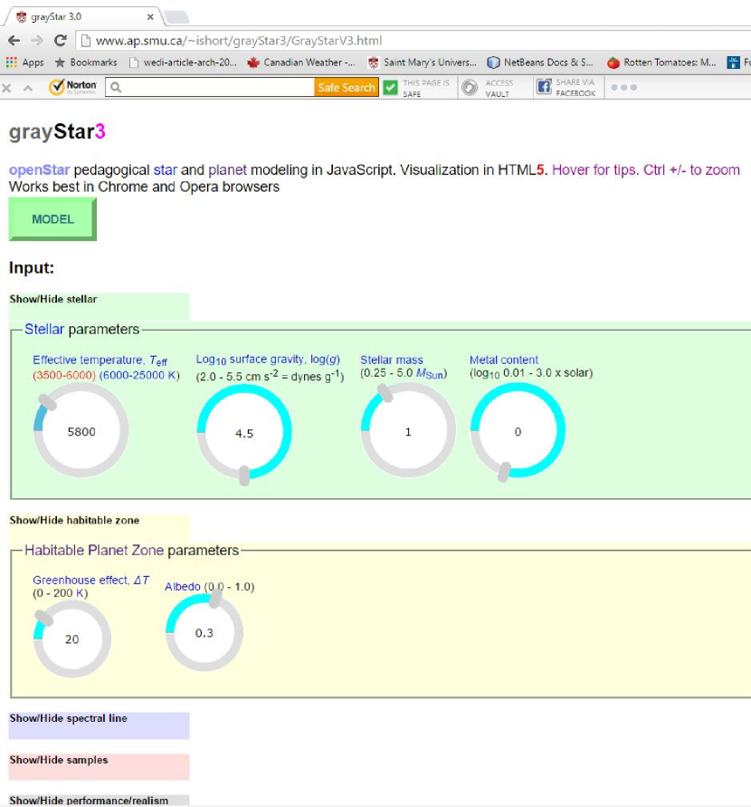
Figure 1: A screen-shot of the gS3 input panel in the simple, default mode. The basic stellar parameters (effective (“surface”) temperature, $T_{\rm eff}$, logarithmic surface gravity, $\log g$, mass, $M$, and logarithmic metallicity, $[{{\rm M}\over{\rm H}}]$) and the planetary surface parameters (greenhouse effect, $\Delta T$, and albedo, $A$) may be controlled with either intuitive and inviting circular sliders, or, for greater precision, by editing a slider’s central text box.

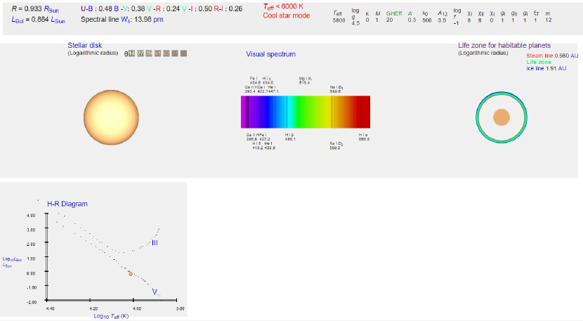
Figure 2: A screen-shot of the gS3 output panel in the simple, default mode. From left-to-right and top-to-bottom the view shows the limb-darkened and -reddened stellar disk, a direct image of the visible flux spectrum with 14 important MK classification or Fraunhofer spectral lines included, the circumstellar habitable zone (CHZ) with steam and ice lines, and an Hertzsprung-Russell (HR) diagram showing the position of the modeled star.

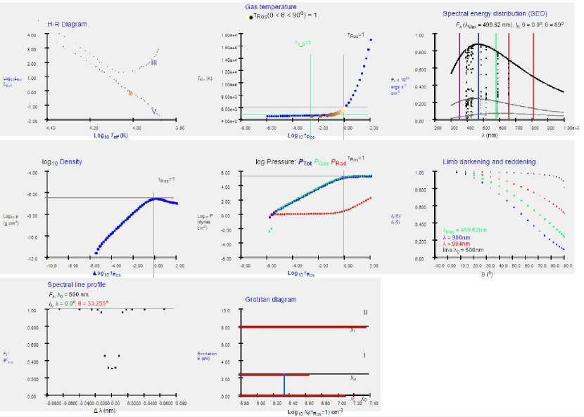
Figure 3: A screen-shot of the gS3 output panel with all the additional advanced panels displayed (along with the HR diagram again). The view shows a group of three plots displaying the vertical atmospheric structure ($T_{\rm kin}(\tau)$, $P_{\rm Tot}(\tau)$, $P_{\rm Gas}(\tau)$, $P_{\rm Rad}(\tau)$, and $\rho(\tau)$ - upper left block), a group of two plots showing the emergent surface radiation field (limb darkening curves, $I_{\lambda}(\lambda,\theta)$, and the SED, $F_{\lambda}(\lambda)$ - right column), and a group of two plots showing the representative high resolution spectral line and the associated Grotrian diagram showing the corresponding $b-b$ transition and associated atomic $E$-levels with level populations - bottom row.

3 User interface

S14a contains a detailed description of the input fields and output panels of the GS2 UI, and gS3 retains the same overall organization. I focus on those new aspects that contrast with GS2.

3.1 Simple mode

When the user first loads the application, it now appears in its simplest display mode by default, presenting the user with only the four inputs controlling the basic parameters of the star to be modeled (effective temperature ($T_{\rm eff}$), surface gravity ($\log g$), mass ($M$), and metallicity ($[{{\rm M}\over{\rm H}}]$), defaulted to their solar values, and two additional parameters for the surface conditions of a planet orbiting the star (greenhouse effect ($\Delta T$) and albedo ($A$)), defaulted to the values for Earth. The default outputs are limited to a logarithmically scaled rendering of the limb-darkened and -reddened projected stellar disk, a rendering of the direct image of the visual spectrum (380 to 680 nm), the Hertzsprung-Russell diagram (HRD) with a logarithmically scaled and appropriately colored symbol showing the location of the modeled star, and a logarithmically scaled diagram of the circumstellar habitable zone (CHZ) showing the location of the steam and ice lines. Figs. 1 and 2 show the input and output areas, respectively, in this mode.

Because gS3 now computes $I_{\lambda}(\theta)$ at 21 $\theta$ values, there are now 20 annuli composing the image of the projected stellar disk, allowing the limb-darkening and -reddening to appear as a more natural looking continuous radial color and brightness gradient. Because gS3 now includes the opacity of fourteen important spectral classification and Fraunhofer spectral lines in its computation of the SED, the rendering of the visual spectral image naturally shows the corresponding dark line features with the strength and width appropriate for the model parameters. This rendering of the spectral image effectively has an inverse linear dispersion in units of nm pixel^-1, and trial and error experimentation indicates that at least 200 $\lambda$ values are required in the sampling of the visible SED to resolve these strong lines.

These default inputs and outputs are limited to those that are the most self-explanatory or suggestive, and the inputs are now set by manipulating attractive and intuitive control knobs that are accompanied by a numeric display showing the precise value to which they have been set. If needed, the values of these parameters can also be set precisely by typing into the accompanying numeric display field.

Color management

The rendering of the limb-darkened and -reddened projected disk has been improved. GS2 used a heuristic mapping of the $T_{\rm kin}(\tau_{\theta}=1)$ value along each $I_{\lambda}(\theta)$ beam onto the RGB 24-bit color palette. gS3 produces the rendering more naturally by passing the $I_{\lambda}(\theta)$ distribution at each $\theta$ value through the B, V, and R filters of the Johnson UBVRI photometric filter set (Johnson et al., 1966) to produce band-integrated intensities, $I_{\rm B}$, $I_{\rm V}$, and $I_{\rm R}$, and a total visible intensity, $I_{\rm Tot}=I_{\rm B}+I_{\rm V}+I_{\rm R}$, at each of the 21 $\theta$ values. It then computes the raw ratios $I_{\rm B}/I_{\rm Tot}$, $I_{\rm V}/I_{\rm Tot}$, and $I_{\rm R}/I_{\rm Tot}$ for each $\theta$ value, and normalizes them with the corresponding raw ratios near disk center ($\theta\approx 0$) computed with a gS3 model of Vega’s parameters ($T_{\rm eff}=9550$ K, $logg=3.95$ (Castelli & Kurucz, 1994)). These calibrated $I_{\rm B}/I_{\rm Tot}$, $I_{\rm V}/I_{\rm Tot}$, and $I_{\rm R}/I_{\rm Tot}$ ratios are then converted into the B, G, and R values, respectively, in the 24-bit RGB color palette for rendering the corresponding 20 annuli in the disk image. Computing the 24-bit RGB colors for the rendering of the direct image of the visible spectrum requires a mapping of monochromatic wavelength, $\lambda$, onto the 24-bit RGB palette. This is a very complex problem and gS3 uses a conversion routine from Glynn (2006), ported from C to JavaScript by the author, that performs the conversion piecewise in seven $\lambda$ ranges.

3.2 Advanced modes

The user now must opt in to revealing additional input panels that control more advanced aspects of the modeling, and output panels that display more technical quantities. The more advanced input panels retain the basic numeric input fields as the sole way of specifying the parameter values, as these allow for the precision required in more serious applications.

Line parameters

The panel controlling the parameters affecting the strength and width of the representative high resolution spectral line and the Grotrian diagram of the corresponding model atom has been expanded. In addition to the wavelength ($\lambda$), logarithmic abundance ($A_{\rm 12}$), oscillator strength ($f_{\rm lu}$), excitation potential of the lower $E$-level of the bound-bound ($b-b$) transition ($\chi_{\rm l}$), neutral stage ground state ionization energy ($\chi_{\rm I}$), particle mass ($m$), micro-turbulence ($\xi_{\rm T}$), and Lorentzian collisional broadening enhancement parameter ($\Gamma_{\rm Col}$), there is now also the ionization potential of the singly ionized stage ($\chi_{\rm II}$), and the statistical weights of the lower $E$-level of the bound-bound ($b-b$) transition, and the ground states of the neutral and singly ionized stages, $g_{\rm l}$, $g_{\rm I}$, and $g_{\rm II}$, respectively. The new $\chi_{\rm II}$ and $g_{\rm II}$ parameters are now necessary to model lines arising from the singly ionized stage, such as the important Ca II $H$ and $K$ lines.

Preset samples

The set of included sample stars (stellar parameter presets) has increased from four to seven. In addition to the original standard stars (the Sun (G2 V), Vega (A0 V), Procyon (F5 IV), and Arcturus (K2 III)), there is now Regulus (B8 IV) anchoring the hot end of the sample space, and two late-type dwarfs that are well-known for hosting extra-solar planetary systems, 51 Pegasi (G5 V, near-solar-like) and 61 Cygni A (K5 V). (Additionally, there is now a set of samples for the accompanying planet, but, for now, it has one member - Earth!). The set of sample spectral line (lines parameter presets) has been expanded from the original three to ten lines that are either important MK spectral classification diagnostics or historically important Fraunhofer lines. In addition to the Na I $D_{\rm 1}$ and $D_{\rm 2}$ and Mg I $b_{\rm 1}$ lines, there are now also the Ca II $H$ and $K$ lines (maximally strong at spectral class K0), the Ca I 4227, and Fe I 4045 and 4271 lines, indicative of late-type stars, and the He I 4471 and 4387 lines indicative of early B stars. These lines, along with the first four members of the H I Balmer series, are the same ones that are included in the rendering of the direct image of the visual spectrum that is now included among the outputs.

Modeling realism and performance

There is a new panel that allows a more advanced user to opt in to including the additional physics discussed in Section 2 to produce a more realistic result, albeit at the cost of execution time. Each of these optional modules addresses an important topic that might arise in a more advanced undergraduate, or introductory graduate level, course, such as thermal equilibrium and temperature corrections, photon scattering in spectral line formation, and convection. This panel also contains the control that allows the user to put gS3 into spectral line modeling mode. In this mode the code does not re-compute the vertical atmospheric structure or overall radiation field, but retrieves them from memory and only recomputes the spectral line. This mode decreases execution time on lower power devices, and is well suited for studies of the simple curve of growth (COG) of a spectral line, which requires many line profile calculations at fixed stellar parameters.

Output panels

Control over which outputs are displayed has now been simplified. The user can turn on three conceptual groups of advanced panels: Plots showing the vertical structure of the atmosphere ($T_{\rm kin}(\tau)$, $P_{\rm Tot}(\tau)$, $P_{\rm Gas}(\tau)$, $P_{\rm Rad}(\tau)$, and $\rho(\tau)$); Plots showing the overall distribution of the surface intensity ($I_{\lambda}(\lambda,\theta)$) and flux ($F_{\lambda}(\lambda)$) fields; And plots showing the representative high resolution spectral line and the Grotrian diagram showing the corresponding $b-b$ transition and associated atomic $E$-levels with level populations (occupation numbers) displayed. The plotting procedures have been greatly improved so that $x-$ and $y-$ axes are now graduated with tick marks at canonical values (ie. with mantissae that are whole number multiples of one, two, or five). As a result, gS3 is effectively a public domain library of general plotting and graphics procedures, such as the XAxis() and YAxis() functions that automatically convert arbitrary data vectors into axes scaled and graduated in device coordinates, and the XBar() and YBar() functions, that can be extracted and recycled in other projects that require JavaScript and HTML plotting. Fig. 3 shows the output panel in advanced mode.

4 Education and public outreach

4.0.1 Education

In a university course beyond first year in observational stellar astronomy, or in stellar astrophysics, or even, in its simplest display mode, in a first year course for physics and astronomy majors, gS3 provides the instructor with the means to perform numerical experiments in class to demonstrate important points and trends. Physics education research (PER) has established the efficacy of demonstration-centered methodological pedagogies in which students discuss and make predictions, or cast a vote among multiple choice predictions, thus becoming invested, before the experiment is run (see Knight (2002), Mazur (1996)). Because gS3 is general, and responsive, the instructor can also easily perform ad hoc experiments that were not planned in response to unanticipated questions that arise in class. The gS3 graphical output area contains additional markers that help demonstrate the crucially important connection between the vertical $T_{\rm kin}(\tau)$ atmospheric structure, and observables such as the limb-darkening ($I_{\lambda}(\theta)$) and high resolution line profile (ie. the LTE Eddington-Barbier relation).

Students beyond first year can be assigned lab-style homework assignments, or major term projects, that are based on following an experimental procedure with gS3. gS3 displays a variety of alpha-numeric quantitative observables and other outputs ($R$, bolometric luminosity, $L_{\rm bol}$, the five photometric indices of Section 2.9, and $W_{\lambda}$) that can be reliably logged in a spreadsheet by ’copy-and-pasting’ (see S14a) to construct data tables and plots. gS3 is especially well suited for labs in which students study the variation of the $W_{\lambda}$ value of the high resolution spectral line with a variety of stellar and line formation input parameters to explore, eg. the curve-of-growth (COG) of a spectral line, or the effect of excitation and ionization equilibrium on lines of different excitation potential arising from the first and second ionization stages (I and II) and the physical basis of MK spectral classification. One must take care in the latter case to work around the current (as of this writing) discontinuous drop in the background $\kappa$ value around a $T_{\rm eff}$ value of 6100 K (see Section 2) by having students separately investigate trends among GK stars, and trends among B, A, and F stars.

Advanced:

At the fourth year honors, or introductory graduate level, students might be asked to undertake projects that require modifying, or even developing, the code. gS3 offers a smaller source code volume, and a more accessible code management paradigm, than research-level FORTRAN codes. The multi-gray temperature correction module (see Section 2) is a particularly compelling example: students could be asked to experiment with the number of multi-gray bins, the $\lambda$ break-points, the relative bin-wise gray opacity levels ($\kappa_{\lambda}$) and thermal emission coefficients ($\epsilon_{\lambda}$), and the number of $\Lambda$-iterations, and to study the effect on $T_{\rm kin}(\tau)$ and related observables such as strong line profiles.

High school:

It is important, and in the interest of the higher education astronomy community, to devise ways of reaching out to high school teachers to help them understand how gS3 can be used effectively, in it simplest display mode, in a unit on basic stellar astronomy. This should involve developing lesson plans and homework assignments around gS3, as well as more significant independent projects for especially keen students. The $T_{\rm eff}$-color relation, the $\log g$-radius relation, and the relations between the location of the CHZ and the $T_{\rm eff}$ and $R$ value of the star and the greenhouse effect and albedo of the planet should all be suitable.

4.1 Public outreach

Its worth noting that as a public WWW application, gS3 is discoverable by anyone, including high-school-aged science enthusiasts who may be strong science students. The hope is that gS3, in its simplest display mode, will entice such users to experiment with the inputs and thereby independently re-discover important relations such as the $T_{\rm eff}$-color relation. The links to pedagogical supporting documents provide keen users with a way to verify what they’ve learned by experimentation. Conversely, a user who is uncertain about their understanding of a concept, including somewhat more advanced ideas such as the relation between $T_{\rm eff}$ and the spectral lines that are visible in the direct image of the visible spectrum, can verify their understanding by by performing relevant experiments with gS3. In this way the young user can feel that they own the knowledge in that they acquired it through their own experimentation. The inclusion of the CHZ in gS3 allows a young user to investigate for themselves the implications whenever they encounter news reports of exo-planets that have been discovered around stars with parameters that differ from those of the Sun. The hope is that some will thus be motivated to study astronomy and astrophysics, or at least cognate sciences, at the university level.

5 Open source and public domain

gS3 is a public domain, open source project. From the gS3 WWW site (www.ap.smu.ca/$\sim$ ishort/grayStar3) anyone may download their own local installation. In addition to not relying on a connection to a remote server, the user may then modify and develop their own version. A relatively straightforward and effective modification would be to change all the pedagogical links so that they point to the relevant section of local on-line astrophysics notes. Although it is ready to be used in its current state as a “finished project” for many EPO purposes, it is also very much a work in progress that could benefit from further development. There may be scope to develop the UI to make it more intuitive, welcoming, and pedagogically effective. There is certainly scope to improve the physical modeling (see Section 2), and the opportunities for development will only increase as commonplace computational devices, web browsers, and and JavaScript interpreters become more powerful. For those who wish to co-develop a centrally version controlled version, both the JavaScript+HTML (gS3) and Java+JavaFX (GrayFox3) versions are on GitHub (https://github.com/sevenian3/GrayStar3, and https://github.com/sevenian3/GrayFox3).

For anyone who wants to be involved, including those who are not computational astrophysicists, there is work to be done developing lesson plans, homework and lab assignments, and independent project ideas at both the university and high school level, reaching out to high school teachers to help them understand how gS3 may be used effectively at the high school level, and assessing the pedagogical efficacy of gS3 by surveying students who have taken a course that incorporates gS3 in the lecture, the lab projects, or both.

6 Community

An important part of the openStars initiative and the grayStar project is to foster a vigorous and freewheeling on-line community of users and developers. To get the most out of the application, users should share ideas for, and experiences with, demonstrations, lesson plans, and lab projects that incorporate grayStar, as well as ways of assessing pedagogical efficacy, and the results thereof. Developers, of either the UI or the physics engine, should share development ideas and problems. To this end, there is both a blog (https://www.blogger.com/blogger.g?blogID=8794336840328957655$\#$overview) and a facebook group (https://www.facebook.com/GrayStarModels?ref=hl) for the grayStar project, and anyone interested is encouraged to exploit these forums.

7 Conclusions

gS3 effectively allows any WWW browser running on any of a broad range of devices for which a browser is available to become a virtual, adjustable, observable star. Depending on the complexity of the optional display modes, this allows the stellar astronomy and astrophysics instructor to engage in demonstration-centered classroom pedagogy, and allows anyone interested, including high-school-age science enthusiasts, to explore and discover through playful experimentation.

The openStar project and gS3 in particular serve as a proof-of-concept of a novel approach to pedagogical scientific computer simulation. gS3 demonstrates that JavaScript natively provides for scientific programming of some sophistication, that WWW browser-based JavaScript interpreters can interpret programs that are on the order of $10^{4}$ lines of code quickly enough, and that the executable code they produce is efficient enough to allow applications requiring on the order of $10^{4}$ to $10^{5}$ double-precision floating point operations, to execute in just a few seconds of wall-clock time on even commonplace portable devices. Presumably these performance metrics will improve as commonplace computers become more capacious and as WWW browsers and JavaScript computers become more powerful and versatile.

sS3 is a public domain, open source project that may be taken as either a “finished-enough” product for many pedagogical demonstrations right now, or as a work in progress that could benefit from further development, both of its UI and of the underlying physical modeling (the “physics engine” behind the rendering).

7.1 Philosophical considerations

As university professors in our particular disciplines, it is arguably our fundamental calling to find ways to use our special “powers” to be relevant to the world. In addition to the traditional ways of doing so (teaching University courses, performing and disseminating research, giving public outreach presentations, and, for a few, developing a text book), this may include novel ways that are enabled by new technology, such as that described here.

Any atmospheric and spectrum modeling code is a type of text-book, written in computer code and comment lines, on the hard-won knowledge of atmospheric and spectrum formation physics, and how to computationally model it, that has been accumulated over the decades. In this analogy, if research-level modeling codes are monumental advanced graduate-level texts kept behind locked doors, gS3 is a slimmer undergraduate text on the most basic aspects that is freely available to anyone who is interested. In this way, gS3 diversifies the “habitat” of this hard-won and important area of knowledge.

In contemporary popular and youth culture, an idea seems to be more relevant if one can experience it through a WWW browser (however ironic or unfortunate that statement may be). By making the process of computational modeling, and the inference of physical parameters from computed observables, into a populist, even frivolous, WWW “activity”, the very idea may become, at least unconsciously, normalized in the minds of adolescent science enthusiasts who “play” with gS3 in its simple mode. Hopefully, some of these will tell their parents (who may be business leaders, investment fund managers, lawyers, journalists, legislators, policy advisers, or educators) what they are doing on the Web, especially the CHZ and greenhouse effect aspect, and the idea will become normalized in their minds as well. This normalization, by itself, may be a step in the right direction in helping humanity incorporate the methods and worldview of science more broadly.

With JavaScript, the WWW browser is the computer (albeit a virtual one) that is being programmed, and the underlying physical architecture and the operating system (OS) are irrelevant to the program-management process. The community that motivates the development of Web-programming technology and commonplace computers is huge, exuberant, free-wheeling, motivated by high stakes, and constantly anxious for progress. Assuming that commonplace computers, WWW browsers, and browser-based JavaScript interpreters become increasingly powerful, capacious, and versatile, one can imagine the possibility that research-level scientific modeling codes may some day be ported to JavaScript. This has implications for radical cloud computing and for computational citizen science, where any idle processor in any kind of device that is equipped with a WWW browser, including smart phones and gaming consoles (and maybe some day soon cars and household refrigerators!) can be put to work on part of a large-scale computational project. Even if JavaScript never becomes a high performance computing language, or one that lends itself to parallelization at the algorithm level, any radically platform-independent programming paradigm does lend itself to parallelization at the job control level, particularly for projects that require a large grid of models that can tolerate asynchronous model generation. This sweeping potential of the WWW browser to become more than it seems should be drawn to the attention of the browser development industry so that they can prioritize the relaxation of the restrictions on browser-based client-side scripting.

References

- Castelli & Kurucz (1994) Castelli, F. & Kurucz, R.L., 1994,. Model atmospheres for VEGA, A&A, 281, 817
- Dufay (2012) Dufay, J., 2012, Introduction to Astrophysics, The Stars, Publ: Dover.
- Gray (2005) Gray, D.F., 2005, The Observation and Analysis of Stellar Photospheres, Third Ed., Cambridge University Press
- Glynn (2006) Glynn, E.F., 2006, “efg’s Computer Lab Science and Engineering Spectra Lab Report: Visible Light Spectrum and Hydrogen Emission/Absorption Spectra”, www.efg2.com/Lab/ScienceAndEngineering/Spectra.htm
- Johnson et al. (1966) Johnson, H. L., Mitchell, R. I., Iriarte, B. & Wisniewski, W. Z., 1966, Comm. Lunar Planet. Lab., 4, 99
- Knight (2002) Knight, R.D., 2002, “Five Easy Lessons: Strategies for Successful Physics Teaching”, Addison-Wesley
- Mazur (1996) Mazur, E., 1996, “Peer Instruction: A User’s Manual”, Addison-Wesley
- Short (2014a) Short, C.I., 2014a, JRASC, 108, 230, arXiv:1409.1891, S14a
- Short (2014b) Short, C.I., 2014b, arXiv:1409.1893, S14b