Resurrecting the minimal renormalizable
supersymmetric SU(5) model

Abstract

It is a well-known fact that the minimal renormalizable supersymmetric SU(5) model is ruled out assuming superpartner masses of the order of a few TeV. Giving up this constraint and assuming only SU(5) boundary conditions for the soft terms, we find that the model is still alive. The viable region of the parameter space typically features superpartner masses of order $10^{2}$ to $10^{4}\,\mathrm{TeV}$, with $\tan\beta$ values between $2$ and $5$, but lighter spectra with single states around $10$ TeV are also possible. The main constraints come from proton decay, the Higgs mass, the requirement of the SU(5) spectrum being reasonably below the Planck scale, and the lifetime of the universe. A generic feature of the model is metastability of the electroweak vacuum. In the absence of a suitable dark matter particle in the neutralino sector, a light (order GeV or smaller) gravitino is a natural candidate.

1 Introduction

The minimal renormalizable supersymmetric SU(5) model [1], with just 3 pairs of $\bf 10\oplus\bar{5}$ fermion representations and an adjoint $\bf 24$ plus a $\bf 5\oplus\bar{5}$ pair in the Higgs sector, is the simplest supersymmetric Grand Unified extension of the Standard Model. It is therefore particularly important to test this model in detail, and possibly to rule it out. Although the choice of the gauge group, supersymmetry and minimality do not need a special motivation, it is more difficult to justify the absence of non-renormalizable terms in the superpotential. Experimental evidence tells us that some of these terms must be strongly suppressed. For instance, the superpotential operators $Q_{1}Q_{1}Q_{2}L_{k}/M_{Planck}$ ($k=1,2,3$) induce proton decay at an unacceptable rate unless they come with coefficients smaller than about $10^{-7}$. Their smallness will lead us to assume in this paper that for some (to us unknown) reason all non-renormalizable operators can be neglected, and to adopt the minimal renormalizable supersymmetric SU(5) model as a benchmark.

It has been shown long ago [7] that the region of the parameter space of the minimal renormalizable supersymmetric SU(5) model corresponding to TeV-scale soft terms is excluded. The reason put forward was the incompatibility between the colour triplet mass constraints associated with gauge coupling unification on the one hand, and with proton decay on the other hand. This conclusion relies however on the assumption of a relatively light superpartner spectrum (although masses as large as $10\,\mathrm{TeV}$ for the first two generations of sfermions were considered in Ref. [7]). The purpose of this paper is to ascertain whether it can be extended to the region of larger superpartner masses.

In order to answer this question, several constraints have to be imposed on the model: precise gauge coupling unification, correct predictions for charged fermion masses, the Higgs mass constraint, the experimental bound on the proton lifetime, and finally the experimental bounds from flavour physics and from direct searches for supersymmetric particles. We also require perturbativity of the model. The observed down-type quark and charged lepton masses are accounted for by generation-dependent supersymmetric threshold corrections with large A-terms [8, 9, 10, 11, 12, 13, 14], which in turn are bounded by considerations related to the stability of the electroweak vacuum [15, 16, 17]. The soft supersymmetry breaking terms are required to respect SU(5) invariance but are not assumed to be flavour universal as in the so-called mSUGRA model (as a matter of fact, generation-dependent A-terms are needed to correct the SU(5) fermion mass relations). To avoid potentially dangerous flavour effects, we will therefore take the GUT-scale sfermion soft terms to be aligned with fermion masses [18]. Neutrino masses can be generated either through bilinear R-parity violation [19, 22, 23, 24] or by adding right-handed neutrinos to the model in order to implement the seesaw mechanism [25]. Finally, if the neutralino sector does not contain a suitable candidate for dark matter (either because the lightest neutralino is not the lightest supersymmetric particle, or because it is too heavy), this role may be played by the gravitino.

Not surprisingly, the main constraint on the superpartner mass scale comes from proton decay, which pushes the spectrum above the $10\,\mathrm{TeV}$ scale (the conflict between the proton decay and unification constraints pointed out in Ref. [7] is resolved by relaxing the upper bound on the superpartner masses). Perturbativity imposes an upper bound on the coloured triplet mass, which translates into an upper limit on superpartner masses once gauge coupling unification is imposed. The observed Higgs mass, together with vacuum metastability constraints associated with the stop A-term, also excludes large portions of the parameter space. A priori, there is no guarantee that the minimal renormalizable supersymmetric SU(5) model will survive all these constraints, even if very large values of the soft terms are allowed.

To give an idea of how the parameter space is restricted by the various phenomenological requirements, we show in Fig. 1 the approximate constraints in the ($\tan\beta$, $m_{susy}$) plane obtained by making several simplifying assumptions. Namely, all sfermion masses are taken to be equal to $m_{susy}$ at the low scale, as well as the $\mu$ parameter and $m_{H_{u}}$ ($m^{2}_{H_{u}}>0$ is assumed, and $m^{2}_{H_{d}}$ and the $B$ parameter are computed from the electroweak symmetry breaking conditions), while the gaugino masses assume a common value $M_{1/2}=m_{susy}$ at the GUT scale and are split by renormalization group running. Obviously, these inputs are not consistent with SU(5) symmetry of the soft terms at the GUT scale, but they make it possible to show several constraints in a single plot. Imposing SU(5) boundary conditions will significantly affect quantities such as the heavy colour triplet mass and more crucially the proton lifetime, making the investigation of the parameter space of the minimal renormalizable supersymmetric SU(5) model more involved than suggested by Fig. 1. As we are going to see, phenomenologically viable points typically feature superpartners in the ${\cal O}(10^{2}-10^{4})\,\mathrm{TeV}$ range, with values of $\tan\beta$ between $2$ and $5$, but lighter spectra with supersymmetric particles as light as a few $10\,\mathrm{TeV}$ can also be found.

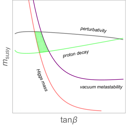
Figure 1: Approximate constraints on the minimal renormalizable supersymmetric SU(5) model in the $(\tan\beta,m_{susy})$ plane. The region to the left of the red curve is excluded by the measured Higgs boson mass, while the area to the right of the purple curve is excluded by vacuum stability considerations (namely, the value of the stop A-term needed to reproduce the observed Higgs boson mass would render the electroweak vacuum unstable with a lifetime shorter than the age of the universe). The experimental lower bound on the proton lifetime is satisfied above the green line, and the perturbativity constraint $m_{T}<M_{Planck}/10$, where $m_{T}$ is the colour triplet mass, is satisfied below the black line. The green area is consistent with all four constraints. In this plot, the sfermion masses, the $\mu$ parameter and $m_{H_{u}}$ are all equal to $m_{susy}$, as well as the common gaugino mass at the GUT scale. Since these values are not consistent with SU(5) boundary conditions, the figure should be considered as illustrative only.

In the process we have generalized the procedure of Refs. [26, 27] for deriving approximate semi-analytic solutions to the one-loop renormalization group equations (RGEs) for the MSSM soft terms. In this way we are able to write the low-energy soft terms as linear or quadratic functions of the initial (GUT-scale) parameters, making it possible to explore the parameter space without having to solve the RGEs for each point. In practice, one just needs to solve numerically the RGEs for gauge and Yukawa couplings for each choice of $\tan{\beta}$ and $m_{susy}$, the matching scale between the SM and the MSSM. The low-energy soft terms and their dependence on the other model parameters are then simply given by linear and quadratic algebraic equations.

The paper is organized as follows. Section 2 introduces the minimal renormalizable supersymmetric SU(5) model. In Section 3, the running of the model parameters is discussed, and the semi-analytical procedure used to solve the renormalization group equations (RGEs) is presented in Section 4 (more details can be found in Appendix A). Proton decay and the constraints associated with the metastability of the electroweak vacuum are addressed in Sections 5 and 6, respectively, with technical details relegated to Appendices B, C and D. Finally, we present our results in Section 7.

2 The minimal renormalizable supersymmetric SU(5) model

In this section, we briefly describe the minimal renormalizable supersymmetric SU(5) model [1] and present our notations. The Higgs sector includes the adjoint $24_{H}$, which spontaneously breaks the SU(5) gauge group to SU(3)$\times$SU(2)$\times$U(1), and a fundamental and anti-fundamental representations $5_{H}$ and $\bar{5}_{H}$ containing the two light Higgs doublets responsible for electroweak symmetry breaking. The $5_{H}\oplus\bar{5}_{H}$ Higgs fields also includes a heavy pair of colour triplet and antitriplet that mediate proton decay through $d=5$ operators. All matter fields belong to $10_{i}$ and $\bar{5}_{i}$ representations (leaving aside right-handed neutrinos in the singlet representation that may also be present), where $i=1,2,3$ is the generation index.

In order to connect the minimal renormalizable supersymmetric SU(5) model with experimental data, one has to deal with three different theories: SU(5) above the unification scale $M_{GUT}$, the Minimal Supersymmetric Standard Model (MSSM) between $M_{GUT}$ and the supersymmetry scale $m_{susy}$, and the Standard Model (SM) between $m_{susy}$ and the weak scale $m_{Z}$. Since the heavy GUT states (resp. the superpartners) are not degenerate in mass, the matching between the SU(5) theory and the MSSM at $M_{GUT}$ (resp. between the MSSM and the SM at $m_{susy}$) will involve threshold corrections.

In the next subsections we give the relevant parts of the corresponding Lagrangians (i.e. the Higgs and Yukawa sectors and the soft supersymmetry breaking terms, which determine the superpartner spectrum) and we specify our notations and assumptions.

2.1 The SU(5) model

The superpotential of the minimal renormalizable supersymmetric SU(5) model is determined by its field content, gauge invariance and renormalizability. It can be divided into two parts describing the Higgs and Yukawa sectors, respectively:

$$W_{H} \ =\ \frac{\mu_{5}}{2}\operatorname{Tr}24_{H}^{2}+\,\frac{\lambda_{5}}{3}\operatorname{Tr}24_{H}^{3}+\bar{5}_{H}\left(\mu_{H}+\eta_{H}\,24_{H}\right)5_{H}\,,$$ (2.1)

$$W_{Y} \ =\ \frac{1}{4}\,\Lambda^{10}_{ij}\,10_{i}10_{j}5_{H}-\sqrt{2}\,\Lambda^{\bar{5}}_{ij}\,\bar{5}_{i}10_{j}\bar{5}_{H}\,,$$ (2.2)

in which we have omitted terms involving right-handed neutrinos as well as R-parity violating couplings that may be present, depending on how neutrino masses are generated. After having solved the equations of motion for the $24_{H}$ in the SM singlet direction:

$$\langle 24_{H}\rangle\,=\,\sigma_{0}\,\mbox{Diag}(2,2,2,-3,-3)\;,\qquad\sigma_{0}\,=\,\mu_{5}/\lambda_{5}\,,$$ (2.3)

and performed the fine-tuning needed to achieve doublet-triplet splitting in the Higgs sector, one can write down the masses of the heavy states in terms of the SU(5) superpotential parameters:

$$m_{V}=5g_{\scriptscriptstyle GUT}\sigma_{0}\,,\ \ \quad m_{T}=5\eta_{H}\sigma_{0}\,,\ \ \quad m_{8}=-m_{3}=-5m_{1}=5\lambda_{5}\sigma_{0}\,,$$ (2.4)

where $m_{V}$ is the mass of the SU(5) gauge bosons in the representations $(3,2)_{-5/3}\oplus(\bar{3},\bar{2})_{+5/3}$ of the SM gauge group; $m_{T}$ is the mass of the colour triplet and antitriplet pair $(T,\bar{T})$ contained in $5_{H}\oplus\bar{5}_{H}$; and $m_{1}$, $m_{3}$ and $m_{8}$ are the masses of the SM singlet, SU(2) triplet and SU(3) octet components of $24_{H}$, respectively. Demanding that the superpotential couplings $\lambda_{5}$ and $\eta_{H}$ be in the perturbative regime and taking into account the fact that the unified gauge coupling $g_{\scriptscriptstyle GUT}$ is of order $1$, one obtains the following constraint:

$$m_{T},\,m_{8},\,m_{3} \ \mathrel{\hbox to0.0pt{\lower 4.0pt\hbox{\hskip 1.0pt$\sim$}\hss}\raise 1.0pt\hbox{$<$}}\ m_{V}\,.$$ (2.5)

We also assume that supersymmetry breaking is coming from above the GUT scale, as for example in supergravity. In practice this means that the soft terms should be SU(5) symmetric at the GUT scale:

$$-{\cal L}_{soft} = (m^{2}_{10})_{ij}\,\tilde{10}^{\dagger}_{i}\tilde{10}_{j}+(m^{2}_{\bar{5}})_{ij}\,\tilde{\bar{5}}^{\dagger}_{i}\tilde{\bar{5}}_{j}+\left(\frac{1}{2}\,A^{10}_{ij}\,\tilde{10}_{i}\tilde{10}_{j}5_{H}-A^{\bar{5}}_{ij}\,\tilde{\bar{5}}_{i}\tilde{10}_{j}\bar{5}_{H}+\mbox{h.c.}\right)$$ (2.6)

$$+\ m_{5_{H}}^{2}\,5^{\dagger}_{H}5_{H}+m_{\bar{5}_{H}}^{2}\,\bar{5}^{\dagger}_{H}\bar{5}_{H}+\left(B_{5}\,5_{H}\bar{5}_{H}+\mbox{h.c.}\right)+\frac{1}{2}\,M_{1/2}\,\bar{\lambda}^{a}\lambda^{a}.$$

We will consider the possibility of generation-dependent soft terms (as explained in the introduction, generation-dependent A-terms are needed to correct the SU(5) fermion mass relations), but in order to comply with the strong constraints coming from flavour physics we must ensure that they do not induce large flavour-violating effects. To this end, we assume that the soft sfermion mass matrices are diagonal in the basis in which the Yukawa couplings $\Lambda^{\bar{5}}$ are diagonal, and that the A-term matrices are diagonal in the corresponding fermion mass eigenstate basis:

$$(m^{2}_{10})_{ij}=m^{2}_{10_{i}}\delta_{ij}\,,\ \ (m^{2}_{\bar{5}})_{ij}=m^{2}_{\bar{5}_{i}}\delta_{ij}\,,\ \ A^{\bar{5}}_{ij}=A^{\bar{5}}_{i}\delta_{ij} \mbox{in the basis}\ \Lambda^{\bar{5}}_{ij}=\Lambda^{\bar{5}}_{i}\delta_{ij}\,,\hskip 28.45274pt$$ (2.7)

$$A^{10}_{ij}=A^{10}_{i}\delta_{ij} \mbox{in the basis}\ \Lambda^{10}_{ij}=\Lambda^{10}_{i}\delta_{ij}\,,$$ (2.8)

so that all flavour violation at the GUT scale is concentrated in the up squark sector and controlled by the CKM angles, yielding an effective alignment of sfermion soft terms with fermion masses [18]. In addition, we assume that the soft masses of the first two generations of sfermions are degenerate:

$$m^{2}_{10_{1}}\,=\,m^{2}_{10_{2}}\,,\quad m^{2}_{\bar{5}_{1}}\,=\,m^{2}_{\bar{5}_{2}}\,.$$ (2.9)

Finally, we will take $M_{1/2}$ and the A-terms (as well as the $\mu$ parameter $\mu\equiv\mu_{H}-3\eta_{H}\sigma_{0}$) to be real. This may be more than what we need to evade flavour and CP constraints from low-energy experiments, especially in view of the fact that the superpartner spectrum is heavy, but this choice also helps reducing the number of parameters. In our subsequent exploration of the parameter space of the minimal renormalizable supersymmetric SU(5) model we shall completely neglect flavour violation in the sfermion sector, including the small amount of flavour violation that is generated from the running of the soft terms.

2.2 MSSM

Below the scale $M_{GUT}$, the relevant theory is the MSSM, with superpotential

$$W_{MSSM} \ =\ \Lambda_{ij}^{U}\,U_{i}^{c}Q_{j}H_{u}\,-\,\Lambda_{ij}^{D}\,D_{i}^{c}Q_{j}H_{d}\,-\,\Lambda_{ij}^{E}\,E_{i}^{c}L_{j}H_{d}\,+\,\mu\,H_{u}H_{d}\,,$$ (2.10)

and soft supersymmetry breaking terms

$$-\,{\cal L}_{soft} = (m^{2}_{\tilde{Q}})_{ij}\,{\tilde{q}}^{\dagger}_{i}{\tilde{q}}_{j}+(m^{2}_{\tilde{u}^{c}})_{ij}\,{\tilde{u}}^{c}_{i}{\tilde{u}}^{c\dagger}_{j}+(m^{2}_{\tilde{e}^{c}})_{ij}\,{\tilde{e}}^{c}_{i}{\tilde{e}}^{c\dagger}_{j}+(m^{2}_{\tilde{L}})_{ij}\,{\tilde{l}}^{\dagger}_{i}{\tilde{l}}_{j}+(m^{2}_{\tilde{d}^{c}})_{ij}\,{\tilde{d}}^{c}_{i}{\tilde{d}}^{c\dagger}_{j}$$ (2.11)

$$+\left(A^{U}_{ij}\,{\tilde{u}^{c}}_{i}{\tilde{q}}_{j}h_{u}-A^{D}_{ij}\,{\tilde{d}^{c}}_{i}{\tilde{q}}_{j}h_{d}-A^{E}_{ij}\,{\tilde{e}}^{c}_{i}{\tilde{l}}_{j}h_{d}+\mbox{h.c.}\right)$$

$$+\ m_{H_{u}}^{2}h_{u}^{\dagger}h_{u}+m_{H_{d}}^{2}h_{d}^{\dagger}h_{d}+\left(B\,h_{u}h_{d}+\mbox{h.c.}\right)$$

$$+\ \frac{1}{2}M_{1}\,\bar{\tilde{B}}{\tilde{B}}+\frac{1}{2}M_{2}\,\bar{\tilde{W}}^{i}{\tilde{W}}^{i}+\frac{1}{2}M_{3}\,\bar{\tilde{g}}^{a}{\tilde{g}}^{a},$$

where the contraction of $SU(2)_{L}$ indices is understood (for instance, $H_{u}H_{d}$ stands for $\epsilon_{ij}H^{i}_{u}H^{j}_{d}=H^{+}_{u}H^{-}_{d}-H^{0}_{u}H^{0}_{d}$, where $i,j=1,2$ are $SU(2)_{L}$ indices and $\epsilon_{ij}$ is the totally antisymmetric tensor with $\epsilon_{12}=+1$). Due to the boundary conditions (2.7) and (2.8), and to the fact that we are neglecting the effects of the CKM matrix in the running, the sfermion soft terms keep a diagonal form all the way down to low energies.

2.3 Standard Model

Below the matching scale

$$m_{susy} \,\equiv\,\sqrt{m_{\tilde{t}_{1}}(m_{susy})\,m_{\tilde{t}_{2}}(m_{susy})}\,\simeq\,\sqrt{m_{\tilde{Q}_{3}}(m_{susy})\,m_{\tilde{u}^{c}_{3}}(m_{susy})}$$ (2.12)

(where the last approximation is valid as long as the mixing in the stop sector is small, i.e. $m_{t}X_{t}\ll m^{2}_{\tilde{Q}_{3}},m^{2}_{\tilde{u}^{c}_{3}}$), the relevant theory is the Standard Model. The Higgs potential is given by (with the SM Higgs doublet given by $h=\sqrt{2}\left(\cos\beta\,h_{d}+\sin\beta\,i\sigma^{2}h^{*}_{u}\right)$ in the decoupling limit):

$$V_{SM} =-\,m_{h}^{2}\,h^{\dagger}h+\frac{\lambda}{2}\left(h^{\dagger}h\right)^{2},$$ (2.13)

while the Yukawa Lagrangian is

$${\cal L}_{Yukawa}=-H_{ij}^{U}\,\bar{u}_{Ri}\tilde{h}^{\dagger}q_{j}-H_{ij}^{D}\,\bar{d}_{Ri}h^{\dagger}q_{j}-H_{ij}^{E}\,\bar{e}_{Ri}h^{\dagger}l_{j}+\mbox{h.c.}\,,$$ (2.14)

where $\tilde{h}\equiv i\sigma^{2}h^{*}$.

3 Renormalization group equations

In this section, we collect the SM and MSSM renormalization group equations (RGEs) and various expressions used in our analysis (from boundary to matching conditions). We use the SM RGEs [28] between $m_{Z}$ and $m_{susy}$, and the MSSM RGEs [29] between $m_{susy}$ and $M_{GUT}$. The gauge and Yukawa couplings, as well as the Higgs quartic coupling are evolved with the 2-loop RGEs, with the 1-loop threshold corrections accounting for the splitting of superpartner masses added at the scale $m_{susy}$. All soft parameters (A-terms, gaugino masses and soft scalar masses) are run at 1 loop.

3.1 Gauge couplings

The 2-loop RGEs for the gauge couplings $g_{i}$ ($i=1,2,3$ for the gauge groups $U(1)_{Y}$, $SU(2)_{L}$ and $SU(3)_{C}$, respectively, with $g_{1}=\sqrt{5/3}\,g^{\prime}$) read:

$$\frac{d}{dt}g_{i} \ =\ \frac{g_{i}^{3}}{(4\pi)^{2}}b_{i}\,+\,\frac{g_{i}^{3}}{(4\pi)^{4}}\left(\,\sum_{j=1}^{3}B_{ij}\,g_{j}^{2}-\!\sum_{\alpha=u,d,e}\!\!C_{i\alpha}\operatorname{Tr}(\Lambda_{\alpha}^{\dagger}\Lambda_{\alpha})\right),$$ (3.1)

where $t\equiv\ln(m/m_{0})$, $m$ being the renormalization group scale, and the $\beta$-function coefficients below and above $m_{susy}$ are given by:

$$b_{i}^{SM} =(41/10,-19/6,-7)\,, \,\,b_{i}^{MSSM}=(33/5,1,-3)\,,$$ (3.2)

$$B_{ij}^{SM} =\left[\begin{array}[]{ccc}199/50&27/10&44/5\\ 9/10&35/6&12\\ 11/10&9/2&-26\end{array}\right]\,, B_{ij}^{MSSM}=\left[\begin{array}[]{ccc}199/25&27/5&88/5\\ 9/5&25&24\\ 11/5&9&14\end{array}\right]\,,$$ (3.9)

$$C_{i\alpha}^{SM} =\left[\begin{array}[]{ccc}17/10&1/2&3/2\\ 3/2&3/2&1/2\\ 2&2&0\end{array}\right]\,, C_{i\alpha}^{MSSM}=\left[\begin{array}[]{ccc}26/5&14/5&18/5\\ 6&6&2\\ 4&4&0\end{array}\right].$$ (3.16)

In the last term of Eq. (3.1), the MSSM Yukawa couplings $\Lambda_{\alpha}$ should be replaced with the SM ones ($H_{\alpha}$) below $m_{susy}$.

At $m_{susy}$, the running gauge couplings should be converted from the $\overline{\textrm{MS}}$ scheme to the $\overline{\textrm{DR}}$ scheme, in which the MSSM RGEs are written:

$$\alpha_{1}^{-1}(m_{susy}+\epsilon) \,=\,\alpha_{1}^{-1}(m_{susy}-\epsilon)\,,$$ (3.17)

$$\alpha_{2}^{-1}(m_{susy}+\epsilon) \,=\,\alpha_{2}^{-1}(m_{susy}-\epsilon)-\frac{1}{6\pi}\,,$$ (3.18)

$$\alpha_{3}^{-1}(m_{susy}+\epsilon) \,=\,\alpha_{3}^{-1}(m_{susy}-\epsilon)-\frac{1}{4\pi}\,,$$ (3.19)

where $\alpha_{i}\equiv g_{i}^{2}/(4\pi)$ and $\epsilon\to 0^{+}$.

3.1.1 Threshold corrections to gauge couplings

Imposing gauge coupling unification at the GUT scale:

$$\alpha_{1}(M_{GUT})\ =\ \alpha_{2}(M_{GUT})\ =\ \alpha_{3}(M_{GUT}) \ \equiv\ \alpha_{GUT}$$ (3.20)

implies certain relations among the masses of the various thresholds (supersymmetric partners of the SM fields and heavy GUT fields). Adding 1-loop threshold corrections [30, 31, 32, 33, 34] to the running gauge couplings evolved with the 2-loop MSSM RGEs between the scales $m_{susy}$ and $M_{GUT}$ yields the following relations ($i=1,2,3$):

$$\alpha_{GUT}^{-1} \ =\overbrace{{}\bar{\alpha}_{i}^{-1}(M_{GUT})}^{\textrm{2-loop single-scale MSSM}}-\overbrace{\frac{1}{2\pi}\ \sum_{n}\Delta b_{i}^{(n)}\ln\frac{m_{susy}}{m_{n}}}^{\textrm{1-loop low-energy threshold corrections}}$$

$$\qquad-\underbrace{\frac{1}{2\pi}\left[\Delta b_{i}^{V}\ln\frac{M_{GUT}}{m_{V}}+\Delta b_{i}^{8}\ln\frac{M_{GUT}}{m_{8}}+\Delta b_{i}^{3}\ln\frac{M_{GUT}}{m_{3}}+\Delta b_{i}^{T}\ln\frac{M_{GUT}}{m_{T}}\right]}_{\textrm{1-loop high-energy threshold corrections}}\ ,$$ (3.21)

where the ${}\bar{\alpha}_{i}$ denote the values of the gauge couplings obtained by solving numerically the 2-loop MSSM RGEs with all superpartner masses at the scale $m_{susy}$, and $n$ runs over the superpartners. Their contributions $\Delta b_{i}^{(n)}$ to the $\beta$-function coefficients are given by:

$$\begin{array}[]{rclrcl}\Delta b_{i}^{\tilde{Q}_{i}}&=&(1/30,1/2,1/3)\,,&\Delta b_{i}^{\tilde{h}}&=&(2/5,2/3,0)\,,\\ \Delta b_{i}^{\tilde{u}_{i}}&=&(4/15,0,1/6)\,,&\Delta b_{i}^{A}&=&(1/10,1/6,0)\,,\\ \Delta b_{i}^{\tilde{d}_{i}}&=&(1/15,0,1/6)\,,&\Delta b_{i}^{\tilde{b}}&=&(0,0,0)\,,\\ \Delta b_{i}^{\tilde{L}_{i}}&=&(1/10,1/6,0)\,,&\Delta b_{i}^{\tilde{w}}&=&(0,4/3,0)\,,\\ \Delta b_{i}^{\tilde{e}_{i}}&=&(1/5,0,0)\,,&\Delta b_{i}^{\tilde{g}}&=&(0,0,2)\,,\end{array}$$ (3.22)

while the contributions of the heavy GUT fields are:

$$\begin{array}[]{rclrcl}\Delta b_{i}^{8}&=&(0,0,3)\,,&\Delta b_{i}^{3}&=&(0,2,0)\,,\\ \Delta b_{i}^{1}&=&(0,0,0)\,,&\Delta b_{i}^{T}&=&(2/5,0,1)\,,\\ \Delta b_{i}^{V}&=&(-10,-6,-4)\,.&&&\end{array}$$ (3.23)

Taking appropriate combinations of the three equations (3.21), one obtains:

$$\frac{m_{T}}{M_{GUT}} \ =\ \exp{\left[\frac{5\pi}{6}\left(-\,{}\bar{\alpha}_{1}^{-1}+3\,{}\bar{\alpha}_{2}^{-1}-2\,{}\bar{\alpha}_{3}^{-1}\right)(M_{GUT})\right]}\left(\frac{m_{3}}{m_{8}}\right)^{5/2}$$

$$\ \times\ \left(\frac{m_{\tilde{w}}}{m_{\tilde{g}}}\right)^{5/3}\prod_{i=1}^{3}\left(\frac{m_{\tilde{Q}_{i}}^{4}}{m_{\tilde{u}^{c}_{i}}^{3}m_{\tilde{e}^{c}_{i}}}\frac{m_{\tilde{L}_{i}}^{2}}{m_{\tilde{d}^{c}_{i}}^{2}}\right)^{1/12}\left(\frac{m_{\tilde{h}}^{4}m_{A}}{m_{susy}^{5}}\right)^{1/6},$$ (3.24)

$$\frac{\left[m_{V}^{2}(m_{3}m_{8})^{1/2}\right]^{1/3}}{M_{GUT}} \ =\ \exp{\left[\frac{\pi}{18}\left(5\,{}\bar{\alpha}_{1}^{-1}-3\,{}\bar{\alpha}_{2}^{-1}-2\,{}\bar{\alpha}_{3}^{-1}\right)(M_{GUT})\right]}$$

$$\ \times\ \left(\frac{m_{susy}^{2}}{m_{\tilde{w}}m_{\tilde{g}}}\right)^{1/9}\prod_{i=1}^{3}\left(\frac{m_{\tilde{u}^{c}_{i}}m_{\tilde{e}^{c}_{i}}}{m_{\tilde{Q}_{i}}^{2}}\right)^{1/36},$$ (3.25)

$$\alpha_{GUT}^{-1} \ =\ \left[\left(-\frac{5}{9}\,{}\bar{\alpha}_{1}^{-1}+\frac{12}{9}\,{}\bar{\alpha}_{2}^{-1}+\frac{2}{9}\,{}\bar{\alpha}_{3}^{-1}\right)(M_{GUT})\right]$$

$$+\ \frac{1}{2\pi}\ln \!\left[\frac{m_{8}^{1/5}m_{3}^{4/5}}{m_{V}}\right]^{10/3}\!+\ \frac{1}{2\pi}\ln\!\left[\frac{m_{\tilde{h}}^{12}m_{A}^{3}m_{\tilde{w}}^{32}m_{\tilde{g}}^{8}}{m_{susy}^{91}}\,\prod_{i=1}^{3}\left(\frac{m_{\tilde{Q}_{i}}^{13}m_{\tilde{L}_{i}}^{3}}{m_{\tilde{u}_{i}^{c}}^{2}m_{\tilde{e}_{i}^{c}}^{2}}\right)\right]^{1/18}.$$ (3.26)

At the 1-loop level, the matching scales $M_{GUT}$ and $m_{susy}$ drop out from Eqs. (3.1.1) and (3.1.1), while only $m_{susy}$ drops out from Eq. (3.1.1). Since $m_{susy}\gg m_{Z}$, one can neglect the mixing between the higgsinos and the electroweak gauginos and identify:

$$m_{\tilde{h}} \ =\ \mu\,,$$ (3.27)

$$m_{A} \ =\ \sqrt{(|\mu|^{2}+m_{H_{d}}^{2}(m_{susy}))(1+1/\tan^{2}{\beta})}$$

$$\ \simeq\ \sqrt{(m_{H_{d}}^{2}(m_{susy})-m_{H_{u}}^{2}(m_{susy}))(\tan^{2}\beta+1)\,/\,(\tan^{2}\beta-1)}\ ,$$ (3.28)

$$m_{\tilde{w}}/m_{\tilde{g}} \ \simeq\ \alpha_{2}(m_{\tilde{g}})/\alpha_{3}(m_{\tilde{g}})\,,$$ (3.29)

where $\tan\beta\equiv\langle h^{0}_{u}\rangle/\langle h^{0}_{d}\rangle$ is the ratio of the two MSSM Higgs doublet vevs, and $\mu$ satisfies the electroweak symmetry breaking (EWSB) condition (again neglecting $m^{2}_{Z}$):

$$|\mu|^{2} \ \simeq\ \frac{m_{H_{d}}^{2}(m_{susy})-m_{H_{u}}^{2}(m_{susy})\tan^{2}{\beta}}{\tan^{2}{\beta}-1}\ .$$ (3.30)

In spite of the initial historical success [35, 36, 37, 38], it is well known that gauge couplings do not unify accurately at the 2-loop level in the MSSM with TeV-scale superpartners. High-energy threshold corrections thus play a crucial role in achieving precise unification [33]. Using Eqs. (3.1.1) and (3.1.1), one can express the combinations of GUT state masses needed for exact 2-loop unification in terms of the superpartner masses [33]. Assuming that all superpartners have masses equal to $m_{susy}$, one obtains for the colour triplet mass and for the combination of heavy gauge boson and adjoint Higgs masses $m_{V}^{2/3}m_{3}^{1/3}$:

$$m_{T} \ \sim\,2\times 10^{15}\,\mathrm{GeV}\,\left(\frac{m_{susy}}{1\,\mathrm{TeV}}\right)^{5/6}\,,$$ (3.31)

$$m_{V}^{2/3}m_{3}^{1/3} \ \sim\,2\times 10^{16}\,\mathrm{GeV}\,\left(\frac{m_{susy}}{1\,\mathrm{TeV}}\right)^{-2/9}\,,$$ (3.32)

where we have used the fact that $m_{3}=m_{8}$ in the minimal renormalizable supersymmetric SU(5) model. For superpartner masses in the TeV range, the colour triplet is far too light and makes the proton decay too fast, which led Ref. [7] to conclude that the minimal renormalizable supersymmetric SU(5) model is excluded (this conclusion has been found to be mitigated at the three-loop level [39] though, and can be avoided for a specific choice of the soft terms [3]).

3.2 Yukawa couplings

For the Yukawa couplings, we use the 2-loop Standard Model RGEs [28] below the scale $m_{susy}$, and the 2-loop MSSM RGEs [29] above it. We neglect all CKM contributions and work with diagonal Yukawa matrices. In the absence of threshold corrections, the matching conditions at $m_{susy}$ are:

$$\lambda_{t,c,u}(m_{susy})\, =\,h_{t,c,u}(m_{susy})/\sin\beta\,,$$ (3.33)

$$\lambda_{b,s,d}(m_{susy})\, =\,h_{b,s,d}(m_{susy})/\cos\beta\,,$$ (3.34)

$$\lambda_{\tau,\mu,e}(m_{susy})\, =\,h_{\tau,\mu,e}(m_{susy})/\cos\beta\,.$$ (3.35)

where the $h$ couplings (resp. the $\lambda$ couplings) are the diagonal entries of the SM Yukawa matrices $H^{U,D,E}$ (resp. of the MSSM Yukawa matrices $\Lambda^{U,D,E}$).

3.2.1 Threshold corrections to Yukawa couplings

At the GUT scale, the SU(5)-invariant boundary conditions apply:

$$\Lambda_{U}(M_{GUT}) \ =\ \Lambda_{U}^{T}(M_{GUT})\,,$$ (3.36)

$$\Lambda_{D}(M_{GUT}) \ =\ \Lambda_{E}^{T}(M_{GUT})\,.$$ (3.37)

Threshold corrections due to the splitting of the heavy GUT state masses slightly modify these relations (see later). After running down to low energy, Eqs. (3.37) lead to predictions for down-type quark and charged lepton masses that are in gross contradiction with the data. Supersymmetric threshold corrections at the scale $m_{susy}$ may cure this problem.

Supersymmetric threshold corrections to light fermion masses

In the following, we will neglect supersymmetric threshold corrections to the leptonic Yukawa couplings, and consider only the corrections to the down-type quark Yukawa couplings, whose dominant contributions are proportional to $\alpha_{3}$ and $\lambda^{2}_{t}$ (see however Ref. [40]). This will allow us to derive the SU(5) Yukawa couplings $\Lambda^{\bar{5}}$ by simply running the charged lepton couplings up to the GUT scale. The leading supersymmetric threshold corrections to down-type quark masses are given by the gluino and higgsino contributions [8, 9, 10, 12, 13, 14] (the latter can safely be neglected for the first two generations):

$$\frac{\Delta m_{d_{i}}}{m_{d_{i}}} \,=\,-\,\frac{2\alpha_{3}}{3\pi}\,m_{\tilde{g}}\,X_{d_{i}}\,I_{3}(m^{2}_{\tilde{g}},m_{\tilde{d}_{L_{i}}}^{2},m_{\tilde{d}_{R_{i}}}^{2})\,+\frac{\lambda_{t}^{2}}{16\pi^{2}}\,\mu\,X_{t}\,\tan\beta\,I_{3}(|\mu|^{2},m_{\tilde{t}_{1}}^{2},m_{\tilde{t}_{2}}^{2})\,\delta_{i3}\,,$$ (3.38)

where

$$X_{t} \,\equiv\,A_{t}/\lambda_{t}-\mu\cot\beta\,,$$ (3.39)

$$X_{d_{i}} \,\equiv\,A_{d_{i}}/\lambda_{d_{i}}-\mu\tan\beta\,,$$ (3.40)

$$X_{e_{i}} \,\equiv\,A_{e_{i}}/\lambda_{e_{i}}-\mu\tan\beta\,,$$ (3.41)

and the loop function $I_{3}$ is defined by:

$$I_{3}(x,y,z) \,=\,-\frac{xy\ln{(x/y)}+yz\ln{(y/z)}+zx\ln{(z/x)}}{(x-y)(y-z)(z-x)}\ ,$$ (3.42)

with the limits

$$I_{3}(x,x,z) \,=\,\frac{1-(z/x)+(z/x)\ln{(z/x)}}{x(1-(z/x))^{2}}\ ,$$ (3.43)

$$I_{3}(x,x,x) \,=\,\frac{1}{2x}\ .$$ (3.44)

The matching is done at the scale $m_{susy}$:

$$m^{\rm SM}_{d_{i}} \,=\,m^{\rm MSSM}_{d_{i}}\left(1+\frac{\Delta m_{d_{i}}}{m_{d_{i}}}\right),$$ (3.45)

where

$$m^{\rm SM}_{d_{i}}\,=\,h_{d_{i}}(m_{susy})\,v\,,\qquad m^{\rm MSSM}_{d_{i}}\,=\,\lambda_{d_{i}}(m_{susy})\,v\cos\beta\,,$$ (3.46)

in which $v=\langle h^{0}\rangle$. As a first approximation, $b\,$–$\,\tau$ Yukawa unification is a relatively successful prediction of SU(5), while the discrepancy between the prediction and the data is much more important for the first two generations. As can be seen from Eq. (3.38), the non-holomorphic ($\propto\mu\tan{\beta}$) contributions to $\Delta m_{d}/m_{d}$ and $\Delta m_{s}/m_{s}$ are the same for equal first two generation squark masses, while the ratios $m_{s}/m_{\mu}$ and $m_{d}/m_{e}$ are widely different. This implies that large A-terms $A_{d}$ and $A_{s}$ are needed to bring these ratios into agreement with experimental data, which in turn makes the electroweak vacuum metastable [12, 13]. This issue will be discussed in Section 6.

High-scale thresholds corrections to $\lambda_{b}$ and $\lambda_{\tau}$

In addition to supersymmetric corrections at the superpartner mass scale, Yukawa couplings are also subject to high-scale threshold corrections due to the heavy GUT states. These may affect in particular bottom-tau Yukawa unification, which as explained before is an important constraint on the model, hence one must take them into account. In practice, all one needs is the difference between $\lambda_{b}(M_{GUT})$ and $\lambda_{\tau}(M_{GUT})$ induced by the GUT-scale threshold corrections. One can check that it is given by:

$$\lambda_{b}(M_{GUT})-\lambda_{\tau}(M_{GUT}) \ =\ \frac{\lambda_{\tau}(M_{GUT})}{(4\pi)^{2}}\left[\lambda^{2}_{t}(M_{GUT})\ln{\frac{M_{GUT}}{m_{T}}}-4\,g_{\scriptscriptstyle GUT}^{2}\,\ln{\frac{M_{GUT}}{m_{V}}}\right]\,.$$ (3.47)

GUT threshold corrections also affect strange quark-mu and down quark-electron Yukawa unification, but the numerical effect is negligible compared with the size of the low-scale (supersymmetric) threshold corrections that are needed to account for the observed masses.

3.3 Higgs quartic coupling

For heavy stop masses, the proper way to compute the lightest supersymmetric Higgs boson mass (for the standard computation, see Refs. [41, 42]) is to consider the effective theory below the scale $m_{susy}$, in which all superpartners and heavy Higgs bosons have been integrated out and the Higgs boson mass is determined from the Higgs quartic coupling $\lambda$, with the value of $\lambda(m_{susy})$ determined by the supersymmetric theory valid above $m_{susy}$. At tree level, the matching condition is $\lambda=\left(3g_{1}^{2}/5+g_{2}^{2}\right)\cos^{2}2\beta/4$, while at the 1-loop level it is given by:

$$\lambda(m_{susy})\ =\ \left(\frac{3}{5}g_{1}^{2}(m_{susy})+g_{2}^{2}(m_{susy})\right)\frac{\cos^{2}{(2\beta)}}{4}\ +\,\Delta\lambda^{reg}\,+\,\Delta\lambda^{\phi}\,+\,\Delta\lambda^{\chi}\,,$$ (3.48)

where the first term on the right-hand side of Eq. (3.48) is the tree-level contribution, $\Delta\lambda^{reg}$ accounts for the conversion of the gauge couplings from the $\overline{\textrm{DR}}$ scheme to the $\overline{\textrm{MS}}$ scheme, and $\Delta\lambda^{\phi}$ and $\Delta\lambda^{\chi}$ are the one-loop threshold corrections due to scalars and electroweak gauginos/higgsinos, respectively, whose expressions can be found in Ref. [43]. The dominant contributions are the ones proportional to $(m_{t}/v)^{4}$ in $\Delta\lambda^{\phi}$, which in the case where all sparticle masses lie close to $m_{susy}$ (and in particular $m_{\tilde{Q}_{3}}\simeq m_{\tilde{u}_{3}}\simeq m_{susy}$) reduce to the leading stop mixing term:

$$\Delta\lambda^{\phi}\,\simeq\,\frac{6h_{t}^{4}}{(4\pi)^{2}}\frac{X_{t}^{2}}{m_{\tilde{t}_{1}}m_{\tilde{t}_{2}}}\left[1-\frac{1}{12}\frac{X_{t}^{2}}{m_{\tilde{t}_{1}}m_{\tilde{t}_{2}}}\right]\,.$$ (3.49)

For large values of $\tan\beta$ and/or large values of $X_{b,\tau}$, one should also include on the RHS of Eq. (3.49) the leading sbottom and stau contributions, which in the limit $m_{\tilde{Q}_{3}}\simeq m_{\tilde{d}_{3}}\simeq m_{\tilde{L}_{3}}\simeq m_{\tilde{e}_{3}}\simeq m_{susy}$ read:

$$\frac{6h_{b}^{4}}{(4\pi)^{2}}\frac{X_{b}^{2}}{m_{\tilde{b}_{1}}m_{\tilde{b}_{2}}}\left[1-\frac{1}{12}\frac{X_{b}^{2}}{m_{\tilde{b}_{1}}m_{\tilde{b}_{2}}}\right]\,+\,\frac{2h_{\tau}^{4}}{(4\pi)^{2}}\frac{X_{\tau}^{2}}{m_{\tilde{\tau}_{1}}m_{\tilde{\tau}_{2}}}\left[1-\frac{1}{12}\frac{X_{\tau}^{2}}{m_{\tilde{\tau}_{1}}m_{\tilde{\tau}_{2}}}\right]\,.$$ (3.50)

Considering only the leading term (3.49), one can see that for each value of $m_{susy}$ and $\tan\beta$ there exist either $4$, $2$ or $0$ different values of $X_{t}$ satisfying the matching condition (3.48). There also exists a lower bound on $m_{susy}$ for each value of $\tan\beta$, reached when $X_{t}$ becomes

$$X_{t}^{max}=\pm\sqrt{6}\,m_{susy}\,,$$ (3.51)

where the stop mixing contribution reaches its maximum [44] (when higher order corrections are included the Higgs mass also depends on the sign of $X_{t}$).

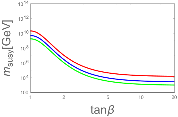
Figure 2: Higgs mass constraint in the ($\tan\beta$, $m_{susy}$) plane for different matching conditions, with all SM parameters set to their central values. The red curve corresponds to the tree-level matching condition and the blue curve to the full 1-loop matching condition (3.48), while for the green curve only the leading 1-loop threshold correction (3.49) was used. Both the blue and green curves assume maximal positive stop mixing ($X_{t}=\sqrt{6}\,m_{susy}$). The superpartner spectrum is chosen as in Fig. 1.

This is illustrated in Fig. 2, in which the lower bound on $m_{susy}$ is represented by the green curve, assuming a superpartner spectrum as in Fig. 1. The comparison with the red curve shows the importance of the 1-loop threshold corrections to the Higgs quartic coupling. Note that the SM parameters were set to their central values in this figure; taking into account the uncertainty on the top quark mass would spread the curves into bands which become very broad at small $\tan\beta$ values. For a discussion on this point, see Ref. [44].

3.4 A-terms

As discussed in the introduction and in Subsection 3.2, we assume the A-term matrices to be diagonal in the corresponding fermion mass eigenstate basis, with generation-dependent entries:

$$A_{U}\, =\,\text{Diag}\,(A_{u},A_{c},A_{t})\,,$$ (3.52)

$$A_{D}\, =\,\text{Diag}\,(A_{d},A_{s},A_{b})\,,$$ (3.53)

$$A_{E}\, =\,\text{Diag}\,(A_{e},A_{\mu},A_{\tau})\,.$$ (3.54)

These matrices are run with the 1-loop MSSM RGEs, with the SU(5) boundary conditions imposed at the GUT scale:

$$A_{U}(M_{GUT})\, =\,A_{U}^{T}(M_{GUT})\,,$$ (3.55)

$$A_{D}(M_{GUT})\, =\,A_{E}^{T}(M_{GUT})\,.$$ (3.56)

3.5 Gaugino masses

For the running of gaugino masses we use the 1-loop RGEs:

$$\frac{d}{dt}M_{i}\, =\,\frac{b_{i}}{2\pi}\alpha_{i}\,M_{i}\,,$$ (3.57)

and impose the SU(5) boundary condition at the GUT scale:

$$M_{1}(M_{GUT})\,=\,M_{2}(M_{GUT})\,=\,M_{3}(M_{GUT}) \,\equiv\,M_{1/2}\,.$$ (3.58)

3.6 Soft scalar masses

We also assume the soft sfermion mass matrices $m^{2}_{\tilde{X}}$ $(X=Q,u^{c},e^{c},L,d^{c})$ to be diagonal with generation-dependent entries:

$$m^{2}_{\tilde{X}}\, =\,\text{Diag}\,(m_{\tilde{X}_{1}}^{2},m_{\tilde{X}_{2}}^{2},m_{\tilde{X}_{3}}^{2})\,,$$ (3.59)

however with $m_{\tilde{X}_{1}}^{2}=m_{\tilde{X}_{2}}^{2}$ imposed at the GUT scale. Furthermore, SU(5) invariance requires the following relations to hold at $M_{GUT}$ ($i=1,2,3$):

$$m_{\tilde{Q}_{i}}(M_{GUT})\,=\,m_{\tilde{u}^{c}_{i}}(M_{GUT})\,=\,m_{\tilde{e}^{c}_{i}}(M_{GUT})\, \equiv\,m_{10_{i}}\,,$$ (3.60)

$$m_{\tilde{L}_{i}}(M_{GUT})\,=\,m_{\tilde{d}^{c}_{i}}(M_{GUT})\, \equiv\,m_{\bar{5}_{i}}\,.$$ (3.61)

Hence the splitting of the soft sfermion masses within SU(5) representations and between the first two generations is only due to the running, performed at the 1-loop level as for the other soft terms. As for the soft Higgs masses, we allow the possibility of different boundary conditions for the two Higgs doublets of the MSSM, namely $m^{2}_{H_{u}}(M_{GUT})\neq m^{2}_{H_{d}}(M_{GUT})$.

Note that our boundary conditions are less restrictive than the so-called minimal supergravity ansatz (mSUGRA), which assumes universal scalar and gaugino masses as well as A-terms proportional to the Yukawa couplings. By contrast we allow for some generation dependence in the sfermion soft terms, but we require them to be aligned with fermion masses (exactly at the GUT scale, approximately at low energy due to the running) in order to minimize supersymmetric contributions to flavour-violating processes.

3.7 $\mu$ and $B\mu$ terms

Contrary to the other MSSM parameters, the $\mu$ and $B\mu$ terms are not fixed at the GUT scale and renormalized down to low energy, but rather determined from the tree-level electroweak symmetry breaking conditions at the scale $m_{susy}$, as is usually done (by inserting the running soft terms in the tree-level Higgs potential one ensures that the most relevant 1-loop radiative corrections are taken into account). This procedure yields:

$$|\mu|^{2} \ =\ \frac{m_{H_{d}}^{2}-m_{H_{u}}^{2}\tan^{2}{\beta}}{\tan^{2}{\beta}-1}-\frac{m_{Z}^{2}}{2}\,,$$ (3.62)

$$B \ =\ (m^{2}_{H_{u}}+m^{2}_{H_{d}}+2|\mu|^{2})\,\frac{\sin{2\beta}}{2}$$

$$\ =\ \frac{(m_{H_{d}}^{2}-m_{H_{u}}^{2})\tan{\beta}}{\tan^{2}{\beta}-1}-\frac{m_{Z}^{2}\tan\beta}{\tan^{2}\beta+1}\ ,$$ (3.63)

while the sign of $\mu$ remains undetermined.

4 Solutions of the RGEs for soft terms

Here we present (approximate) semi-analytic solutions to the 1-loop renormalization group equations for the MSSM soft terms. More details about the procedure used to derive them can be found in Appendix A.

4.1 Gauge and Yukawa couplings

As a first step, for each choice of $m_{susy}$ and $\tan{\beta}$, one runs the gauge couplings $g_{i}(t)$ ($i=1,2,3$) and the Yukawa couplings $\lambda_{n}(t)$ ($n=t,b,\tau,c,s,\mu,u,d,e$) from $t_{Z}\equiv\ln m_{Z}$ to $t_{S}\equiv\ln{m_{susy}}$ with the 2-loop SM RGEs. Then, after applying the matching conditions (3.17)–(3.19), (3.33) and (3.35) at the scale $m_{susy}$, the gauge couplings and the up-type quark and charged lepton Yukawa couplings are further evolved up to the GUT scale with the 2-loop MSSM RGEs. At $M_{GUT}$ the SU(5) boundary conditions (3.37) and the heavy threshold corrections (3.47) are imposed, then the down-type quark Yukawa couplings are run back from $t_{0}\equiv\ln{M_{GUT}}$ to $t_{S}\equiv\ln{m_{susy}}$ (in this procedure one needs to fix the heavy GUT state masses $m_{V}$ and $m_{T}$, in addition to the GUT scale itself). This provides us with numerical solutions for the running gauge couplings $g_{i}(t)$ ($i=1,2,3$) and Yukawa couplings $\lambda_{n}(t)$ ($n=t,b,\tau,c,s,\mu,u,d,e$) in the range $t_{S}\leq t\leq t_{0}$, accurate at the 2-loop level.

4.2 Gaugino masses

The solutions to the 1-loop RGEs for gaugino masses read:

$$M_{i}(m)\,=\,M_{1/2}\,e^{-\int_{\ln{m}}^{\ln{M_{GUT}}}dt\,\alpha_{i}(t)\,b_{i}^{MSSM}/(2\pi)}\,.$$ (4.1)

These 3 equations connect linearly 4 variables: $M_{1,2,3}(m_{susy})$ and $M_{1/2}$.

4.3 A-terms

As explained in Appendix A, the hierarchy of Yukawa couplings makes it possible to solve the 1-loop RGEs for A-terms in a sequential way, from $A_{t}$ to $A_{e}$. With the convention that the index $n$ runs over the ordered values $\{t,b,\tau,c,s,\mu,u,d,e\}$ (such that e.g. $p<c$ means $p=t,b$ or $\tau$), one can write the (approximate) solutions as:

$$A_{n}(t)\ =\ A_{n}(t_{0})\,e^{\,\int_{t_{0}}^{t}dt^{\prime}\beta^{A}_{n}(t^{\prime})}\,+\ e^{\,\int_{t_{0}}^{t}dt^{\prime}\beta^{A}_{n}(t^{\prime})}\int_{t_{0}}^{t}dt^{\prime}\,\left(\gamma^{A}_{n}(t^{\prime})\,e^{-\int_{t_{0}}^{t^{\prime}}dt^{\prime\prime}\beta^{A}_{n}(t^{\prime\prime})}\right)\,,$$ (4.2)

where $\beta^{A}_{n}$ is a function of the gauge and Yukawa couplings, and $\gamma^{A}_{n}$ is the product of $\lambda_{n}$ times a linear combination of $g_{i}^{2}M_{i}$ and $\lambda_{m}A_{m}$ with $m<n$, all of which are already known quantities, since the RGEs for the $A_{m}$’s are solved in order of increasing $m$. One can therefore rewrite Eq. (4.2) in the form:

$$A_{n}(t)\,=\,\sum_{m=1}^{n}a_{nm}(t)A_{m}(t_{0})+b_{n}(t)M_{1/2}\,,$$ (4.3)

in which the coefficients $a_{nm}(t)$ and $b_{n}(t)$ are integrals that can be evaluated numerically after having solved the MSSM RGEs for the gauge and Yukawa couplings. Imposing the SU(5) boundary conditions $A_{d_{i}}(t_{0})=A_{e_{i}}(t_{0})$, one obtains the running A-terms at an arbitrary scale as linear combinations of the SU(5) soft parameters $M_{1/2}$, $A^{10}_{i}$, $A^{\bar{5}}_{i}$ ($i=1,2,3$), with numerical coefficients depending on the choice of $m_{susy}$ and $\tan\beta$ (and very mildly on $M_{GUT}$, $m_{T}$ and $m_{V}$).

In practice it may be more convenient to express the $A_{n}(t)$ in terms of other input parameters, for example $M_{3}(m_{susy})$ and the $A_{d_{i}}(m_{susy})$ ($i=1,2,3$), since these quantities enter the supersymmetric threshold corrections to the down-type quark masses needed to fit the experimental values. One may also want to trade $A^{10}_{3}$ for $A_{t}(m_{susy})$, which is directly constrained by the measured value of the Higgs mass. To this end, it suffices to invert the linear relations (4.3) so that the $A_{n}(t)$ can be rewritten as a function of the desired input parameters. In the following, we shall choose:

$$M_{3}(m_{susy}),\ A_{d_{i}}(m_{susy}),\ A_{u_{i}}(m_{susy})\qquad(i=1,2,3)\,.$$ (4.4)

4.4 Soft scalar masses

Following Appendix A, we first introduce the combinations of masses (which appear in the RGEs for soft scalar masses):

$$S\ =\ m^{2}_{H_{u}}-m^{2}_{H_{d}}+\sum_{i=1}^{3}\left[m_{\tilde{Q}_{i}}^{2}-m_{\tilde{L}_{i}}^{2}-2m_{\tilde{u}_{i}^{c}}^{2}+m_{\tilde{d}_{i}^{c}}^{2}+m_{\tilde{e}_{i}^{c}}^{2}\right],$$ (4.5)

and

$$\Sigma_{u_{i}} \ \equiv\ m^{2}_{\tilde{Q}_{i}}+m^{2}_{\tilde{u}^{c}_{i}}+m^{2}_{H_{u}}\,,$$ (4.6)

$$\Sigma_{d_{i}} \ \equiv\ m^{2}_{\tilde{Q}_{i}}+m^{2}_{\tilde{d}^{c}_{i}}+m^{2}_{H_{d}}\,,$$ (4.7)

$$\Sigma_{e_{i}} \ \equiv\ m^{2}_{\tilde{L}_{i}}+m^{2}_{\tilde{e}^{c}_{i}}+m^{2}_{H_{d}}\,.$$ (4.8)

The 1-loop RGE for $S$ is easily integrated to give:

$$S(t)\,=\,S(t_{0})\,e^{\int_{t_{0}}^{t}dt^{\prime}\,\alpha_{1}(t^{\prime})\,b_{1}^{MSSM}/(2\pi)}\,,$$ (4.9)

where $S(t_{0})=m^{2}_{H_{u}}(t_{0})-m^{2}_{H_{d}}(t_{0})$ due to the SU(5) boundary conditions on soft scalar masses, while the RGEs for the $\Sigma_{n}$’s can be solved sequentially in a similar way to the A-term RGEs, taking advantage of the hierarchy of Yukawa couplings to neglect subdominant terms. We then define:

$$I_{A_{n}}(t) \,\equiv\,\frac{1}{(4\pi)^{2}}\int_{t_{0}}^{t}dt^{\prime}\,A_{n}^{2}(t^{\prime})\,,$$ (4.10)

$$I_{M_{i}}(t) \,\equiv\,\frac{1}{(4\pi)^{2}}\int_{t_{0}}^{t}dt^{\prime}\,g_{i}^{2}(t^{\prime})M_{i}^{2}(t^{\prime})\,,$$ (4.11)

$$I_{S}(t)\, \equiv\,\frac{1}{(4\pi)^{2}}\int_{t_{0}}^{t}dt^{\prime}\,g_{1}^{2}(t^{\prime})S(t^{\prime})\,.$$ (4.12)

With these ingredients one can express the solutions to the 1-loop RGEs for soft scalar masses as:

$$m_{\alpha}^{2}(t)=m_{\alpha}^{2}(t_{0})+\sum_{n}T^{\alpha}_{n}\left(\Sigma_{n}(t)-\Sigma_{n}(t_{0})\right)+\sum_{n}U^{\alpha}_{n}I_{A_{n}}(t)+\sum_{i}V^{\alpha}_{i}I_{M_{i}}(t)+R^{\alpha}I_{S}(t)\,,\hskip 14.22636pt$$ (4.13)

where the index $\alpha$ runs over $\{H_{u},H_{d},\tilde{Q}_{3,2,1},\tilde{u}^{c}_{3,2,1},\tilde{e}^{c}_{3,2,1},\tilde{L}_{3,2,1},\tilde{d}^{c}_{3,2,1}\}$, and the numerical coefficients $T^{\alpha}_{n}$, $U^{\alpha}_{n}$ and $V^{\alpha}_{i}$ (resp. $R^{\alpha}$) are given in Table 4 (resp. Table 3) of Appendix A. Plugging the previously derived semi-analytic expressions for $A_{n}(t)$, Eq. (4.3), and for $\Sigma_{n}(t)$ into Eq. (4.13), one then arrives at

$$m_{\alpha}^{2}(t)\,=\,\sum_{\beta}c_{\alpha\beta}(t)m_{\beta}^{2}(t_{0}) +\sum_{n,m}d_{\alpha nm}(t)A_{n}(t_{0})A_{m}(t_{0})$$

$$+\sum_{n}e_{\alpha n}(t)A_{n}(t_{0})M_{1/2}+f_{\alpha}(t)M_{1/2}^{2}\,,$$ (4.14)

in which the coefficients $c_{\alpha\beta}(t)$, $d_{\alpha nm}(t)$, $e_{\alpha n}(t)$ and $f_{\alpha}(t)$ are integrals that can be evaluated numerically just from the knowledge of the solutions to the 2-loop MSSM RGEs for gauge and Yukawa couplings. Finally, imposing the SU(5) boundary conditions on soft terms, one obtains the running soft scalar masses $m^{2}_{\alpha}(t)$ at an arbitrary scale as quadratic functions of the SU(5) soft parameters $m_{10_{i}}$, $m_{\bar{5}_{i}}$, $m_{H_{u}}(M_{GUT})$, $m_{H_{d}}(M_{GUT})$, $M_{1/2}$, $A^{10}_{i}$ and $A^{\bar{5}}_{i}$ ($i=1,2,3$), with numerical coefficients depending on the choice of $m_{susy}$ and $\tan\beta$ (and very mildly on $M_{GUT}$, $m_{T}$ and $m_{V}$).

As was done for A-terms, one can easily rewrite the running soft scalar masses in terms of other input variables by inverting the system of equations (4.3) and/or (4.14). As explained before, a convenient choice for exploring the parameter space of the minimal renormalizable supersymmetric SU(5) model is to trade the 7 SU(5) parameters $M_{1/2}$, $A^{10}_{i}$ and $A^{\bar{5}}_{i}$ for $M_{3}(m_{susy})$, $A_{d_{i}}(m_{susy})$ and $A_{u_{i}}(m_{susy})$. One may also invert 8 of the 17 equations (4.14) in order to replace the GUT-scale masses $m_{10_{i}}$, $m_{\bar{5}_{i}}$, $m_{H_{u}}(M_{GUT})$ and $m_{H_{d}}(M_{GUT})$ by 8 low-energy soft scalar masses, so that (for given values of $m_{susy}$ and $\tan\beta$) the whole supersymmetric spectrum is parametrized by 15 low-energy input variables.

5 Proton decay

Proton decay is one of the main prediction of Grand Unified Theories, and since it has not been observed yet, it sets strong constraints on the parameter space of the minimal renormalizable supersymmetric SU(5) model. Qualitatively, the proton lifetime behaves as:

$$\tau_{p}\,\simeq\,\tau(p\to K^{+}\bar{\nu})\,\propto\,m_{T}^{2}\,m_{susy}^{2}\tan^{2}\beta/(1+\tan^{2}\beta)^{2}\,,$$ (5.1)

implying a $\tan\beta$-dependent lower bound on the superpartner mass scale.

To compute precisely the proton lifetime we will need the following input parameters:

$$m_{p}=0.9383\,\mathrm{GeV}\,, m_{K^{+}}=0.4937\,\mathrm{GeV}\,,$$ (5.2)

$$\alpha_{3}(2\,\mathrm{GeV})=0.31\,, \alpha_{3}(m_{b})=0.22\,,$$ (5.3)

$$W_{0}^{112}(2\,\mathrm{GeV})=(0.111\pm 0.027)\,\mathrm{GeV}^{2}\,, W_{0}^{121}(2\,\mathrm{GeV})=(0.036\pm 0.014)\,\mathrm{GeV}^{2}\,,\hskip 22.76228pt$$ (5.4)

where $W_{0}^{112}$ and $W_{0}^{121}$ appear in the hadronic matrix elements for proton decay, as well as the entries of the CKM matrix:

$$V_{CKM}(m_{Z}) \ =\ \left[\begin{array}[]{ccc}1-\lambda^{2}/2&\lambda&A\lambda^{3}(\rho-{i\mkern 1.0mu}\eta)\\ -\lambda&1-\lambda^{2}/2&A\lambda^{2}\\ A\lambda^{3}(1-\rho-{i\mkern 1.0mu}\eta)&-A\lambda^{2}&1\end{array}\right],$$ (5.8)

here written in the Wolfenstein’s parametrization, with [45]:

$$\lambda=0.22537\,,\ \ A=0.814\,,\ \ \rho=0.117\,,\ \ \eta=0.353\,.$$ (5.9)

Details about the computation of the proton lifetime can be found in Appendix B. The predicted proton lifetime is compared with the experimental constraint $\tau(p\rightarrow K^{+}\bar{\nu})>2.3\times 10^{33}$ yrs ($90\%$ C.L.) [46].

6 Vacuum (meta)stability

In the general MSSM, some regions of the parameter space lead to instabilities of the electroweak vacuum. One may encounter two kinds of dangerous situations.

The first one is the possible existence of directions in field space along which the potential is unbounded from below (UFB). To remain on the safe side, we will allow only the points in parameter space that do not possess any such direction. The associated constraints on the model parameters will be summarized in Subsection 6.1.

The second one is the metastability of the electroweak vacuum, which due to the large trilinear soft terms needed to correct the SU(5) predictions for fermion masses cannot be avoided. This means that there are minima in field space, lower than the electroweak vacuum, into which it will eventually decay. These new minima are the so-called charge and colour breaking (CCB) vacua. Although one cannot forbid the decay of the electroweak vacuum into a lower minimum, one can check whether its lifetime is long enough on cosmological time scales. The procedure followed in our analysis is summarized in Subsection 6.2.

All computations in this section are done at the tree level. The generalization to higher orders is conceptually straightforward, although technically much more involved, so we will leave it for future work. Below we summarize the discussion presented in Appendices C and D, where technical details and relevant references can be found.

6.1 Unbounded from below directions

As explained in Appendix C, the tree-level constraints associated with the absence of UFB directions can be written as (neglecting $m_{Z}$):

$$m_{H_{u}}^{2}+m_{\tilde{L}_{i}}^{2} \,>\,0\,,$$ (6.1)

which must be satisfied for any of the three slepton generations.

6.2 Charge and colour breaking vacua

We shall discuss the constraint applying to $A_{t}$ separately from the ones applying to all other A-terms. The reason to treat them differently is that in the second case the D-terms can be considered to be vanishing to a good approximation, thus providing constraints on the fields, while in the first case this assumption is not justified due to the large top Yukawa coupling. We will nevertheless set the colour D-terms to zero for simplicity, but allow for non-vanishing hypercharge and SU(2) D-terms.

6.2.1 Constraints on $A_{n}$ ($n\neq t$)

Let us first define:

$$M_{2}^{2}(\psi,\bar{\psi},H,\bar{H})\, \equiv\,M_{\psi}^{2}\psi^{2}+M_{\bar{\psi}}^{2}\bar{\psi}^{2}+\left(m_{H}^{2}+|\mu|^{2}\right)H^{2}+\left(m_{\bar{H}}^{2}+|\mu|^{2}\right)\bar{H}^{2}-2BH\bar{H},$$ (6.2)

$$M_{3}(\psi,H,\bar{H})\, \equiv\,-2\psi^{2}(A_{\psi}H-\lambda_{\psi}\mu\bar{H})\,,$$ (6.3)

$$z(\psi,\bar{\psi},H,\bar{H},c_{z})\, \equiv\,2\left(2\psi^{2}+c_{z}\bar{\psi}^{2}+H^{2}+\bar{H}^{2}\right),$$ (6.4)

and write the SU(2) D-term constraint:

$$0\, =\,-\psi^{2}+(3-2c)\bar{\psi}^{2}+H^{2}-\bar{H}^{2},$$ (6.5)

where $\psi$, $\bar{\psi}$ are sfermion fields and $H$, $\bar{H}$ Higgs fields that parametrize a specific direction in field space along which a CCB minimum is present. The different possibilities for the constant fields $\psi$, $\bar{\psi}$, $H$, $\bar{H}$, their mass parameters and the coefficients $c$ and $c_{z}$ are summarized in Table 5 of Appendix D.

To evaluate the lifetime of the electroweak vacuum, we consider the (normalized) bounce action, which for $A_{n}\neq A_{t}$ can be approximated by:

$${\cal S}\,=\,\frac{z^{2}M_{2}^{2}}{M_{3}^{2}}(\psi,\bar{\psi},H,\bar{H})\,.$$ (6.6)

This action is then minimized by varying the direction in field space $(\psi,\bar{\psi},H,\bar{H})$, subject to the constraint (6.5). In order for the lifetime of the electroweak vacuum to be larger than the age of the universe, the minimum of ${\cal S}$ must satisfy

$${\cal S}^{min}\,\mathrel{\hbox to0.0pt{\lower 4.0pt\hbox{\hskip 1.0pt$\sim$}\hss}\raise 1.0pt\hbox{$>$}}\,9\,.$$ (6.7)

Notice that one needs to minimize $\cal S$ with respect to two variables only. Indeed, one of the variables $\psi,\bar{\psi},H,\bar{H}$ is fixed by Eq. (6.5), and the quantity (6.6) only depends on ratios of fields. The minimization is performed numerically. A point of the parameter space is admitted if the bounce action satisfies Eq. (6.7).

6.2.2 Constraint on $A_{t}$

We now define:

$$M_{2}^{2} \equiv \left(m_{\tilde{Q}}^{2}+m_{\tilde{t}}^{2}\right)t^{2}+\left(m_{H_{u}}^{2}+|\mu|^{2}\right)H_{u}^{2}+\left(m_{H_{d}}^{2}+|\mu|^{2}\right)H_{d}^{2}-2BH_{u}H_{d}\,,$$ (6.8)

$$M_{3} \equiv -2t^{2}(A_{t}H_{u}-\lambda_{t}\mu H_{d})\,,$$ (6.9)

$$z \equiv 2\left(2t^{2}+H_{u}^{2}+H_{d}^{2}\right),$$ (6.10)

$$\lambda \equiv \lambda_{t}^{2}t^{2}(t^{2}+2H_{u}^{2})+\frac{g^{\prime 2}+g_{2}^{2}}{8}\left(H_{u}^{2}-H_{d}^{2}-t^{2}\right)^{2}.$$ (6.11)

Due to the large value of the top quark Yukawa coupling, the bounce action can no longer be approximated by Eq. (6.6). One should instead minimize

$${\cal S}\,=\,\left(1+\frac{f(\kappa)-f(0)}{\hat{S}(0)}\right)\frac{z^{2}M_{2}^{2}}{M_{3}^{2}}\,,$$ (6.12)

with

$$f(\kappa)\,=\,\frac{\pi^{2}/6}{(1-4\kappa)^{3}}+\frac{16.5}{(1-4\kappa)^{2}}+\frac{28}{1-4\kappa}\ ,\ \quad\kappa=\lambda\frac{M_{2}^{2}}{M_{3}^{2}}\ ,\ \quad\hat{S}(0)=45.4\ .$$ (6.13)

The minimization goes again over two variables (for example $H_{u}/t$ and $H_{d}/t$), and is done numerically.

7 Results and discussion

We are now ready to address the question we asked in the introduction, namely whether the minimal renormalizable supersymmetric SU(5) model can be considered as a viable extension of the Standard Model. To answer this question, we must scan over the parameter space of the model and search for points passing all phenomenological and theoretical constraints (precise gauge coupling unification, correct predictions for the Higgs boson and charged fermion masses, proton lifetime, experimental lower bounds on superpartner masses, metastability of the vacuum and perturbativity of the model). This is not a straightforward task, as the model involves a large number of parameters with boundary conditions defined at the GUT scale, while most constraints apply at low energy. In order to ease the whole analysis, we will use the semi-analytic solutions to the soft term RGEs obtained in Section 4. This will enable us to perform a much more efficient scan – even though it still involves a large number of parameters.

Before going into this programme, let us first try to identify the region of the parameter space in which viable points are likely to be found. For a qualitative discussion of how each phenomenological or theoretical requirement constrains the model, we will consider only two parameters, $\tan\beta$ and the overall superpartner mass scale $m_{susy}$:

• a powerful constraint on the parameter space comes from accommodating the measured Higgs mass, which provides a $\tan\beta$-dependent lower bound on $m_{susy}$ (the lower the value of $\tan\beta$, the higher the value of $m_{susy}$). Sizable mass splittings among superpartners can change this bound, but not very drastically.

• another important constraint comes from the non-observation of proton decay, which provides another lower bound on $m_{susy}$, with a different dependence on $\tan\beta$. The actual value of the bound depends on the details of the superpartner spectrum.

• requiring the masses of the heavy GUT states derived from gauge coupling unification to remain below the cut-off scale $M_{Planck}$ bounds $m_{susy}$ from above. The main constraint comes from the Higgs colour triplet mediating proton decay, whose mass $m_{T}$ strongly depends (through the gauge coupling unification condition) on the higgsino mass $\mu$.

• the parameter space is also bounded by vacuum metastability constraints associated with large values of the A-terms. These are unavoidably present due to the sizable threshold corrections needed in the down-type quark sector. Furthermore, a large $A_{t}$ is necessary to accommodate the observed Higgs mass in some regions of the parameter space. Although the required values of the A-terms do not necessarily threaten the metastability of the electroweak vacuum, significant regions of the parameter space where the lifetime of the universe would be too short are excluded.

• the requirement that the third generation Yukawa couplings should remain perturbative up to the GUT scale excludes some portions of the parameter space in the small $\tan\beta$ region (top quark) and potentially also in the large $\tan\beta$ region (bottom quark and tau Yukawa couplings).

• the perturbativity of the parameters of the SU(5) superpotential, reflected in the condition $m_{T},m_{3},m_{8}\mathrel{\hbox to0.0pt{\lower 4.0pt\hbox{\hskip 1.0pt$\sim$}\hss}\raise 1.0pt\hbox{$<$}}m_{V}$, can easily be satisfied by using the freedom allowed by gauge coupling unification. Indeed, for fixed $M_{GUT}$ and superpartner masses, $m_{T}$ and $m^{2}_{V}m_{3}$ are constant (using the fact that the colour octet and weak triplet components of the adjoint Higgs field have equal masses, $m_{3}=m_{8}$), see Eqs. (3.1.1) and (3.1.1). One can therefore increase $m_{V}$ and decrease $m_{3}=m_{8}$ by diminishing $\lambda_{5}$ and $\mu_{5}$ in the superpotential (2.1) in such a way that $\sigma_{0}=\mu_{5}/\lambda_{5}$ increases. Simultaneously, $\eta_{H}$ should be made smaller so that $m_{T}=5\eta_{H}\sigma_{0}$ stays constant.

One can illustrate how these constraints restrict the parameter space of the model by plotting them in the ($\tan\beta$, $m_{susy}$) plane, in the spirit of Fig. 1 in the introduction. To be able to do this, we assume a simplified superpartner spectrum with a common scale $m_{susy}$ for all sfermion masses, the $\mu$ parameter, $m_{H_{u}}$ and the SU(5) gaugino mass parameter $M_{1/2}$. The down-type squark A-terms and $A_{t}$ are chosen to fit the fermion masses and the Higgs mass, while the slepton A-terms are taken to be 2/3 of their down-type quark counterparts, and $A_{u}$ and $A_{c}$ are assumed to vanish. With $m^{2}_{H_{d}}$ and the $B$ parameter determined by the electroweak symmetry breaking conditions, the whole MSSM spectrum, including the heavy Higgs masses, can be computed. While these inputs are not fully consistent with SU(5)-invariant boundary conditions at the GUT scale, they make it possible to display all the constraints discussed above in a two-dimensional plot. The result can be seen in Fig. 3, a simplified version of which was shown in the introduction. Let us now comment it:

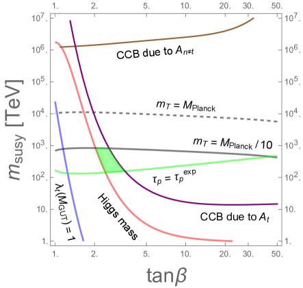
Figure 3: A naive estimate of the allowed parameter space of the minimal renormalizable supersymmetric SU(5) model (pale green region) in the approximation described in the text, where all sfermions are assumed to have the same mass $m_{susy}$.

• the measured Higgs boson mass excludes the region below the red curve (which corresponds to maximal stop mixing);

• the region below the green line is ruled out by the experimental lower bound on the proton lifetime (assuming the high-energy phases appearing in the proton decay amplitude, see Eq. (B.7), all vanish). The shape of this line can be understood by noting that the proton lifetime approximately scales as

  $$\tau(p\to K^{+}\bar{\nu})\,\propto\,m_{T}^{2}\,m_{susy}^{2}\tan^{2}\beta/(1+\tan^{2}\beta)^{2}\,,$$ (7.1)

  while given the assumptions made on the superpartner spectrum, the colour triplet mass is proportional to

  $$m_{T}\,\propto\,m_{susy}^{5/6}\,(\tan^{2}\beta+1)^{1/12}\,,$$ (7.2)

  giving

  $$\tau(p\to K^{+}\bar{\nu})\,\propto\,m_{susy}^{11/3}\,\tan^{2}\beta\,(\tan^{2}\beta+1)^{-11/6}\ ;$$ (7.3)

• the region above the purple curve is excluded by the vacuum metastability constraint on $A_{t}$, while the region above the brown curve (which is almost entirely due to $A_{b}$) is ruled out by the constraints on all other $A$-terms. In drawing these curves we used the metastability conditions derived in Appendix D, but they can be approximated to a very good degree by:

  $$|A_{t}|\,<\,\sqrt{m_{H_{u}}^{2}+m_{\tilde{Q}_{3}}^{2}+m_{\tilde{u}_{3}}^{2}}\ ,\qquad|A_{b}|\,<\,\sqrt{m_{H_{d}}^{2}+m_{\tilde{Q}_{3}}^{2}+m_{\tilde{d}_{3}}^{2}}\ ,$$ (7.4)

  for $A_{t}$ and $A_{b}$, respectively. Note that the constraint on $|A_{b}|$ is more easily satisfied for large $\tan\beta$ values due to $m^{2}_{H_{d}}=m^{2}_{susy}(2\tan^{2}\beta-1)$;

• perturbativity of the top quark Yukawa coupling excludes the region to the left of the blue curve (which corresponds to $\lambda_{t}(M_{GUT})=1$). There is no similar constraint for $\lambda_{b}$ and $\lambda_{\tau}$, which are always in the perturbative regime in the region of the parameter space shown in Fig. 3;

• the constraint $m_{T}<M_{Planck}/10$ (resp. $m_{T}<M_{Planck}$) rules out $m_{susy}$ values above the solid black line (resp. the dashed black line), while there are no additional constraints from $m_{3},m_{8},m_{T}<m_{V}<M_{Planck}/10$;

• the pale green area is the region of the parameter space that is allowed by all the above constraints.

The tentative conclusion one can draw from Fig. 3, even though the assumptions made on the soft terms are not consistent with SU(5)-invariant boundary conditions at the GUT scale, is that viable points satisfying all phenomenological and theoretical constraints are likely to be found in the region bounded by $2\mathrel{\hbox to0.0pt{\lower 4.0pt\hbox{\hskip 1.0pt$\sim$}\hss}\raise 1.0pt\hbox{$<$}}\tan{\beta}\mathrel{\hbox to0.0pt{\lower 4.0pt\hbox{\hskip 1.0pt$\sim$}\hss}\raise 1.0pt\hbox{$<$}}5$ and $100\,\mathrm{TeV}\mathrel{\hbox to0.0pt{\lower 4.0pt\hbox{\hskip 1.0pt$\sim$}\hss}\raise 1.0pt\hbox{$<$}}m_{susy}\mathrel{\hbox to0.0pt{\lower 4.0pt\hbox{\hskip 1.0pt$\sim$}\hss}\raise 1.0pt\hbox{$<$}}1000\,\mathrm{TeV}$. This definitely needs confirmation from a more careful investigation of the parameter space. Namely, one should scan over the parameters of the model, which besides $\tan\beta$, $\mbox{sign}(\mu)$ and the heavy state masses include 15 soft terms: 8 sfermion ($m_{10_{1,2,3}}$, $m_{\bar{5}_{1,2,3}}$) and Higgs ($m_{5}$, $m_{\bar{5}}$) soft masses, 1 gaugino mass parameter ($M_{1/2}$) and 6 A-terms ($A^{10}_{1,2,3}$, $A^{\bar{5}}_{1,2,3}$). Since these soft parameters are defined at the GUT scale, one needs to run them down to the scale $m_{susy}$, where most constraints apply. In order to simplify the problem, we shall use the semi-analytic approximate solutions to the soft term RGEs derived in Section 4. This will allow us to trade the GUT-scale soft parameters for low-energy ones (namely the $m_{susy}$ values of the running parameters $M_{3}$, $A_{u,c,t}$, $A_{d,s,b}$ and of 8 suitably chosen soft scalar masses) and to use the constraints at $m_{susy}$ to effectively reduce the number of free parameters.

Let us describe more precisely the procedure that we are going to employ:

1. first choose a random point in the $(\tan\beta,m_{susy})$ plane (where $m_{susy}$ is now the matching scale between the SM and the MSSM), together with $\mbox{sign}(\mu)$ and some sensible values of $M_{GUT}$, $m_{T}$ and $m_{V}$;

2. solve numerically the 2-loop MSSM RGEs for the gauge and Yukawa couplings (taking into account the GUT-scale relations (3.37) and the heavy threshold corrections to Yukawa couplings (3.47), as explained in Subsection 4.1). Then, following the procedure of Section 4, express the running soft terms at an arbitrary scale as algebraic combinations of the $m_{susy}$ values of $M_{3}$, $A_{u,c,t}$, $A_{d,s,b}$, $m^{2}_{\tilde{Q}_{1,2,3}}$, $m^{2}_{\tilde{d}^{c}_{1,2,3}}$, $m^{2}_{\tilde{u}^{c}_{3}}$ and $|\mu|^{2}$, which through the EWSB condition (3.62) can be written as a linear combination of $m^{2}_{H_{u}}(m_{susy})$ and $m^{2}_{H_{d}}(m_{susy})$;

3. impose the following 8 constraints on the $m_{susy}$ values of the soft terms: (i) the definition of the matching scale $m_{susy}\equiv\sqrt{m_{\tilde{Q}_{3}}(m_{susy})m_{\tilde{u}^{c}_{3}}(m_{susy})}$; (ii)-(iii) the equality of the first and second generation soft sfermion masses, which for simplicity we impose at the scale $m_{susy}$ rather than $M_{GUT}$: $m^{2}_{\tilde{Q}_{1}}(m_{susy})=m^{2}_{\tilde{Q}_{2}}(m_{susy})$ and $m^{2}_{\tilde{d}^{c}_{1}}(m_{susy})=m^{2}_{\tilde{d}^{c}_{2}}(m_{susy})$; (iv) the gauge coupling unification condition (3.1.1), in which $m_{T}$ and $M_{GUT}$ are fixed and $\mu$ and $m_{A}$ are functions of $m^{2}_{H_{u}}$ and $m^{2}_{H_{d}}$ through the EWSB conditions; (v) the 1-loop matching condition for the Higgs quartic coupling (3.48), keeping as a first approximation only the leading term (3.49); (vi)-(viii) the supersymmetric threshold corrections (3.38) needed for the down-type quark masses to match their measured values. Whenever these constraints admit several solutions, we explore all of them. Imposing them allows us to express 8 of the 15 input parameters at the scale $m_{susy}$ in terms of the remaining 7 ones and of already known quantities; in practice we choose the remaining 7 free parameters (the ones to which we assign random values in order to explore the model parameter space) to be $m_{\tilde{Q}_{1,3}}(m_{susy})$, $m_{\tilde{d}^{c}_{1,3}}(m_{susy})$, $M_{3}(m_{susy})$ and $A_{u,c}(m_{susy})$.

4. for each point of the parameter space, defined by the chosen values of $m_{\tilde{Q}_{1,3}}(m_{susy})$, $m_{\tilde{d}^{c}_{1,3}}(m_{susy})$, $M_{3}(m_{susy})$ and $A_{u,c}(m_{susy})$ (in addition to the values of $\tan\beta$, $m_{susy}$, $M_{GUT}$, $m_{T}$ and $m_{V}$, already fixed in the first step), one can improve the analysis by running the soft terms again, this time with the full RGEs, and use the complete expression for the Higgs mass. Once this is done, the phenomenological viability of this point must be further checked: proton lifetime, consistency of the superpartner mass spectrum with the experimental limits, absence of UFB directions and metastability of the electroweak vacuum (which is checked following the procedure described in Appendix D), perturbativity constraints.

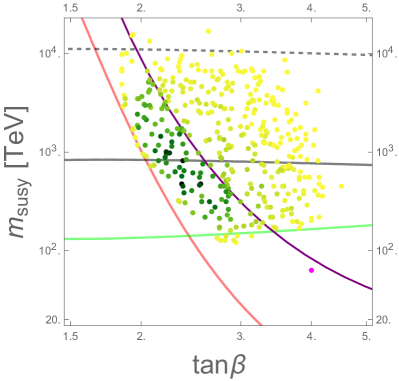
Figure 4: Left panel: successful (green dots) and unsuccessful (red stars) points among 1000 randomly selected points in the $(\tan\beta,m_{susy})$ plane. Right panel: successful points only, where the colour of a given dot represents the number of superpartner spectrum configurations respecting SU(5) symmetry at $M_{GUT}$ that passed all phenomenological constraints (the number of solutions found increases from light yellow to dark green). Also shown is a particular solution (magenta dot) characterized by a low value of the matching scale $m_{susy}\equiv\sqrt{m_{\tilde{Q}_{3}}(m_{susy})\,m_{\tilde{u}^{c}_{3}}(m_{susy})}$ and described in greater detail in the text below. In both panels, the red, green, purple and black lines represent the naive constraints from Fig. 3 associated with the measured Higgs mass, the proton lifetime, the metastability of the electroweak vacuum and the condition $m_{T}<M_{Planck}/10$, respectively.

The procedure described above was applied by testing each randomly chosen point in the $(\tan\beta,m_{susy})$ plane for 1000 different random configurations of the superpartner spectrum, which were obtained by scanning over $m_{\tilde{Q}_{1,3}}(m_{susy})$, $m_{\tilde{d}^{c}_{1,3}}(m_{susy})$ and $M_{3}(M_{GUT})$ in the range $[0.5\,m_{susy},2\,m_{susy}]$, and over $A_{u,c}(m_{susy})$ in the range $[-2\,m_{susy},2\,m_{susy}]$. The results of this exploration of the parameter space of the minimal renormalizable supersymmetric SU(5) model can be seen in Fig. 4. The plot in the left panel displays all the points of the $(\tan\beta,m_{susy})$ plane that have been checked; the ones for which at least one configuration of the superpartner spectrum passed all constraints are in green, while the ones that failed this test are in red. The plot in the right panel shows how frequently a solution was found in the model parameter space for each green point. The more vivid the colour of the point, the more spectrum configurations survived all the constraints. It turns out that the naive estimate of the allowed parameter space (the green region in Fig. 3), despite not respecting the SU(5) symmetry, tells us something about how likely it is for a randomly chosen point in the parameter space with given values of $\tan{\beta}$ and $m_{susy}$ to be compatible with all experimental and theoretical constraints discussed at the beginning of this section. In the part of the green region of Fig. 3 around several hundreds of TeV (close to the upper limit given by the requirement $m_{T}\leq M_{Planck}/10$), a randomly chosen point in the parameter space has a few percent probability of success, while the probability decreases when one exits the green region. One can see that the naive constraints associated with the Higgs mass (red line) and with the proton lifetime (green line) are very robust, which in the case of the Higgs mass can be traced back to the fact that the leading term in the 1-loop matching condition for the Higgs quartic coupling, Eq. (3.49), only depends on $m_{susy}$ in the maximal stop mixing case. The naive vacuum metastability bound (purple line) is less robust but remains a reasonable approximation to the exact condition, contrary to the naive $m_{T}<M_{Planck}/10$ constraint (black line). The main reason for this is that the black line assumed $\mu(m_{susy})=m_{susy}$, while a sizable portion of the viable points of the parameter space feature smaller values of $\mu$, thus effectively decreasing the value of $m_{T}$ by virtue of the gauge coupling unification condition (3.1.1).

While these results confirm the naive expectation from Fig. 3 that the allowed parameter space of the minimal renormalizable supersymmetric SU(5) model is restricted to the region of heavy superpartners, isolated points with lighter supersymmetric particles are likely to be missed in this random search. In fact we were able to find a viable point in the parameter space with $m_{susy}=63\,\mathrm{TeV}$ and some squarks as light as $22\,\mathrm{TeV}$, depicted by a magenta dot in Fig. 4. We give below the input parameters at the GUT scale as well as the values of all soft terms at the scale $m_{susy}$:

INPUT: Point in the $(\tan\beta,m_{susy})$ plane:

$$\tan\beta \ =\ 4.0\,,$$ (7.5)

$$m_{susy} \ =\ 63.0\,\mathrm{TeV}\,,$$ (7.6)

$$M_{GUT} \ =\ 2.0\times 10^{16}\,\mathrm{GeV}\,,$$ (7.7)

$$\mbox{sign}(\mu) \ =\ +\,,$$ (7.8)

Soft terms at $\mathbf{M_{GUT}}$:

$$A_{u}(M_{GUT}) \ =\ \mbox{Diag}\,(2\times 10^{-4},9\times 10^{-2},13.9)\,\mathrm{TeV}\,,$$ (7.9)

$$A_{d}(M_{GUT})\,=\,A_{e}(M_{GUT}) \ =\ \mbox{Diag}\,(-0.4,41.2,121.7)\,\mathrm{TeV}\,,$$ (7.10)

$$M_{1/2} \ =\ 34.4\,\mathrm{TeV}\,,$$ (7.11)

$$m_{H_{u}}(M_{GUT}) \ =\ 106.2\,\mathrm{TeV}\,,$$ (7.12)

$$m_{H_{d}}(M_{GUT}) \ =\ 531.2\,\mathrm{TeV}\,,$$ (7.13)

$$m_{10_{i}} \ =\ \mbox{Diag}\,(79.9,79.9,125.7)\,\mathrm{TeV}\,,$$ (7.14)

$$m_{\bar{5}_{i}} \ =\ \mbox{Diag}\,(151.8,151.8,141.1)\,\mathrm{TeV}\,.$$ (7.15)

OUTPUT: Values of gauge and Yukawa couplings at $\mathbf{m_{susy}}$, in the supersymmetric ($m_{susy}+\epsilon$) and in the non-supersymmetric theory ($m_{susy}-\epsilon$):

$$g_{i}(m_{susy}+\epsilon) \ =\ (0.47777,\,0.61950,\,0.88966)\,,$$ (7.16)

$$g_{i}(m_{susy}-\epsilon) \ =\ (0.47777,\,0.61900,\,0.88742)\,,$$ (7.17)

$$(\lambda_{t},\lambda_{b},\lambda_{\tau})(m_{susy}+\epsilon) \ =\ (0.74778,\,0.06325,\,0.04229)\,,$$ (7.18)

$$(h_{t},h_{b},h_{\tau})(m_{susy}-\epsilon) \ =\ (0.72553,\,0.01123,\,0.01026)\,,$$ (7.19)

$$(\lambda_{c},\lambda_{s},\lambda_{\mu})(m_{susy}+\epsilon) \ =\ (2.61\times 10^{-3},\,3.95\times 10^{-3},\,2.52\times 10^{-3})\,,$$ (7.20)

$$(h_{c},h_{s},h_{\mu})(m_{susy}-\epsilon) \ =\ (2.53\times 10^{-3},\,0.23\times 10^{-3},\,0.61\times 10^{-3})\,,$$ (7.21)

$$(\lambda_{u},\lambda_{d},\lambda_{e})(m_{susy}+\epsilon) \ =\ (5\times 10^{-6},\,19\times 10^{-6},\,12\times 10^{-6})\,,$$ (7.22)

$$(h_{u},h_{d},h_{e})(m_{susy}-\epsilon) \ =\ (5\times 10^{-6},\,12\times 10^{-6},\,3\times 10^{-6})\,,$$ (7.23)

Soft terms at $\mathbf{m_{susy}}$:

$$A_{u}(m_{susy}) \ =\ \mbox{Diag}\,(0,0,-25.9)\,\mathrm{TeV}\,,$$ (7.24)

$$A_{d}(m_{susy}) \ =\ \mbox{Diag}\,(-0.9,87.6,237.2)\,\mathrm{TeV}\,,$$ (7.25)

$$A_{e}(m_{susy}) \ =\ \mbox{Diag}\,(-0.6,55.8,163.4)\,\mathrm{TeV}\,,$$ (7.26)

$$M_{i}(m_{\tilde{g}}) \ =\ \mbox{Diag}\,(16.9,29.9,62.0)\,\mathrm{TeV}\,,$$ (7.27)

$$m_{H_{u}}(m_{susy}) \ =\ 82.1\,\mathrm{TeV}\,,$$ (7.28)

$$m_{H_{d}}(m_{susy}) \ =\ 483.5\,\mathrm{TeV}\,,$$ (7.29)

$$m_{\tilde{Q}_{i}}(m_{susy}) \ =\ \mbox{Diag}\,(106.2,100.0,81.4)\,\mathrm{TeV}\,,$$ (7.30)

$$m_{\tilde{u}^{c}_{i}}(m_{susy}) \ =\ \mbox{Diag}\,(22.3,22.3,49.0)\,\mathrm{TeV}\,,$$ (7.31)

$$m_{\tilde{e}^{c}_{i}}(m_{susy}) \ =\ \mbox{Diag}\,(138.0,132.1,120.1)\,\mathrm{TeV}\,,$$ (7.32)

$$m_{\tilde{L}_{i}}(m_{susy}) \ =\ \mbox{Diag}\,(131.4,128.3,84.4)\,\mathrm{TeV}\,,$$ (7.33)

$$m_{\tilde{d}^{c}_{i}}(m_{susy}) \ =\ \mbox{Diag}\,(172.0,164.4,76.5)\,\mathrm{TeV}\,,$$ (7.34)

$$\mu(m_{susy}) \ =\ 91.6\,\mathrm{TeV}\,,$$ (7.35)

$$m_{A}(m_{susy}) \ =\ 507.3\,\mathrm{TeV}\,,$$ (7.36)

Values of gauge and Yukawa couplings at $\mathbf{M_{GUT}}$:

$$g^{MSSM}_{i}(M_{GUT}) \ =\ (0.68367,\,0.67083,\,0.66722)\,,$$ (7.37)

$$g_{GUT} \ =\ 0.71339\,,$$ (7.38)

$$(\lambda_{t},\lambda_{b},\lambda_{\tau})(M_{GUT}) \ =\ (0.51487,\,0.03185,\,0.03132)\,,$$ (7.39)

$$(\lambda_{c},\lambda_{s},\lambda_{\mu})(M_{GUT}) \ =\ (1.47\times 10^{-3},\,1.86\times 10^{-3},\,1.86\times 10^{-3})\,,$$ (7.40)

$$(\lambda_{u},\lambda_{d},\lambda_{e})(M_{GUT}) \ =\ (3\times 10^{-6},\,9\times 10^{-6},\,9\times 10^{-6})\,,$$ (7.41)

GUT state masses:

$$m_{T} \ =\ 7.1\times 10^{16}\,\mathrm{GeV}\,,$$ (7.42)

$$m_{8,3} \ =\ 5.1\times 10^{13}\,\mathrm{GeV}\,,$$ (7.43)

$$m_{V} \ =\ 8.8\times 10^{16}\,\mathrm{GeV}\,,$$ (7.44)

Other parameters and observables:

$$\alpha_{GUT}^{-1} \ =\ 24.7\,,$$ (7.45)

$$\tau_{p}(p^{+}\to K^{+}\bar{\nu}) \ =\ 3.9\times 10^{33}\textrm{ yrs}\qquad(\textrm{ for }\phi_{1}=\phi_{2}=\phi_{3}=0)\,,$$ (7.46)

$$S^{min} \ =\ 1780\,,$$ (7.47)

corresponding to a vacuum lifetime of

$$\tau_{vacuum}\,=\,\frac{e^{S^{min}}}{m_{susy}^{4}t_{universe}^{3}}\,\approx\,10^{580}\,{\rm yrs}\,.$$ (7.48)

For completeness, we also present the running of the A-terms in Fig. 5 and of the soft scalar masses in Fig. 6.

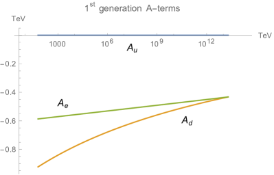
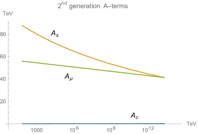
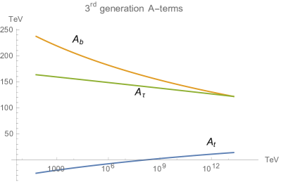
Figure 5: Running A-terms and gaugino masses for the parameter space point described in the text (magenta dot in Fig. 4), obtained using the 1-loop MSSM RGEs. Top and bottom left figures: $1^{st}$, $2^{nd}$ and $3^{rd}$ generation A-terms. The blue, yellow and green lines represent $A_{u_{i}}$, $A_{d_{i}}$ and $A_{e_{i}}$, respectively. Bottom right figure: the blue, yellow and green lines represent $M_{1}$, $M_{2}$ and $M_{3}$, respectively.

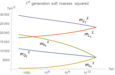
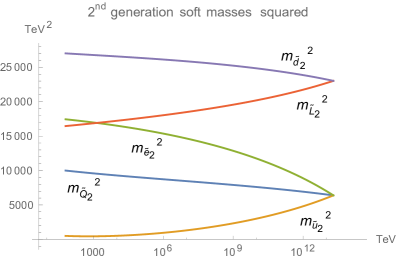
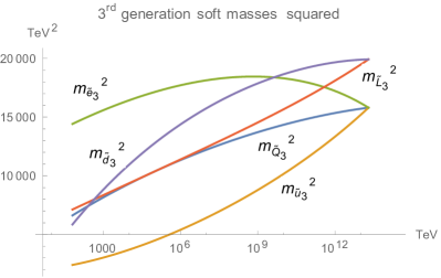
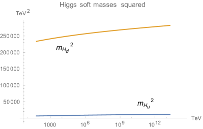
Figure 6: Running soft scalar masses for the parameter space point described in the text (magenta dot in Fig. 4), obtained using the 1-loop MSSM RGEs. Top and bottom left figures: $1^{st}$, $2^{nd}$ and $3^{rd}$ generation soft sfermion masses. The blue, yellow, green, red and purple lines represent $m^{2}_{\tilde{Q}_{i}}$, $m^{2}_{\tilde{u}^{c}_{i}}$, $m^{2}_{\tilde{e}^{c}_{i}}$, $m^{2}_{\tilde{L}_{i}}$ and $m^{2}_{\tilde{d}^{c}_{i}}$, respectively. Bottom right figure: soft Higgs boson masses. The blue line represents $m^{2}_{H_{u}}$ and the yellow line $m^{2}_{H_{d}}$.

Let us describe briefly the main features of this point. Most sfermions lie between $50$ and $170\,\mathrm{TeV}$, with however the $\tilde{u}_{R}$ and $\tilde{c}_{R}$ as light as $22.3\,\mathrm{TeV}$. The gauginos are typically lighter than the sfermions and the higgsinos, and the lightest supersymmetric particle (LSP) is the bino, with mass $M_{1}=16.9\,\mathrm{TeV}$ (the $\tilde{u}_{R}$ and the $\tilde{c}_{R}$ are the co-NLSPs, i.e. the next-to-lightest supersymmetric particles). The superpartners are therefore out of reach of present and next-generation colliders, and supersymmetric contributions to flavour physics observables are strongly suppressed, but proton decay will be easily accessible at future large detectors. The Higgs sector is far into the decoupling regime, with a standard-like lightest Higgs boson and all non-standard Higgs bosons around $m_{A}\approx 500\,\mathrm{TeV}$. Finally, there is no suitable dark matter particle in the observable sector, as the relic density of a $17\,\mathrm{TeV}$ bino by far exceeds $\Omega_{CDM}h^{2}\simeq 0.12$ [47]. If R-parity is conserved, a natural candidate is a gravitino in the GeV range (or lower), to which the bino NLSP would decay without affecting Big Bang nucleosynthesis. The cold dark matter density would then be in the form of gravitinos coming from NLSP decays [48] (giving a contribution $\Delta\Omega_{\tilde{G}}=\Omega_{\tilde{B}}m_{\tilde{G}}/M_{1}$, from which the upper bound $m_{\tilde{G}}\mathrel{\hbox to0.0pt{\lower 4.0pt\hbox{\hskip 1.0pt$\sim$}\hss}\raise 1.0pt\hbox{$<$}}1\,\mathrm{GeV}$ follows) and from thermal production during reheating [49, 50]. In order to avoid gravitino overproduction from the latter process, the reheating temperature should lie in the TeV range, or lower. In the case of R-parity violation (which may be invoked to generate neutrino masses, as an alternative to the seesaw mechanism), the only possible dark matter candidate within this model is again the gravitino. Since it decays into a photon and a neutrino, acting as a source of monochromatic photons, extragalactic gamma ray constraints put a bound on its mass. For bilinear R-parity violation, one obtains $m_{\tilde{G}}\mathrel{\hbox to0.0pt{\lower 4.0pt\hbox{\hskip 1.0pt$\sim$}\hss}\raise 1.0pt\hbox{$<$}}1\;{\rm GeV}$ [51]. Here, as in the R-parity conserving case, the maximal reheating temperature is around the TeV scale.

One may wonder whether other points exist in the parameter space of the minimal renormalizable SU(5) model with lighter superpartners than in the above example. While performing an extensive scan would probably reveal the existence of such points, it appears difficult to lower significantly the average superpartner mass scale below a few tens of $\,\mathrm{TeV}$ (some supersymmetric particles may however be accidentally lighter). The reason for this is the proton lifetime, which in the limit where all superpartners have the same mass $m_{susy}$ scales as $\tau_{p}\propto m_{T}^{2}\,m_{susy}^{2}\propto m^{11/3}_{susy}$ (where in the last step the approximate constraint (3.31) from gauge coupling unification was used). The actual proton decay constraint depends on the individual superpartner masses, and does not prevent some of them to be much smaller than the naive lower bound on $m_{susy}$, but it seems to be difficult to reconcile a significantly lighter superpartner spectrum with proton decay and all other constraints. In fact gauge coupling unification is the main obstacle here, which makes it hard to accommodate a low superpartner mass scale with a large colour triplet mass [7].

What one may still try is to split the spectrum, making just a part of it light. This is not easy though, because of the threshold corrections to gauge couplings at $M_{GUT}$ and to the bottom and Higgs masses at $m_{susy}$. For example, making the higgsino light decreases the mass of the colour triplet, see Eq. (3.1.1), and therefore shortens the proton lifetime. The gluino and/or the $\tilde{b}_{R}$ cannot be much lighter than the $\tilde{b}_{L}$ (whose mass is of order $m_{susy}$) either, since this would suppress the loop function in Eq. (3.38) and require an enormous value of $X_{b}$ to reproduce the observed $m_{b}/m_{\tau}$ ratio. This large value of $X_{b}$ would in turn imply a large negative threshold correction to the Higgs quartic coupling, see Eq. (3.50), making it impossible to fit the measured Higgs mass for moderate values of $m_{susy}$. All this motivates the choice of parameter intervals made in our scan, namely $m_{\tilde{Q}_{1,3}}(m_{susy})$, $m_{\tilde{d}^{c}_{1,3}}(m_{susy})$ and $M_{3}(M_{GUT})$ in the range $[0.5\,m_{susy},2\,m_{susy}]$. The only remaining possibility is to have the first two sfermion generations lighter than the third one, an opposite situation to the one considered e.g. in Ref. [7]. The investigation of this case would require the use of 2-loop RGEs for soft terms, as a strong mass hierarchy between different sfermion generations enhances the effect of 2-loop running and may give rise to tachyons [52]. Such a study is beyond the scope of this paper, and we leave it for future work.

8 Conclusions

If one excepts the issue of neutrino masses, the minimal renormalizable supersymmetric SU(5) model suffers from two main problems. The first one concerns the predictions for charged fermion masses. Although the GUT-scale equality of down-type quark and charged lepton Yukawa couplings leads to a qualitatively successful prediction for the bottom to tau mass ratio, it quantitatively differs from the measured value by some $20$–$30\%$, while the discrepancy is much larger for the first and second generations. Second, proton decay is too fast by a factor $10^{4}$ or so for typical soft terms in the TeV range, essentially because gauge coupling unification requires a relatively light colour triplet. Each of the two problems has been addressed separately in the literature: large supersymmetric threshold corrections were used to modify the fermion mass predictions (see for example Refs. [11, 12]); specific flavour structures of the soft terms [3] and a heavy superpartner spectrum [53] were invoked to increase the proton lifetime.

In this paper, we performed a complete analysis of the minimal renormalizable supersymmetric SU(5) model, taking into account all relevant phenomenological and theoretical constraints: charged fermion masses, the proton lifetime, gauge coupling unification, the Higgs mass, experimental lower bounds on superpartner masses and flavour constraints, metastability of the vacuum and perturbativity of the model. We showed that the model is still alive, and that the allowed region of the parameter space spreads over a large domain with $m_{susy}\equiv\sqrt{m_{\tilde{t}_{1}}m_{\tilde{t}_{2}}}$ ranging from around $50\,\mathrm{TeV}$ to $10^{4}\,\mathrm{TeV}$ and $\tan{\beta}$ from approximately $2$ to $5$. Viable points were also found outside this region of the parameter space, but they are less frequent. Particularly interesting are the ones featuring some (relatively) light superpartners. We studied in greater detail one such point in which the lightest supersymmetric particle is a bino with mass $16.9\,\mathrm{TeV}$.

A generic feature of the model is the metastability of the vacuum, which is not a concern since its lifetime is typically much larger than the age of the universe. A consequence of the heavy supertpartner spectrum is that the observable sector does not contain a suitable dark matter candidate; however, a gravitino with a mass around the GeV scale or below can play the role of cold dark matter, both in the presence and in the absence of R-parity.

The present analysis is a good starting point for further research. One of the limitations is that we used the central values of the input SM parameters; taking into account the experimental and theoretical uncertainties will extend the viable region of the parameter space. We presented in a compact way all the ingredients that are needed for a more extensive scan of the parameter space of the model. What we have shown is that the minimal renormalizable supersymmetric SU(5) model is indeed a viable extension of the Standard Model, in the sense that its parameter space contains points that satisfy all relevant phenomenological and theoretical constraints. The price to pay is that the superpartner spectrum is heavy, typically in the $100\,\mathrm{TeV}$ region or above, although we were able to find particular cases in which some of the supersymmetric particles can be as light as $17$ TeV, and it is not excluded that viable points with even more split spectra exist in some corners of the parameter space.

We did not address in this paper the issue of neutrino masses. One possibility is to add Standard Model singlets (right-handed neutrinos) to the model and to generate neutrino masses via the seesaw mechanism. Another possibility is to allow either bilinear or trilinear R-parity violating terms. Notice that integrating out higgsinos and colour triplets with R-parity violating couplings induces corrections to the Yukawa couplings [21], which opens the possibility that the SU(5) fermion mass relations are cured by the combined effect of R-parity violation and of supersymmetric threshold corrections.

The possibilities to test experimentally the minimal renormalizable supersymmetric SU(5) model are limited. Barring possible isolated points of the parameter space with light remnants, superpartners are too heavy to be detected at the next generation of colliders or to give sizable contributions to flavour-violating observables. Proton decay could be around the corner, but the allowed parameter space is too vast to give a definite prediction for the proton lifetime. It is, however, possible to rule out the model (or at least most of its allowed parameter space), either by discovering a light superpartner spectrum or, if the Higgs sector is light enough to be accessible and studied at the next generation of colliders, by measuring a relatively large value of $\tan\beta$.

Appendix A Procedure for solving the soft term RGEs

In this appendix, we derive the expressions for the superpartner spectrum of the minimal renormalizable supersymmetric SU(5) model that we have used in our analysis. These formulae account for the splitting of sfermion masses within the same SU(5) multiplet due to renormalization group running. They are (approximate) semi-analytic solutions to the 1-loop MSSM RGEs for the soft terms obtained under certain assumptions (namely, the hierarchy among Yukawa couplings allows us to neglect some terms in the RGEs and to solve them in a sequential manner, as explained below). We have checked that they are accurate up to the few percent level by running the full set of RGEs. The advantage of these approximate solutions is that the low-energy soft terms can be written as quadratic functions of the initial (GUT-scale) values of the soft parameters, which makes it possible to perform a scan over the parameter space of the model without having to solve the full set of RGEs for each point. Furthermore, it is possible to scan directly over the low-energy values of the soft terms (rather than the GUT-scale ones), since these formulae implicitly respect the SU(5) boundary conditions. A similar approach has already been employed in the past, e.g. in Ref. [26] for mSUGRA and in Ref. [27] for SU(5). Here we generalize this procedure to generation-dependent soft terms with SU(5) boundary conditions.

A.1 The procedure

In order to perform a scan over the parameter space of the minimal renormalizable supersymmetric SU(5) model, one has to solve a system of entangled differential equations describing the running of gauge, Yukawa and Higgs quartic couplings, as well as of the soft terms, which involves a large number of parameters (only in the supersymmetry breaking sector, there are upon SU(5) unification 15 parameters, namely 6 A-terms, 1 gaugino mass and 8 soft scalar masses). In addition, these parameters are subject to various phenomenological constraints defined at different scales. This makes it hard to solve the problem by brute force, and motivates the use of approximate semi-analytical solutions to the soft term RGEs.

Let us first try to circumvent the issue by solving the RGEs in steps. We first integrate numerically the system of RGEs for gauge, Yukawa and Higgs quartic couplings at the 2-loop level. Note that these couplings depend on the soft terms only through supersymmetric threshold corrections, so we can use this fact to determine the values of the relevant soft terms at the matching scale $m_{susy}$. Then we can solve the 1-loop RGEs for the soft terms – first gaugino masses, then A-terms and finally soft scalar masses. By working them out in this particular order, we are able to use in each step the knowledge of the running parameters that we have computed in the previous steps. Unfortunately this method is not efficient since one must solve the RGEs for the soft terms every time one changes the input (GUT-scale) values of the soft parameters. What we would like is to numerically solve the soft term RGEs for symbolic input values. The computational procedure described below does precisely that: when the input values of the soft parameters are changed, only the last step (out of 3) has to be re-run.

Step 1

• Choose the matching scales $m_{susy}$ and $M_{GUT}$, the ratio of the MSSM Higgs vevs $\tan\beta$ and the masses of the heavy GUT states $m_{T}$ and $m_{V}$ within the perturbative regime $m_{T}<m_{V}\ll M_{Planck}$ (note that $m_{T}$ and $m_{V}$ affect the running of the parameters only through the high-scale threshold corrections to the Yukawa couplings, so their influence is very mild).

• Run the gauge, charged lepton and up-type quark Yukawa couplings as well as the Higgs quartic coupling from their measured values at the weak scale up to the matching scale $m_{susy}$ using the 2-loop SM RGEs.

• Apply the matching conditions (3.17)–(3.19), (3.33) and (3.35) to the gauge and Yukawa couplings at the scale $m_{susy}$ and use the 2-loop MSSM RGEs to run them up to the scale $M_{GUT}$.

• Compute the down-type quark Yukawa couplings at $M_{GUT}$ from the values of the charged lepton Yukawa couplings using the SU(5) mass relation (3.37) and the GUT threshold corrections (3.47). Run them down to the scale $m_{susy}$ using the 2-loop MSSM RGEs (the supersymmetric threshold corrections to the leptonic Yukawa couplings are neglected in this procedure).

Step 2

• Solve the 1-loop MSSM RGEs for gaugino masses, taking into account the unification condition (3.58).

• Assume the hierarchy $\lambda_{t}>\lambda_{b}>\lambda_{\tau}>\lambda_{c}>\lambda_{s}>\lambda_{\mu}>\lambda_{u}>\lambda_{d}>\lambda_{e}$ and the unification of leptonic and down-type quark A-terms at the GUT scale to solve the RGEs for A-terms in a sequential way (see details in Subsection A.3.2). As a result, express the running A-terms as linear functions of the gaugino masses and of their values at the scale $m_{susy}$ (which are more convenient input parameters than their values at the GUT scale, since phenomenological constraints on A-terms apply at the scale $m_{susy}$), with coefficients depending on the running quantities determined in Step 1. In this way one does not need to run the A-terms every time one changes their initial values.

• Solve the RGEs for the soft scalar masses in a similar manner.

Step 3

• Choose the values of the input soft parameters.

• Make sure that no sfermion becomes tachyonic. Check that the values of the A-terms and soft scalar masses at $m_{susy}$ reproduce the observed values of the down-type quark masses and of the Higgs mass. Verify that all experimental lower bounds on superpartner masses and flavour constraints are satisfied.

• Check vacuum (meta)stability constraints and the proton lifetime.

A.2 Input values

All input values of the SM parameters needed for the running were taken either from Ref. [54] or from Ref. [55]:

$$M_{Planck} = 2.4\times 10^{18}\,\mathrm{GeV}\,,$$ (A.1)

$$v = 174.10362\,\mathrm{GeV}\,,$$ (A.2)

$$(m_{Z},m_{t},m_{h})^{pole} = (91.1876,\,173.10,\,125.66)\,\mathrm{GeV}\,,$$ (A.3)

$$g_{i}(m_{t}) = (0.46167,\,0.64822,\,1.1666)\,,$$ (A.4)

$$(h_{t},h_{b},h_{\tau})(m_{t}) = (0.93558,\,0.0156,\,0.0100)\,,$$ (A.5)

$$(m_{c},m_{s},m_{\mu})(m_{Z}) = (619,\,55,\,103)\,\mathrm{MeV}\,,$$ (A.6)

$$(m_{u},m_{d},m_{e})(m_{Z}) = (1.27,\,2.9,\,0.5)\,\mathrm{MeV}\,,$$ (A.7)

$$\lambda(m_{t}) = 0.25420\,,$$ (A.8)

where $g_{1,2,3}(m_{t})$, $h_{t,b,\tau}(m_{t})$ and $\lambda(m_{t})$ are evaluated at NNLO (the NNNLO pure QCD contribution is also included in $h_{t}(m_{t})$ [54]), and $h_{i}(m_{Z})=m_{i}(m_{Z})/v$ for the first and second generations of fermions.

A.3 Approximate expressions for the soft terms

In order to be able to approximately solve the 1-loop RGEs for soft terms, we shall neglect all mixings. This means that in addition to assuming that the sfermion soft terms are aligned with fermion masses at the GUT scale (see Subsection 2.1), we shall neglect the effects of the CKM matrix in the RGEs. This may not be fully justified, as the impact of $V_{CKM}$ on the running of the first two generation parameters can be significant. However, this effect is suppressed either by small Yukawa couplings or by small CKM angles and is therefore never numerically important, so we shall set $V_{CKM}=\mathbb{1}$ in the RGEs and omit the subleading Yukawa contributions.

With these assumptions, we can derive approximate semi-analytic solutions to the 1-loop RGEs for the soft terms.

A.3.1 Gaugino masses

The 1-loop RGEs for gaugino masses:

$$\frac{d}{dt}M_{i} \,=\,\frac{b_{i}^{MSSM}}{2\pi}\,\alpha_{i}\,M_{i}\,\simeq\,\frac{d\alpha_{i}}{dt}\,\frac{M_{i}}{\alpha_{i}}\,,$$ (A.9)

(where the last equality is only approximate because we run gauge couplings at 2 loops) has the following simple solution respecting SU(5) symmetry:

$$M_{i}(m) \,=\,M_{1/2}\,e^{-\int_{\ln{m}}^{\ln{M_{GUT}}}dt\,\alpha_{i}(t)\,b_{i}^{MSSM}/(2\pi)}$$

$$\,\simeq\,M_{1/2}\,\frac{\alpha_{i}(m)}{\alpha_{i}(M_{GUT})}\,\simeq\,M_{i}(m_{\tilde{g}})\,\frac{\alpha_{i}(m)}{\alpha_{i}(m_{\tilde{g}})}\,\simeq\,m_{\tilde{g}}\,\frac{\alpha_{i}(m)}{\alpha_{3}(m_{\tilde{g}})}\,\frac{\alpha_{3}(M_{GUT})}{\alpha_{i}(M_{GUT})}\,.$$ (A.10)

This solution becomes exact when the 1-loop RGEs for gauge couplings are used.

A.3.2 A-terms

For small to moderate $\tan\beta$, one can take advantage of the hierarchy among Yukawa couplings (see Subsection A.1, Step 2) to simplify the 1-loop RGEs for A-terms and to solve them in a sequential way. Namely, one can write the A-term RGEs as:

$$\frac{d}{dt}A_{n} \,=\,\frac{A_{n}}{(4\pi)^{2}}\left[\sum_{p}J^{n}_{p}\lambda^{2}_{p}-\sum_{i=1}^{3}K^{n}_{i}g_{i}^{2}\right]+\frac{\lambda_{n}}{(4\pi)^{2}}\left[2\sum_{p\neq n}J^{n}_{p}\lambda_{p}A_{p}+2\sum_{i=1}^{3}K^{n}_{i}g_{i}^{2}M_{i}\right]\,,$$ (A.11)

where the indices $n$ and $p$ run over the ordered values $\{t,b,\tau,c,s,\mu,u,d,e\}$ (such that e.g. $p<c$ means $p=t,b$ or $\tau$) and the coefficients $J^{n}_{p}$, $K^{n}_{i}$ are collected in Table 1.

$p$	$t$	$b$	$\tau$	$c$	$s$	$\mu$	$u$	$d$	$e$
$J^{t}_{p}$	$18$	$1^{*}$		$3^{*}$			$3^{*}$
$J^{b}_{p}$	$1$	$18$	$1^{*}$		$3^{*}$	$1^{*}$		$3^{*}$	$1^{*}$
$J^{\tau}_{p}$		$3$	$12$		$3^{*}$	$1^{*}$		$3^{*}$	$1^{*}$
$J^{c}_{p}$	$3$			$18$	$1^{*}$		$3^{*}$
$J^{s}_{p}$		$3$	$1$	$1$	$18$	$1^{*}$		$3^{*}$	$1^{*}$
$J^{\mu}_{p}$		$3$	$1$		$3$	$12$		$3^{*}$	$1^{*}$
$J^{u}_{p}$	$3$			$3$			$18$	$1^{*}$
$J^{d}_{p}$		$3$	$1$		$3$	$1$	$1$	$18$	$1^{*}$
$J^{e}_{p}$		$3$	$1$		$3$	$1$		$3$	$12$

$i$	$3$	$2$	$1$
$K^{t}_{i}$	$\frac{16}{3}$	$3$	$\frac{13}{15}$
$K^{b}_{i}$	$\frac{16}{3}$	$3$	$\frac{7}{15}$
$K^{\tau}_{i}$		$3$	$\frac{9}{5}$
$K^{c}_{i}$	$\frac{16}{3}$	$3$	$\frac{13}{15}$
$K^{s}_{i}$	$\frac{16}{3}$	$3$	$\frac{7}{15}$
$K^{\mu}_{i}$		$3$	$\frac{9}{5}$
$K^{u}_{i}$	$\frac{16}{3}$	$3$	$\frac{13}{15}$
$K^{d}_{i}$	$\frac{16}{3}$	$3$	$\frac{7}{15}$
$K^{e}_{i}$		$3$	$\frac{9}{5}$

Table 1: The coefficients $J^{n}_{p}$, $K^{n}_{i}$ appearing in the 1-loop RGEs for A-terms (A.11).

A superscript ^∗ on a coefficient $J^{n}_{p}$ in Table 1 indicates that we neglect the corresponding term $2J^{n}_{p}\lambda_{n}\lambda_{p}A_{p}/(4\pi)^{2}$ in the RHS of Eq. (A.11), consistently with the hierarchy of Yukawa couplings. The evolution of each A-term is then (approximately) described by a differential equation of the form

$$\frac{d}{dt}A_{n}(t) \ =\ \beta^{A}_{n}(t)\,A_{n}(t)+\gamma^{A}_{n}(t)\,,$$ (A.12)

where the coefficients $\beta^{A}_{n}(t)$ and $\gamma^{A}_{n}(t)$ depend on the gauge and Yukawa couplings, and in addition $\gamma^{A}_{n}(t)$ depends linearly on the gaugino masses and on the A-terms $A_{m}(t)$ with $m<n$. This makes it possible to solve the RGEs (A.12) sequentially, from $n=t$ to $n=e$. The solutions can be written as:

$$A_{n}(t)\ =\ A_{n}(t_{0})\;e^{\,\int_{t_{0}}^{t}dt^{\prime}\beta^{A}_{n}(t^{\prime})}\,+\ e^{\,\int_{t_{0}}^{t}dt^{\prime}\beta^{A}_{n}(t^{\prime})}\int_{t_{0}}^{t}dt^{\prime}\,\left(\gamma^{A}_{n}(t^{\prime})\,e^{-\int_{t_{0}}^{t^{\prime}}dt^{\prime\prime}\beta^{A}_{n}(t^{\prime\prime})}\right)\,,$$ (A.13)

where, by using the already obtained expressions for the $A_{m}$’s with $m<n$, the integrals of the coefficients $\beta^{A}_{n}(t)$ and $\gamma^{A}_{n}(t)$ can be computed numerically after having solved the MSSM RGEs for the gauge and Yukawa couplings. As a result, one obtains the running A-terms at an arbitrary scale as linear combinations of the 7 SU(5) soft parameters $M_{1/2}$, $A^{10}_{i}$, $A^{\bar{5}}_{i}$ ($i=1,2,3$), with numerical coefficients depending on the choice of $m_{susy}$ and $\tan\beta$ (and very mildly on $M_{GUT}$, $m_{T}$ and $m_{V}$). In practice, it will prove convenient for the exploration of the parameter space of the model to trade these GUT-scale parameters for low-energy ones, so as to express the $A_{n}(t)$ as a function of $M_{3}(m_{susy})$, $A_{d_{i}}(m_{susy})$ and $A_{u_{i}}(m_{susy})$ ($i=1,2,3$). Note that if the SU(5) boundary conditions at $M_{GUT}$ had not been imposed, the $A_{n}(t)$ would depend on 12 initial parameters, namely $M_{1,2,3}$, $A_{u_{i}}$, $A_{d_{i}}$ and $A_{e_{i}}$.

A.3.3 Soft scalar masses

One can apply a similar procedure to the 1-loop RGEs for soft scalar masses. Let us first define the following variables:

$$\Sigma_{u_{i}} \ \equiv\ m^{2}_{\tilde{Q}_{i}}+m^{2}_{\tilde{u}^{c}_{i}}+m^{2}_{H_{u}}\,,$$ (A.14)

$$\Sigma_{d_{i}} \ \equiv\ m^{2}_{\tilde{Q}_{i}}+m^{2}_{\tilde{d}^{c}_{i}}+m^{2}_{H_{d}}\,,$$ (A.15)

$$\Sigma_{e_{i}} \ \equiv\ m^{2}_{\tilde{L}_{i}}+m^{2}_{\tilde{e}^{c}_{i}}+m^{2}_{H_{d}}\,.$$ (A.16)

These combinations of masses appear on the RHS of the RGEs for soft scalar masses, and obey 1-loop RGEs of the form

$$\frac{d}{dt}\Sigma_{n}\, =\,\frac{L^{n}_{n}\lambda_{n}^{2}}{(4\pi)^{2}}\,\Sigma_{n}+\frac{1}{(4\pi)^{2}}\left[\sum_{p\neq n}L^{n}_{p}\lambda_{p}^{2}\Sigma_{p}+\sum_{p}L^{n}_{p}A_{p}^{2}-\sum_{i=1}^{3}N^{n}_{i}g_{i}^{2}M_{i}^{2}\right]\,,$$ (A.17)

where again the indices $n$ and $p$ run over the ordered values $\{t,b,\tau,c,s,\mu,u,d,e\}$ and the coefficients $L^{n}_{n}$ are collected in Table 2, while $L^{n}_{p\neq n}=2J^{n}_{p}$ and $N^{n}_{i}=4K^{n}_{i}$.

$n$	$t$	$b$	$\tau$	$c$	$s$	$\mu$	$u$	$d$	$e$
$L^{n}_{n}$	$12$	$12$	$8$	$12$	$12$	$8$	$12$	$12$	$8$

Table 2: The coefficients $L^{n}_{n}$ appearing in the 1-loop RGEs for $\Sigma_{n}$ (A.17).

Neglecting the terms $L^{n}_{p}\lambda_{p}^{2}\Sigma_{p}/(4\pi)^{2}$ ($p\neq n$) on the RHS of Eq. (A.17) when the coefficients $J^{n}_{p}$ are marked with a superscript ^∗ in Table 1, one can solve the RGEs for the $\Sigma_{n}$’s sequentially from $n=t$ to $n=e$, as we did for the A-term RGEs. Indeed, in this approximation Eq. (A.17) can be written in the form:

$$\frac{d}{dt}\Sigma_{n}(t) \ =\ \beta^{\Sigma}_{n}(t)\,\Sigma_{n}(t)+\gamma^{\Sigma}_{n}(t)\,,$$ (A.18)

where $\beta^{\Sigma}_{n}(t)$ is proportional to $\lambda_{n}^{2}(t)$, and $\gamma^{\Sigma}_{n}(t)$ is a linear combination of $g_{i}^{2}(t)M_{i}^{2}(t)$, $A_{p}^{2}(t)$ and $\lambda_{m}^{2}(t)\Sigma_{m}(t)$ with $m<n$. The solution reads:

$$\Sigma_{n}(t)\ =\ \Sigma_{n}(t_{0})\;e^{\,\int_{t_{0}}^{t}dt^{\prime}\beta^{\Sigma}_{n}(t^{\prime})}\,+\ e^{\,\int_{t_{0}}^{t}dt^{\prime}\beta^{\Sigma}_{n}(t^{\prime})}\int_{t_{0}}^{t}dt^{\prime}\,\left(\gamma^{\Sigma}_{n}(t^{\prime})\,e^{-\int_{t_{0}}^{t^{\prime}}dt^{\prime\prime}\beta^{\Sigma}_{n}(t^{\prime\prime})}\right)\,,$$ (A.19)

where the integrals involve only already known quantities, since the RGEs for the $\Sigma_{m}$’s are solved in order of increasing $m$. Using the previously obtained expressions for the running A-terms and gaugino masses, the combinations of masses $\Sigma_{n}(t)$ are then expressed as quadratic functions of the GUT-scale soft scalar masses $m_{10_{i}}$, $m_{\bar{5}_{i}}$, $m_{H_{u}}(M_{GUT})$, $m_{H_{d}}(M_{GUT})$ and of the $m_{susy}$ values of $M_{3}$, $A_{u,c,t}$ and $A_{d,s,b}$, with $t$-dependent coefficients that can be computed numerically using the known solutions to the 2-loop MSSM RGEs for gauge and Yukawa couplings.

Another combination of masses that appears in the RGEs for soft scalar masses is

$$S\ \equiv\ m^{2}_{H_{u}}-m^{2}_{H_{d}}+\operatorname{Tr}\left[m^{2}_{Q}-m^{2}_{L}-2m^{2}_{U}+m^{2}_{D}+m^{2}_{E}\right]$$

$$=\ m^{2}_{H_{u}}-m^{2}_{H_{d}}+\sum_{i=1}^{3}\left[m_{\tilde{Q}_{i}}^{2}-m_{\tilde{L}_{i}}^{2}-2m_{\tilde{u}_{i}^{c}}^{2}+m_{\tilde{d}_{i}^{c}}^{2}+m_{\tilde{e}_{i}^{c}}^{2}\right],$$ (A.20)

for which the 1-loop RGE takes the simple form:

$$\frac{d}{dt}S \,=\,\frac{66}{5}\,\frac{\alpha_{1}}{4\pi}\,S\,=\,\frac{b_{1}^{MSSM}}{2\pi}\,\alpha_{1}S\,\simeq\,\frac{d\alpha_{1}}{dt}\,\frac{S}{\alpha_{1}}\,.$$ (A.21)

The last equality is only approximate because we run gauge couplings at 2 loops. Working in the 1-loop approximation, one can solve Eq. (A.21) straightforwardly:

$$S(m)\, =\,S(M_{GUT})\,e^{-\int_{\ln m}^{\ln M_{GUT}}dt\,\alpha_{1}(t)\,b_{1}^{MSSM}/(2\pi)}$$

$$\simeq\,S(M_{GUT})\,\frac{\alpha_{1}(m)}{\alpha_{GUT}}\,=\left[m^{2}_{H_{u}}(M_{GUT})-m^{2}_{H_{d}}(M_{GUT})\right]\frac{\alpha_{1}(m)}{\alpha_{GUT}}\ ,$$ (A.22)

where we have used the fact that $S(M_{GUT})=m^{2}_{H_{u}}(M_{GUT})-m^{2}_{H_{d}}(M_{GUT})$ due to the SU(5) boundary conditions on soft scalar masses.

We now have all the ingredients needed to write the solutions to the 1-loop RGEs for soft scalar masses as:

$$\hskip-2.84544ptm_{\alpha}^{2}(m)=m_{\alpha}^{2}(M_{GUT})+\sum_{n}P^{\alpha}_{n}I_{\Sigma_{n}}(m)+\sum_{n}P^{\alpha}_{n}I_{A_{n}}(m)-\sum_{i=1}^{3}Q^{\alpha}_{i}I_{M_{i}}(m)+R^{\alpha}I_{S}(m),$$ (A.23)

where $\alpha=H_{u},H_{d},\tilde{Q}_{i},\tilde{u}^{c}_{i},\tilde{e}^{c}_{i},\tilde{L}_{i},\tilde{d}^{c}_{i}$, the numerical coefficients $P^{\alpha}_{n}$, $Q^{\alpha}_{i}$ and $R^{\alpha}$ are given in Table 3,

$\alpha$	$P^{\alpha}_{t,c,u}$	$P^{\alpha}_{b,s,d}$	$P^{\alpha}_{\tau,\mu,e}$	$Q^{\alpha}_{3}$	$Q^{\alpha}_{2}$	$Q^{\alpha}_{1}$	$R^{\alpha}$
$H_{u}$	$6$				$6$	$\frac{6}{5}$	$+\frac{3}{5}$
$H_{d}$		$6$	$2$		$6$	$\frac{6}{5}$	$-\frac{3}{5}$

$\alpha$	$P^{\alpha}_{u_{i}}$	$P^{\alpha}_{d_{i}}$	$P^{\alpha}_{e_{i}}$	$Q^{\alpha}_{3}$	$Q^{\alpha}_{2}$	$Q^{\alpha}_{1}$	$R^{\alpha}$
$\tilde{Q}_{i}$	$2$	$2$		$\frac{32}{3}$	$6$	$\frac{2}{15}$	$+\frac{1}{5}$
$\tilde{u}^{c}_{i}$	$4$			$\frac{32}{3}$		$\frac{32}{15}$	$-\frac{4}{5}$
$\tilde{e}^{c}_{i}$			$4$			$\frac{24}{5}$	$+\frac{6}{5}$
$\tilde{L}_{i}$			$2$		$6$	$\frac{6}{5}$	$-\frac{3}{5}$
$\tilde{d}^{c}_{i}$		$4$		$\frac{32}{3}$		$\frac{8}{15}$	$+\frac{2}{5}$

Table 3: The non-vanishing coefficients $P^{\alpha}_{n}$, $Q^{\alpha}_{i}$ and $R^{\alpha}$ appearing in Eq. (A.23).

and the integrals $I_{\Sigma_{n}}$, $I_{A_{n}}$, $I_{M_{i}}$ and $I_{S}$ are defined by:

$$I_{\Sigma_{n}}(m)\, \equiv\,\frac{1}{(4\pi)^{2}}\int_{\ln{m_{GUT}}}^{\ln{m}}dt\,\lambda_{n}^{2}(t)\Sigma_{n}(t)\,,$$ (A.24)

$$I_{A_{n}}(m)\, \equiv\,\frac{1}{(4\pi)^{2}}\int_{\ln{m_{GUT}}}^{\ln{m}}dt\,A_{n}^{2}(t)\,,$$ (A.25)

$$I_{M_{i}}(m)\, \equiv\,\frac{1}{(4\pi)^{2}}\int_{\ln{m_{GUT}}}^{\ln{m}}dt\,g_{i}^{2}(t)M_{i}^{2}(t)\,\simeq\,\frac{M_{1/2}^{2}}{4b_{i}^{MSSM}}\left(\frac{\alpha_{i}^{2}(m)}{\alpha_{i}^{2}(M_{GUT})}-1\right),$$ (A.26)

$$I_{S}(m)\, \equiv\,\frac{1}{(4\pi)^{2}}\int_{\ln{m_{GUT}}}^{\ln{m}}dt\,g_{1}^{2}(t)S(t)\,\simeq\,\frac{S(M_{GUT})}{2b_{1}^{MSSM}}\left(\frac{\alpha_{1}(m)}{\alpha_{1}(M_{GUT})}-1\right).$$ (A.27)

Plugging the semi-analytic expressions for $\Sigma_{n}(t)$ and $A_{n}(t)$ into Eqs. (A.24) and (A.25), one can express the running soft scalar masses as quadratic functions of the GUT-scale soft parameters $m_{10_{i}}$, $m_{\bar{5}_{i}}$, $m_{H_{u}}(M_{GUT})$, $m_{H_{d}}(M_{GUT})$ and of the $m_{susy}$ values of $M_{3}$, $A_{u,c,t}$ and $A_{d,s,b}$, with $m$-dependent coefficients that can be computed numerically.

One can further simplify Eq. (A.23) by writing $I_{\Sigma_{n}}$ as a linear combination of the differences $\Sigma_{p}(m)-\Sigma_{p}(M_{GUT})$ and of the integrals $I_{A_{p}}$ and $I_{M_{i}}$. Indeed, $\Sigma_{n}$ satisfies a 1-loop RGE of the form:

$$\frac{d}{dt}\Sigma_{n}(t) \ =\ \beta^{\Sigma}_{n}(t)\,\Sigma_{n}(t)+\gamma^{\Sigma}_{n}(t)\,,$$ (A.28)

with $\beta^{\Sigma}_{n}(t)$ equal to $12\lambda_{n}^{2}(t)/(4\pi)^{2}$ for squarks and to $8\lambda_{n}^{2}(t)/(4\pi)^{2}$ for sleptons. From this and from the definition (A.24) of $I_{\Sigma_{n}}$, one immediately deduces that

$$I_{\Sigma_{u_{i},d_{i}}}(m) \ =\ \frac{\Sigma_{u_{i},d_{i}}(m)-\Sigma_{u_{i},d_{i}}(M_{GUT})}{12}-\frac{1}{12}\int_{\ln{M_{GUT}}}^{\ln{m}}dt\,\gamma^{\Sigma}_{u_{i},d_{i}}(t)\,,$$ (A.29)

$$I_{\Sigma_{e_{i}}}(m) \ =\ \frac{\Sigma_{e_{i}}(m)-\Sigma_{e_{i}}(M_{GUT})}{8}-\frac{1}{8}\int_{\ln{M_{GUT}}}^{\ln{m}}dt\,\gamma^{\Sigma}_{e_{i}}(t)\,,$$ (A.30)

where the integrals on the RHS can be expressed in terms of $I_{\Sigma_{p}}$, $I_{A_{p}}$ and $I_{M_{i}}$, so that eventually all $I_{\Sigma_{n}}$’s can be written as linear combinations of $\Sigma_{p}(m)-\Sigma_{p}(M_{GUT})$, $I_{A_{p}}$ and $I_{M_{i}}$. This leads to the following expressions for the running soft scalar masses:

$$m_{\alpha}^{2}(m)\,=\,m_{\alpha}^{2}(M_{GUT}) +\sum_{n}T^{\alpha}_{n}\left(\Sigma_{n}(m)-\Sigma_{n}(M_{GUT})\right)$$

$$+\sum_{n}U^{\alpha}_{n}I_{A_{n}}(m)+\sum_{i=1}^{3}V^{\alpha}_{i}I_{M_{i}}(m)+R^{\alpha}I_{S}(m)\,,$$ (A.31)

with the numerical coefficients $T^{\alpha}_{n}$, $U^{\alpha}_{n}$, $V^{\alpha}_{i}$ (resp. $R^{\alpha}$) given in Table 4 (resp. Table 3).

The quantities $\Sigma_{n}(m)$, $I_{A_{n}}(m)$, $I_{M_{i}}(m)$ and $I_{S}(m)$ on the RHS of Eq. (A.31) – hence the running soft scalar masses $m^{2}_{\alpha}(m)$ – are quadratic functions of chosen initial parameters, with coefficients depending on the scale $m$, $\tan\beta$ and $m_{susy}$ (and very weakly on $M_{GUT}$, $m_{T}$ and $m_{V}$). In the above derivation, the initial parameters were taken to be the GUT-scale soft masses $m_{10_{i}}$, $m_{\bar{5}_{i}}$, $m_{H_{u}}(M_{GUT})$, $m_{H_{d}}(M_{GUT})$ and the $m_{susy}$ values of $M_{3}$, $A_{u,c,t}$ and $A_{d,s,b}$. Alternatively, one can trade the 8 GUT-scale masses $m_{10_{i}}$, $m_{\bar{5}_{i}}$, $m_{H_{u}}(M_{GUT})$ and $m_{H_{d}}(M_{GUT})$ for 8 low-energy soft scalar masses by inverting 8 of the 17 equations (A.31), so as to express all running soft parameters (soft scalar masses, gaugino masses and $A$-terms) as functions of the $m_{susy}$ value of 15 of them.

$n,i$	$t$	$b$	$\tau$	$c$	$s$	$\mu$	$u$	$d$	$e$	$3$	$2$	$1$
$T^{H_{u}}_{n}$	$\frac{1}{8}$			$\frac{1}{4}$			$\frac{1}{2}$
$U^{H_{u}}_{n}$		$-\frac{1}{4}$		$-\frac{3}{4}$	$-\frac{1}{2}$		$-\frac{9}{4}$	$-1$
$V^{H_{u}}_{i}$										$\frac{56}{3}$	$\frac{9}{2}$	$\frac{11}{6}$
$T^{H_{d}}_{n}$	$\frac{19}{1024}$	$\frac{27}{512}$	$\frac{9}{256}$	$\frac{1}{128}$	$\frac{9}{64}$	$\frac{3}{32}$	$-\frac{1}{16}$	$\frac{3}{8}$	$\frac{1}{4}$
$U^{H_{d}}_{n}$		$-\frac{19}{512}$	$-\frac{27}{256}$	$-\frac{57}{512}$	$-\frac{139}{256}$	$-\frac{117}{256}$	$-\frac{81}{512}$	$-\frac{463}{256}$	$-\frac{357}{256}$
$V^{H_{d}}_{i}$										$\frac{545}{48}$	$\frac{1263}{256}$	$\frac{9461}{3840}$
$T^{\tilde{Q}_{3}}_{n}$	$\frac{5}{36}$	$\frac{1}{6}$
$U^{\tilde{Q}_{3}}_{n}$		$-\frac{5}{18}$	$-\frac{1}{3}$	$-\frac{5}{6}$	$-1$	$-\frac{1}{3}$	$-\frac{5}{6}$	$-1$	$-\frac{1}{3}$
$V^{\tilde{Q}_{3}}_{i}$										$-\frac{112}{27}$	$-\frac{7}{3}$	$\frac{89}{135}$
$T^{\tilde{u}^{c}_{3}}_{n}$	$\frac{1}{3}$
$U^{\tilde{u}^{c}_{3}}_{n}$		$-\frac{2}{3}$		$-2$			$-2$
$V^{\tilde{u}^{c}_{3}}_{i}$										$-\frac{32}{9}$	$4$	$-\frac{44}{45}$
$T^{\tilde{e}^{c}_{3}}_{n}$	$\frac{1}{24}$	$-\frac{1}{4}$	$\frac{1}{2}$
$U^{\tilde{e}^{c}_{3}}_{n}$		$-\frac{1}{12}$	$\frac{1}{2}$	$-\frac{1}{4}$	$-\frac{3}{2}$	$-\frac{1}{2}$	$-\frac{1}{4}$	$-\frac{3}{2}$	$-\frac{1}{2}$
$V^{\tilde{e}^{c}_{3}}_{i}$										$-\frac{40}{9}$	$\frac{7}{2}$	$-\frac{137}{90}$
$T^{\tilde{L}_{3}}_{n}$	$\frac{1}{48}$	$-\frac{1}{8}$	$\frac{1}{4}$
$U^{\tilde{L}_{3}}_{n}$		$-\frac{1}{24}$	$\frac{1}{4}$	$-\frac{1}{8}$	$-\frac{3}{4}$	$-\frac{1}{4}$	$-\frac{1}{8}$	$-\frac{3}{4}$	$-\frac{1}{4}$
$V^{\tilde{L}_{3}}_{i}$										$-\frac{20}{9}$	$-\frac{17}{4}$	$\frac{79}{180}$
$T^{\tilde{d}^{c}_{3}}_{n}$	$-\frac{1}{18}$	$\frac{1}{3}$
$U^{\tilde{d}^{c}_{3}}_{n}$		$\frac{1}{9}$	$-\frac{2}{3}$	$\frac{1}{3}$	$-2$	$-\frac{2}{3}$	$\frac{1}{3}$	$-2$	$-\frac{2}{3}$
$V^{\tilde{d}^{c}_{3}}_{i}$										$-\frac{128}{27}$	$\frac{10}{3}$	$-\frac{14}{135}$
$T^{\tilde{Q}_{2}}_{n}$	$-\frac{17}{288}$	$-\frac{1}{16}$	$-\frac{1}{24}$	$\frac{5}{36}$	$\frac{1}{6}$
$U^{\tilde{Q}_{2}}_{n}$		$\frac{17}{144}$	$\frac{1}{8}$	$\frac{17}{48}$	$\frac{25}{72}$	$-\frac{1}{8}$	$-\frac{23}{48}$	$-\frac{3}{8}$	$-\frac{1}{8}$
$V^{\tilde{Q}_{2}}_{i}$										$-\frac{182}{27}$	$-\frac{103}{24}$	$\frac{41}{1080}$
$T^{\tilde{u}^{c}_{2}}_{n}$	$-\frac{1}{6}$			$\frac{1}{3}$
$U^{\tilde{u}^{c}_{2}}_{n}$		$\frac{1}{3}$		$1$	$-\frac{2}{3}$		$-1$
$V^{\tilde{u}^{c}_{2}}_{i}$										$-\frac{64}{9}$	$2$	$-\frac{14}{9}$
$T^{\tilde{e}^{c}_{2}}_{n}$	$-\frac{1}{192}$	$-\frac{3}{32}$	$-\frac{1}{16}$	$\frac{1}{24}$	$-\frac{1}{4}$	$\frac{1}{2}$
$U^{\tilde{e}^{c}_{2}}_{n}$		$\frac{1}{96}$	$\frac{3}{16}$	$\frac{1}{32}$	$\frac{41}{48}$	$\frac{13}{16}$	$-\frac{7}{32}$	$-\frac{9}{16}$	$-\frac{3}{16}$
$V^{\tilde{e}^{c}_{2}}_{i}$										$-\frac{59}{9}$	$\frac{25}{16}$	$-\frac{1559}{720}$
$T^{\tilde{L}_{2}}_{n}$	$-\frac{1}{384}$	$-\frac{3}{64}$	$-\frac{1}{32}$	$\frac{1}{48}$	$-\frac{1}{8}$	$\frac{1}{4}$
$U^{\tilde{L}_{2}}_{n}$		$\frac{1}{192}$	$\frac{3}{32}$	$\frac{1}{64}$	$\frac{41}{96}$	$\frac{13}{32}$	$-\frac{7}{64}$	$-\frac{9}{32}$	$-\frac{3}{32}$
$V^{\tilde{L}_{2}}_{i}$										$-\frac{59}{18}$	$-\frac{167}{32}$	$\frac{169}{1440}$
$T^{\tilde{d}^{c}_{2}}_{n}$	$\frac{7}{144}$	$-\frac{1}{8}$	$-\frac{1}{12}$	$-\frac{1}{18}$	$\frac{1}{3}$
$U^{\tilde{d}^{c}_{2}}_{n}$		$-\frac{7}{72}$	$\frac{1}{4}$	$-\frac{7}{24}$	$\frac{49}{36}$	$-\frac{1}{4}$	$\frac{1}{24}$	$-\frac{3}{4}$	$-\frac{1}{4}$
$V^{\tilde{d}^{c}_{2}}_{i}$										$-\frac{172}{27}$	$\frac{17}{12}$	$-\frac{83}{108}$

$n,i$	$t$	$b$	$\tau$	$c$	$s$	$\mu$	$u$	$d$	$e$	$3$	$2$	$1$
$T^{\tilde{Q}_{1}}_{n}$	$-\frac{83}{2304}$	$-\frac{3}{128}$	$-\frac{1}{64}$	$-\frac{17}{288}$	$-\frac{1}{16}$	$-\frac{1}{24}$	$\frac{5}{36}$	$\frac{1}{6}$
$U^{\tilde{Q}_{1}}_{n}$		$\frac{83}{1152}$	$\frac{3}{64}$	$\frac{83}{384}$	$\frac{203}{576}$	$\frac{13}{64}$	$\frac{73}{128}$	$\frac{335}{576}$	$-\frac{3}{64}$
$V^{\tilde{Q}_{1}}_{i}$										$-\frac{865}{108}$	$-\frac{997}{192}$	$-\frac{2101}{8640}$
$T^{\tilde{u}^{c}_{1}}_{n}$	$-\frac{1}{12}$			$-\frac{1}{6}$			$\frac{1}{3}$
$U^{\tilde{u}^{c}_{1}}_{n}$		$\frac{1}{6}$		$\frac{1}{2}$	$\frac{1}{3}$		$\frac{3}{2}$	$-\frac{2}{3}$
$V^{\tilde{u}^{c}_{1}}_{i}$										$-\frac{80}{9}$	$1$	$-\frac{83}{45}$
$T^{\tilde{e}^{c}_{1}}_{n}$	$-\frac{19}{1536}$	$-\frac{9}{256}$	$-\frac{3}{128}$	$-\frac{1}{192}$	$-\frac{3}{32}$	$-\frac{1}{16}$	$\frac{1}{24}$	$-\frac{1}{4}$	$\frac{1}{2}$
$U^{\tilde{e}^{c}_{1}}_{n}$		$\frac{19}{768}$	$\frac{9}{128}$	$\frac{19}{256}$	$\frac{139}{384}$	$\frac{39}{128}$	$\frac{27}{256}$	$\frac{463}{384}$	$\frac{119}{128}$
$V^{\tilde{e}^{c}_{1}}_{i}$										$-\frac{545}{72}$	$\frac{91}{128}$	$-\frac{14069}{5760}$
$T^{\tilde{L}_{1}}_{n}$	$-\frac{19}{3072}$	$-\frac{9}{512}$	$-\frac{3}{256}$	$-\frac{1}{384}$	$-\frac{3}{64}$	$-\frac{1}{32}$	$\frac{1}{48}$	$-\frac{1}{8}$	$\frac{1}{4}$
$U^{\tilde{L}_{1}}_{n}$		$\frac{19}{1536}$	$\frac{9}{256}$	$\frac{19}{512}$	$\frac{139}{768}$	$\frac{39}{256}$	$\frac{27}{512}$	$\frac{463}{768}$	$\frac{119}{256}$
$V^{\tilde{L}_{1}}_{i}$										$-\frac{545}{144}$	$-\frac{1445}{256}$	$-\frac{49}{2304}$
$T^{\tilde{d}^{c}_{1}}_{n}$	$\frac{13}{1152}$	$-\frac{3}{64}$	$-\frac{1}{32}$	$\frac{7}{144}$	$-\frac{1}{8}$	$-\frac{1}{12}$	$-\frac{1}{18}$	$\frac{1}{3}$
$U^{\tilde{d}^{c}_{1}}_{n}$		$-\frac{13}{576}$	$\frac{3}{32}$	$-\frac{13}{192}$	$\frac{107}{288}$	$\frac{13}{32}$	$-\frac{23}{64}$	$\frac{527}{288}$	$-\frac{3}{32}$
$V^{\tilde{d}^{c}_{1}}_{i}$										$-\frac{385}{54}$	$\frac{59}{96}$	$-\frac{4501}{4320}$

Table 4: The non-vanishing coefficients $T^{\alpha}_{n}$, $U^{\alpha}_{n}$ and $V^{\alpha}_{i}$ appearing in Eq. (A.31).

Appendix B Proton lifetime computation

In this appendix, we outline the computation of the higgsino-mediated (D=5) proton decay rate [56, 57, 33, 58] in the minimal renormalizable supersymmetric SU(5) model. Integrating out the heavy colour triplet components of the $5_{H}$ and $\bar{5}_{H}$ superfields generates the following D=5 operators:

$$\left.\frac{1}{2}\,\frac{\kappa_{ijkl}}{m_{T}}\,Q_{i}Q_{j}Q_{k}L_{l}\ \right|_{\theta^{2}}\,+\ \left.\frac{1}{2}\,\frac{\kappa^{\prime}_{ijkl}}{m_{T}}\,u^{c}_{i}u^{c}_{j}d^{c}_{k}e^{c}_{l}\ \right|_{\theta^{2}}\,+\ \mbox{h.c.}\,,$$ (B.1)

where the parameters $\kappa_{ijkl}$ and $\kappa^{\prime}_{ijkl}$ can be expressed in terms of the $SU(5)$ Yukawa couplings $\Lambda^{10}_{ij}$ and $\Lambda^{\bar{5}}_{ij}$ defined in Eq. (2.2):

$$\kappa_{ijkl}\ =\ \Lambda^{10}_{ij}\Lambda^{\bar{5}}_{lk}\,,\qquad\kappa^{\prime}_{ijkl}\ =\ \Lambda^{10}_{il}\Lambda^{\bar{5}}_{kj}-\Lambda^{10}_{jl}\Lambda^{\bar{5}}_{ki}\,,$$ (B.2)

and the contraction of gauge indices is understood. Since colour invariance implies $\kappa_{iiil}=0$ and $\kappa^{\prime}_{iikl}=0$, the dominant proton decay modes arising from the above operators involve a kaon, and in practice $p\rightarrow K^{+}\bar{\nu}$ dominates. The corresponding amplitude is obtained by “dressing” the D=5 operators of Eq. (B.1) with gaugino/higgsino loops. Over the region of the parameter space considered in this paper, the dominant contribution comes from the wino dressing of the $QQQL$ operator, and the decay rate reads:

$$\Gamma(p\rightarrow K^{+}\bar{\nu})\ =\ \frac{m_{p}}{32\pi}\left(1-\frac{m^{2}_{K^{+}}}{m^{2}_{p}}\right)^{2}\,\sum_{l}\,\left|W^{112}_{0}\,C_{112l}+W^{121}_{0}\,C_{121l}\right|^{2}\,,$$ (B.3)

where $C_{ijkl}(\mu)$ is the Wilson coefficient of the 4-fermion operator $u_{i}d_{j}d_{k}\nu_{l}$ and the hadronic parameter $W^{ijk}_{0}$ is defined by $\langle K^{+}|(u_{Li}d_{Lj})d_{Lk}|p\rangle\simeq W^{ijk}_{0}P_{L}u_{p}$, where $u_{p}$ is the proton spinor. The lattice computation of Ref. [59] gives $W^{112}_{0}(\mu=2\,\mathrm{GeV})=(0.111\pm 0.027)\,\mathrm{GeV}^{2}$ and $W^{121}_{0}(\mu=2\,\mathrm{GeV})=(0.036\pm 0.014)\,\mathrm{GeV}^{2}$, with statistical and systematic errors added in quadrature. In order to minimize the dependence of the proton decay rate on the renormalization scale $\mu$, the $C_{ijkl}$’s are evaluated at the scale $\mu=2\,\mathrm{GeV}$ rather than at $\mu=m_{p}$.

The Wilson coefficients $C_{ijkl}$ are computed at the matching scale $m_{susy}$ at which supersymmetric partners are integrated out by “dressing” the $QQQL$ operators with loops containing a wino:

$$C_{ijkl}(m_{susy})\ =\ \sum_{m,n,p}\,V_{mj}V_{nk}\,\frac{\tilde{\kappa}_{pmnl}}{m_{T}}\left(\sum_{q}V^{*}_{iq}V_{pq}\,I(\tilde{W},{\tilde{d}}_{Lq},\tilde{u}_{Lm})+\delta_{pi}\,I(\tilde{W},\tilde{u}_{Ln},\tilde{e}_{Ll})\right),$$ (B.4)

in which $V$ is the CKM matrix, the parameters $\tilde{\kappa}_{pmnl}\equiv\kappa_{pmnl}-\kappa_{nmpl}$ are expressed in the super-CKM basis in which the up quarks are mass eigenstates, and the possible misalignment between the fermion and the sfermion mass eigenstate bases is neglected. In Eq. (B.4), the CKM matrix entries and the $\tilde{\kappa}_{pmnl}$’s are renormalized at the scale $m_{susy}$. The loop function $I(\tilde{W},a,b)$ is given by:

$$I(\tilde{W},a,b)\,=\,\frac{\alpha_{2}}{4\pi}\,m_{\tilde{w}}\,I_{3}\!\left(m^{2}_{a},m^{2}_{b},m^{2}_{\tilde{w}}\right),$$ (B.5)

where the function $I_{3}(x,y,z)$ has been defined in Eq. (3.42). For equal sfermion masses ($m_{a}=m_{b}\equiv m_{susy}$), $I(\tilde{W},a,b)$ reads:

$$I(\tilde{W},a,b)\,=\,\frac{\alpha_{2}}{4\pi}\ \frac{1}{m_{susy}}\,g\left(\frac{m_{susy}^{2}}{m^{2}_{\tilde{w}}}\right),\qquad g(x)\,=\,\frac{\sqrt{x}\,(x-1-\ln x)}{(x-1)^{2}}\ .$$ (B.6)

The parameters $\tilde{\kappa}_{ijkl}$ depend on the details of the Yukawa sector of the Grand Unified Theory. In the minimal supersymmetric $SU(5)$ model, they are given by (neglecting the running between $M_{GUT}$ and the triplet mass scale):

$$\tilde{\kappa}_{ijkl}(m_{T})\,=\,\lambda_{u_{i}}e^{i\phi_{i}}\delta_{ij}V^{*}_{kl}\lambda_{e_{l}}-\lambda_{u_{j}}e^{i\phi_{j}}\delta_{jk}V^{*}_{il}\lambda_{e_{l}}\,,$$ (B.7)

where the Yukawa couplings and the CKM matrix are evaluated at the scale $m_{T}$, and the $\phi_{i}$ are high-energy phases satisfying the constraint $\phi_{1}+\phi_{2}+\phi_{3}=0$. These parameters must then be evolved down to the scale $m_{susy}$ by solving the appropriate RGEs. Neglecting the Yukawa couplings, the running simply amounts to an overall rescaling:

$$\tilde{\kappa}_{ijkl}(m_{susy})\,=\,A_{SD}\,\tilde{\kappa}_{ijkl}(m_{T})\,,$$ (B.8)

where in the minimal renormalizable supersymmetric $SU(5)$ model:

$$A_{SD}\,=\,\left(\frac{\alpha_{1}(m_{susy})}{\alpha_{1}(m_{T})}\right)^{\!-\frac{1}{33}}\!\left(\frac{\alpha_{2}(m_{susy})}{\alpha_{2}(m_{3})}\right)^{\!-3}\!\left(\frac{\alpha_{2}(m_{3})}{\alpha_{2}(m_{T})}\right)^{\!-1}\!\left(\frac{\alpha_{3}(m_{susy})}{\alpha_{3}(m_{T})}\right)^{\!+\frac{4}{3}}\!\left(\frac{m_{T}}{m_{8}}\right)^{\!\frac{2\alpha_{3}(m_{T})}{\pi}}\!\!\!.$$ (B.9)

Finally, the Wilson coefficients $C_{112l}(m_{susy})$ and $C_{121l}(m_{susy})$ must be renormalized down to the scale $\mu=2\,\mathrm{GeV}$ before being inserted into Eq. (B.3):

$$C_{112l}(\mu=2\,\mathrm{GeV}) = A^{112}_{LD}\ C_{112l}(m_{susy})\,,$$ (B.10)

$$C_{121l}(\mu=2\,\mathrm{GeV}) = A^{121}_{LD}\ C_{121l}(m_{susy})\,,$$ (B.11)

where $A^{112}_{LD}$ and $A^{121}_{LD}$ are renormalization factors given by (using the formulae of Ref. [60]):

$$A^{112}_{LD}\,=\,\frac{1}{3}\left[\,2+\left(\frac{\alpha_{2}(m_{Z})}{\alpha_{2}(m_{susy})}\right)^{-36/19}\,\right]\,A_{LD}\,,$$ (B.12)

$$A^{121}_{LD}\,=\,\frac{1}{3}\left[\,4-\left(\frac{\alpha_{2}(m_{Z})}{\alpha_{2}(m_{susy})}\right)^{-36/19}\,\right]\,A_{LD}\,,$$ (B.13)

$$A_{LD}\,=\,\left(\frac{\alpha_{3}(\mu=2\,\mathrm{GeV})}{\alpha_{3}(m_{b})}\right)^{6/25}\!\left(\frac{\alpha_{3}(m_{b})}{\alpha_{3}(m_{t})}\right)^{6/23}\!\left(\frac{\alpha_{3}(m_{t})}{\alpha_{3}(m_{susy})}\right)^{6/21}\!\left(\frac{\alpha_{2}(m_{Z})}{\alpha_{2}(m_{susy})}\right)^{45/19}\!\left(\frac{\alpha_{1}(m_{Z})}{\alpha_{1}(m_{susy})}\right)^{-1/41}\!\!.\ \ \ \$$ (B.14)

The fact that $A^{112}_{LD}\neq A^{121}_{LD}$ is due to the RG-induced mixing between 4-fermion operators with different flavour indices; when this (numerically small) mixing is neglected, $A^{112}_{LD}=A^{121}_{LD}=A_{LD}$.

Appendix C UFB constraints

In this appendix, we derive the constraints on the model parameters associated with the absence of directions along which the scalar potential is unbounded from below. In doing this we will follow Ref. [61].

C.1 UFB-1

The absence of this direction (where $H_{u}=H_{d}$ to cancel the D-terms and all other vevs are vanishing) requires

$$m_{H_{u}}^{2}+m_{H_{d}}^{2}+2|\mu|^{2}\,\geq\,2B\,,$$ (C.1)

which can be rewritten (for finite $m_{Z}$) as

$$m_{H_{d}}^{2}-m_{H_{u}}^{2}\,\geq\,m_{Z}^{2}\frac{\tan^{2}{\beta}-1}{\tan^{2}{\beta}+1}\,,$$ (C.2)

where

$$|\mu|^{2}\, =\,\frac{m_{H_{d}}^{2}-m_{H_{u}}^{2}\tan^{2}{\beta}}{\tan^{2}{\beta}-1}-\frac{m_{Z}^{2}}{2}\ ,$$ (C.3)

$$B\, =\,\frac{(m_{H_{d}}^{2}-m_{H_{u}}^{2})\tan{\beta}}{\tan^{2}{\beta}-1}-\frac{m_{Z}^{2}\tan{\beta}}{\tan^{2}{\beta}+1}\ .$$ (C.4)

Eq. (C.2) is equivalent to

$$B\,\geq\,0\,,$$ (C.5)

which is automatically satisfied by assumption. As a cross-check, one can notice that neglecting $m_{Z}$ (since we typically consider situations where $m_{H_{d,u}}^{2}\gg m_{Z}^{2}$), the constraint (C.2) reduces to:

$$m_{H_{d}}^{2}\,\geq\,m_{H_{u}}^{2},$$ (C.6)

which is again automatic since $|\mu|^{2}\geq 0$.

C.2 UFB-2

We now allow nonzero vevs for $H_{u}$, $H_{d}$ and $\tilde{\nu}$ only:

$$V\,=\,\left(m_{H_{d}}^{2}+|\mu|^{2}\right)\!H_{d}^{2}\,+\left(m_{H_{u}}^{2}+|\mu|^{2}\right)\!H_{u}^{2}\, -\,2BH_{d}H_{u}\,+\,m_{\tilde{L}}^{2}\tilde{\nu}^{2}$$

$$+\,\frac{g^{\prime 2}+g_{2}^{2}}{8}\left(H_{u}^{2}-H_{d}^{2}-\tilde{\nu}^{2}\right)^{2}.$$ (C.7)

In the limit $m_{Z}\to 0$, one can recast Eq. (C.7) into a sum of three positive terms:

$$V\,=\,\frac{\left(m_{H_{d}}^{2}-m_{H_{u}}^{2}\right)\left(H_{d}\tan{\beta}-H_{u}\right)^{2}}{\tan^{2}{\beta}-1}\,+\,m_{\tilde{L}}^{2}\tilde{\nu}^{2}\,+\,\frac{g^{\prime 2}+g_{2}^{2}}{8}\left(H_{u}^{2}-H_{d}^{2}-\tilde{\nu}^{2}\right)^{2},$$ (C.8)

hence there cannot be any minimum lower than the electroweak vacuum $V=0$. For finite $m_{Z}$ only the first term in Eq. (C.8) is modified, but this does not affect the minimization of $V$ with respect to $\tilde{\nu}$:

$$\tilde{\nu}\,\left[\,\tilde{\nu}^{2}-\left(H_{u}^{2}-H_{d}^{2}-\frac{4m_{\tilde{L}}^{2}}{g^{\prime 2}+g_{2}^{2}}\right)\,\right]\,=\,0\,.$$ (C.9)

The solution $\tilde{\nu}=0$ brings us back to the UFB-1 case, so we are only interested in the non-trivial $\tilde{\nu}\neq 0$ solution, which is however consistent only for $H_{u}^{2}>H_{d}^{2}$. One can check both analytically (using for example the command Reduce in Mathematica) and numerically that in this case there is an UFB direction only if

$$m_{H_{d}}^{2}-m_{H_{u}}^{2}<m_{Z}^{2}$$ (C.10)

(plus some extra constraints), or

$$m_{H_{d}}^{2}-m_{H_{u}}^{2}\, \geq\,m_{Z}^{2}\,,$$ (C.11)

$$m_{\tilde{L}}^{2}\, \leq\,\frac{m_{Z}^{2}}{2}\ \frac{\tan^{2}{\beta}-1}{\tan^{2}{\beta}+1}$$ (C.12)

(plus some extra constraints). Since none of these conditions is satisfied in our analysis of the minimal renormalizable supersymmetric SU(5) model, we can conclude that there are no UFB-2 directions.

Naively one could think that this conclusion may change if instead of $\tilde{\nu}\neq 0$ one would allow a nonzero $\tilde{e}=\tilde{e}^{c}$, because it contributes with the opposite sign to the D-term. This is however not the case: while the non-trivial solution $\tilde{e}=\tilde{e}^{c}\neq 0$ is now consistent for $H^{2}_{u}<H^{2}_{d}$, there is also a sign change in Eq. (C.9). Hence also in this case there are no dangerous UFB-2 direction.

C.3 UFB-3

One can avoid the UFB-3 direction (with nonzero vevs for $H_{u}$, $\tilde{\nu}$ and $\tilde{d}=\tilde{d}^{c}$) if the conditions

$$m_{H_{u}}^{2}+m_{\tilde{L}}^{2} \,>\,0$$ (C.13)

are satisfied for any of the three slepton generations.

Appendix D Decays into CCB vacua

In this appendix, we describe a method to estimate the lifetime of the electroweak vacuum in the presence of charge and colour breaking (CCB) vacua induced by large A-terms from any sector and generation. To this end, we will approximate the minimal value of the bounce action in Euclidean space [62, 63, 64]:

$$S\,=\,2\pi^{2}\int_{0}^{\infty}drr^{3}\left({\cal L}_{kin}+V\right)(\phi_{i}(r))$$ (D.1)

for the solution of the equations of motion

$$\phi_{i}^{\prime\prime}(r)+\frac{3}{r}\phi_{i}^{\prime}(r)\,=\,\frac{\partial V}{\partial\phi_{i}}\ ,$$ (D.2)

subject to the boundary conditions (describing fields sitting in the false vacuum at $r=\infty$ and tending to a lower minimum at $r=0$):

$$\phi_{i}(\infty)=\phi_{i}^{\infty}\,,\qquad\phi_{i}^{\prime}(0)=0\,.$$ (D.3)

The general problem can be solved only numerically [16, 65, 17, 66, 67, 68, 69]. We will simplify it by minimizing the bounce action along a constant direction in field space [71, 72, 70], which effectively reduces the problem to a single differential equation. This approximation provides an upper bound on the minimal value of the correct multi-field bounce action [73, 72]. This means that the points of the parameter space ruled out in this way are indeed characterized by a too short vacuum lifetime, but the method retains points that after a more careful and complete analysis would be rejected.

What we have to do is therefore to minimize an Euclidean action of the form:

$$S\,=\,2\pi^{2}\int_{0}^{\infty}dr\;r^{3}\;\left(\frac{z}{2}\phi^{\prime 2}+M_{2}^{2}\phi^{2}-M_{3}\phi^{3}+\lambda\phi^{4}\right),$$ (D.4)

where the field $\phi(r)$ parametrizes a direction in field space, and check whether its minimal value is large enough for the lifetime of the electroweak vacuum to be larger than the age of the universe, namely

$$S\,>\,400\,.$$ (D.5)

This is done by solving the equation of motion (D.2) and plugging the solution back into Eq. (D.4). A semi-analytical approximate solution for the action can be found in Ref. [74] (see also Ref. [75]):

$$S\,=\,\frac{z^{2}M_{2}^{2}}{M_{3}^{2}}\hat{S}(\kappa)\,,$$ (D.6)

where

$$\hat{S}(0)\,\approx\,45.4\,,$$ (D.7)

and

$$\kappa\,=\,\lambda\frac{M_{2}^{2}}{M_{3}^{2}}\,.$$ (D.8)

$\kappa<0$ indicates that the potential is unbounded from below, while $\kappa\geq 1/4$ ensures that the minimum at $\phi=0$ is absolutely stable. Hence we only have to check that the metastability constraint (D.5) is satisfied for $0\leq\kappa<1/4$. In this range of $\kappa$ values, one has:

$$\hat{S}(\kappa)\,\geq\,\hat{S}(0)\,\approx\,45.4\,.$$ (D.9)

D.1 An example of CCB constraint

As a concrete example, let us first consider the vacuum decay to CCB minima induced by a large A-term in the down squark sector [61]; then we will generalize the discussion to other A-terms. The relevant Lagrangian is:

$${\cal L}_{kin}\, =\,|h_{u}^{\prime}(r)|^{2}+|h_{d}^{\prime}(r)|^{2}+|\tilde{d}^{\prime}(r)|^{2}+|(\tilde{d}^{c})^{\prime}(r)|^{2}+|\tilde{e}^{\prime}(r)|^{2}+|(\tilde{e}^{c})^{\prime}(r)|^{2}\,,$$

$$V\, =\,m_{H_{u}}^{2}|h_{u}|^{2}+m_{H_{d}}^{2}|h_{d}|^{2}+m_{\tilde{Q}}^{2}|\tilde{d}|^{2}+m_{\tilde{d}}^{2}|\tilde{d}^{c}|^{2}+m_{\tilde{L}}^{2}|\tilde{e}|^{2}+m_{\tilde{e}}^{2}|\tilde{e}^{c}|^{2}$$

$$\quad+\left(A_{d}\tilde{d}^{c}\tilde{d}h_{d}-\lambda_{d}\mu^{*}\tilde{d}^{c}\tilde{d}h_{u}^{*}-Bh_{u}h_{d}+\mbox{h.c.}\right)$$

$$\quad+|\mu|^{2}\left(|h_{u}|^{2}+|h_{d}|^{2}\right)+|\lambda_{d}|^{2}\left(|\tilde{d}|^{2}|\tilde{d}^{c}|^{2}+|\tilde{d}^{c}|^{2}|h_{d}|^{2}+|h_{d}|^{2}|\tilde{d}|^{2}\right)$$

$$\quad+\frac{3g_{1}^{2}/5}{8}\left(-|h_{d}|^{2}+|h_{u}|^{2}+\frac{1}{3}|\tilde{d}|^{2}+\frac{2}{3}|\tilde{d}^{c}|^{2}-|\tilde{e}|^{2}+2|\tilde{e}^{c}|^{2}\right)^{2}$$

$$\quad+\frac{g_{2}^{2}}{8}\left(|h_{d}|^{2}-|h_{u}|^{2}-|\tilde{d}|^{2}-|\tilde{e}|^{2}\right)^{2}+\frac{g_{3}^{2}}{6}\left(|\tilde{d}|^{2}-|\tilde{d}^{c}|^{2}\right)^{2},$$ (D.10)

where $h_{u,d}$, $\tilde{d}\,(\tilde{d}^{c})$ and $\tilde{e}\ (\tilde{e}^{c})$ stand for the neutral components of the MSSM Higgs doublets, the scalar partners of the left(right)-handed down-type quarks and of the left(right)-handed charged leptons, respectively. Generation indices are omitted, and all mixing angles are neglected. Finally, the parameters $\mu$ and $B$ are determined by electroweak symmetry breaking, i.e. in the limit $m_{Z}\to 0$:

$$|\mu|^{2}\, =\,\frac{m_{H_{d}}^{2}-m_{H_{u}}^{2}\tan^{2}{\beta}}{\tan^{2}{\beta}-1}\ ,$$ (D.11)

$$B\, =\,\frac{(m_{H_{d}}^{2}-m_{H_{u}}^{2})\tan{\beta}}{\tan^{2}{\beta}-1}\ .$$ (D.12)

From now on, all quantities are assumed to be real. This is equivalent to assuming that the relative phase between $\lambda_{d}$ and $\mu$ equals (modulo $\pi$) the relative phase between $A_{d}$ and $B$ (a condition which may be realized in some scenarios of supersymmetry breaking), because in this special case all phases can be absorbed in the fields involved.

For all CCB constraints except the one associated with $A_{t}$ (which will be discussed separately) and the one associated with $A_{b}$ in the large $\tan{\beta}$ regime (which will not be considered because, in the minimal renormalizable supersymmetric SU(5) model, large values of $\tan\beta$ are excluded by a combination of constraints, see Section 7) one has $\lambda_{u,d,e}^{2}\ll g_{1,2,3}^{2}$, therefore one can impose the constraint of vanishing SU(3), SU(2) and U(1) $D$-terms [61].

As explained at the beginning of the appendix, we will search for solutions to the field equations of motion of the form:

$$(h_{u},h_{d},\tilde{d},\tilde{d}^{c},\tilde{e},\tilde{e}^{c})(r)\,=\,(H_{u},H_{d},d,d,e,e)\;\phi(r)\,,$$ (D.13)

with $H_{u}$, $H_{d}$, $d$, $e$ constant, where we have in addition imposed the SU(3) D-term constraint (which also implies that $d$ and $d^{c}$ point in the same SU(3) direction)

$$d^{c}=d$$ (D.14)

(the alternative sign choice $d^{c}=-d$ would just flip the sign of $M_{3}$, see Eq. (D.18) below, without affecting the action (D.6), which depends on $M_{3}^{2}$), as well as the compatibility of the U(1) and SU(2) D-term constraints:

$$e^{c}=e\,.$$ (D.15)

Finally, the vanishing of the SU(2) D-term:

$$-d^{2}-e^{2}+H_{d}^{2}-H_{u}^{2}\,=\,0\,,$$ (D.16)

will be considered as a constraint in the following.

With these assumptions, the coefficients of the bounce action (D.4) can be expressed as:

$$M_{2}^{2}\, =\,\left(m_{\tilde{Q}}^{2}+m_{\tilde{d}}^{2}\right)d^{2}+\left(m_{\tilde{L}}^{2}+m_{\tilde{e}}^{2}\right)e^{2}$$

$$\quad+\left(m_{H_{u}}^{2}+|\mu|^{2}\right)H_{u}^{2}+\left(m_{H_{d}}^{2}+|\mu|^{2}\right)H_{d}^{2}-2BH_{u}H_{d}\,,$$ (D.17)

$$M_{3}\, =\,-2d^{2}(A_{d}H_{d}-\lambda_{d}\mu H_{u})\,,$$ (D.18)

$$z\, =\,2\left(2d^{2}+2e^{2}+H_{u}^{2}+H_{d}^{2}\right),$$ (D.19)

$$\lambda\, =\,\lambda_{d}^{2}\,d^{2}(d^{2}+2H_{d}^{2})\,.$$ (D.20)

Notice that we chose $B>0$ (see Eq. (D.12); this amounts to fix the sign of $H_{u}H_{d}$). Without loss of generality, we can also choose

$$\lambda_{d}\,>\,0\,,\qquad H_{u}\,>\,0\,,$$ (D.21)

while the signs of $A_{d}$, $\mu$ and $H_{d}$ can in principle be arbitrary. For a given point in parameter space (for which the signs of $A_{d}$ and $\mu$ are fixed), one needs to consider both signs of $H_{d}$.

D.2 General CCB constraints

Let us now generalize the previous discussion to all CCB constraints (except for the one associated with $A_{t}$). The coefficients of the bounce action (D.4) can be written compactly as:

$$M_{2}^{2}(\psi,\bar{\psi},H,\bar{H})\, =\,M_{\psi}^{2}\psi^{2}+M_{\bar{\psi}}^{2}\bar{\psi}^{2}$$

$$\quad+\left(m_{H}^{2}+|\mu|^{2}\right)H^{2}+\left(m_{\bar{H}}^{2}+|\mu|^{2}\right)\bar{H}^{2}-2BH\bar{H}\,,$$ (D.22)

$$M_{3}(\psi,H,\bar{H})\, =\,-2\psi^{2}(A_{\psi}H-\lambda_{\psi}\mu\bar{H})\,,$$ (D.23)

$$z(\psi,\bar{\psi},H,\bar{H},c_{z})\, =\,2\left(2\psi^{2}+c_{z}\bar{\psi}^{2}+H^{2}+\bar{H}^{2}\right),$$ (D.24)

$$\lambda(\psi,H)\, =\,\lambda_{\psi}^{2}\psi^{2}(\psi^{2}+2H^{2})\,,$$ (D.25)

and the D-term constraint is given by:

$$0\,=\,-\psi^{2}+(3-2c)\bar{\psi}^{2}+H^{2}-\bar{H}^{2}\,,$$ (D.26)

where the 6 different possibilities are summarized in Table 5 (the example considered previously was case 2).

$\begin{array}[]{c||c|c|c|c||c|c|c|c|c|c|}&\psi&\bar{\psi}&H&\bar{H}&M_{\psi}^{2}&M_{\bar{\psi}}^{2}&m_{H}^{2}&m_{\bar{H}}^{2}&c_{z}&c\\ \hline\cr\hline\cr 1&d\;(=d^{c})&\nu&H_{d}&H_{u}&m_{\tilde{Q}}^{2}+m_{\tilde{d}}^{2}&m_{\tilde{L}}^{2}&m_{H_{d}}^{2}&m_{H_{u}}^{2}&1&1\\ 2&d\;(=d^{c})&e\;(=e^{c})&H_{d}&H_{u}&m_{\tilde{Q}}^{2}+m_{\tilde{d}}^{2}&m_{\tilde{L}}^{2}+m_{\tilde{e}}^{2}&m_{H_{d}}^{2}&m_{H_{u}}^{2}&2&2\\ 3&u\;(=u^{c})&\nu&H_{u}&H_{d}&m_{\tilde{Q}}^{2}+m_{\tilde{u}}^{2}&m_{\tilde{L}}^{2}&m_{H_{u}}^{2}&m_{H_{d}}^{2}&1&2\\ 4&u\;(=u^{c})&e\;(=e^{c})&H_{u}&H_{d}&m_{\tilde{Q}}^{2}+m_{\tilde{u}}^{2}&m_{\tilde{L}}^{2}+m_{\tilde{e}}^{2}&m_{H_{u}}^{2}&m_{H_{d}}^{2}&2&1\\ 5&e\;(=e^{c})&u\;(=u^{c})&H_{d}&H_{u}&m_{\tilde{L}}^{2}+m_{\tilde{e}}^{2}&m_{\tilde{Q}}^{2}+m_{\tilde{u}}^{2}&m_{H_{d}}^{2}&m_{H_{u}}^{2}&2&1\\ 6&e\;(=e^{c})&d\;(=d^{c})&H_{d}&H_{u}&m_{\tilde{L}}^{2}+m_{\tilde{e}}^{2}&m_{\tilde{Q}}^{2}+m_{\tilde{d}}^{2}&m_{H_{d}}^{2}&m_{H_{u}}^{2}&2&2\\ \hline\cr\end{array}$

Table 5: The six different cases of CCB constraints considered. The D-term constraints are given in parenthesis. Whenever $d$ and $d^{c}$ ($u$ and $u^{c}$) are involved, they point in the same SU(3)_C direction.

For each case, there are several subcases to be checked according to which generation indices are carried by the $\psi$ and $\bar{\psi}$ fields. For a given generation $\psi_{i}$ (the 2 $\psi$ fields belong to the same generation), one must consider all generation choices for the $\bar{\psi}$ fields that do not give a substantial contribution to the F-terms due to the size of the corresponding Yukawa couplings (otherwise there would be no CCB minimum lower than the electroweak vacuum). Namely,

• when a single $\bar{\psi}$ field is involved (Cases 1 and 3), all generation indices should be considered;

• when two $\bar{\psi}$ fields are involved (Cases 2, 4, 5 and 6), all combinations of two different generation indices should be considered;

• the cases of two $\bar{\psi}$ fields with the same generation index should also be considered when the Yukawa coupling of the corresponding lepton is much smaller than $\lambda_{\psi}$ (i.e. one needs to consider only generations of $\bar{\psi}$’s whose fermionic partners are lighter than the fermionic partner of $\psi$).

In practice, it is enough to check generations of the $\bar{\psi}$ fields leading to the smallest value of $M_{\bar{\psi}}^{2}$, since the bounce action increases with $M_{\bar{\psi}}^{2}$. There are thus 16 possible cases: 3 generations for case 1 with $\psi=(d,s,b)$, 3 generations for case 2 with $\psi=(d,s,b)$, 2 generations for case 3 with $\psi=(u,c)$, 2 generations for case 4 with $\psi=(u,c)$, 3 generations for case 5 with $\psi=(e,\mu,\tau)$ and 3 generations for case 6 with $\psi=(e,\mu,\tau)$.

Finally, starting from the semi-analytic approximation (D.6), it is easy to show that:

$$S\, =\,4\hat{S}(\kappa)\left[\frac{\lambda}{\lambda_{\psi}^{2}}+2\psi^{2}\left((3+c_{z}-2c)\bar{\psi}^{2}+H^{2}\right)+\left((3+c_{z}-2c)\bar{\psi}^{2}+2H^{2}\right)^{2}\,\right]\frac{M_{2}^{2}}{M_{3}^{2}}$$

$$\geq\,4\hat{S}(\kappa)\frac{\kappa}{\lambda_{\psi}^{2}}\ ,$$ (D.27)

which is very large unless $\kappa$ is very small. Thus only very small values of $\kappa$ may lead to a short vacuum lifetime, and we can approximate $\hat{S}(\kappa)\simeq\hat{S}(0)\approx 45.4$. To a good approximation, the quantity that we have to minimize is therefore

$${\cal S}\,\equiv\,\frac{S}{\hat{S}(0)}\,=\,\frac{z^{2}M_{2}^{2}}{M_{3}^{2}}(\psi,\bar{\psi},H,\bar{H},c,c_{z})\,,$$ (D.28)

subject to the D-term constraint (D.26), and we must check whether

$${\cal S}^{min}\,\gtrsim\,\frac{400}{45.4}\,\approx\,9\,,$$ (D.29)

hereafter referred to as the metastability constraint. This condition must be satisfied for all six cases in Table 5 to be able to conclude (within our approximate method) that the lifetime of the electroweak vacuum is longer than the age of the universe.

Notice that one needs to minimize $\cal S$ with respect to two variables only. Indeed, one of the variables $\psi,\bar{\psi},H,\bar{H}$ is fixed by the D-term constraint (D.26), and the quantity (D.28) only depends on ratios of fields. The minimization is performed numerically. A point of the parameter space is admitted if the bounce action satisfies Eq. (D.29) in all cases listed in Table 5.

The D-term constraint (D.26) is most easily taken into account in the minimization of $\cal S$ by choosing a suitable parametrization of its general solution, for instance:

D.2.1 Cases 1, 4, 5 ($c=1$)

For $c=1$, the most general solution of Eq. (D.26) can be parametrized as:

$$H\, =\,s_{H}\bar{H}\cosh{\theta}\cos{\alpha}\,,$$ (D.30)

$$\bar{\psi}\, =\,\bar{H}\cosh{\theta}\sin{\alpha}\,,$$ (D.31)

$$\psi\, =\,\bar{H}\sinh{\theta}\,,$$ (D.32)

with $s_{H}=\pm 1$, $\theta\in[0,\infty[$ and $\alpha\in[0,\pi/2]$. The actual value of $\bar{H}\neq 0$ is irrelevant, as (D.28) only depends on ratios of fields.

D.2.2 Cases 2, 3, 6 ($c=2$)

For $c=2$, the most general solution of Eq. (D.26) can be parametrized as:

$$H\, =\,s_{H}\bar{H}\cosh{\theta}\,,$$ (D.33)

$$\bar{\psi}\, =\,\bar{H}\sinh{\theta}\sin{\alpha}\,,$$ (D.34)

$$\psi\, =\,\bar{H}\sinh{\theta}\cos{\alpha}\,,$$ (D.35)

with again $s_{H}=\pm 1$, $\theta\in[0,\infty[$ and $\alpha\in[0,\pi/2]$. As in the previous case, the actual value of $\bar{H}\neq 0$ is irrelevant.

D.3 The special case of the stop

In this case too we will make suitable approximations for estimating the minimal value of the bounce action (for more details on the subject, see Refs. [17, 76, 77, 78, 79]). As explained in Ref. [61], one cannot assume exact cancellation of the D-terms here, but we will nevertheless stick to the relatively good approximation of vanishing SU(3) D-terms, namely $\tilde{t}=\tilde{t}^{c}$. Keeping the contributions of all other fields, one can write:

$${\cal L}_{kin}\, =\,|h_{u}^{\prime}(r)|^{2}+|h_{d}^{\prime}(r)|^{2}+2|\tilde{t}^{\prime}(r)|^{2}\,,$$

$$V\, =\,m_{H_{u}}^{2}|h_{u}|^{2}+m_{H_{d}}^{2}|h_{d}|^{2}+\left(m_{\tilde{Q}}^{2}+m_{\tilde{t}}^{2}\right)|\tilde{t}|^{2}$$

$$\quad+\left(A_{t}\tilde{t}^{2}h_{u}-\lambda_{t}\mu^{*}\tilde{t}^{2}h_{d}^{*}-Bh_{u}h_{d}+\mbox{h.c.}\right)$$

$$\quad+\,|\mu|^{2}\left(|h_{u}|^{2}+|h_{d}|^{2}\right)+|\lambda_{t}|^{2}\left(|\tilde{t}|^{4}+2|\tilde{t}|^{2}|h_{u}|^{2}\right)$$

$$\quad+\,\frac{g^{\prime 2}+g_{2}^{2}}{8}\left(|h_{d}|^{2}-|h_{u}|^{2}+|\tilde{t}|^{2}\right)^{2}\,.$$ (D.36)

Assuming again all quantities to be real, we take the same ansatz as for the other CCB constraints:

$$(h_{u},h_{d},\tilde{t})(r)\,=\,(H_{u},H_{d},t)\;\phi(r)\,,$$ (D.37)

with $H_{u}$, $H_{d}$ and $t$ constant. From this we obtain:

$$M_{2}^{2}\, =\,\left(m_{\tilde{Q}}^{2}+m_{\tilde{t}}^{2}\right)t^{2}+\left(m_{H_{u}}^{2}+|\mu|^{2}\right)H_{u}^{2}+\left(m_{H_{d}}^{2}+|\mu|^{2}\right)H_{d}^{2}-2BH_{u}H_{d}\,,$$ (D.38)

$$M_{3}\, =\,-2t^{2}(A_{t}H_{u}-\lambda_{t}\mu H_{d})\,,$$ (D.39)

$$z\, =\,2\left(2t^{2}+H_{u}^{2}+H_{d}^{2}\right),$$ (D.40)

$$\lambda\, =\,\lambda_{t}^{2}t^{2}(t^{2}+2H_{u}^{2})+\frac{g^{\prime 2}+g_{2}^{2}}{8}\left(H_{u}^{2}-H_{d}^{2}-t^{2}\right)^{2}.$$ (D.41)

Due to the large Yukawa coupling of the top quark, we also have to check the lifetime of the electroweak vacuum for sizable values of $\kappa$, as opposed to the previous cases. Hence we can no longer approximate $\hat{S}(\kappa)$ by $\hat{S}(0)$, and we must minimize the following (normalized) bounce action:

$${\cal S}\,=\,\left(1+\frac{f(\kappa)-f(0)}{\hat{S}(0)}\right)\frac{z^{2}M_{2}^{2}}{M_{3}^{2}}\,,$$ (D.42)

with [74]

$$f(\kappa)\,=\,\frac{\pi^{2}/6}{(1-4\kappa)^{3}}+\frac{16.5}{(1-4\kappa)^{2}}+\frac{28}{1-4\kappa}\,,$$ (D.43)

and $\hat{S}(0)\approx 45.4$. The minimization goes again over two variables, for example the ratios $H_{u}/t$ and $H_{d}/t$, and is done numerically. It is important to keep in mind that $\cal S$ should be minimized only over the range $0\leq\kappa<1/4$, for which the potential is metastable. For $\kappa<0$ the potential is unbounded from below and for $M_{2}^{2}<0$ it is unstable, while for $\kappa\geq 1/4$ the electroweak vacuum is the global minimum of the model.

D.4 How to improve the estimate

We can improve the estimates described above in several ways:

• on top of the 6 cases described in Table 5, one could consider the case where both $\phi$ and $\bar{\phi}$ are leptons. One would then need to perform a minimization with respect to three fields, since there is no constraint due to SU(3) D-terms;

• one could consider more general radius-dependent directions in field space, which would require the use of numerical algorithms as in Ref. [69];

• we have calculated transitions between vacua of the tree-level scalar potential at the fixed scale $m_{susy}$. To improve our estimates higher order corrections and/or RG-improved potentials should be considered. Such corrections can be relevant in some cases [61].

All these generalizations are however quite involved and are beyond the scope of this paper.

References

• [1] S. Dimopoulos and H. Georgi, Nucl. Phys. B 193 (1981) 150.
• [2] J. L. Chkareuli and I. G. Gogoladze, Phys. Rev. D 58 (1998) 055011 [hep-ph/9803335].
• [3] B. Bajc, P. Fileviez Perez and G. Senjanovic, Phys. Rev. D 66 (2002) 075005 [hep-ph/0204311].
• [4] B. Bajc, P. Fileviez Perez and G. Senjanovic, hep-ph/0210374.
• [5] C. Bachas, C. Fabre and T. Yanagida, Phys. Lett. B 370 (1996) 49 [hep-th/9510094].
• [6] D. Emmanuel-Costa and S. Wiesenfeldt, Nucl. Phys. B 661 (2003) 62 [hep-ph/0302272].
• [7] H. Murayama and A. Pierce, Phys. Rev. D 65 (2002) 055009 [hep-ph/0108104].
• [8] L. J. Hall, V. A. Kostelecky and S. Raby, Nucl. Phys. B 267, 415 (1986).
• [9] L. J. Hall, R. Rattazzi and U. Sarid, Phys. Rev. D 50, 7048 (1994) [hep-ph/9306309, hep-ph/9306309].
• [10] R. Hempfling, Phys. Rev. D 49, 6168 (1994).
• [11] J. L. Diaz-Cruz, H. Murayama and A. Pierce, Phys. Rev. D 65 (2002) 075011 [hep-ph/0012275].
• [12] T. Enkhbat, arXiv:0909.5597 [hep-ph].
• [13] M. Iskrzynski, Eur. Phys. J. C 75, no. 2, 51 (2015) [arXiv:1408.2165 [hep-ph]].
• [14] A. Anandakrishnan, B. C. Bryant and S. Raby, JHEP 1505 (2015) 088 [arXiv:1411.7035 [hep-ph]].
• [15] J. M. Frere, D. R. T. Jones and S. Raby, Nucl. Phys. B 222, 11 (1983).
• [16] M. Claudson, L. J. Hall and I. Hinchliffe, Nucl. Phys. B 228 (1983) 501.
• [17] A. Kusenko, P. Langacker and G. Segre, Phys. Rev. D 54 (1996) 5824 [hep-ph/9602414].
• [18] Y. Nir and N. Seiberg, Phys. Lett. B 309 (1993) 337 [hep-ph/9304307].
• [19] L. J. Hall and M. Suzuki, Nucl. Phys. B 231 (1984) 419.
• [20] A. Y. Smirnov and F. Vissani, Nucl. Phys. B 460 (1996) 37 [hep-ph/9506416].
• [21] B. Bajc and L. Di Luzio, JHEP 1507 (2015) 123 [arXiv:1502.07968 [hep-ph]].
• [22] R. Hempfling, Nucl. Phys. B 478 (1996) 3 [hep-ph/9511288].
• [23] H. P. Nilles and N. Polonsky, Nucl. Phys. B 484 (1997) 33 [hep-ph/9606388].
• [24] M. A. Diaz, M. Hirsch, W. Porod, J. C. Romao and J. W. F. Valle, Phys. Rev. D 68 (2003) 013009 [Phys. Rev. D 71 (2005) 059904] [hep-ph/0302021].
• [25] P. Minkowski, Phys. Lett.  B 67 (1977) 421; M. Gell-Mann, P. Ramond and R. Slansky, in Supergravity, P. van Nieuwenhuizen and D.Z. Freedman (eds.), North Holland Publ. Co., 1979, p. 315; T. Yanagida, in Proc. of the Workshop on the Baryon Number of the Universe and Unified Theories, O. Sawada and A. Sugamoto (eds.), Tsukuba, Japan, 13-14 Feb. 1979, p. 95; S. L. Glashow, in Quarks and Leptons, Cargèse Lectures, 9-29 July 1979, Plenum, New York, 1980, p. 687; R. N. Mohapatra and G. Senjanovic, Phys. Rev. Lett.  44 (1980) 912.
• [26] M. Drees and M. M. Nojiri, Nucl. Phys. B 369 (1992) 54.
• [27] R. Rattazzi and U. Sarid, Phys. Rev. D 53 (1996) 1553 [hep-ph/9505428].
• [28] M. -x. Luo and Y. Xiao, Phys. Rev. Lett.  90 (2003) 011601 [hep-ph/0207271].
• [29] S. P. Martin and M. T. Vaughn, Phys. Rev. D 50 (1994) 2282 [Erratum-ibid. D 78 (2008) 039903] [hep-ph/9311340].
• [30] S. Weinberg, Phys. Lett. B 91 (1980) 51.
• [31] L. J. Hall, Nucl. Phys. B 178 (1981) 75.
• [32] Y. Yamada, Z. Phys. C 60 (1993) 83.
• [33] J. Hisano, H. Murayama and T. Yanagida, Nucl. Phys.  B 402 (1993) 46 [arXiv:hep-ph/9207279].
• [34] J. Hisano, T. Kuwahara and N. Nagata, Phys. Lett. B 723 (2013) 324 [arXiv:1304.0343 [hep-ph]].
• [35] S. Dimopoulos, S. Raby and F. Wilczek, Phys. Rev. D 24 (1981) 1681.
• [36] L. E. Ibanez and G. G. Ross, Phys. Lett. B 105 (1981) 439.
• [37] M. B. Einhorn and D. R. T. Jones, Nucl. Phys. B 196 (1982) 475.
• [38] W. J. Marciano and G. Senjanovic, Phys. Rev. D 25 (1982) 3092.
• [39] W. Martens, L. Mihaila, J. Salomon and M. Steinhauser, Phys. Rev. D 82 (2010) 095013 [arXiv:1008.3070 [hep-ph]].
• [40] S. Antusch and M. Spinrath, Phys. Rev. D 78 (2008) 075020 [arXiv:0804.0717 [hep-ph]].
• [41] J. R. Ellis, G. Ridolfi and F. Zwirner, Phys. Lett. B 257 (1991) 83.
• [42] J. R. Ellis, G. Ridolfi and F. Zwirner, Phys. Lett. B 262 (1991) 477.
• [43] E. Bagnaschi, G. F. Giudice, P. Slavich and A. Strumia, JHEP 1409 (2014) 092 [arXiv:1407.4081 [hep-ph]].
• [44] A. Delgado, M. Garcia and M. Quiros, Phys. Rev. D 90 (2014) 1, 015016 [arXiv:1312.3235 [hep-ph]].
• [45] K. A. Olive et al. [Particle Data Group Collaboration], Chin. Phys. C 38 (2014) 090001.
• [46] K. Kobayashi et al. [Super-Kamiokande Collaboration], Phys. Rev.  D 72 (2005) 052007 [arXiv:hep-ex/0502026].
• [47] P. A. R. Ade et al. [Planck Collaboration], arXiv:1502.01589 [astro-ph.CO].
• [48] S. Borgani, A. Masiero and M. Yamaguchi, Phys. Lett. B 386 (1996) 189 [hep-ph/9605222].
• [49] M. Bolz, A. Brandenburg and W. Buchmuller, Nucl. Phys. B 606 (2001) 518 [Nucl. Phys. B 790 (2008) 336] [hep-ph/0012052].
• [50] J. Pradler and F. D. Steffen, Phys. Lett. B 648 (2007) 224 [hep-ph/0612291].
• [51] F. Takayama and M. Yamaguchi, Phys. Lett. B 485 (2000) 388 [hep-ph/0005214].
• [52] N. Arkani-Hamed and H. Murayama, Phys. Rev. D 56 (1997) 6733 [hep-ph/9703259].
• [53] J. Hisano, D. Kobayashi, T. Kuwahara and N. Nagata, JHEP 1307 (2013) 038 [arXiv:1304.3651 [hep-ph]].
• [54] D. Buttazzo, G. Degrassi, P. P. Giardino, G. F. Giudice, F. Sala, A. Salvio and A. Strumia, JHEP 1312 (2013) 089 [arXiv:1307.3536].
• [55] P. Draper, G. Lee and C. E. M. Wagner, Phys. Rev. D 89 (2014) 5, 055023 [arXiv:1312.5743 [hep-ph]].
• [56] J. R. Ellis, D. V. Nanopoulos and S. Rudaz, Nucl. Phys.  B 202 (1982) 43.
• [57] P. Nath, A. H. Chamseddine and R. L. Arnowitt, Phys. Rev.  D 32 (1985) 2348.
• [58] For a review on proton decay, see e.g. P. Nath and P. Fileviez Perez, Phys. Rept.  441 (2007) 191 [arXiv:hep-ph/0601023].
• [59] Y. Aoki, E. Shintani and A. Soni, Phys. Rev. D 89 (2014) 1, 014505 [arXiv:1304.7424 [hep-lat]].
• [60] L. F. Abbott and M. B. Wise, Phys. Rev. D 22 (1980) 2208.
• [61] J. A. Casas, A. Lleyda and C. Munoz, Nucl. Phys. B 471 (1996) 3 [hep-ph/9507294].
• [62] S. R. Coleman, Phys. Rev. D 15 (1977) 2929 [Erratum-ibid. D 16 (1977) 1248].
• [63] C. G. Callan, Jr. and S. R. Coleman, Phys. Rev. D 16 (1977) 1762.
• [64] S. R. Coleman, V. Glaser and A. Martin, Commun. Math. Phys. 58 (1978) 211.
• [65] A. Kusenko, Phys. Lett. B 358 (1995) 51 [hep-ph/9504418].
• [66] J. M. Cline, G. D. Moore and G. Servant, Phys. Rev. D 60 (1999) 105035 [hep-ph/9902220].
• [67] T. Konstandin and S. J. Huber, JCAP 0606 (2006) 021 [hep-ph/0603081].
• [68] J. h. Park, JCAP 1102 (2011) 023 [arXiv:1011.4936 [hep-ph]].
• [69] C. L. Wainwright, Comput. Phys. Commun. 183 (2012) 2006 [arXiv:1109.4189 [hep-ph]].
• [70] F. Borzumati, G. R. Farrar, N. Polonsky and S. D. Thomas, Nucl. Phys. B 555 (1999) 53 [hep-ph/9902443].
• [71] I. Dasgupta, B. A. Dobrescu and L. Randall, Nucl. Phys. B 483 (1997) 95 [hep-ph/9607487].
• [72] I. Dasgupta, Phys. Lett. B 394 (1997) 116 [hep-ph/9610403].
• [73] S. R. Coleman, Nucl. Phys. B 298 (1988) 178.
• [74] U. Sarid, Phys. Rev. D 58 (1998) 085017 [hep-ph/9804308].
• [75] M. Dine, R. G. Leigh, P. Y. Huet, A. D. Linde and D. A. Linde, Phys. Rev. D 46 (1992) 550 [hep-ph/9203203].
• [76] J. E. Camargo-Molina, B. O’Leary, W. Porod and F. Staub, JHEP 1312 (2013) 103 [arXiv:1309.7212 [hep-ph]].
• [77] N. Blinov and D. E. Morrissey, arXiv:1309.7397 [hep-ph].
• [78] D. Chowdhury, R. M. Godbole, K. A. Mohan and S. K. Vempati, JHEP 1402 (2014) 110 [arXiv:1310.1932 [hep-ph]].
• [79] N. Blinov and D. E. Morrissey, JHEP 1403 (2014) 106 [arXiv:1310.4174 [hep-ph]].