Direct, nonlinear inversion algorithm for hyperbolic problems via projection-based model reduction

Abstract

We estimate the wave speed in the acoustic wave equation from boundary measurements by constructing a reduced-order model (ROM) matching discrete time-domain data. The state-variable representation of the ROM can be equivalently viewed as a Galerkin projection onto the Krylov subspace spanned by the snapshots of the time-domain solution. The success of our algorithm hinges on the data-driven Gram–Schmidt orthogonalization of the snapshots that suppresses multiple reflections and can be viewed as a discrete form of the Marchenko–Gel’fand–Levitan–Krein algorithm. In particular, the orthogonalized snapshots are localized functions, the (squared) norms of which are essentially weighted averages of the wave speed. The centers of mass of the squared orthogonalized snapshots provide us with the grid on which we reconstruct the velocity. This grid is weakly dependent on the wave speed in traveltime coordinates, so the grid points may be approximated by the centers of mass of the analogous set of squared orthogonalized snapshots generated by a known reference velocity. We present results of inversion experiments for one- and two-dimensional synthetic models.

Keywords. Gel’fand–Levitan, model reduction, optimal grids, Galerkin method, full waveform inversion

AMS Subject Classifications. 86A22, 35R30, 41A05, 65N21

1 Introduction

In seismic reflection tomography, one attempts to utilize measurements of elastic waves to create an (approximate) image of a region in the earth’s subsurface. In this paper, we present a nonlinear tomographic inversion method that can be placed within the so-called full waveform inversion (FWI) framework. Full waveform inversion algorithms employ the full equations of motion and utilize as much of the information contained in the recorded waveforms as possible to image the material properties of the region of interest [21].

The most common numerical approach to FWI is nonlinear optimization, i.e., minimization of the misfit between the measured elastic field and the forward model — see, e.g., [46, 21] (and the references within). The images created via the optimization approach tend to have high resolution; however, the conventional FWI optimization procedure suffers from a few computational and theoretical difficulties. First, the equations and models are typically discretized on a fine grid to ensure the synthetic data sets are accurately computed — the model parameters tend to be on the order of billions [21]. Even with the help of adjoint-state methods, the solution to 3D FWI problems can take days or weeks of processing time. The second difficulty with the optimization problem is that the quadratic misfit functional is nonconvex and has many local minima [21]. Gradient-based algorithms will tend to get stuck in one of these local minima, rather than the true minimum, unless the initial model is extremely close to the true model. Several approaches have been developed to mitigate the effects of the nonconvexity of the misfit functional — see [46, 21] and the references therein — though they come at a cost.

Another, direct, nonlinear approach originated from several celebrated works by Marchenko, Krein, Gel’fand, and Levitan (MKGL) [38, 24, 32, 33, 34, 35]. The main idea of this approach is the reduction of the inverse problem to a nonlinear integral equation with Volterra (triangular) structure that can be solved explicitly. It yields a very powerful tool for inverse hyperbolic problems in 1D [26, 43, 45, 12, 41, 28] (and the references therein). The main difficulty involved in the application of this layer-stripping-type approach in the multidimensional setting is the fact that the scattering data is overdetermined. Recently, progress was made in extending the Marchenko and Gel’fand–Levitan approaches to 2D and 3D settings, see, e.g., [30, 47], though more work must be done to improve the lateral resolution of the images in each layer. We also point out the related work by Bube and Burridge [11], in which the authors solve the 1D problem by deriving a finite-difference scheme that corresponds exactly to a continuum problem with a piece-wise constant coefficient.

In this paper we apply the discrete MKGL approach (that can be expressed via the Lanczos algorithm well known in the linear algebra community) within the reduced-order model (ROM) framework. The ROM is obtained by matching discrete time-domain data and its finite-difference interpretation yields a data-driven discretization scheme.

Reduced-order models recently became popular tools for the solution of frequency-domain, diffusion-dominated inverse problems, such as diffusive optical tomography, the quasi-stationary Maxwell equations, etc. [13, 19]. The system’s order was reduced by projecting the original system onto a pre-computed or dynamically-updated basis of frequency-domain solutions, and then using the projected system as a fast proxy in the optimization process. A subspace size sufficient for accurate approximation of the forward solver is critical for the success of the method.

As we shall see, the MKGL approach applied within the ROM not only allows us to obtain images directly without optimization, but also to compute sufficiently accurate ROMs with a single Galerkin basis obtained for a background (e.g., constant coefficient) model.

1.1 Reduced-order models and optimal grids

Our inversion algorithm employs a projection-based ROM. In model order reduction, one replaces a large-scale problem with a smaller, more computationally efficient model that retains certain features of the larger model — see, e.g., the review article by Antoulas and Sorensen [2] and the book by Antoulas [1] (and the references therein).

We now describe in some detail a particular ROM that is closely related to the model we construct in this paper. Consider the following one-dimensional problem for $x\in[0,1]$:

$$u^{\prime\prime}(x)-\lambda u(x)=0,\qquad u^{\prime}(0)=-1,\ u(1)=0,$$ (1.1)

where $\lambda\in\mathbb{C}\setminus]-\infty,0[$ is a constant. The impedance function, also known as the Neumann-to-Dirichlet map, Poincaré–Steklov operator, or Weyl function, is defined by

$$f(\lambda)\equiv u(0).$$

We wish to construct a small discrete model (a ROM) that accurately computes the impedance function $f(\lambda)$ for, say, $\lambda\in\left[\lambda_{1},\lambda_{2}\right]\subset[0,\infty[$.

To that end, we consider the staggered grid (see Figure 6 in § A.6 in the appendix):

$$0=x_{1}=\widehat{x}_{0}<\widehat{x}_{1}<x_{2}<\widehat{x}_{2}<\cdots<\widehat{x}_{N-1}<x_{N}\leq 1;$$

the stepsizes are $h_{j}\equiv x_{j+1}-x_{j}$ and $\widehat{h}_{j}\equiv\widehat{x}_{j}-\widehat{x}_{j-1}$ for $j=1,\ldots,N$. A three-term finite-difference approximation of (1.1) on this grid is [16]

$$\frac{1}{\widehat{h}_{j}}\left[\frac{U_{j+1}-U_{j}}{h_{j}}-\frac{U_{j}-U_{j-1}}{h_{j-1}}\right]-\lambda U_{j}=0,\qquad j=2,3,\ldots,N$$

$$\frac{1}{\widehat{h}_{1}}\left(\frac{U_{2}-U_{1}}{h_{1}}\right)-\lambda U_{1}=-\frac{1}{\widehat{h}_{1}},$$

$$U_{N+1}=0,$$

where $U_{j}\approx u(x_{j})$. This may be written in matrix form as

$$\bm{\mathrm{A}}\bm{\mathrm{U}}+\lambda\bm{\mathrm{U}}=-\frac{1}{\widehat{h}_{1}}\bm{\mathrm{e}}_{1},$$

where $\bm{\mathrm{A}}\in\mathbb{R}^{N\times N}$, $\bm{\mathrm{U}}\in\mathbb{R}^{N}$, and $\bm{\mathrm{e}}_{1}\in\mathbb{R}^{N}$ contains a $1$ in its first component and zeros elsewhere. The discrete impedance function is then defined by

$$f_{N}(\lambda)\equiv U_{1}\approx u(0)=f(\lambda).$$

The goal is to choose the stepsizes $h_{j}$, $\widehat{h}_{j}$ in such a way that $f_{N}(\lambda)$ is an excellent approximation $f(\lambda)$ with $N$ small.

For example, if the grid spacing is uniform and $N\gg 1$, $\bm{\mathrm{U}}$ will be a good approximation to $u$ over the entire interval $[0,1]$; in particular, $f_{N}(\lambda)$ will be a good approximation to $f(\lambda)$. However, if we are only interested in obtaining a good approximation to the solution at $x=0$ (i.e., the impedance function), taking $N\gg 1$ is inefficient. A proper reduced-order model should have $f_{N}(\lambda)$ very close to $f(\lambda)$ for $N$ small.

As Kac and Krein observed [31], the discrete impedance function $f_{N}$ may be written as a Stieltjes continued fraction [44] with the grid steps $h_{j}$, $\widehat{h}_{j}$ as coefficients; in particular,

$$f_{N}(\lambda)=\cfrac{1}{\widehat{h}_{1}\lambda+\cfrac{1}{h_{1}+\cfrac{1}{\widehat{h_{2}}\lambda+\cdots+\cfrac{1}{h_{N-1}+\cfrac{1}{\widehat{h}_{N}\lambda+\cfrac{1}{h_{N}}}}}}}.$$

If the grid steps are judiciously chosen, $f_{N}$ will be a Padé approximant of $f$ and therefore converge to $f$ exponentially as $N\rightarrow\infty$ [16, 29, 18]. In other words, $f_{N}$ will be an excellent approximation to $f$ even if $N$ is quite small. These grids are thus known in the literature as optimal grids, and have been successfully applied in other related contexts as well [17, 3]. There is also an intimate connection between optimal grids and the Galerkin method. In particular, to every $N$-term Galerkin approximation there corresponds a stable three-term finite-difference scheme of no more than $N$ nodes that has the same impedance function [18]; we will exploit a similar idea when we construct our ROM based on Galerkin projection. Finally, optimal grids have been generalized to variable-coefficient Sturm–Liouville problems as well [5].

Optimal grids have also been applied to inverse Sturm–Liouville problems [5]. Their usefulness in inverse problems stems from the fact that optimal grids are weakly dependent on the variable coefficients of the problem. This extraordinary property allows one to use the optimal grids constructed for the constant coefficient Sturm–Liouville problem (1.1) as the grids in an inversion algorithm [5], and has also been used in the context of inverse spectral problems [8] and electrical impedance tomography [6, 9]. This idea of the weak dependence of optimal grids on the PDE coefficients plays a crucial role in our inversion algorithm as well, although we should emphasize that it only holds in traveltime coordinates in the context of the wave equation (whereas it holds in physical coordinates in the case of Sturm–Liouville problems).

1.2 Direct inversion algorithm for FWI in 1D

To fix the idea, let us consider the one-dimensional acoustic wave equation on $[0,x_{\max}]\times[0,T]$:

$$-u_{xx}(x,t)+\frac{1}{v^{2}(x)}u_{tt}(x,t)=0,\qquad u(x,0)=b(x),\ u_{t}(x,0)=0,$$

subject to appropriate boundary conditions at $x=0$ and $x=x_{\max}$. The goal of the forward problem is to determine $u$ for $t\in[0,T]$ given the wave speed $v$ and the source distribution $b$ (which we assume is a smooth approximation of the delta function). We study the inverse problem of estimating $v$ given the source distribution $b$ and $2n$ equally-spaced samples of the time-domain transfer function

$$f(t)\equiv\int_{0}^{x_{\max}}b(x)u(x,t)\frac{1}{v^{2}(x)}\,dx\approx\frac{1}{v^{2}(0)}u(0,t).$$

In other words, we are given $b$ and $f_{k}\equiv f(k\tau)$ for $k=0,\ldots,2n-1$ and a timestep $\tau>0$ and wish to approximate the wave speed $v$ in the interior of the domain $[0,x_{\max}]$. We will see that the choice of $\tau$ plays a crucial role in the quality of the inversion results, but we can typically take $\tau$ to be near the Nyquist–Shannon limit of the cutoff frequency of $b$. The transfer function $f$ is called the single-input/single-output (SISO) transfer function in control theory terminology, implying that it was obtained via single-source (input) and single-receiver (output) measurements.

The core of our inversion algorithm is essentially a discrete version of the Krein–Gel’fand–Levitan–Marchenko method [38, 24, 32, 33, 34, 35]; also see the works by Gopinath and Sondhi [26, 43], Symes [45], Burridge [12], Santosa [41], and Habashy [28] for more on the Gel’fand–Levitan method in the continuous case. A summary of our application of this method is as follows. We consider the $2n$ time-domain snapshots

$$u_{k}(x)\equiv u(x,k\tau)\quad\text{for }k=0,\ldots,2n-1,$$

and we define a “matrix” $U$ of the first $n$ snapshots, i.e.,

$$U\equiv\left[u_{0}(x),\ldots,u_{n-1}(x)\right].$$

Because $b(x)$ is an approximation of the delta function, it is localized near $x=0$. Then, due to causality, the matrix $U$ will be an approximation of an upper triangular matrix (reminiscent of the “upper triangular” kernel from Gel’fand–Levitan theory [24]). We may orthogonalize the snapshots via the Gram-Schmidt process and obtain the $QR$ decomposition $U=V\bm{\mathcal{R}}$. Since $U$ is already approximately upper triangular, the “matrix” $V$ of the orthogonalized snapshots will be an approximation of the identity matrix, i.e., the orthogonalized snapshots are localized. In physical terms, orthogonalization suppresses multiple reflections.

Unfortunately, we do not have access to the true snapshot matrix $U$ because the wave speed $v$ is unknown (so the snapshots are also unknown). However, as we discuss in § 5, in traveltime coordinates the centers of mass of the squared orthogonalized snapshots are weakly dependent on the wave speed $v$. Thus we compute the snapshots $u^{0}_{k}(x)$ corresponding to a reference velocity $v^{0}$, which we typically take to be constant. After orthogonalization, the centers of mass of the reference squared orthogonalized snapshots approximate the centers of mass of the true squared orthogonalized snapshots, and, hence, provide us with a grid for inversion. (This is similar to the weak dependence of the grid on the parameters in [5].)

In our approach, we orthogonalize the snapshots via the Lanczos algorithm without normalization. In this case, the (squared) norm of each orthogonalized snapshot contains information about the magnitude of $v$ near the center of mass of the squared orthogonalized snapshot; thus the orthogonalized snapshots not only provide us with a grid for inversion, but they also provide us with knowledge about the wave speed on that grid.

The crucial feature of our orthogonalization process is that, depending the available data, the computation of these norms can be performed in two isomorphically equivalent ways. If the velocity, and, hence, the snapshots, are known, the norms are computed explicitly in the Lanczos algorithm. On the other hand, if only the time-domain data is available, we show that the norms correspond to parameters of a ROM that interpolates the discretely sampled time-domain data. In fact, this data-driven, projection-based ROM corresponds to the Galerkin method on a (Krylov) subspace spanned by the snapshots and may be constructed solely from the discrete time-domain data. The spectral coefficients of the Galerkin approximation satisfy a three-term finite-difference recursion that reproduces the data $f_{k}$ exactly, and the coefficients of the finite-difference matrix are related to the norms of the orthogonalized snapshots in a simple way. (For more on the construction of ROM based on projection onto polynomial and rational Krylov subspaces, see the book by Antoulas [1] and the paper by de Villemagne and Skelton [14]; Gallivan, Grimme, and Van Dooren [22] and Grimme [27] discuss the relationship between model order reduction via Krylov projection and rational interpolation.)

We should also discuss the important work of Bube and Burridge [11], in which the authors solve the 1D inversion problem using a finite-difference scheme and Cholesky factorization. Our method also involves a finite-difference scheme and a Cholesky factorization (see Remark 4.6), but the fundamental difference between our finite-difference scheme and that of Bube and Burridge is that ours is equivalent to Galerkin projection onto the space of orthogonalized snapshots. Indeed, the novelty of the ROM approach discussed in this paper is data-driven Galerkin discretization that yields localization of the basis functions.

In summary, our algorithm may be outlined as follows:

1. Record the data $f_{k}=f(k\tau)$ for $k=0,\ldots,2n-1$ and $\tau$ near the Nyquist limit.

2. Compute the snapshots $u^{0}_{k}(x)=u^{0}(x,k\tau)$ corresponding to the reference velocity $v^{0}(x)$ (typically we take $v^{0}(x)\equiv v(0)$ for all $x\in[0,x_{\max}]$).

3. Orthogonalize the snapshots $u^{0}_{k}$ via the Lanczos process (equivalently, the Gram–Schmidt procedure) — the grid nodes ${\widetilde{x}}_{j}$ (in traveltime coordinates) we use for our inversion are given by the centers of mass of these squared reference orthogonalized snapshots.

4. From the recorded data $f_{k}$, construct the projection-based ROM that interpolates $f_{k}$ for $k=0,1,\ldots,2n-1$. Use it to compute the norms of the true orthogonalized snapshots.

5. The estimate of the velocity at the grid point $x_{j}$ is proportional to a ratio of the norms of the $j\textsuperscript{th}$ true and reference orthogonalized snapshots.

Since our algorithm is direct, it avoids the difficulties associated with iterative gradient-based algorithms that we described earlier. In particular, our algorithm cannot become trapped in a local minimum. Additionally, we only need to solve a single forward problem (to compute the reference snapshots in step $2$), and the reference velocity for this forward problem is typically very simple (e.g., constant). Finally, one may use our algorithm as a direct imaging algorithm (as we do in this paper), or as a nonlinear preconditioner (similar to that in [10]) which generates a reasonable initial model $m^{0}$ close to the true model $m$ that can be used in least-squares optimization.

The remainder of our paper is organized as follows. In § 2, we define the problem. We discuss the orthogonalization of the snapshots in § 3. Construction of our data-driven, interpolatory ROM, based on Galerkin projection onto the Krylov subspace spanned by the snapshots, is discussed in § 4. We develop our inversion algorithm in § 5 and demonstrate it via several numerical experiments in § 6. We describe a two-dimensional extension of our algorithm in § 7. Detailed proofs of many of the lemmas are given in the appendix.

2 Problem formulation

We start with the Cauchy problem for the Green’s function for the one-dimensional wave equation on $[0,x_{\max}]\times[0,\infty[$:

$$Ag+g_{tt}=0,\qquad g_{x}|_{x=0}=0,\ g|_{x=x_{\max}}=0,\quad g|_{t=0}=\delta(x+0),\ g_{t}|_{t=0}=0,$$ (2.1)

where

$$A\equiv-v^{2}\frac{d^{2}}{dx^{2}}$$

with the Neumann–Dirichlet boundary conditions from (2.1), and the wave speed $v(x)$ is a regular enough, positive function on $[0,x_{\max}]$. Here and throughout the paper, $\delta(x+0)$ denotes the “right-half” Dirac delta function and satisfies the normalization

$$\int_{0}^{\infty}\delta(x+0)\,dx=1.$$

We study the inverse problem of determining $v(x)$ from the boundary data $g|_{x=0}$. For regular enough boundary data and for all $x\in[0,x_{\max}]$ there is a unique mapping associating the data $g(0,t)$ to the velocity $v(x)$ where $t\in[0,2{\widetilde{x}}(x)]$ and the slowness (traveltime) coordinate transformation is

$${\widetilde{x}}(x)\equiv\int_{0}^{x}\frac{1}{v(x^{\prime})}\,dx^{\prime};$$ (2.2)

see, e.g., [24, 32, 33, 34, 35, 26, 43, 12].

The Cauchy problem (2.1) can be equivalently rewritten on $[0,x_{\max}]\times]-\infty,\infty[$ as

$$Ag+g_{tt}=\delta(x+0)\delta(t)_{t},\qquad g_{x}|_{x=0}=0,\ g|_{x=x_{\max}}=0,\quad g|_{t<0}=0.$$ (2.3)

We introduce the weighted inner product $\llangle\cdot,\cdot\rrangle$ on $L_{2}[0,x_{\max}]$, defined by

$$\left\llangle u,w\right\rrangle\equiv\int_{0}^{x_{\max}}u(x)w(x)\frac{1}{v^{2}(x)}\,dx.$$ (2.4)

We note $A$ is self adjoint and positive definite with respect to $\left\llangle\cdot,\cdot\right\rrangle$; real functions of $A$ (continuous on the spectrum of $A$) are self adjoint with respect to this weighted inner product as well.

The solution of (2.1) can be formally written via an operator function as

$$g(x,t)=\cos\left(t\sqrt{A}\right)\delta(x+0)=\int_{0}^{\infty}\cos\left(t\sqrt{\lambda}\right)\rho(x,\lambda)\,d\lambda,$$ (2.5)

where

$$\rho(x,\lambda)\equiv\sum_{l=1}^{\infty}\delta(\lambda-\lambda_{l})\frac{z_{l}(0)}{v(0)^{2}}z_{l}(x)$$ (2.6)

is the vector spectral measure associated with $A$ and $\left(\lambda_{l},z_{l}(x)\right)$ are eigenpairs of $A$. Here we have used the fact that, because $A$ is self-adjoint with respect to the inner product $\llangle\cdot,\cdot\rrangle$, the eigenfunctions can be chosen to be orthonormal, i.e., $\llangle z_{l},z_{k}\rrangle=\delta_{lk}$ where $\delta_{lk}$ is the Kronecker delta. Note also that the eigenfunctions $z_{l}$ must satisfy the homogeneous Neumann–Dirichlet boundary conditions associated with $A$, namely $z_{l,x}(0)=0$ and $z_{l}(x_{\max})=0$.

We use the Green’s function from (2.1) to study a problem with a variable source wavelet $q(t)_{t}$ (in place of $\delta(t)_{t}$ in (2.3)). We assume $q\in L_{1}]-\infty,\infty[$ is an even, sufficiently smooth approximation of $\delta(t)$ with nonnegative Fourier transform

$$\widetilde{q}\left(s^{2}\right)\equiv{\cal{F}}(q)(s)=\int_{0}^{\infty}2\cos(ts)q(t)\,dt.$$ (2.7)

To fix the idea, we use the Gaussian

$$q(t)=\frac{1}{\sigma\sqrt{2\pi}}\exp\left(-\frac{t^{2}}{2\sigma^{2}}\right)$$ (2.8)

for some $\sigma>0$; in this case,

$$\widetilde{q}\left(s^{2}\right)=\exp\left(-\frac{\sigma^{2}s^{2}}{2}\right).$$ (2.9)

We should choose $\sigma$ to be small so that (2.8) gives a good approximation to $\delta(t)$. Physically, $\sigma$ gives a measure of the duration of the source wavelet $q(t)_{t}$ in time, and, as can be seen from (2.9), $\sigma$ is inversely related to the bandwidth of this wavelet. As we will see (most prominently in § 6), the time-domain measurement sampling rate is closely related to $\sigma$.

This choice of $q$ yields the equation

$$A\widehat{g}+\widehat{g}_{tt}=\delta(x+0)q(t)_{t},\qquad\widehat{g}_{x}|_{x=0}=0,\ \widehat{g}|_{x=x_{\max}}=0,\quad\lim_{t\to-\infty}\widehat{g}=0$$

on $[0,x_{\max}]\times]-\infty,\infty[$. The solution to this equation can be written via a convolution integral as

$$\widehat{g}(x,t)=\int_{-\infty}^{\infty}H(t-t^{\prime})g(x,t-t^{\prime})q(t^{\prime})\,dt^{\prime},$$ (2.10)

where the Green’s function $g$ solves (2.1) and $H$ is the Heaviside step function.

Let $\widehat{u}(x,t)\equiv\widehat{g}(x,t)+\widehat{g}(x,-t)$. Then, using $\widehat{g}={\cal{F}}^{-1}\left[{\cal{F}}(Hg){\cal{F}}(q)\right]$ (which follows from (2.10) and the convolution theorem for Fourier transforms) and (2.7), we obtain

$$\widehat{u}(x,t)=\frac{2}{\pi}\int_{0}^{\infty}\cos(ts)\Re\left[{\cal{F}}(Hg){\cal{F}}(q)\right]\,ds=\frac{2}{\pi}\int_{0}^{\infty}\cos(ts)\Re\left[{\cal{F}}(Hg)\right]\widetilde{q}\left(s^{2}\right)\,ds.$$ (2.11)

For $q=\delta(t)$, from (2.3), (2.5), and (2.10) we have

$$\widehat{u}(x,t)=g(x,t)=2\int_{0}^{\infty}\cos(ts)\rho\left(x,s^{2}\right)s\,ds$$

for $t\geq 0$. Comparing this with (2.11) (and taking $\widetilde{q}\left(s^{2}\right)=1$), we find $\Re\left[{\cal{F}}(Hg)\right]=\pi\rho\left(x,s^{2}\right)s$. Combining this with (2.11), for general $q$ we have

$$\begin{split}\widehat{u}(x,t)&=2\int_{0}^{\infty}\cos(ts)\rho\left(x,s^{2}\right)s\widetilde{q}\left(s^{2}\right)\,ds\\ &=\int_{0}^{\infty}\cos\left(t\sqrt{\lambda}\right)\rho(x,\lambda)\widetilde{q}(\lambda)\,d\lambda\\ &=\cos\left(t\sqrt{A}\right)\widetilde{q}(A)\delta(x+0).\end{split}$$ (2.12)

This implies $\widehat{u}$ solves the following Cauchy problem on $[0,x_{\max}]\times[0,\infty[$:

$$A\widehat{u}+\widehat{u}_{tt}=0,\qquad\widehat{u}_{x}|_{x=0}=0,\ \widehat{u}|_{x=x_{\max}}=0,\quad\widehat{u}|_{t=0}=\widetilde{q}(A)\delta(x+0),\ \widehat{u}_{t}|_{t=0}=0.$$ (2.13)

Our measurements are defined for $t\in[0,T]$ by $f(t)\equiv\widehat{u}(0,t)$. In practice, we only take measurements at the discrete times $k\tau$ for $k=0,\ldots,2n-1$, where $(2n-1)\tau=T$ and $\tau$ is the sampling timestep. We choose a time discretization step $\tau>0$ consistent with the Nyquist–Shannon sampling of the cutoff frequency of $\widetilde{q}$, i.e., we take $\tau\sim\sigma$. Our goal is to solve the following problem.

Problem 2.1.

Estimate $v|_{[0,{\widetilde{x}}^{-1}(T)]}$ from $f_{k}\equiv\widehat{u}(0,k\tau)$, $k=0,\ldots,2n-1$, provided ${\widetilde{x}}^{-1}(T)\leq x_{\max}$.

We will see that the choice of $\tau$ influences the quality of the inversion results.

3 Continuum interpretation

The solution (2.12) at the discrete times $k\tau$ is

$$\widehat{u}(x,k\tau) =\cos\left(k\tau\sqrt{A}\right)\widetilde{q}(A)\delta(x+0)$$ (3.1)

$$=\cos\left(k\arccos\cos\left(\tau\sqrt{A}\right)\right)\widetilde{q}(A)\delta(x+0)$$

$$=T_{k}\left(\cos\left(\tau\sqrt{A}\right)\right)\widetilde{q}(A)\delta(x+0),$$

where $T_{k}$ is the $k\textsuperscript{th}$ Chebyshev polynomial of the first kind.

We define the propagation operator $P\equiv\cos\left(\tau\sqrt{A}\right)$. Then, from the spectral representation (2.12), we can equivalently rewrite (3.1) as

$$\widehat{u}(x,k\tau)=T_{k}(P)\widetilde{q}(A)\delta(x+0)=\int_{-1}^{1}T_{k}(\mu)\eta(x,\mu)\,d\mu,$$ (3.2)

where

$$\eta(x,\mu)\equiv 2\sum_{j=-\infty}^{\infty}\mathrm{sgn}(j)\widetilde{q}\left(\frac{(\arccos(\mu)+2j\pi)^{2}}{\tau^{2}}\right)\frac{\arccos(\mu)+2j\pi}{\tau^{2}}\cdot\\ \rho\left(x,\frac{(\arccos(\mu)+2j\pi)^{2}}{\tau^{2}}\right)\frac{1}{\sqrt{1-\mu^{2}}}$$ (3.3)

and we take $\mathrm{sgn}(0)\equiv 1$; the infinite summation is due to the multiplicity of $\arccos$ (see § A.1 in the appendix for a derivation of (3.2)–(3.3)). Then the data are given by

$$f_{k}=\int_{-1}^{1}T_{k}(\mu)\eta_{0}(\mu)d\mu,$$ (3.4)

where $\eta_{0}(\mu)\equiv\eta(0,\mu)$.

We define

$$c\equiv f_{0}=\int_{-1}^{1}\eta_{0}(\mu)\,d\mu.$$ (3.5)

If we assume $\widetilde{q}$ is positive (this assumption holds for the Gaussian source $q(t)$ in (2.8)), then (3.3) and (3.5) imply $c^{-1}\eta_{0}(\mu)\,d\mu$ is a probability measure. We also conjecture that $\int_{-1}^{s}c^{-1}\eta_{0}(\mu)\,d\mu$ has at least $n$ points of increase on $[-1,1]$. This can be proven if the wavespeed $v$ is regular enough, but for the sake of brevity and clarity we provide a qualitative explanation in § A.2.

Definition 3.1.

Suppose $\widetilde{q}(A)$ is positive definite (this is true for the Gaussian source in (2.8), for example). Let $u(x,t)$ be the solution to the following Cauchy problem on $[0,x_{\max}]\times[0,\infty[$:

$$Au+u_{tt}=0,\qquad u_{x}|_{x=0}=0,\ u|_{x=x_{\max}}=0,\quad u|_{t=0}=b,\ u_{t}|_{t=0}=0,$$ (3.6)

where

$$b(x)\equiv v(0)\widetilde{q}(A)^{1/2}\delta(x+0).$$ (3.7)

(This equation is equivalent to (2.13) except for the initial condition — in fact, $\widehat{u}(x,t)=v(0)^{-1}\widetilde{q}(A)^{1/2}u(x,t)$.) Then, for $k=0,\ldots,2n-1$, the snapshots are defined by

$$u_{k}(x)\equiv u(x,k\tau)=\cos\left(k\tau\sqrt{A}\right)b(x)=T_{k}\left(\cos\left(\tau\sqrt{A}\right)\right)b(x)=T_{k}(P)b(x).$$ (3.8)

From the definition of the snapshots and the fact that functions of $A$ (such as $\widetilde{q}(A)^{1/2}$) are self adjoint with respect to the inner product $\llangle\cdot,\cdot\rrangle$, the data satisfy

$$f_{k}=\left\llangle u_{0},u_{k}\right\rrangle=\left\llangle b,T_{k}(P)b\right\rrangle\quad\text{for }k=0,\ldots,2n-1.$$ (3.9)

Recall that

$$U\equiv\left[u_{0}(x),u_{1}(x),\ldots,u_{n-1}(x)\right].$$ (3.10)

Sometimes for shorthand and for $w,u\in L_{2}[0,x_{\max}]$ we will write $w^{*}u\equiv\left\llangle w,u\right\rrangle$, so by referring to (3.10) as a matrix we imply the corresponding multiplication rules. In particular, multiplication from the left by another matrix $W=\left[w_{0}(x),\ldots,w_{n-1}(x)\right]$ of the same form is defined as

$$W^{*}U\equiv\begin{bmatrix}\llangle w_{0},u_{0}\rrangle&\llangle w_{0},u_{1}\rrangle&\ldots&\llangle w_{0},u_{n-1}\rrangle\\ \llangle w_{1},u_{0}\rrangle&\llangle w_{1},u_{1}\rrangle&\ldots&\llangle w_{1},u_{n-1}\rrangle\\ \vdots&\vdots&\ddots&\vdots\\ \llangle w_{n-1},u_{0}\rrangle&\llangle w_{n-1},u_{1}\rrangle&\ldots&\llangle w_{n-1},u_{n-1}\rrangle\end{bmatrix}\in\mathbb{R}^{n\times n}.$$ (3.11)

If our assumption that $\int_{-1}^{s}c^{-1}\eta_{0}(\mu)\,d\mu$ has at least $n$ points of increase is satisfied, then $\mathrm{rank\ }U=n$ and $\mathrm{Range\ }U$ is the Krylov subspace

$$\mathcal{K}_{n}(u_{0},P)=\hbox{span}\left\{u_{0},Pu_{0},\ldots,P^{n-1}u_{0}\right\};$$

see, e.g., § 3.2.1 of the book by Liesen [36] and references therein. In particular, $U^{*}U$ is symmetric and positive definite since $U$ is of full rank.

In the remainder of this section, we derive an algorithm for orthogonalizing the snapshots. As we will see, the orthogonalized snapshots are localized in some sense, so they provide the key to our inversion algorithm.

3.1 First-order finite-difference Galerkin formulation

Because the snapshots can be written in terms of Chebyshev polynomials as in (3.8) and the Chebyshev polynomials satisfy a three-term recurrence relation, the snapshots satisfy the following second-order time-stepping Cauchy problem in operator form:

$$\frac{u_{k+1}-2u_{k}+u_{k-1}}{\tau^{2}}=\xi(P)u_{k},\qquad u_{0}=b,\ u_{-1}=u_{1},$$ (3.12)

where

$$\xi(x)\equiv-\frac{2}{\tau^{2}}(1-x).$$ (3.13)

From a Taylor expansion (for regular enough $u$), we obtain

$$\xi(P)u=-\frac{2}{\tau^{2}}\left[I-\cos\left(\tau\sqrt{A}\right)\right]u=-Au+O\left(\|(\tau A)^{2}u\|\right),$$

i.e., (3.12) can be viewed as an explicit time discretization of (3.6) that reproduces the snapshots exactly.

We now state several useful lemmas; the proofs which are not given here are contained in the appendix. In the first lemma, we transform (3.6) to slowness coordinates.

Lemma 3.2.

Suppose $u$ solves (3.6), and let

$${\widetilde{u}}({\widetilde{x}},t)\equiv u(x({\widetilde{x}}),t),\quad\widetilde{v}({\widetilde{x}})\equiv v(x({\widetilde{x}})),\quad\text{and}\quad\widetilde{x}_{\max}\equiv{\widetilde{x}}(x_{\max}),$$

where the (invertible) slowness coordinate transformation ${\widetilde{x}}(x)$ is defined in (2.2). Then ${\widetilde{u}}$ is the solution of the following Cauchy problem on $[0,\widetilde{x}_{\max}]\times[0,\infty[$:

$$\widetilde{A}{\widetilde{u}}+{\widetilde{u}}_{tt}=0,\qquad{\widetilde{u}}_{\widetilde{x}}|_{{\widetilde{x}}=0}=0,\ {\widetilde{u}}|_{{\widetilde{x}}=\widetilde{x}_{\max}}=0,\quad{\widetilde{u}}|_{t=0}=\widetilde{b},\ {\widetilde{u}}_{t}|_{t=0}=0,$$ (3.14)

where

$$\widetilde{b}({\widetilde{x}})\equiv\widetilde{q}\left(\widetilde{A}\right)^{1/2}\delta({\widetilde{x}}+0)\quad\text{and}\quad\widetilde{A}{\widetilde{u}}\equiv-\widetilde{v}\frac{\partial}{\partial{\widetilde{x}}}\left(\frac{1}{\widetilde{v}}\frac{\partial{\widetilde{u}}}{\partial{\widetilde{x}}}\right)$$

with the Neumann–Dirichlet boundary conditions in (3.14). The operator $\widetilde{A}$ is self adjoint and positive definite with respect to the inner product $\left\langle\cdot,\cdot\right\rangle_{1/\widetilde{v}}$, where

$$\left\langle{\widetilde{u}},{\widetilde{w}}\right\rangle_{1/\widetilde{v}}\equiv\int_{0}^{\widetilde{x}_{\max}}{\widetilde{u}}({\widetilde{x}}){\widetilde{w}}({\widetilde{x}})\frac{1}{\widetilde{v}({\widetilde{x}})}\,d{\widetilde{x}}.$$

We now define a dual variable, ${\widetilde{w}}$, that will be useful in the remainder of the paper.

Definition 3.3.

We define the dual variable, denoted by ${\widetilde{w}}$, as the solution of the following Cauchy problem on $[0,\widetilde{x}_{\max}]\times[0,\infty[$:

$$\widetilde{C}{\widetilde{w}}+{\widetilde{w}}_{tt}=0,\qquad{\widetilde{w}}|_{{\widetilde{x}}=0}=0,\ {\widetilde{w}}_{\widetilde{x}}|_{{\widetilde{x}}=\widetilde{x}_{\max}}=0,\quad{\widetilde{w}}|_{t=0}=0,\ {\widetilde{w}}_{t}|_{t=0}=\frac{1}{\widetilde{v}}\frac{\partial\widetilde{b}}{\partial{\widetilde{x}}},$$ (3.15)

where

$$\widetilde{C}{\widetilde{w}}\equiv-\frac{1}{\widetilde{v}}\frac{\partial}{\partial{\widetilde{x}}}\left(\widetilde{v}\frac{\partial{\widetilde{w}}}{\partial{\widetilde{x}}}\right)$$

with the Dirichlet–Neumann boundary conditions in (3.15). The operator $\widetilde{C}$ is self adjoint and positive definite with respect to the inner product $\left\langle\cdot,\cdot\right\rangle_{\widetilde{v}}$, where

$$\left\langle{\widetilde{u}},{\widetilde{w}}\right\rangle_{\widetilde{v}}\equiv\int_{0}^{\widetilde{x}_{\max}}{\widetilde{u}}({\widetilde{x}}){\widetilde{w}}({\widetilde{x}})\widetilde{v}({\widetilde{x}})\,d{\widetilde{x}}.$$

The Cauchy problems (3.14) and (3.15) can be rewritten in first-order form as in the following lemma.

Lemma 3.4.

Suppose ${\widetilde{u}}$ and ${\widetilde{w}}$ are the solutions to the following Cauchy problem on $[0,\widetilde{x}_{\max}]\times[0,\infty[$:

$${\widetilde{w}}_{\widetilde{x}}=\frac{1}{\widetilde{v}}{\widetilde{u}}_{t},\ {\widetilde{u}}_{\widetilde{x}}=\widetilde{v}{\widetilde{w}}_{t},\qquad{\widetilde{u}}|_{{\widetilde{x}}=\widetilde{x}_{\max}}=0,\ {\widetilde{w}}|_{{\widetilde{x}}=0}=0,\quad{\widetilde{u}}|_{t=0}=\widetilde{b},\ {\widetilde{w}}|_{t=0}=0.$$ (3.16)

Then ${\widetilde{u}}$ solves (3.14) and ${\widetilde{w}}$ solves (3.15).

The next definition is an extension of Definition 3.1.

Definition 3.5.

Let ${\widetilde{u}}$ and ${\widetilde{w}}$ be the solutions to (3.16) (so ${\widetilde{u}}$ is the solution to (3.14) and ${\widetilde{w}}$ is the solution to (3.15)). Then, for $k=0,\ldots,2n-1$, the primary snapshots are ${\widetilde{u}}_{k}\equiv{\widetilde{u}}({\widetilde{x}},k\tau)$, and the dual snapshots are ${\widetilde{w}}_{k}\equiv{\widetilde{w}}({\widetilde{x}},(k+1/2)\tau)$.

Note that the primary snapshots, ${\widetilde{u}}_{k}$, are simply the snapshots from Definition 3.1, namely $u_{k}$, transformed into slowness coordinates; i.e., ${\widetilde{u}}_{k}({\widetilde{x}})=u_{k}(x({\widetilde{x}}))$.

In the next lemma, we give expressions and finite-difference recursions for the primary and dual snapshots.

Lemma 3.6.

Suppose ${\widetilde{u}}$, ${\widetilde{w}}$ are the solutions to (3.16). Then, for $k=0,\ldots,2n-1$, the primary snapshots are given by

$${\widetilde{u}}_{k}({\widetilde{x}})=T_{k}\left(\widetilde{P}\right){\widetilde{u}}_{0}({\widetilde{x}}),$$

where $\widetilde{P}\equiv\cos\left(\tau\sqrt{\widetilde{A}}\right)$ and ${\widetilde{u}}_{0}({\widetilde{x}})=\widetilde{b}({\widetilde{x}})=\widetilde{q}\left(\widetilde{A}\right)^{1/2}\delta({\widetilde{x}}+0)$. This implies the primary snapshots satisfy the recursion

$$\frac{{\widetilde{u}}_{k+1}-2{\widetilde{u}}_{k}+{\widetilde{u}}_{k-1}}{\tau^{2}}=\xi\left(\widetilde{P}\right){\widetilde{u}}_{k}\quad\text{for }k=0,\ldots,2n-2,\qquad{\widetilde{u}}_{0}=\widetilde{b},\ {\widetilde{u}}_{1}={\widetilde{u}}_{-1},$$ (3.17)

where $\xi$ is defined in (3.13).

Similarly, for $k=0,\ldots,2n-1$, the dual snapshots are given by

$${\widetilde{w}}_{k}({\widetilde{x}})=\left[T^{(2)}_{k}\left(\widetilde{P}_{C}\right)+T^{(2)}_{k-1}\left(\widetilde{P}_{C}\right)\right]{\widetilde{w}}_{0},$$ (3.18)

where $\widetilde{P}_{C}\equiv\cos\left(\tau\sqrt{\widetilde{C}}\right)$, $T^{(2)}_{k}$ is the $k\textsuperscript{th}$ Chebyshev polynomial of the second kind (with $T^{(2)}_{-1}=0$ and $T^{(2)}_{-2}=-1$), and ${\widetilde{w}}_{0}={\widetilde{w}}({\widetilde{x}},0.5\tau).$ This implies the dual snapshots satisfy the recursion

$$\frac{{\widetilde{w}}_{k+1}-2{\widetilde{w}}_{k}+{\widetilde{w}}_{k-1}}{\tau^{2}}=\xi\left(\widetilde{P}_{C}\right){\widetilde{w}}_{k}\quad\text{for }k=0,\ldots,2n-2,$$ (3.19)

$${\widetilde{w}}_{0}+{\widetilde{w}}_{-1}=0,\ {\widetilde{w}}_{0}=\sin\left(0.5\tau\sqrt{\widetilde{C}}\right)\widetilde{C}^{-1/2}\frac{1}{\widetilde{v}}\frac{\partial\widetilde{b}}{\partial{\widetilde{x}}}.$$

In the following lemma, we rewrite the recursions from Lemma 3.6 in first-order form.

Lemma 3.7.

The second-order time-stepping schemes (3.17) and (3.19) can be equivalently rewritten as the first-order “leapfrog” discretization of (3.16). In particular,

$$\begin{cases}\dfrac{{\widetilde{w}}_{k}-{\widetilde{w}}_{k-1}}{\tau}=\dfrac{1}{\widetilde{v}}{L_{\tau}}{\widetilde{u}}_{k}&\text{for }k=0,\ldots,2n-1,\\[8.5359pt] \dfrac{{\widetilde{u}}_{k+1}-{\widetilde{u}}_{k}}{\tau}=-\widetilde{v}{L_{\tau}}^{T}{\widetilde{w}}_{k}&\text{for }k=0,\ldots,2n-2,\\[8.5359pt] {\widetilde{u}}_{0}=\widetilde{b},\ {\widetilde{w}}_{0}+{\widetilde{w}}_{-1}=0;\end{cases}$$ (3.20)

here ${L_{\tau}}^{T}$ is the adjoint of ${L_{\tau}}$ with respect to the standard inner product on $L_{2}[0,\widetilde{x}_{\max}]$,

$${L_{\tau}}=\frac{2}{\tau}\cdot\frac{\partial}{\partial{\widetilde{x}}}\widetilde{A}^{-1/2}\sin\left(0.5\tau\sqrt{\widetilde{A}}\right),\quad\text{and}\quad{L_{\tau}}^{T}=-\frac{2}{\tau}\cdot\frac{1}{\widetilde{v}}\sin\left(0.5\tau\sqrt{\widetilde{A}}\right)\widetilde{A}^{-1/2}\widetilde{v}\frac{\partial}{\partial{\widetilde{x}}}.$$

In particular, Lemma 3.7 implies the operators $\xi\left(\widetilde{P}\right)$ and $\xi\left(\widetilde{P}_{C}\right)$ may be factored as

$$\xi\left(\widetilde{P}\right)=-\widetilde{v}{L_{\tau}}^{T}\frac{1}{\widetilde{v}}{L_{\tau}}\quad\text{and}\quad\xi\left(\widetilde{P}_{C}\right)=-\frac{1}{\widetilde{v}}{L_{\tau}}\widetilde{v}{L_{\tau}}^{T}.$$ (3.21)

The upshot of this section is that the snapshots in Definition 3.5 may be generated via finite-difference schemes — the second-order finite-difference schemes are given in Lemma 3.6 while the equivalent first-order finite-difference scheme is given in Lemma 3.7. This theme permeates the remainder of this section — as we will see, all of our first-order algorithms and recursions have second-order equivalents.

3.2 Orthogonalization of the snapshots

It turns out the orthogonalized snapshots are localized (we will justify this in later sections), so they are useful as a basis for an inversion method. In particular, the (squared) norm of each orthogonalized snapshot contains information about the magnitude of the velocity near the point about which that orthogonalized snapshot is localized (specifically, the center of mass of the corresponding squared orthogonalized snapshot). We discuss our inversion algorithm in more detail in § 5; for now, we focus on orthogonalizing the snapshots.

Lemma 3.6 implies the first $n$ primary and dual snapshots span the Krylov subspaces

$$\widetilde{\mathcal{K}}^{u}_{n}\left({\widetilde{u}}_{0},\widetilde{P}\right)\equiv\mathrm{span}\left\{{\widetilde{u}}_{0},\widetilde{P}{\widetilde{u}}_{0},\ldots,\widetilde{P}^{n-1}{\widetilde{u}}_{0}\right\}$$

and

$$\widetilde{\mathcal{K}}^{w}_{n}\left({\widetilde{w}}_{0},\widetilde{P}_{C}\right)\equiv\mathrm{span}\left\{{\widetilde{w}}_{0},\widetilde{P}_{C}{\widetilde{w}}_{0},\ldots,\widetilde{P}_{C}^{n-1}{\widetilde{w}}_{0}\right\},$$

respectively. The classical method for constructing an orthonormal basis of a Krylov subspace is the Lanczos algorithm [40], and the algorithm we use is a first-order equivalent of the Lanczos algorithm. We begin by defining some useful operators.

Definition 3.8.

We define the operator $\mathcal{L}$ by

$$\mathcal{L}\equiv\begin{bmatrix}0&-\widetilde{v}{L_{\tau}}^{T}\\ \frac{1}{\widetilde{v}}{L_{\tau}}&0\end{bmatrix}.$$

Then the time-stepping scheme (3.20) can be written as

$$\mathcal{L}\begin{bmatrix}{\widetilde{u}}_{k}\\ {\widetilde{w}}_{k}\end{bmatrix}=\partial_{\tau}\begin{bmatrix}{\widetilde{u}}_{k}\\ {\widetilde{w}}_{k}\end{bmatrix}\quad\text{for }k=0,\ldots,2n-1,$$ (3.22)

where

$$\partial_{\tau}\begin{bmatrix}{\widetilde{u}}_{k}\\ {\widetilde{w}}_{k}\end{bmatrix}\equiv\frac{1}{\tau}\begin{bmatrix}{\widetilde{u}}_{k+1}-{\widetilde{u}}_{k}\\ {\widetilde{w}}_{k}-{\widetilde{w}}_{k-1}\end{bmatrix}.$$ (3.23)

(Technically speaking, ${\widetilde{u}}_{2n}$ is not defined — we may define it through (3.22) for completeness.) We define the inner product $\left\langle\cdot,\cdot\right\rangle_{1/\widetilde{v},\widetilde{v}}$ by

$$\left\langle\begin{bmatrix}{\widetilde{u}}^{a}\\ {\widetilde{w}}^{a}\end{bmatrix},\begin{bmatrix}{\widetilde{u}}^{b}\\ {\widetilde{w}}^{b}\end{bmatrix}\right\rangle_{1/\widetilde{v},\widetilde{v}}\equiv\left\langle{\widetilde{u}}^{a},{\widetilde{u}}^{b}\right\rangle_{1/\widetilde{v}}+\left\langle{\widetilde{w}}^{a},{\widetilde{w}}^{b}\right\rangle_{\widetilde{v}}.$$

The operator $\mathcal{L}$ is anti-self-adjoint with respect to the inner product $\left\langle\cdot,\cdot\right\rangle_{1/\widetilde{v},\widetilde{v}}$, i.e.,

$$\left\langle\mathcal{L}\begin{bmatrix}{\widetilde{u}}^{a}\\ {\widetilde{w}}^{a}\end{bmatrix},\begin{bmatrix}{\widetilde{u}}^{b}\\ {\widetilde{w}}^{b}\end{bmatrix}\right\rangle_{1/\widetilde{v},\widetilde{v}}=-\left\langle\begin{bmatrix}{\widetilde{u}}^{a}\\ {\widetilde{w}}^{a}\end{bmatrix},\mathcal{L}\begin{bmatrix}{\widetilde{u}}^{b}\\ {\widetilde{w}}^{b}\end{bmatrix}\right\rangle_{1/\widetilde{v},\widetilde{v}}.$$

Next, we project the operator $\mathcal{L}$ onto the Krylov subspaces spanned by the snapshots, namely $\widetilde{\mathcal{K}}_{n}^{u}\left({\widetilde{u}}_{0},\widetilde{P}\right)$ and $\widetilde{\mathcal{K}}_{n}^{w}\left({\widetilde{w}}_{0},\widetilde{P}_{C}\right)$. Before presenting the algorithm, we introduce some notation.

We denote the orthogonalized primary and dual snapshots by $\overline{u}_{j}$ and $\overline{w}_{j}$, respectively, for $j=1,\ldots,n$. (Note that we have shifted the index by $1$ — the snapshots ${\widetilde{u}}_{k}$ and ${\widetilde{w}}_{k}$ are indexed from $k=0$ to $k=n-1$.) We store the orthogonalized snapshots in “vectors” of the form

$$\overline{U}_{2j-1}=\begin{bmatrix}\overline{u}_{j}\\ 0\end{bmatrix}\quad\text{and}\quad\overline{U}_{2j}=\begin{bmatrix}0\\ \overline{w}_{j}\end{bmatrix}\quad\text{for }j=1,\ldots,n,$$ (3.24)

or, even more compactly, in a “matrix”

$$\mathcal{Q}\equiv\begin{bmatrix}\overline{U}_{1},\ldots,\overline{U}_{2n}\end{bmatrix}=\begin{bmatrix}\overline{u}_{1}&0&\overline{u}_{2}&0&\ldots&\overline{u}_{n}&0\\ 0&\overline{w}_{1}&0&\overline{w}_{2}&\ldots&0&\overline{w}_{n}\end{bmatrix}.$$ (3.25)

The Lanczos algorithm constructs a tridiagonal matrix $\bm{\mathrm{\mathcal{T}}}\in\mathbb{R}^{2n\times 2n}$ such that

$$\mathcal{L}\mathcal{Q}=\mathcal{Q}\bm{\mathrm{\mathcal{T}}}+\frac{1}{\gamma_{n}}\overline{U}_{2n+1}\bm{\mathrm{e}}_{2n}^{T},$$ (3.26)

where $\gamma_{n}$ is a constant we define later and $\overline{U}_{2n+1}$ appears because, in general, Lanczos tridiagonalization is run on a family of snapshots that may be infinite (or with dimension at least $2n+1$ — see, e.g., [40]); $\overline{U}_{2n+1}$ will not be needed for the remainder of the paper. Since $\mathcal{L}$ is anti-self-adjoint and the columns of $\mathcal{Q}$ are to be orthogonal, the diagonal components of $\bm{\mathrm{\mathcal{T}}}$ must be $0$. To obtain the desired orthogonality properties, we take

$$\bm{\mathrm{\mathcal{T}}}=\bm{\mathrm{\mathcal{O}}}\bm{\mathrm{\Gamma}}^{-1},$$ (3.27)

where

$$\bm{\mathrm{\mathcal{O}}}\equiv\begin{bmatrix}0&-1&&\\ 1&0&\ddots&\\ &\ddots&\ddots&-1\\ &&1&0\end{bmatrix}=-\bm{\mathrm{\mathcal{O}}}^{T}\in\mathbb{R}^{2n\times 2n},\quad\bm{\mathrm{\Gamma}}\equiv\mathrm{diag\ }(\widehat{\gamma}_{1},\gamma_{1},\widehat{\gamma}_{2},\gamma_{2},\ldots,\widehat{\gamma}_{n},\gamma_{n}),$$ (3.28)

and, for $j=1,\ldots,n$,

$$\widehat{\gamma}_{j}\equiv\left\|\overline{u}_{j}\right\|_{1/\widetilde{v}}^{-2}\equiv\left\langle\overline{u}_{j},\overline{u}_{j}\right\rangle_{1/\widetilde{v}}^{-1}\quad\text{and}\quad\gamma_{j}\equiv\left\|\overline{w}_{j}\right\|_{\widetilde{v}}^{-2}\equiv\left\langle\overline{w}_{j},\overline{w}_{j}\right\rangle_{\widetilde{v}}^{-1}.$$ (3.29)

Then (3.24)–(3.29) give the first-order algorithm for the orthogonalization of the first $n$ primary and dual snapshots, which is summarized in Algorithm 1.

Algorithm 1 Orthogonalization of Snapshots

${\widetilde{u}}({\widetilde{x}},0)=\widetilde{b}({\widetilde{x}})$, $\widetilde{v}$, $\widetilde{x}_{\max}$, $n$, ${L_{\tau}}$, and ${L_{\tau}}^{T}$

$\widehat{\gamma}_{j}$, $\gamma_{j}$, and orthogonalized snapshots $\overline{u}_{j}$, $\overline{w}_{j}$ for $j=1,\ldots,n$

Set $\overline{w}_{0}=0$ and $\overline{u}_{1}=\widetilde{b}$.

for $j=1,\ldots,n$ do

1. $\widehat{\gamma}_{j}=\dfrac{1}{\left\|\overline{u}_{j}\right\|_{1/\widetilde{v}}^{2}}=\dfrac{1}{\displaystyle\int_{0}^{\widetilde{x}_{\max}}(\overline{u}_{j})^{2}\dfrac{1}{\widetilde{v}}\,d{\widetilde{x}}}$;

2. $\overline{w}_{j}=\overline{w}_{j-1}+\widehat{\gamma}_{j}\dfrac{1}{\widetilde{v}}{L_{\tau}}\overline{u}_{j}$;

3. $\gamma_{j}=\dfrac{1}{\left\|\overline{w}_{j}\right\|_{\widetilde{v}}^{2}}=\dfrac{1}{\displaystyle\int_{0}^{\widetilde{x}_{\max}}(\overline{w}_{j})^{2}\widetilde{v}\,d{\widetilde{x}}}$;

4. $\overline{u}_{j+1}=\overline{u}_{j}-\gamma_{j}\widetilde{v}{L_{\tau}}^{T}\overline{w}_{j}$.

end for

We pause to consider a couple of important features of Algorithm 1. First, note that the recursion steps (steps $2$ and $4$) resemble a finite-difference algorithm that exactly computes the orthogonalized snapshots, since

$$\frac{\overline{u}_{j+1}-\overline{u}_{j}}{\gamma_{j}}=-\widetilde{v}{L_{\tau}}^{T}\overline{w}_{j}\quad\text{and}\quad\frac{\overline{w}_{j}-\overline{w}_{j-1}}{\widehat{\gamma}_{j}}=\frac{1}{\widetilde{v}}{L_{\tau}}\overline{u}_{j}.$$

Second, if $\overline{u}_{j}$ and $\overline{w}_{j}$ are localized in some sense (as we claimed above), then, due to steps $1$ and $3$, $\widehat{\gamma}_{j}$ and $\gamma_{j}$ are related to localized averages of the velocity (roughly speaking). This is a key insight for our reconstruction algorithm — $\widehat{\gamma}_{j}$ and $\gamma_{j}$ give us estimates of pointwise values of $v$ near where the squared orthogonalized snapshots are localized, i.e., on the optimal grid defined by the centers of mass of the squared orthogonalized snapshots. Admittedly, this explanation is not complete; we will add more details in later sections. Third, in Algorithm 1 we assume $v$ (hence $\widetilde{v}$) is known; in § 4.3, we compute $\widehat{\gamma}_{j}$, $\gamma_{j}$ from the measured data without any a priori knowledge of $v$. Finally, the following proposition summarizes the important properties of Algorithm 1.

Proposition 3.9.

Suppose $\overline{u}_{j}$, $\overline{w}_{j}$ ($j=1,\ldots,n$) are obtained via Algorithm 1. Then $\left\langle\overline{u}_{i},\overline{u}_{j}\right\rangle_{1/\widetilde{v}}=\widehat{\gamma}_{j}^{-1}\delta_{ij}$ and $\left\langle\overline{w}_{i},\overline{w}_{j}\right\rangle_{\widetilde{v}}=\gamma_{j}^{-1}\delta_{ij}$ for $i$, $j=1,\ldots,n$. Moreover,

$$\mathrm{span}\left\{\overline{u}_{1},\ldots,\overline{u}_{n}\right\}=\widetilde{\mathcal{K}}_{n}^{u}\left({\widetilde{u}}_{0},\widetilde{P}\right)\quad\text{and}\quad\mathrm{span}\left\{\overline{w}_{1},\ldots,\overline{w}_{n}\right\}=\widetilde{\mathcal{K}}_{n}^{w}\left({\widetilde{w}}_{0},\widetilde{P}_{C}\right).$$

The next two lemmas show that the first-order algorithm in Algorithm 1 is equivalent to the Lanczos algorithm.

Lemma 3.10.

Suppose the functions $\overline{u}_{j}$ ($j=1,\ldots,n$) are constructed via Algorithm 1. Then $\overline{u}_{j}=\widehat{\gamma}_{j}^{-1/2}\vartheta_{j}$, where the functions $\vartheta_{j}$ are obtained from the following Lanczos algorithm:

$\overline{u}_{1}\equiv{\widetilde{u}}({\widetilde{x}},0)=\widetilde{b}({\widetilde{x}})$, $\widetilde{v}$, $\widetilde{x}_{\max}$, $n$, and $\xi\left(\widetilde{P}\right)$

$\widehat{\gamma}_{j}$ and normalized, orthogonalized primary snapshots $\vartheta_{j}$ for $j=1,\ldots,n$

Set $\vartheta_{0}=0$ and $\vartheta_{1}=\dfrac{\overline{u}_{1}}{\left\|\overline{u}_{1}\right\|_{1/\widetilde{v}}}$.

for $j=1,\ldots,n$ do

1. $a_{j}^{u}=\left\langle\vartheta_{j},\xi\left(\widetilde{P}\right)\vartheta_{j}\right\rangle_{1/\widetilde{v}}$;

2. $r=\left[\xi\left(\widetilde{P}\right)-a_{j}^{u}I\right]\vartheta_{j}-b_{j-1}^{u}\vartheta_{j-1}$;

3. $b_{j}^{u}=\sqrt{\left\langle r,r\right\rangle_{1/\widetilde{v}}}$;

4. $\vartheta_{j+1}=\dfrac{r}{b_{j}^{u}}$.

end for

Moreover, the Lanczos coefficients $a_{j}^{u}$, $b_{j}^{u}$ from the above algorithm are related to $\widehat{\gamma}_{j}$, $\gamma_{j}$ from Algorithm 1 by

$$\begin{cases}a_{j}^{u}=-\dfrac{1}{\widehat{\gamma}_{j}}\left(\dfrac{1}{\gamma_{j-1}}+\dfrac{1}{\gamma_{j}}\right)&\text{for }j=1,\ldots,n,\\[8.5359pt] b_{j}^{u}=\dfrac{1}{\gamma_{j}\sqrt{\widehat{\gamma}_{j}\widehat{\gamma}_{j+1}}}&\text{for }j=1,\ldots,n-1,\end{cases}$$ (3.30)

where we have taken $\gamma_{0}\equiv\infty$.

Lemma 3.11.

Suppose the functions $\overline{w}_{j}$ ($j=1,\ldots,n$) are constructed via Algorithm 1. Then $\overline{w}_{j}=\gamma_{j}^{-1/2}\varrho_{j}$, where the functions $\varrho_{j}$ are obtained from the following Lanczos algorithm:

$\overline{w}_{1}=\widehat{\gamma}_{1}\dfrac{1}{\widetilde{v}}{L_{\tau}}\overline{u}_{1}$ (from Algorithm 1), $\widetilde{v}$, $\widetilde{x}_{\max}$, $n$, and $\xi\left(\widetilde{P}_{C}\right)$

$\gamma_{j}$ and normalized, orthogonalized dual snapshots $\varrho_{j}$ for $j=1,\ldots,n$

Set $\varrho_{0}=0$ and $\varrho_{1}=\dfrac{\overline{w}_{1}}{\left\|\overline{w}_{1}\right\|_{\widetilde{v}}}$.

for $j=1,\ldots,n$ do

1. $a_{j}^{w}=\left\langle\varrho_{j},\xi\left(\widetilde{P}_{C}\right)\varrho_{j}\right\rangle_{\widetilde{v}}$;

2. $r=\left[\xi\left(\widetilde{P}_{C}\right)-a_{j}^{w}I\right]\varrho_{j}-b_{j-1}^{w}\varrho_{j-1}$;

3. $b_{j}^{w}=\sqrt{\left\langle r,r\right\rangle_{\widetilde{v}}}$;

4. $\varrho_{j+1}=\dfrac{r}{b_{j}^{w}}$.

end for

Moreover, the Lanczos coefficients $a_{j}^{w}$, $b_{j}^{w}$ from the above algorithm are related to $\widehat{\gamma}_{j}$, $\gamma_{j}$ from Algorithm 1 by

$$\begin{cases}a_{j}^{w}=-\dfrac{1}{\gamma_{j}}\left(\dfrac{1}{\widehat{\gamma}_{j}}+\dfrac{1}{\widehat{\gamma}_{j+1}}\right)&\text{for }j=1,\ldots,n-1,\\[8.5359pt] b_{j}^{w}=\dfrac{1}{\widehat{\gamma}_{j+1}\sqrt{\gamma_{j}\gamma_{j+1}}}&\text{for }j=1,\ldots,n-1.\end{cases}$$

Recall that, before orthogonalization, the primary and dual snapshots can be represented in terms of Chebyshev polynomials of the operators $\widetilde{P}$ and $\widetilde{P}_{C}$, respectively (see Lemma 3.6). The next lemma and the remark following it give representations of the orthogonalized primary and dual snapshots in terms of polynomials of the operators $\xi\left(\widetilde{P}\right)$ and $\xi\left(\widetilde{P}_{C}\right)$, respectively. The true value of Lemma 3.12, however, is that it provides a proper normalization for the derivation of explicit formulas for the continued fraction coefficients (i.e., $\widehat{\gamma}_{j}$ and $\gamma_{j}$) in terms of the data in both the scalar (1D) and matrix (2D and higher) cases. We relegate the proofs to the appendix.

Lemma 3.12.

Suppose the orthogonalized snapshots $\overline{u}_{j}$ and $\overline{w}_{j}$ ($j=1,\ldots,n$) are obtained via Algorithm 1. Then

$$\overline{u}_{j}=q_{j}^{u}\left(\xi\left(\widetilde{P}\right)\right)\overline{u}_{1},\quad\text{where}\quad q_{j}^{u}(0)=1$$

and $q_{j}^{u}$ is a polynomial of degree $j-1$; similarly,

$$\overline{w}_{j}=q_{j}^{w}\left(\xi\left(\widetilde{P}_{C}\right)\right)\overline{w}_{1},\quad\text{where}\quad q_{j}^{w}(0)=\frac{1}{\widehat{\gamma}_{1}}\displaystyle\sum_{k=1}^{j}\widehat{\gamma}_{k}$$

and $q_{j}^{w}$ is a polynomial of degree $j-1$.

Remark 3.13.

Using the fact that, in spatial coordinates $x$, $\vartheta_{1}(x)=\widehat{\gamma}_{1}^{1/2}b(x)$, one can show $q_{j}^{u}=\widehat{\gamma}_{j}^{-1/2}\widehat{\gamma}_{1}^{1/2}q_{j}^{\xi}$, where $\{q_{j}^{\xi}\}_{j=1}^{n}$ is the set of orthonormal polynomials generated by Algorithm 1 (below) with the inner product

$$\left\langle p,q\right\rangle_{y,\xi(\theta)}\equiv\frac{1}{c}\displaystyle\sum_{j=1}^{n}y_{j}^{2}p\left(\xi(\theta_{j})\right)q\left(\xi(\theta_{j})\right)$$

in place of the inner product $\left\langle\cdot,\cdot\right\rangle_{y,\theta}$.

4 Transformation of the time-domain data to an equivalent finite-difference reduced-order model

Our goal in this section is to construct a finite-difference scheme involving a data-driven reduced-order model for the propagator $P=\cos\left(\tau\sqrt{A}\right)$ that reproduces the data (3.4) exactly. The coefficients of this finite-difference scheme (which is also our ROM) are essentially localized averages of the velocity. Thus the construction of the ROM is the core of our inversion method, since it transforms the time-domain data (which is all we have) into a “more usable” form.

4.1 Chebyshev moment problem in Galerkin–Ritz formulation

We solve the data-interpolation problem by constructing a Gaussian quadrature rule with nodes $\theta_{j}$ and weights $y_{j}^{2}$ for the weight $\eta_{0}$ (defined in (3.4)); that is, we find spectral nodes $\theta_{j}$ and weights $y_{j}^{2}$ such that

$$\int_{-1}^{1}T_{k}(\mu)\eta_{0}(\mu)\,d\mu=\sum_{j=1}^{n}y_{j}^{2}T_{k}(\theta_{j})=f_{k}\quad\text{for }k=0,\ldots,2n-1.$$ (4.1)

This is the classical quadrature problem (in the Chebyshev basis), and the existence and uniqueness of its solution are given by the following well-known result — see, e.g., Theorems 1.7, 1.19 (which can be extended to discrete measures), and 1.46 in the book by Gautschi [23].

Lemma 4.1.

Let $c^{-1}\eta_{0}(\mu)\,d\mu$ be a (probability) measure such that $\int_{-1}^{s}c^{-1}\eta_{0}(\mu)\,d\mu$ has at least $n$ points of increase on $[-1,1]$ (collectively, such points are also known as the support or spectrum of the measure $c^{-1}\eta_{0}(\mu)\,d\mu$). Then (4.1) has a unique solution with positive $y_{j}$ and noncoinciding $\theta_{j}\in(-1,1)$.

As we discussed in § 3, for regular enough wavespeed $v$ it can be shown that $c^{-1}\eta_{0}(\mu)\,d\mu$ satisfies the hypothesis of Lemma 4.1 — see § A.2 in the appendix.

There are numerous algorithms for the quadrature problem (4.1) (see, e.g., the end of § 1.4.1 and Chapter 3 in [23]); however, for the sake of the continuum interpretation of our approach we give an algorithm based on the Galerkin projection method onto Krylov subspaces. The proofs of the remaining lemmas in this section are given in the appendix.

The following lemma gives the Galerkin representation of $u_{k}$ and $f_{k}$ in the Krylov subspace $\mathcal{K}_{n}(u_{0},P)$.

Lemma 4.2.

If $\eta_{0}$ satisfies the hypothesis of Lemma 4.1, then

$$u_{k}=UT_{k}(\bm{\mathrm{H}})\bm{\mathrm{e}}_{1}\quad\text{for }k=0,\ldots,n-1,$$ (4.2)

and

$$f_{k}=\bm{\mathrm{e}}_{1}^{T}(U^{*}U)T_{k}(\bm{\mathrm{H}})\bm{\mathrm{e}}_{1}\quad\text{for }k=0,\ldots,2n-1,$$ (4.3)

where

$$\bm{\mathrm{H}}\equiv(U^{*}U)^{-1}(U^{*}PU)\in\mathbb{R}^{n\times n}.$$ (4.4)

We give the spectral decomposition of the matrix $\bm{\mathrm{H}}$ in the next lemma.

Lemma 4.3.

Suppose $\eta_{0}$ satisfies the hypothesis of Lemma 4.1 and $\bm{\mathrm{H}}$ is defined as in (4.4). Then $\bm{\mathrm{H}}$ is self adjoint with respect to the inner product $\left\langle\cdot,\cdot\right\rangle_{U^{*}U}$, defined by

$$\left\langle\bm{\mathrm{x}},\bm{\mathrm{z}}\right\rangle_{U^{*}U}\equiv\left[(U^{*}U)^{1/2}\bm{\mathrm{x}}\right]^{T}\left[(U^{*}U)^{1/2}\bm{\mathrm{z}}\right]=\bm{\mathrm{x}}^{T}(U^{*}U)\bm{\mathrm{z}}\quad\text{for }\bm{\mathrm{x}},\bm{\mathrm{z}}\in\mathbb{R}^{n}.$$

The spectral decomposition of $\bm{\mathrm{H}}$ can be written as

$$\bm{\mathrm{H}}=\bm{\mathrm{\Phi}}\bm{\mathrm{\Theta}}\bm{\mathrm{\Phi}}^{T}U^{*}U,$$ (4.5)

where $\bm{\mathrm{\Theta}}$ is a diagonal matrix of the eigenvalues of $\bm{\mathrm{H}}$ and $\bm{\mathrm{\Phi}}$ is the $U^{*}U$-orthonormal eigenvector matrix, i.e., $\bm{\mathrm{\Phi}}^{T}U^{*}U\bm{\mathrm{\Phi}}=\bm{\mathrm{I}}$.

Substituting (4.5) into (4.3) we obtain

$$f_{k}=\bm{\mathrm{\chi}}^{T}T_{k}(\bm{\mathrm{\Theta}})\bm{\mathrm{\chi}}\quad\text{for }k=0,\ldots,2n-1,\quad\text{where}\quad\bm{\mathrm{\chi}}\equiv\bm{\mathrm{\Phi}}^{T}U^{*}U\bm{\mathrm{e}}_{1}.$$ (4.6)

Comparing (4.6) and (4.1), we derive

$$\mathrm{diag\ }\ {\theta_{i}}=\bm{\mathrm{\Theta}}\quad\text{and}\quad(y_{1},\ldots,y_{n})^{T}=\bm{\mathrm{\chi}}.$$ (4.7)

In other words, once we know $\bm{\mathrm{\Theta}}$ and $\bm{\mathrm{\chi}}$ we may compute the nodes $\theta_{j}$ and weights $y_{j}^{2}$ for the Gaussian quadrature (4.1).

The matrices $U^{*}U$ and $U^{*}PU$ (and, hence, $\bm{\mathrm{H}}$ via (4.4)) can be computed in terms of the data via the following lemma (the proof is given in §A.14 of the appendix).

Lemma 4.4.

We use the notation $\bm{\mathrm{T}}$(first column, first row) for Toeplitz matrices and $\bm{\mathrm{H}}$(first column, last row) for Hankel matrices. Then if we set

$$\begin{split}\bm{\mathrm{T}}^{0}&\equiv\bm{\mathrm{T}}([f_{0},f_{1},f_{2},\ldots,f_{n-1}],[f_{0},f_{1},f_{2},\ldots,f_{n-1}]),\\ \bm{\mathrm{T}}^{+}&\equiv\bm{\mathrm{T}}([f_{1},f_{2},f_{3},\ldots,f_{n}],[f_{1},f_{0},f_{1},\ldots,f_{n-2}]),\\ \bm{\mathrm{T}}^{-}&\equiv\bm{\mathrm{T}}([f_{1},f_{0},f_{1},\ldots,f_{n-2}],[f_{1},f_{2},f_{3},\ldots,f_{n}]),\\ \bm{\mathrm{H}}^{0}&\equiv\bm{\mathrm{H}}([f_{0},f_{1},f_{2},\ldots,f_{n-1}],[f_{n-1},f_{n},f_{n+1},\ldots,f_{2n-2}]),\\ \bm{\mathrm{H}}^{+}&\equiv\bm{\mathrm{H}}([f_{1},f_{2},f_{3},\ldots,f_{n}],[f_{n},f_{n+1},f_{n+2},\ldots,f_{2n-1}]),\\ \bm{\mathrm{H}}^{-}&\equiv\bm{\mathrm{H}}([f_{1},f_{0},f_{1},\ldots,f_{n-2}],[f_{n-2},f_{n-1},f_{n},\ldots,f_{2n-3}]),\end{split}$$

we get the expressions

$$U^{*}PU=\frac{1}{4}\left(\bm{\mathrm{T}}^{+}+\bm{\mathrm{T}}^{-}+\bm{\mathrm{H}}^{+}+\bm{\mathrm{H}}^{-}\right)\quad\text{and}\quad U^{*}U=\frac{1}{2}\left(\bm{\mathrm{T}}^{0}+\bm{\mathrm{H}}^{0}\right).$$ (4.8)

In summary, formulas (4.4)–(4.8) provide the algorithm for computing $y_{j}$ and $\theta_{j}$ from the data for $j=1,\ldots,n$.

Finally, substituting (4.5) into (4.2) we obtain

$$u_{k}=ZT_{k}(\bm{\mathrm{\Theta}})\bm{\mathrm{\chi}}\quad\text{for }k=0,\ldots,n-1,$$ (4.9)

where $Z=U\bm{\mathrm{\Phi}}$. By construction, $Z\bm{\mathrm{e}}_{j}$ and $\theta_{j}$ are the Ritz pairs of $P$ on the Krylov subspace $\mathcal{K}_{n}(u_{0},P)$.

4.2 Finite-difference recursion

Let us find a symmetric, tridiagonal matrix

$$\bm{\mathrm{P}}_{n}=\begin{bmatrix}\alpha_{1}&\beta_{1}&&\\ \beta_{1}&\alpha_{2}&\ddots&\\ &\ddots&\ddots&\beta_{n-1}\\ &&\beta_{n-1}&\alpha_{n}\end{bmatrix}=\bm{\mathrm{P}}_{n}^{T}\in\mathbb{R}^{n\times n}$$ (4.10)

such that

$$\bm{\mathrm{b}}_{n}^{T}T_{k}(\bm{\mathrm{P}}_{n})\bm{\mathrm{b}}_{n}=\sum_{j=1}^{n}y_{j}^{2}T_{k}(\theta_{j})=f_{k}\quad\text{for }k=0,\ldots,2n-1,$$ (4.11)

where $c$ is defined in (3.5) and $\bm{\mathrm{b}}_{n}\equiv\sqrt{c}\bm{\mathrm{e}}_{1}$. Taking $k=0$ in (4.11) gives

$$c=\sum_{j=1}^{n}y_{j}^{2}=f_{0}=\int_{-1}^{1}\eta_{0}(\mu)\,d\mu.$$ (4.12)

The expression on the left in (4.11) is the ROM for the data as expressed in (3.9). We will see that $\bm{\mathrm{P}}_{n}$ and $\bm{\mathrm{b}}_{n}$ are the projections (up to scaling for $\bm{\mathrm{b}}_{n}$ of the propagator $P=\cos\left(\tau\sqrt{A}\right)$ and the source/measurement distribution $b$, respectively, onto the space spanned by the (orthogonalized) snapshots, namely $\mathcal{K}_{n}(u_{0},P)$; i.e., $\bm{\mathrm{P}}_{n}$ is our ROM of $P$ and $\bm{\mathrm{b}}_{n}$ is our ROM of $b$.

In § 4.1, we constructed a Gaussian quadrature with respect to the weight $\eta_{0}/c$ with nodes $\theta_{j}\in[-1,1]$ and positive weights $y_{j}^{2}/c$ such that, for sufficiently smooth functions $g$,

$$\frac{1}{c}\sum_{j=1}^{n}y_{j}^{2}g(\theta_{j})\approx\int_{-1}^{1}g(\mu)\frac{\eta_{0}(\mu)}{c}\,d\mu;$$ (4.13)

this Gaussian quadrature rule is exact when $g$ is a polynomial of degree less than or equal to $2n-1$. It is well known that the eigenvalues and the squared first components of the (properly scaled) eigenvectors of a symmetric, tridiagonal matrix $\bm{\mathrm{P}}_{n}$ with positive off-diagonal entries — a Jacobi matrix — are the nodes and weights, respectively, of a Gaussian quadrature [25, 4]. Thus our task is to construct the Jacobi matrix $\bm{\mathrm{P}}_{n}$ with eigendecomposition

$$\bm{\mathrm{P}}_{n}\bm{\mathrm{X}}=\bm{\mathrm{\Theta}}\bm{\mathrm{X}},$$ (4.14)

where the eigenvalues of $\bm{\mathrm{P}}_{n}$ are $\theta_{j}$ and the eigenvectors $\bm{\mathrm{X}}_{j}$ satisfy $\bm{\mathrm{X}}_{i}^{T}\bm{\mathrm{X}}_{k}=\delta_{ik}$ (where $\delta_{ik}$ is the Kronecker delta symbol) and

$$(\bm{\mathrm{e}}_{1}^{T}\bm{\mathrm{X}}_{j})^{2}=y_{j}^{2}/c.$$ (4.15)

The entries of the Jacobi matrix $\bm{\mathrm{P}}_{n}$ are the coefficients of the three-term recurrence relation satisfied by the set of polynomials $\mathcal{P}_{n}=\{q_{0},q_{1},\ldots,q_{n-1}\}$, where $q_{k}$ is a polynomial of degree less than or equal to $k$ and the polynomials in $\mathcal{P}_{n}$ are orthonormal with respect to the weight $\eta_{0}(\mu)/c$, i.e.,

$$\left\langle q_{i},q_{k}\right\rangle_{\eta_{0}/c}\equiv\int_{-1}^{1}q_{i}(\mu)q_{k}(\mu)\frac{\eta_{0}(\mu)}{c}\,d\mu=\delta_{ik}.$$

Moreover, the Gaussian quadrature (4.13) computes the inner product with weight $\eta_{0}/c$ between any two polynomials in this orthonormal set exactly (since $q_{i}q_{k}$ is a polynomial of degree $i+k\leq 2n-2$), so

$$\left\langle q_{i},q_{k}\right\rangle_{\eta_{0}/c}=\frac{1}{c}\sum_{j=1}^{n}y_{j}^{2}q_{i}(\theta_{j})q_{k}(\theta_{j})=\delta_{ik}.$$

The Jacobi matrix $\bm{\mathrm{P}}_{n}$ may be constructed via the Lanczos algorithm in Algorithm 1 (below), which is equivalent to running the three-term recurrence relation for the set of orthonormal polynomials $\mathcal{P}_{n}$. The appropriate inner product is given by the normalized spectral measure

$$\langle p,q\rangle_{y,\theta}\equiv\frac{1}{c}\sum_{j=1}^{n}y_{j}^{2}p(\theta_{j})q(\theta_{j}),$$

which is simply the Gaussian quadrature (4.13) applied to $\left\langle p,q\right\rangle_{\eta_{0}/c}$ (which is exact for the polynomials in Algorithm 1).

Algorithm 1 Lanczos Algorithm for Computing $\alpha_{j}$, $\beta_{j}$.

$\theta_{j}$, $y_{j}$, $j=1,\ldots,n$

$\alpha_{j}$ ($j=1,\ldots,n$) and $\beta_{j}$ ($j=1,\ldots,n-1$), i.e., the nonzero elements of $\bm{\mathrm{P}}_{n}$

Set $q_{0}(x)\equiv 0$ and $q_{1}(x)\equiv 1$.

for $j=1,\ldots,n$ do

1. $\alpha_{j}=\left\langle q_{j},xq_{j}\right\rangle_{y,\theta}=\left\langle q_{j},xq_{j}\right\rangle_{\eta_{0}/c}$;

2. $r=(x-\alpha_{j})q_{j}-\beta_{j-1}q_{j-1}$;

3. $\beta_{j}=\sqrt{\left\langle r,r\right\rangle_{y,\theta}}=\sqrt{\left\langle r,r\right\rangle_{\eta_{0}/c}}$;

4. $q_{j+1}=\dfrac{r}{\beta_{j}}$.

end for

Finally, the Chebyshev polynomials of the first kind satisfy the three-term recursion

$$T_{k+1}(x)=2xT_{k}(x)-T_{k-1}(x),\qquad T_{0}=1,\ T_{-1}=T_{1}.$$

This yields the following second-order finite-difference Cauchy problem for the vector $\bm{\mathrm{\varsigma}}_{k}\equiv T_{k}(\bm{\mathrm{P}}_{n})\bm{\mathrm{b}}_{n}$:

$$\frac{\bm{\mathrm{\varsigma}}_{k+1}-2\bm{\mathrm{\varsigma}}_{k}+\bm{\mathrm{\varsigma}}_{k-1}}{\tau^{2}}=\xi(\bm{\mathrm{P}}_{n})\bm{\mathrm{\varsigma}}_{k},\qquad\bm{\mathrm{\varsigma}}_{0}=\bm{\mathrm{b}}_{n},\ \bm{\mathrm{\varsigma}}_{-1}=\bm{\mathrm{\varsigma}}_{1}$$ (4.16)

($\xi$ is defined in (3.13)). The recursion (4.16) is the reduced-order version of the recursion (3.12); in particular, the $n\times n$ Jacobi matrix $\bm{\mathrm{P}}_{n}$ is our ROM of the propagator $P=\cos\left(\tau\sqrt{A}\right)$ and $\bm{\mathrm{b}}_{n}$ is our ROM of the source/measurement distribution $b$. According to (3.9), for $k=0,\ldots,2n-1$, our measurements may be written as $f_{k}=\left\llangle b,u_{k}\right\rrangle$, where $u_{k}$ satisfies (3.12). Similarly, we define the measurements for our reduced-order recursion in (4.16) by

$$f_{k}^{(n)}\equiv\left\langle\bm{\mathrm{b}}_{n},\bm{\mathrm{\varsigma}}_{k}\right\rangle_{l^{2}(\mathbb{R}^{n})}=\bm{\mathrm{b}}_{n}^{T}T_{k}\left(\bm{\mathrm{P}}_{n}\right)\bm{\mathrm{b}}_{n}\quad\text{for }k=0,\ldots,2n-1.$$

Then, according to (4.11), we have $f_{k}^{(n)}=f_{k}$ for $k=0,\ldots,2n-1$, i.e., our reduced-order model matches the data exactly.

We conclude this section with the following lemma, which states that the reduced-order model matrix $\bm{\mathrm{P}}_{n}$ is in fact the projection of $P$ onto the space spanned by the (orthogonalized) snapshots.

Lemma 4.5.

The reduced-order model Jacobi matrix $\bm{\mathrm{P}}_{n}$, constructed via Algorithm 1, and the vector $\bm{\mathrm{b}}_{n}=\sqrt{c}\bm{\mathrm{e}}_{1}$ are (up to scaling for $\bm{\mathrm{b}}_{n}$) the orthogonal projections of $P$ and $b$, respectively, onto the Krylov subspace

$$\mathcal{K}_{n}(u_{0},P)=\mathrm{span}\{u_{0},\ldots,u_{n-1}\}=\mathrm{span}\{\overline{u}_{1},\ldots,\overline{u}_{n}\},$$

i.e., $\bm{\mathrm{P}}_{n}=V^{*}PV$ and $\bm{\mathrm{b}}_{n}=\frac{1}{\sqrt{c}}V^{*}b$.

Proof.

The Lanczos algorithm we use to orthogonalize the snapshots, given in Lemma 3.10, may be written as

$$\xi(P)V=V\xi\left(\bm{\mathrm{T}}_{n}\right)+b_{n+1}^{u}\vartheta_{n+1}\bm{\mathrm{e}}_{n}^{T},$$ (4.17)

where $V\equiv\left[\vartheta_{1}(x),\ldots,\vartheta_{n}(x)\right]$ (we have transformed the normalized, orthogonalized snapshots $\vartheta_{j}$ to spatial coordinates $x$) satisfies $V^{*}V=\bm{\mathrm{I}}_{n\times n}$, $\vartheta_{n+1}$ is orthogonal to $\vartheta_{j}$ for $j=1,\ldots,n$, and the Jacobi matrix

$$\xi\left(\bm{\mathrm{T}}_{n}\right)=\begin{bmatrix}a_{1}^{u}&b_{1}^{u}&&\\ b_{1}^{u}&a_{2}^{u}&\ddots&\\ &\ddots&\ddots&b_{n-1}^{u}\\ &&b_{n-1}^{i}&a_{n}^{u}\\ \end{bmatrix}.$$ (4.18)

Using (3.13), (4.17) may be rewritten as

$$PV=V\bm{\mathrm{T}}_{n}+\frac{\tau^{2}}{2}b_{n+1}^{u}\vartheta_{n+1}\bm{\mathrm{e}}_{n}^{T};$$ (4.19)

$\bm{\mathrm{T}}_{n}$ is also a Jacobi matrix, since $\bm{\mathrm{T}}_{n}=\bm{\mathrm{I}}_{n\times n}+\frac{\tau^{2}}{2}\xi\left(\bm{\mathrm{T}}_{n}\right)$. From (4.19), we have

$$\bm{\mathrm{T}}_{n}=V^{*}PV,$$ (4.20)

i.e., $\bm{\mathrm{T}}_{n}$ is the projection of $P$ onto $\mathcal{K}_{n}(u_{0},P)$. Thus our goal is to show $\bm{\mathrm{T}}_{n}=\bm{\mathrm{P}}_{n}$.

The columns of the matrix $Z=U\bm{\mathrm{\Phi}}$, defined in (4.9), form an orthonormal basis of $\mathcal{K}_{n}(u_{0},P)$ — they span $\mathcal{K}_{n}(u_{0},P)$ since the columns of $U$ span $\mathcal{K}_{n}(u_{0},P)$ and $\bm{\mathrm{\Phi}}$ is nonsingular, and they are mutually orthogonal since, by Lemma 4.3,

$$Z^{*}Z=\bm{\mathrm{\Phi}}^{T}U^{*}U\bm{\mathrm{\Phi}}=\bm{\mathrm{I}}_{n\times n}.$$

Moreover, from (4.4) and (4.5) we have

$$Z^{*}PZ=\bm{\mathrm{\Phi}}^{T}U^{*}PU\bm{\mathrm{\Phi}}=\bm{\mathrm{\Phi}}^{T}U^{*}U\bm{\mathrm{H}}\bm{\mathrm{\Phi}}=\bm{\mathrm{\Phi}}^{T}U^{*}U\bm{\mathrm{\Phi}}\bm{\mathrm{\Theta}}\bm{\mathrm{\Phi}}^{T}U^{*}U\bm{\mathrm{\Phi}}=\bm{\mathrm{\Theta}}.$$ (4.21)

Now, since the columns of $V$ and $Z$ both form orthonormal bases of the Krylov subspace $\mathcal{K}_{n}(u_{0},P)$, there is an orthogonal matrix $\bm{\mathrm{Q}}^{T}_{n}\in\mathbb{R}^{n\times n}$ such that

$$V=Z\bm{\mathrm{Q}}^{T}_{n}.$$ (4.22)

Then (4.20)–(4.22) imply

$$\bm{\mathrm{T}}_{n}=V^{*}PV=\bm{\mathrm{Q}}_{n}Z^{*}PZ\bm{\mathrm{Q}}^{T}_{n}=\bm{\mathrm{Q}}_{n}\bm{\mathrm{\Theta}}\bm{\mathrm{Q}}^{T}_{n};$$ (4.23)

because the $\theta_{j}$ are distinct (by Lemma 4.1), (4.23) is the unique unitary eigendecomposition of $\bm{\mathrm{T}}_{n}$. In particular, the eigenpairs of $\bm{\mathrm{T}}_{n}$ are $\left(\theta_{j},\bm{\mathrm{Q}}_{n}\bm{\mathrm{e}}_{j}\right)$ for $j=1,\ldots,n$. By (4.22) and (4.6)–(4.7), the squared first components of the eigenvectors of $\bm{\mathrm{T}}_{n}$ are

$$\left(\bm{\mathrm{e}}_{1}^{T}\bm{\mathrm{Q}}_{n}\bm{\mathrm{e}}_{j}\right)^{2}=\left(\bm{\mathrm{e}}_{1}^{T}V^{*}Z\bm{\mathrm{e}}_{j}\right)^{2}=\left[\left(V\bm{\mathrm{e}}_{1}\right)^{*}U\bm{\mathrm{\Phi}}\bm{\mathrm{e}}_{j}\right]^{2}\\ =\left[\left(\frac{1}{\sqrt{c}}U\bm{\mathrm{e}}_{1}\right)^{*}U\bm{\mathrm{\Phi}}\bm{\mathrm{e}}_{j}\right]^{2}=\frac{1}{c}\left(\bm{\mathrm{\chi}}^{T}\bm{\mathrm{e}}_{j}\right)^{2}=\frac{y_{j}^{2}}{c}.$$

Recalling (4.14)–(4.15), we find that the eigenvalues and squared first components of the normalized eigenvectors of the Jacobi matrices $\bm{\mathrm{T}}_{n}$ and $\bm{\mathrm{P}}_{n}$ are the same. Therefore, by the uniqueness of the solution to the Jacobi inverse eigenvalue problem (see, e.g., the survey article [4] by Boley and Golub and references therein), $\bm{\mathrm{T}}_{n}=\bm{\mathrm{P}}_{n}$; i.e., $\bm{\mathrm{P}}_{n}=V^{*}PV$ is the orthogonal projection of $P$ onto $\mathcal{K}_{n}(u_{0},P)$.

Finally, since the columns of $V$ are orthogonal and the first column of $V$ is $b$ (see Algorithm 1), we have, by (4.11)–(4.12),

$$V^{*}b=b^{*}b\bm{\mathrm{e}}_{1}=c\bm{\mathrm{e}}_{1}=\sqrt{c}\bm{\mathrm{b}}_{n}.$$

∎

Remark 4.6.

The result of Lemma 4.5 suggests the following alternative method for computing the reduced-order model $\bm{\mathrm{P}}_{n}$. Proposition 5.1 implies the matrix $V$ may be constructed via Gram–Schmidt orthogonalization; this results in the factorization $U=V\bm{\mathcal{R}}$, where $\bm{\mathcal{R}}\in\mathbb{R}^{n\times n}$ is an invertible, upper-triangular matrix. The matrix $\bm{\mathcal{R}}$ may be computed via a Cholesky factorization of the known, symmetric, positive-definite matrix $U^{*}U$ because

$$U^{*}U=\bm{\mathcal{R}}^{T}V^{*}V\bm{\mathcal{R}}=\bm{\mathcal{R}}^{T}\bm{\mathcal{R}}.$$

Then, by Lemma 4.5,

$$U^{*}PU=\bm{\mathcal{R}}^{T}V^{*}PV\bm{\mathcal{R}}=\bm{\mathcal{R}}^{T}\bm{\mathrm{P}}_{n}\bm{\mathcal{R}},$$

from which we obtain

$$\bm{\mathrm{P}}_{n}=\bm{\mathcal{R}}^{-T}(U^{*}PU)\bm{\mathcal{R}}^{-1}.$$

One may also obtain $\bm{\mathrm{P}}_{n}$ directly from $\bm{\mathrm{H}}=(U^{*}U)^{-1}(U^{*}PU)$ via $\bm{\mathrm{P}}_{n}=\bm{\mathcal{R}}\bm{\mathrm{H}}\bm{\mathcal{R}}^{-1}$.

Remark 4.7.

We emphasize that the Gram–Schmidt procedure used to orthogonalize the snapshots respects causality, since each successive snapshot is orthogonalized only with respect to the previous snapshots. The importance of this from a physical perspective cannot be understated, since the time-domain solutions of the wave equation are causal — all of the linear algebraic tools we employ must respect this causality.

4.3 Galerkin approximation and algorithm to compute $\widehat{\gamma}_{j}$, $\gamma_{j}$

In the previous section, we computed the entries of the matrix $\bm{\mathrm{P}}_{n}$, namely $\alpha_{j}$ ($j=1,\ldots,n$) and $\beta_{j}$ ($j=1,\ldots,n-1$), from the data. Now we want to convert the set of $\alpha_{j}$ and $\beta_{j}$ to $\widehat{\gamma}_{j}$ and $\gamma_{j}$, since $\widehat{\gamma}_{j}$ and $\gamma_{j}$ are localized averages of the velocity and thus give us direct information about the unknown velocity. Although this may be done via the formulas from Lemma 3.10 (after transforming the $\alpha_{j}$, $\beta_{j}$ to $a_{j}^{u}$, $b_{j}^{u}$ using (4.18)), we prefer the algorithm derived here as it gives deeper insight into the relationship between the discrete ROM and the continuous problem. In particular, we use renormalized versions of the orthogonalized snapshots $\overline{u}_{j}$, $\overline{w}_{j}$ as the test and trial functions for a Galerkin method for the system (3.20). The coefficients of the Galerkin method satisfy a finite-difference recursion, and the eigenvalue problem for this recursion leads to an algorithm that computes $\widehat{\gamma}_{j}$ and $\gamma_{j}$. For the remainder of this section, we assume that eigenvectors of symmetric matrices are normalized to have Euclidean norm $1$.

We begin by considering the following Galerkin approximation to ${\widetilde{u}}_{k}$ and ${\widetilde{w}}_{k}$:

$${\widetilde{u}}_{k}^{(n)}\equiv\displaystyle\sum_{j=1}^{n}\widetilde{\mu}_{j,k}\widehat{\gamma}_{j}\overline{u}_{j}\quad\text{and}\quad{\widetilde{w}}_{k}^{(n)}\equiv\displaystyle\sum_{j=1}^{n}\widetilde{\omega}_{j,k}\gamma_{j}\overline{w}_{j}\quad\text{for }k=0,\ldots,2n-1.$$ (4.24)

We define $\bm{\mathrm{S}}_{k}^{(n)}\equiv[\widetilde{\mu}_{1,k},\widetilde{\omega}_{1,k},\widetilde{\mu}_{2,k},\widetilde{\omega}_{2,k},\ldots,\widetilde{\mu}_{n,k},\widetilde{\omega}_{n,k}]^{T}$. Then

$$\begin{bmatrix}{\widetilde{u}}_{k}^{(n)}\\[2.84544pt] {\widetilde{w}}_{k}^{(n)}\end{bmatrix}=\mathcal{Q}\bm{\mathrm{\Gamma}}\bm{\mathrm{S}}_{k}^{(n)},$$

where $\mathcal{Q}$ is defined in (3.25) and $\bm{\mathrm{\Gamma}}$ is defined in (3.28). In combination with (3.23), a calculation shows that

$$\partial_{\tau}\mathcal{Q}\bm{\mathrm{\Gamma}}\bm{\mathrm{S}}_{k}^{(n)}=\mathcal{Q}\bm{\mathrm{\Gamma}}\partial_{\tau}^{S}\bm{\mathrm{S}}_{k}^{(n)},$$ (4.25)

where

$$\partial_{\tau}^{S}\bm{\mathrm{S}}_{k}^{(n)}\equiv\dfrac{1}{\tau}\begin{bmatrix}\widetilde{\mu}_{1,k+1}-\widetilde{\mu}_{1,k}\\ \widetilde{\omega}_{1,k}-\widetilde{\omega}_{1,k-1}\\ \vdots\\ \widetilde{\mu}_{n,k+1}-\widetilde{\mu}_{n,k}\\ \widetilde{\omega}_{n,k}-\widetilde{\omega}_{n,k-1}\end{bmatrix}.$$ (4.26)

Recall that ${\widetilde{u}}_{k}$ and ${\widetilde{w}}_{k}$ are the solutions of (3.22). Substituting ${\widetilde{u}}_{k}^{(n)}$ and ${\widetilde{w}}_{k}^{(n)}$ into (3.22) and requiring the resulting equation to be orthogonal to the columns of $\mathcal{Q}\bm{\mathrm{\Gamma}}$ with respect to the inner product $\left\langle\cdot,\cdot\right\rangle_{1/\widetilde{v},\widetilde{v}}$ gives the Galerkin method

$$\bm{\mathrm{\Gamma}}\mathcal{Q}^{*}\left(\mathcal{L}\mathcal{Q}\bm{\mathrm{\Gamma}}\bm{\mathrm{S}}_{k}^{(n)}-\partial_{\tau}\mathcal{Q}\bm{\mathrm{\Gamma}}\bm{\mathrm{S}}_{k}^{(n)}\right)=0.$$

Then (3.26) (i.e., Algorithm 1), (3.27), and (4.25) imply this is equivalent to

$$\bm{\mathrm{\Gamma}}\mathcal{Q}^{*}\left(\mathcal{Q}\bm{\mathrm{\mathcal{O}}}\bm{\mathrm{\Gamma}}^{-1}+\frac{1}{\gamma_{n}}\overline{U}_{2n+1}\bm{\mathrm{e}}_{2n}^{T}\right)\bm{\mathrm{\Gamma}}\bm{\mathrm{S}}_{k}^{(n)}-\bm{\mathrm{\Gamma}}\mathcal{Q}^{*}\mathcal{Q}\bm{\mathrm{\Gamma}}\partial_{\tau}^{S}\bm{\mathrm{S}}_{k}^{(n)}=0.$$

Finally, Algorithm 1 implies $\mathcal{Q}^{*}\mathcal{Q}=\bm{\mathrm{\Gamma}}^{-1}$, so the above equation is equivalent to

$$\bm{\mathrm{\Gamma}}^{-1}\bm{\mathrm{\mathcal{O}}}\bm{\mathrm{S}}_{k}^{(n)}-\partial_{\tau}^{S}\bm{\mathrm{S}}_{k}^{(n)}=0\quad\text{for }k=0,\ldots,2n-1.$$ (4.27)

The Galerkin method (4.27) is equivalent to the following finite-difference scheme for the spectral coefficients $\widetilde{\mu}_{j,k}$, $\widetilde{\omega}_{j,k}$:

$$\begin{cases}\begin{aligned} \dfrac{\widetilde{\mu}_{j,k+1}-\widetilde{\mu}_{j,k}}{\tau}&=\dfrac{\widetilde{\omega}_{j-1,k}-\widetilde{\omega}_{j,k}}{\widehat{\gamma}_{j}}\\ \dfrac{\widetilde{\omega}_{j,k}-\widetilde{\omega}_{j,k-1}}{\tau}&=\dfrac{\widetilde{\mu}_{j,k}-\widetilde{\mu}_{j+1,k}}{\gamma_{j}}\end{aligned}&\text{for }j=1,\ldots,n,\ k=0,\ldots,2n-1,\\ \widetilde{\mu}_{n+1,k}=0,\quad\widetilde{\omega}_{0,k}=0,\\ \widetilde{\mu}_{j,0}=\widehat{\gamma}_{1}^{-1}\delta_{j1},\quad\widetilde{\omega}_{j,0}+\widetilde{\omega}_{j,-1}=0.\end{cases}$$ (4.28)

The boundary conditions $\widetilde{\mu}_{n+1,k}=0$ and $\widetilde{\omega}_{0,k}=0$ are enforced to ensure that the recursions in (4.28) are equivalent to (4.27) for $j=n$ and $j=1$, respectively. The initial conditions $\widetilde{\mu}_{j,0}=\widehat{\gamma}_{1}^{-1}\delta_{j1}$ and $\widetilde{\omega}_{j,0}+\widetilde{\omega}_{j,-1}=0$ are the projections of the corresponding initial conditions from (3.20): for $i=1,\ldots,n$ we require

$$\left\langle{\widetilde{u}}_{0}^{(n)}-{\widetilde{u}}_{0},\widehat{\gamma}_{i}\overline{u}_{i}\right\rangle_{1/\widetilde{v}}=0\Leftrightarrow\displaystyle\sum_{j=1}^{n}\widetilde{\mu}_{j,0}\widehat{\gamma}_{j}\widehat{\gamma}_{i}\left\langle\overline{u}_{j},\overline{u}_{i}\right\rangle_{1/\widetilde{v}}-\delta_{i1}=0\Leftrightarrow\widetilde{\mu}_{j,0}=\widehat{\gamma}_{1}^{-1}\delta_{j1}$$

and

$$\left\langle\left({\widetilde{w}}_{0}^{(n)}+{\widetilde{w}}_{-1}^{(n)}\right),\gamma_{i}\overline{w}_{i}\right\rangle_{\widetilde{v}}=0\Leftrightarrow\widetilde{\omega}_{j,0}+\widetilde{\omega}_{j,-1}=0.$$

Because $\mathrm{span}\{{\widetilde{u}}_{0},\ldots,{\widetilde{u}}_{n-1}\}=\mathrm{span}\{\overline{u}_{1},\ldots,\overline{u}_{n}\}$, we have ${\widetilde{u}}_{k}^{(n)}={\widetilde{u}}_{k}$ for $k=0,\ldots,n-1$; similarly, ${\widetilde{w}}_{k}^{(n)}={\widetilde{w}}_{k}$ for $k=0,\ldots,n-1$.

We will now derive an algorithm for computing $\widehat{\gamma}_{j}$, $\gamma_{j}$ that is based on the eigenproblem for the recursion (4.28). First, note (3.9) implies

$$\widehat{\gamma}_{1}^{-1}=\left\langle\overline{u}_{1},\overline{u}_{1}\right\rangle_{1/\widetilde{v}}=\left\llangle u_{0},u_{0}\right\rrangle=\left\llangle b,b\right\rrangle=f_{0}=c,$$ (4.29)

where $c$ is defined in (3.5) (and, hence, is known from our measurements). Next, we define $\widetilde{\bm{\mathrm{\mu}}}_{k}\equiv[\widetilde{\mu}_{1,k},\ldots,\widetilde{\mu}_{n,k}]^{T}$. We eliminate $\widetilde{\omega}_{j,k}$ from the recursion (4.28) to find that $\widetilde{\bm{\mathrm{\mu}}}_{k}$ satisfies the second-order recursion

$$\dfrac{\widetilde{\bm{\mathrm{\mu}}}_{k+1}-2\widetilde{\bm{\mathrm{\mu}}}_{k}+\widetilde{\bm{\mathrm{\mu}}}_{k-1}}{\tau^{2}}=\bm{\mathrm{M}}\widetilde{\bm{\mathrm{\mu}}}_{k}\quad\text{for }k=0,\ldots,2n-1,\qquad\widetilde{\bm{\mathrm{\mu}}}_{0}=\widehat{\gamma}_{1}^{-1}\bm{\mathrm{e}}_{1},\ \widetilde{\bm{\mathrm{\mu}}}_{-1}=\widetilde{\bm{\mathrm{\mu}}}_{1},$$ (4.30)

where $\bm{\mathrm{M}}\equiv\widehat{\bm{\mathrm{D}}}^{-1}\bm{\mathrm{G}}$, $\widehat{\bm{\mathrm{D}}}\equiv\mathrm{diag\ }(\widehat{\gamma}_{1},\ldots,\widehat{\gamma}_{n})$, and $\bm{\mathrm{G}}\in\mathbb{R}^{n\times n}$ is the Jacobi matrix defined by

$$\bm{\mathrm{G}}\equiv\begin{bmatrix}-\gamma_{1}^{-1}&\gamma_{1}^{-1}&&\\[8.5359pt] \gamma_{1}^{-1}&-\left(\gamma_{1}^{-1}+\gamma_{2}^{-1}\right)&\ddots&\\[8.5359pt] &\ddots&\ddots&\gamma_{n-1}^{-1}\\[8.5359pt] &&\gamma_{n-1}^{-1}&-\left(\gamma_{n-1}^{-1}+\gamma_{n}^{-1}\right)\end{bmatrix}.$$

The boundary conditions that are implicit in the definition of $\bm{\mathrm{M}}$ (which follow from (4.28)) are

$$\widetilde{\mu}_{n+1,k}=0\quad\text{and}\quad\frac{\widetilde{\mu}_{0,k}-\widetilde{\mu}_{1,k}}{\gamma_{0}}=0.$$ (4.31)

Remark 4.8.

The recursion (4.30)–(4.31) may also be viewed as a centered-difference discretization of (3.14) on a staggered grid with $\widetilde{\mu}_{j,k}={\widetilde{u}}\left({\widetilde{x}}^{j}\right)$, $\widehat{\gamma}_{j}=\frac{\widetilde{v}^{j}}{\widehat{h}^{j}}$, and $\gamma_{j}=\widehat{v}^{j}\widetilde{h}^{j}$ (see § A.6 for more details, in particular (A.15)); this matches the optimal grid discretization utilized in [5, equation (2.8)] (with $\sigma$ in that paper replaced by $1/\widetilde{v}$).

Although $\bm{\mathrm{M}}$ is not symmetric, it is self adjoint and negative definite with respect to the inner product $\left\langle\cdot,\cdot\right\rangle_{\widehat{\gamma}}$, where

$$\left\langle\bm{\mathrm{x}},\bm{\mathrm{z}}\right\rangle_{\widehat{\gamma}}\equiv\bm{\mathrm{x}}^{T}\widehat{\bm{\mathrm{D}}}\bm{\mathrm{z}}=\displaystyle\sum_{i=1}^{n}x_{i}z_{i}\widehat{\gamma}_{i},\qquad\bm{\mathrm{x}},\bm{\mathrm{z}}\in\mathbb{R}^{n}.$$

In particular, we may symmetrize $\bm{\mathrm{M}}$ as follows:

$$\widetilde{\bm{\mathrm{M}}}\equiv\widehat{\bm{\mathrm{D}}}^{1/2}\bm{\mathrm{M}}\widehat{\bm{\mathrm{D}}}^{-1/2}=\widehat{\bm{\mathrm{D}}}^{-1/2}\bm{\mathrm{G}}\widehat{\bm{\mathrm{D}}}^{-1/2}=\widetilde{\bm{\mathrm{M}}}^{T}.$$ (4.32)

We make the change of variables $\widetilde{\bm{\mathrm{\varsigma}}}_{k}\equiv\widehat{\bm{\mathrm{D}}}^{1/2}\widetilde{\bm{\mathrm{\mu}}}_{k}$ in the recursion (4.30) to find $\widetilde{\bm{\mathrm{\varsigma}}}_{k}$ satisfies

$$\frac{\widetilde{\bm{\mathrm{\varsigma}}}_{k+1}-\widetilde{\bm{\mathrm{\varsigma}}}_{k}+\widetilde{\bm{\mathrm{\varsigma}}}_{k-1}}{\tau^{2}}=\widetilde{\bm{\mathrm{M}}}\widetilde{\bm{\mathrm{\varsigma}}}_{k}\quad\text{for }k=0,\ldots,2n-1,\qquad\widetilde{\bm{\mathrm{\varsigma}}}_{0}=\widehat{\gamma}_{1}^{-1/2}\bm{\mathrm{e}}_{1}=\bm{\mathrm{b}}_{n},\ \widetilde{\bm{\mathrm{\varsigma}}}_{-1}=\widetilde{\bm{\mathrm{\varsigma}}}_{1},$$ (4.33)

where $\bm{\mathrm{b}}_{n}$ is defined in (4.16). We now prove $\widetilde{\bm{\mathrm{M}}}=\xi\left(\bm{\mathrm{P}}_{n}\right)$, i.e., we prove (4.33) and (4.16) are equivalent.

The primary Galerkin approximation from (4.24) may be written

$$\widetilde{u}_{k}^{(n)}=V\widetilde{\bm{\mathrm{\varsigma}}}_{k},$$

where $V=\left[\vartheta_{1},\ldots,\vartheta_{n}\right]=\left[\overline{u}_{1},\ldots,\overline{u}_{n}\right]\widehat{\bm{\mathrm{D}}}^{1/2}$ is constructed via the Lanczos algorithm in Lemma 3.10. Applying the Galerkin method to (3.17) (by inserting ${\widetilde{u}}_{k}^{(n)}=V\widetilde{\bm{\mathrm{\varsigma}}}_{k}$ into (3.17) and multiplying on the left by $V^{*}$), we find $\widetilde{\bm{\mathrm{\varsigma}}}_{k}$ also satisfies the recursion (4.33) with $\widetilde{\bm{\mathrm{M}}}=V^{*}\xi\left(\widetilde{P}\right)V=\xi\left(\bm{\mathrm{P}}_{n}\right)$ by Lemma 4.5. Thus $\widehat{\gamma}_{j}$, $\gamma_{j}$ may be computed by comparing $\widetilde{\bm{\mathrm{M}}}$ and $\xi\left(\bm{\mathrm{P}}_{n}\right)$, the latter of which is known. In particular, recalling (3.13), (4.10), and (4.32), we find $\widehat{\gamma}_{1}=c^{-1}$ (from (4.29)), $\gamma_{1}=\left[\frac{2}{\tau^{2}}\left(1-\alpha_{1}\right)\widehat{\gamma}_{1}\right]^{-1}$,

$$\widehat{\gamma}_{j}=\dfrac{\tau^{4}}{4\beta_{j-1}^{2}\widehat{\gamma}_{j-1}\gamma_{j-1}^{2}},\quad\text{and}\quad\gamma_{j}=\left[\dfrac{2}{\tau^{2}}\left(1-\alpha_{j}\right)\widehat{\gamma}_{j}-\dfrac{1}{\gamma_{j-1}}\right]^{-1}\quad\text{for }j=2,\ldots,n.$$

We now present an alternative (equivalent) algorithm for computing $\widehat{\gamma}_{j}$, $\gamma_{j}$. This algorithm is a simplification and beautification of the Lanczos algorithm we have not seen in the literature, and we utilize a matrix version of it (Algorithm 2) for multidimensional problems. In the interest of space, we defer its derivation to § A.15 in the appendix.

Algorithm 2 Computation of $\widehat{\gamma}_{j}$, $\gamma_{j}$

$y_{l}$, $\lambda_{l}=-\xi(\theta_{l})$ for $l=1,\ldots,n$

$\widehat{\gamma}_{j}$, $\gamma_{j}$, $j=1,\ldots,n$

Set $\overline{\bm{\mathrm{\omega}}}_{0}=\bm{\mathrm{0}}$ and $\overline{\bm{\mathrm{\mu}}}_{1}=\sqrt{0.5}\cdot\left[y_{1},y_{1},y_{2},y_{2},\ldots,y_{n},y_{n}\right]^{T}$.

for $j=1,\ldots,n$ do

1. $\widehat{\gamma}_{j}=\dfrac{1}{\left\|\overline{\bm{\mathrm{\mu}}}_{j}\right\|_{l^{2}(\mathbb{R}^{2n})}^{2}}=\dfrac{1}{\displaystyle\sum_{i=1}^{2n}\left(\bm{\mathrm{e}}_{i}^{T}\overline{\bm{\mathrm{\mu}}}_{j}\right)^{2}}$;

2. $\overline{\bm{\mathrm{\omega}}}_{j}=\overline{\bm{\mathrm{\omega}}}_{j-1}+\widehat{\gamma}_{j}\bm{\mathrm{L}}\overline{\bm{\mathrm{\mu}}}_{j}$;

3. $\gamma_{j}=\dfrac{1}{\left\|\overline{\bm{\mathrm{\omega}}}_{j}\right\|_{l^{2}(\mathbb{R}^{2n})}^{2}}=\dfrac{1}{\displaystyle\sum_{i=1}^{2n}\left(\bm{\mathrm{e}}_{i}^{T}\overline{\bm{\mathrm{\omega}}}_{j}\right)^{2}}$;

4. $\overline{\bm{\mathrm{\mu}}}_{j+1}=\overline{\bm{\mathrm{\mu}}}_{j}-\gamma_{j}\bm{\mathrm{L}}\overline{\bm{\mathrm{\omega}}}_{j}$.

end for

5 Inversion algorithm

Algorithm 1 (and, equivalently, the Galerkin scheme from § 4.3) yields the averaging formulas

$$\widehat{\gamma}_{j}=\frac{1}{\int_{0}^{\widetilde{x}_{\max}}\left(\overline{u}_{j}\right)^{2}\frac{1}{\widetilde{v}}\,d{\widetilde{x}}}\quad\text{and}\quad\gamma_{j}=\frac{1}{\int_{0}^{\widetilde{x}_{\max}}\left(\overline{w}_{j}\right)^{2}\widetilde{v}\,d{\widetilde{x}}}.$$ (5.1)

Lemmas 3.10 and 3.11 imply that the weight functions $\overline{u}_{j}$ and $\overline{w}_{j}$ (up to normalization factors) can be computed via the Lanczos process with the operators $\xi\left(\widetilde{P}\right)$ and $\xi\left(\widetilde{P}_{C}\right)$, respectively, and localized initial conditions.

The proposition below states that the orthogonalized snapshots $\overline{u}_{j}$ and $\overline{w}_{j}$ may be equivalently computed via Gram–Schmidt orthogonalization of the snapshots ${\widetilde{u}}_{k}$ and ${\widetilde{w}}_{k}$, respectively. One of the well-known interpretations of the Marchenko–Krein–Gel’fand–Levitan (MKGL) method is that it is a probing via Gram–Schmidt orthogonalization of the triangular matrix of the snapshots (the matrix $U$ defined in (3.10)) [39]. Assuming that $u_{0}=b$ is an approximation of a delta function, due to causality the snapshot matrix $U$ will be an approximation to a triangular matrix; after Gram–Schmidt orthogonalization, the orthogonalized snapshots $\overline{u}_{j}$ and $\overline{w}_{j}$ will be localized functions. This is a result of the fact from linear algebra that the $QR$-factorization of a full-rank, upper triangular matrix $\bm{\mathrm{U}}$ has $\bm{\mathrm{Q}}=\bm{\mathrm{I}}$, where $\bm{\mathrm{I}}$ is the identity matrix (the rectangular identity matrix if $\bm{\mathrm{U}}$ is rectangular with more rows than columns). The proof of the proposition is given in the appendix.

Proposition 5.1.

Suppose the orthogonalized snapshots $\overline{u}_{j}$ and $\overline{w}_{j}$ are obtained via Algorithm 1. Let $\overline{u}^{\mathrm{GS}}_{j}$ denote the $j\textsuperscript{th}$ orthogonalized snapshot obtained via the Gram–Schmidt algorithm, i.e.,

$$\overline{u}^{\mathrm{GS}}_{j}={\widetilde{u}}_{j-1}-\displaystyle\sum_{i=1}^{j-1}c_{ij}^{u}\overline{u}^{\mathrm{GS}}_{i},\quad\text{where}\quad c_{ij}^{u}\equiv\left\langle{\widetilde{u}}_{j-1},\dfrac{\overline{u}^{\mathrm{GS}}_{i}}{\left\|\overline{u}^{\mathrm{GS}}_{i}\right\|_{1/\widetilde{v}}}\right\rangle_{1/\widetilde{v}}\dfrac{1}{\left\|\overline{u}^{\mathrm{GS}}_{i}\right\|_{1/\widetilde{v}}}.$$

Then $\overline{u}^{\mathrm{GS}}_{j}=(d_{j}^{u})^{-1}\overline{u}_{j}$, where

$$d_{j}^{u}\equiv\dfrac{1}{1-\displaystyle\sum_{i=1}^{j-1}\widehat{\gamma}_{i}\left\langle{\widetilde{u}}_{j-1},\overline{u}_{i}\right\rangle_{1/\widetilde{v}}}.$$

Similarly, let $\overline{w}^{\mathrm{GS}}_{j}$ denote the $j\textsuperscript{th}$ orthogonalized snapshot obtained via the Gram–Schmidt algorithm, so

$$\overline{w}^{\mathrm{GS}}_{j}={\widetilde{w}}_{j-1}-\displaystyle\sum_{i=1}^{j-1}c_{ij}^{w}\overline{w}^{\mathrm{GS}}_{i},\quad\text{where}\quad c_{ij}^{w}\equiv\left\langle{\widetilde{w}}_{j-1},\dfrac{\overline{w}^{\mathrm{GS}}_{i}}{\left\|\overline{w}^{\mathrm{GS}}_{i}\right\|_{\widetilde{v}}}\right\rangle_{\widetilde{v}}\dfrac{1}{\left\|\overline{w}^{\mathrm{GS}}_{i}\right\|_{\widetilde{v}}}.$$ (5.2)

Then $\overline{w}^{\mathrm{GS}}_{j}=(d_{j}^{w})^{-1}\overline{w}_{j}$, where

$$d_{j}^{w}\equiv\dfrac{\displaystyle\sum_{i=1}^{j}\widehat{\gamma}_{i}}{(2j-1)\dfrac{\tau}{2}-\displaystyle\sum_{i=1}^{j-1}\left(\gamma_{i}\left\langle{\widetilde{w}}_{j-1},\overline{w}_{i}\right\rangle_{\widetilde{v}}\displaystyle\sum_{k=1}^{i}\widehat{\gamma}_{k}\right)}.$$

In addition, in slowness coordinates ${\widetilde{x}}$, the orthogonalized snapshots $\overline{u}_{j}$ and $\overline{w}_{j}$ depend weakly on the velocity $\widetilde{v}$ for small $\sigma$ (assuming $\tau$ is of the same order as $\sigma$); moreover, $\overline{u}_{j}$ and $\overline{w}_{j}$ are asymptotically proportional to $\widetilde{v}$ and $\frac{1}{\widetilde{v}}$, respectively. The weak dependence of $\overline{u}_{j}$ and $\overline{w}_{j}$ on $\widetilde{v}$ and the aforementioned asymptotic behavior of $\overline{u}_{j}$ and $\overline{w}_{j}$ can be justified via the Wentzel–Kramers–Brillouin (WKB) limit.

We next define a reference velocity that is useful in our inversion scheme.

Definition 5.2.

Let $v^{0}(x)$ be a (smooth enough) reference velocity with $v^{0}(0)=v(0)$. Then the reference slowness (traveltime) coordinate transformation is defined by

$${\widetilde{x}}^{0}(x)\equiv\int_{0}^{x}\frac{1}{v^{0}(x^{\prime})}\,dx^{\prime}.$$

The reference primary and dual orthogonalized snapshots $\overline{u}_{j}^{0}$ and $\overline{w}_{j}^{0}$ and reference coefficients $\widehat{\gamma}_{j}^{0}$ and $\gamma_{j}^{0}$ are computed via Algorithm 1 with $\widetilde{v}$ replaced by $\widetilde{v}^{0}$ (including in the definition of $\widetilde{A}$). The reference coefficients may be equivalently computed via Algorithm 2.

To see why we require $v^{0}(0)=v(0)$, note that the PDE in (2.3) is equivalent to $g_{xx}-\frac{1}{v^{2}}g_{tt}=-v(0)^{2}\delta(x+0)\delta(t)_{t}$. We thus take $v^{0}(0)=v(0)$ to ensure that we use the same forcing term for the true and reference velocity systems.

Because $\overline{u}_{j}$ and $\overline{w}_{j}$ are localized and asymptotically proportional to $\widetilde{v}$ and $1/\widetilde{v}$, respectively, (5.1) implies that $\widehat{\gamma}_{j}$ gives an estimate of $1/\widetilde{v}$ near the center of mass of $\overline{u}_{j}^{2}$ while $\gamma_{j}$ gives an estimate of $\widetilde{v}$ near the center of mass of $\overline{w}_{j}^{2}$. Although $\overline{u}_{j}$ and $\overline{w}_{j}$ are not known a priori, as discussed above they are weakly dependent on the velocity. Thus the center of mass of $\overline{u}_{j}^{2}$ (respectively, $\overline{w}_{j}^{2}$) is well approximated by the center of mass of $\left(\overline{u}_{j}^{0}\right)^{2}$ (respectively, $\left(\overline{w}_{j}^{0}\right)^{2}$).

Our inversion algorithm proceeds in two steps. First, we approximate the centers of mass of the squared orthogonalized snapshots, for $j=1,\ldots,n$, by

$${\widetilde{x}}_{j}^{0}\equiv\widehat{\gamma}_{j}^{0}\int_{0}^{\widetilde{x}_{\max}^{0}}{\widetilde{x}}^{0}\left[\overline{u}_{j}^{0}\left({\widetilde{x}}^{0}\right)\right]^{2}\frac{1}{\widetilde{v}^{0}\left({\widetilde{x}}^{0}\right)}\,d{\widetilde{x}}^{0},\qquad\widehat{{\widetilde{x}}}_{j}^{0}\equiv\gamma_{j}^{0}\int_{0}^{\widetilde{x}_{\max}^{0}}{\widetilde{x}}^{0}\left[\overline{w}_{j}^{0}\left({\widetilde{x}}^{0}\right)\right]^{2}\widetilde{v}^{0}\left({\widetilde{x}}^{0}\right)\,d{\widetilde{x}}^{0},$$ (5.3)

where $\widetilde{x}_{\max}^{0}\equiv{\widetilde{x}}^{0}(x_{\max})$. Next, we approximate the velocity at the preimage of the primary and dual grid points in (5.3) by

$$v\left({\widetilde{x}}^{-1}\left({\widetilde{x}}_{j}^{0}\right)\right)=\widetilde{v}\left({\widetilde{x}}_{j}^{0}\right)\approx\widetilde{v}^{0}\left({\widetilde{x}}_{j}^{0}\right)\frac{\widehat{\gamma}_{j}^{0}}{\widehat{\gamma}_{j}}\quad\text{and}\quad v\left({\widetilde{x}}^{-1}\left(\widehat{{\widetilde{x}}}_{j}^{0}\right)\right)=\widetilde{v}\left(\widehat{{\widetilde{x}}}_{j}^{0}\right)\approx\widetilde{v}^{0}\left(\widehat{{\widetilde{x}}}_{j}^{0}\right)\frac{\gamma_{j}}{\gamma_{j}^{0}}.$$ (5.4)

Remark 5.3.

Formulas (5.3) and (5.4) will be simplified for $v^{0}\equiv 1$, in which case ${\widetilde{x}}^{0}=x^{0}$. In this case, $\widehat{\gamma}_{j}^{0}$ and $\gamma_{j}^{0}$ correspond to dual and primary steps, respectively, of optimal grids [5]. That is, formulas (5.3) and (5.4) are similar to the formulas for optimal grid inversion [7], except in the latter case $\widehat{{\widetilde{x}}}^{0}_{j}$ and ${\widetilde{x}}^{0}_{j}$ are defined as $\sum_{i=1}^{j}\widehat{\gamma}_{i}^{0}$ and $\sum_{i=1}^{j-1}\gamma_{i}^{0}$, respectively, for $j=1,\ldots,n$. When $\sigma/\tau$ is close to $\sqrt{2}/4$, these definitions can be quite close, but generally they may differ significantly, in which case (5.3) and (5.4) will give more accurate results than the conventional optimal grid approach. One can conjecture that (5.3) and (5.4) give a second-order approximation of smooth $v$ with respect to the width of $\overline{u}_{j}$ and $\overline{w}_{j}$, which can be measured as $\widehat{\gamma}_{j}^{0}$ and $\gamma_{j}^{0}$, respectively. Generally, formulas (5.3) and (5.4) can be extended to “conventional” optimal grids, in which case we can also conjecture that they would produce nodal values very close to those of conventional optimal grids [5].

Finally, we may approximately invert the traveltime coordinate transformation to convert the traveltime grid nodes $\widehat{{\widetilde{x}}}^{0}_{j}$ and ${\widetilde{x}}_{j}^{0}$ to physical coordinates. In particular, since the traveltime coordinate transformation is given by (2.2), the inverse traveltime coordinate transformation is

$${\widetilde{x}}^{-1}\left({\widetilde{x}}\right)=\displaystyle\int_{0}^{{\widetilde{x}}}\widetilde{v}\left({\widetilde{x}}^{\prime}\right)\,d{\widetilde{x}}^{\prime}.$$ (5.5)

Since we only know $\widetilde{v}$ at the traveltime grid nodes $\widehat{{\widetilde{x}}}_{j}^{0}$ and ${\widetilde{x}}_{j}^{0}$, we approximate the above integral via a right-endpoint Riemann sum. We obtain the following formulas for the approximate physical grid nodes, where we take ${\widetilde{x}}_{0}^{0}=0$:

$$\left\{\begin{aligned} \widehat{x}_{j}^{0}&=\displaystyle\sum_{i=1}^{j}\left(\widehat{{\widetilde{x}}}_{i}^{0}-{\widetilde{x}}_{i-1}^{0}\right)\widetilde{v}\left(\widehat{{\widetilde{x}}}_{i}^{0}\right)+\displaystyle\sum_{i=1}^{j-1}\left({\widetilde{x}}_{i}^{0}-\widehat{{\widetilde{x}}}_{i}^{0}\right)\widetilde{v}\left({\widetilde{x}}_{i}^{0}\right)\approx{\widetilde{x}}^{-1}\left(\widehat{{\widetilde{x}}}_{j}^{0}\right)\\ x_{j}^{0}&=\displaystyle\sum_{i=1}^{j}\left(\widehat{{\widetilde{x}}}_{i}^{0}-{\widetilde{x}}_{i-1}^{0}\right)\widetilde{v}\left(\widehat{{\widetilde{x}}}_{i}^{0}\right)+\displaystyle\sum_{i=1}^{j}\left({\widetilde{x}}_{i}^{0}-\widehat{{\widetilde{x}}}_{i}^{0}\right)\widetilde{v}\left({\widetilde{x}}_{i}^{0}\right)\approx{\widetilde{x}}^{-1}\left({\widetilde{x}}_{j}^{0}\right)\end{aligned}\right.\quad\text{for }j=1,\ldots,n.$$ (5.6)

Our inversion algorithm is summarized in Algorithm 1.

Algorithm 1 1D Inversion Algorithm

measured data $f_{k}(k=0,\ldots,2n-1)$, reference velocity $v^{0}$

approximations of $v\left({\widetilde{x}}^{-1}\left(\widehat{{\widetilde{x}}}_{j}^{0}\right)\right)$ and $v\left({\widetilde{x}}^{-1}\left({\widetilde{x}}_{j}^{0}\right)\right)$

• Compute the grid nodes $\widehat{{\widetilde{x}}}_{j}^{0}$ and ${\widetilde{x}}_{j}^{0}$ for $j=1,\ldots,n$.

  • Compute the reference primary and dual snapshots by solving (3.16) with $\widetilde{v}$ replaced by $\widetilde{v}^{0}$ (including in the traveltime coordinate transformation) using finite differences, for example.

  • Orthogonalize the reference snapshots via Algorithm 2 to obtain $\overline{u}^{0}_{j}$, $\overline{w}^{0}_{j}$, $\widehat{\gamma}^{0}_{j}$, and $\gamma^{0}_{j}$ for $j=1,\ldots,n$.

  • Compute the traveltime grid nodes $\widehat{{\widetilde{x}}}_{j}^{0}$ and ${\widetilde{x}}_{j}^{0}$ from (5.3) using the trapezoidal rule, for example.

• Compute $c=f_{0}$ and $\theta_{j}$, $y_{j}$ ($j=1,\ldots,n$) using (4.8) and (4.4)–(4.7).

• Compute $\widehat{\gamma}_{j}$, $\gamma_{j}$ ($j=1,\ldots,n$) via Algorithm 2.

• Compute the approximation of the velocity on the traveltime grid, i.e., $\widetilde{v}\left(\widehat{{\widetilde{x}}}_{j}\right)$ and $\widetilde{v}\left({\widetilde{x}}_{j}\right)$, from (5.4).

• Approximately convert the traveltime grid nodes $\widehat{{\widetilde{x}}}_{j}^{0}$ and ${\widetilde{x}}_{j}^{0}$ to physical grid nodes $\widehat{x}_{j}$ and $x_{j}$ using (5.6).

• Combine the results from steps $4$ and $5$ to obtain the estimate of the velocity at the (approximate) physical grid nodes, namely $v\left(\widehat{x}_{j}\right)\approx\widetilde{v}\left(\widehat{{\widetilde{x}}}_{j}^{0}\right)$ and $v\left(x_{j}\right)\approx\widetilde{v}\left({\widetilde{x}}_{j}^{0}\right)$.

6 Numerical experiments

We now present some numerical results to illustrate the main ideas of the paper. In all of our simulations, we used a uniform reference velocity given by $v^{0}(x)\equiv v(0)$. A comparison of the performance of 2D reverse time migration (RTM) and a 2D backprojection method closely related to the method described in this paper may be found in [37].

In Figure 1(a), we plot the snapshot matrix $U$ defined in (3.10). In Figure 1(b), we plot the orthogonalized snapshots $\overline{u}_{j}$ constructed using Algorithm 1; note the localization of the orthogonalized snapshots. In Figures 1(a) and (b), we have scaled the snapshots so that $\left\|{\widetilde{u}}_{j}\right\|_{1/\widetilde{v}}=\left\|\overline{u}_{j}\right\|_{1/\widetilde{v}}=1$. The velocity we used in the simulation is represented by the solid, black line in Figure 1(c). We mapped the grid points ${\widetilde{x}}_{j}^{0}$ and $\widehat{{\widetilde{x}}}_{j}^{0}$ to the spatial grid by approximately inverting the map ${\widetilde{x}}(x)$ via (5.6). The approximations to $v\left({\widetilde{x}}^{-1}\left({\widetilde{x}}_{j}^{0}\right)\right)$ and $v\left({\widetilde{x}}^{-1}\left(\widehat{{\widetilde{x}}}_{j}^{0}\right)\right)$ are represented by blue circles and green squares, respectively. We chose $\sigma=0.01$ and $\tau=2.5\sigma$ for these simulations. At this point, we do not have a rigorous method for optimally choosing $\tau$; as mentioned above, we conjecture that we should choose $\tau$ to be consistent with the Nyquist–Shannon sampling limit of $\widetilde{q}$, so $\tau\sim\sigma$. Below we will see that even certain choices of $\tau\sim\sigma$ lead to good reconstructions while other choices of $\tau\sim\sigma$ can lead to very poor reconstructions. As a measure of the stability of our algorithm, we computed the condition number of the matrix $U^{*}U$ (see (3.10) and (4.4)). For the above parameters, we have $\mathrm{cond}(U^{*}U)\approx 61.76$.

If $\tau$ is too large, the inversion procedure produces poor results. Figures 1(d), (e), and (f) are the analogues of Figures 1(c), (b), and (a), respectively, in the case where $\tau=3.5\sigma$. The orthogonalized snapshots in Figure 1(f) ($\tau=3.5\sigma$) are not as localized as those in Figure 1(b) ($\tau=2.5\sigma$); the quality of the inversion suffers as well. However, the algorithm is stable in the sense that $\mathrm{cond}(U^{*}U)\approx 13.13$.

Finally, we ran a simulation with $\tau=0.5\sigma$. In this case the algorithm runs into stability issues, a problem heralded by the fact that $\mathrm{cond}(U^{*}U)\approx 1.55\times 10^{9}$.

These numerical experiments suggest that an appropriate value of $\tau$ may be chosen by first selecting a relatively large value of $\tau\sim\sigma$ and decreasing it until $\mathrm{cond}(U^{*}U)$ becomes too large.

These results can be understood from a physical point of view. If $\tau$ is too large, the wave travels too far between consecutive measurements, so the corresponding snapshots have disjoint supports. Since our method obtains the image from the projection of the propagator onto the subspace of the snapshots, if there are regions of the domain not covered by the supports of the snapshots there is no way for us to reconstruct the velocity in those regions. If $\tau$ is too small, the snapshots overlap too much and become almost linearly dependent, which leads to a large condition number for the Gram matrix $U^{*}U$.

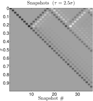
(a)	(b)
(c)	(d)
(e)	(f)

Figure 1: In this figure, we show that the choice of $\tau$ can have a large influence on the localization properties of the orthogonalized snapshots and the quality of the inversion. (a) The primary snapshots $u_{k}$ for the velocity model illustrated in (c); (b) the orthogonalized primary snapshots $\overline{u}_{j}$ generated by Algorithm 1 (converted to the spatial coordinate $x$); (c) the true velocity model (solid, black line) and inversion results for $\tau=2.5\sigma$ — the blue circles are approximately located at ${\widetilde{x}}^{-1}\left({\widetilde{x}}_{j}^{0}\right)$ and the green squares are approximately located at ${\widetilde{x}}^{-1}\left(\widehat{{\widetilde{x}}}_{j}^{0}\right)$. (d) The true velocity model and inversion results when $\tau=3.5\sigma$; (e) the primary snapshots for the velocity model in (d); (f) the orthogonalized primary snapshots for the velocity model in (d).

In Figure 2, we plot the primary snapshots, orthogonalized primary snapshots, and inversion results for two additional velocity models. The first velocity model is illustrated in by the solid, black line in Figure 2(c). We chose $\tau=\sigma$ for this simulation. The orthogonalized snapshots in Figure 2(b) are quite localized. In this case, $\mathrm{cond}(U^{*}U)\approx 4.11\times 10^{3}$.

The second velocity model, illustrated in Figure 2, consists of two smooth inclusions and a discontinuous inclusion. We chose $\tau=1.5\sigma$, which gives $\mathrm{cond}(U^{*}U)\approx 28.10$.

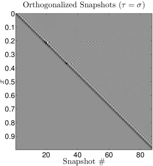
(a)	(b)
(c)	(d)
(e)	(f)

Figure 2: (a) The primary snapshots for the velocity model in (c); (b) the orthogonalized primary snapshots for the velocity model in (c); (c) the velocity model is drawn as a solid, black line, while the inversion results for $\tau=\sigma$ are represented by the blue circles (${\widetilde{x}}^{-1}\left({\widetilde{x}}_{j}^{0}\right)$) and green squares (${\widetilde{x}}^{-1}\left(\widehat{{\widetilde{x}}}_{j}^{0}\right)$). (d) Another velocity model and inversion results; (e) the primary snapshots for the velocity model in (d); (f) the primary orthogonalized snapshots for the velocity model in (d).

Finally, we justify our use of the centers of mass of the reference squared orthogonalized snapshots for the grid points in (5.3) instead of the centers of mass of the squared orthogonalized snapshots for the true medium (which are unknown in practice). In Figure 3, the blue squares represent the true centers of mass of the primary squared orthogonalized snapshots, i.e., the height of the $j\textsuperscript{th}$ blue square is

$${\widetilde{x}}^{-1}\left(\widehat{\gamma}_{j}\int_{0}^{\widetilde{x}_{\max}}\left[\overline{u}_{j}({\widetilde{x}})\right]^{2}\dfrac{1}{\widetilde{v}({\widetilde{x}})}\,d{\widetilde{x}}\right)=\widehat{\gamma}_{j}\int_{0}^{x_{\max}}\left[\overline{u}_{j}(x)\right]^{2}\dfrac{1}{v(x)^{2}}\,dx.$$ (6.1)

The green circles represent the centers of mass of the primary squared orthogonalized snapshots for the (uniform) reference medium, i.e., the height of the $j\textsuperscript{th}$ green circle is

$${\widetilde{x}}^{-1}\left(\widehat{\gamma}_{j}^{0}\int_{0}^{\widetilde{x}_{\max}^{0}}\left[\overline{u}^{0}_{j}({\widetilde{x}}^{0})\right]^{2}\dfrac{1}{\widetilde{v}^{0}({\widetilde{x}}^{0})}\,d{\widetilde{x}}^{0}\right)=\widehat{\gamma}_{j}^{0}\int_{0}^{x_{\max}}\left[\overline{u}^{0}_{j}(x)\right]^{2}\dfrac{1}{v^{0}(x)^{2}}\,dx.$$ (6.2)

In practice, the map ${\widetilde{x}}^{-1}$ cannot be computed exactly since $\widetilde{v}$ is not known a priori. The red asterisks in Figure 3 represent the centers of mass of the reference squared orthogonalized snapshots that are approximately converted to true coordinates using our imaged velocity from (5.4) and a Riemann sum approximation of the integral in (5.5), namely the formulas from (5.6); these are the grid points used in the inversion scheme (and are those shown in Figures 1(c) and (d) and Figures 2(c) and (d)). In particular, Figure 3(a) corresponds to the velocity model in Figure 1(c), Figure 3(b) corresponds to the velocity model in Figure 1(d), Figure 3(c) corresponds to the velocity model in Figure 2(c), and Figure 3(d) corresponds to the velocity model in Figure 2(d). We note that the centers of mass agree quite well (to within a few percent or less) if $\tau$ is chosen appropriately (as in Figures 3(a), (b), and (d)), while they differ significantly (around $28$%) if $\tau$ is chosen poorly (Figure 3(b)). There are even certain choices of $\tau$ for the velocity model in Figure 3(b) for which the grid points are not monotonically increasing — in particular, the orthogonal snapshots have large values far away from the peak centered near the “optimal” grid point, which leads to a poor approximation of the true center of mass.

(a)	(b)
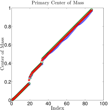
(c)	(d)

Figure 3: In this figure, we plot the centers of mass and approximate centers of mass for (a) the velocity model from Figure 1(c); (b) the velocity model from Figure 1(d) — the disagreement between the various centers of mass in this figure arises because the orthogonalized snapshots are not well localized (because we chose $\tau$ to be too large — see Figure 1(d)–(f)); (c) the velocity model from Figure 2(c); (d) the velocity model from Figure 2(d).

7 Extension to two dimensions

In this section, we extend our results to two dimensions. Because the majority of the results from the one-dimensional case carry over without significant modifications, we will keep our discussion relatively brief.

7.1 Multi-input/multi-output formulation

We begin by defining the region $\Omega\equiv[0,x_{\max}]\times[-y_{\max},y_{\max}]$, where we typically take $y_{\max}=\infty$. We place $m$ sources at the points $(0,y^{i})$ for $i=1,\ldots,m$, which leads us to consider the following Cauchy problem on $\Omega\times[0,\infty[$:

$$A\widehat{u}^{i}+\widehat{u}^{i}_{tt}=0,\qquad\widehat{u}|_{t=0}=\widetilde{q}(A)\delta(x+0)\delta(y-y^{i}),\ \widehat{u}^{i}_{t}|_{t=0}=0,$$ (7.1)

where we take $\widetilde{q}$ is as in (2.8), and

$$A\equiv-v^{2}\left(\frac{\partial^{2}}{\partial x^{2}}+\frac{\partial^{2}}{\partial y^{2}}\right)$$ (7.2)

together with the boundary conditions

$$\widehat{u}^{i}|_{y=\pm y_{\max}}=0,\quad\widehat{u}^{i}_{x}|_{x=0}=0,\ \widehat{u}^{i}|_{x=x_{\max}}=0.$$

We assume $v(0,y)=v(0,0)$ for $y\in[-y_{\max},y_{\max}]$.

For simplicity, we place the receivers at the same locations as the sources. Then, for $k=0,\ldots,2n-1$, we organize our measurements in a matrix $\bm{\mathrm{F}}_{k}\in\mathbb{R}^{m\times m}$ with $F_{k}^{ij}\equiv\widehat{u}^{i}(0,y^{j},k\tau)$. This is the square multi-input/multi-output (square MIMO) problem in control theory terminology.

7.2 MIMO reduced-order model in block form

For $i=1,\ldots,m$, let $u^{i}$ be the solution to the following Cauchy problem on $\Omega\times[0,\infty[$:

$$Au^{i}+u^{i}_{tt}=0,\qquad u^{i}|_{t=0}=b^{i},\ u^{i}_{t}|_{t=0}=0,$$ (7.3)

where

$$b^{i}(x,y)\equiv v(0,0)\widetilde{q}(A)^{1/2}\delta(x+0)\delta(y-y^{i}).$$ (7.4)

For $k=0,\ldots,2n-1$, we define the snapshots

$$U_{k}\equiv\left[u_{k}^{1},\ldots,u_{k}^{m}\right]=T_{k}(P)B,$$ (7.5)

where $P=\cos\left(\tau\sqrt{A}\right)$ is the propagation operator, $B=\left[b^{1},\ldots,b^{m}\right]$, and

$$u_{k}^{i}\equiv u^{i}(x,y,k\tau)=T_{k}(P)b^{i}.$$

Then the measurement matrix

$$\bm{\mathrm{F}}_{k}=U_{0}^{*}U_{k}=B^{*}T_{k}(P)B,$$ (7.6)

where ^∗ is defined as before (see (3.11)) with the inner product

$$\left\llangle u,w\right\rrangle\equiv\int_{\Omega}u(x,y)w(x,y)\frac{1}{v^{2}(x,y)}\,dx\,dy.$$

The measurement matrix can also be represented by

$$\bm{\mathrm{F}}_{k}=\int_{-1}^{1}T_{k}(\mu)\bm{\mathrm{\eta}}_{0}(\mu)\,d\mu,$$ (7.7)

where $\bm{\mathrm{\eta}}_{0}$ is an $m\times m$ matrix measure. In particular, $\eta^{ij}_{0}(\mu)=\eta^{i}(0,y^{j},\mu)$ where $\eta^{i}(x,y,\mu)$ is defined as in (3.3) with $\rho$ replaced by

$$\rho^{i}(x,y,\lambda)\equiv\displaystyle\sum_{l=1}^{\infty}\delta(\lambda-\lambda_{l})\frac{z_{l}(0,y^{i})}{v(0,0)^{2}}z_{l}(x,y);$$ (7.8)

$(\lambda_{l},z_{l})$ are eigenpairs of $A$ with $\left\llangle z_{l},z_{j}\right\rrangle=\delta_{lj}$. Next we construct a generalized Gaussian quadrature such that

$$\int_{-1}^{1}T_{k}(\mu)\bm{\mathrm{\eta}}_{0}(\mu)\,d\mu=\sum_{j=1}^{n}\bm{\mathrm{Y}}_{j}T_{k}(\bm{\mathrm{\Theta}}_{j})\bm{\mathrm{Y}}_{j}^{T}=\bm{\mathrm{F}}_{k}\quad\text{for }k=0,\ldots,2n-1,$$ (7.9)

where $\bm{\mathrm{Y}}_{j}=\left[\bm{\mathrm{\Psi}}_{1j},\ldots,\bm{\mathrm{\Psi}}_{mj}\right]\in\mathbb{R}^{m\times m}$, i.e., for $l=1,\ldots,m$, $\bm{\mathrm{\Psi}}_{lj}\in\mathbb{R}^{m}$ is the $l\textsuperscript{th}$ column of the matrix $\bm{\mathrm{Y}}_{j}$, and $\bm{\mathrm{\Theta}}_{j}=\mathrm{diag\ }(\theta_{1j},\ldots,\theta_{mj})\in\mathbb{R}^{m\times m}$.

We define the snapshot matrix $U=\left[U_{1},\ldots,U_{n}\right]$. Then matrix versions of Lemmas 4.2–4.4 hold. In particular, if

$$\bm{\mathrm{H}}=(U^{*}U)^{-1}(U^{*}PU)\in\mathbb{R}^{mn\times mn}\quad\text{and}\quad\bm{\mathrm{E}}_{1}=\begin{bmatrix}\bm{\mathrm{I}}_{m\times m}\\ \bm{\mathrm{0}}_{m\times m}\\ \vdots\\ \bm{\mathrm{0}}_{m\times m}\end{bmatrix}\in\mathbb{R}^{mn\times m},$$

then

$$\bm{\mathrm{F}}_{k}=\bm{\mathrm{E}}_{1}^{T}(U^{*}U)T_{k}(\bm{\mathrm{H}})\bm{\mathrm{E}}_{1}.$$ (7.10)

Additionally, $\bm{\mathrm{H}}$ has the eigendecomposition

$$\bm{\mathrm{H}}=\bm{\mathrm{\Phi}}\bm{\mathrm{\Theta}}\bm{\mathrm{\Phi}}^{T}U^{*}U,$$ (7.11)

where $\bm{\mathrm{\Theta}}$, $\bm{\mathrm{\Phi}}\in\mathbb{R}^{mn\times mn}$ such that $\bm{\mathrm{\Phi}}^{T}U^{*}U\bm{\mathrm{\Phi}}=\bm{\mathrm{I}}_{mn\times mn}$. We emphasize $\bm{\mathrm{H}}$ is known by the matrix version of Lemma 4.4 (with $f_{k}$ replaced by $\bm{\mathrm{F}}_{k}$ in the statement and proof of the lemma). Substituting (7.11) into (7.10) gives

$$\bm{\mathrm{F}}_{k}=\bm{\mathrm{\chi}}^{T}T_{k}(\bm{\mathrm{\Theta}})\bm{\mathrm{\chi}}\quad\text{for }k=0,\ldots,2n-1,\quad\text{where}\quad\bm{\mathrm{\chi}}\equiv\bm{\mathrm{\Phi}}^{T}U^{*}U\bm{\mathrm{E}}_{1}\in\mathbb{R}^{mn\times m}.$$ (7.12)

Comparing this with (7.9) gives

$$\mathrm{diag\ }\ \bm{\mathrm{\Theta}}_{j}=\bm{\mathrm{\Theta}}\quad\text{and}\quad\bm{\mathrm{\chi}}=\begin{bmatrix}\bm{\mathrm{Y}}_{1}^{T}\\ \vdots\\ \bm{\mathrm{Y}}_{n}^{T}\end{bmatrix}.$$ (7.13)

We may also construct a symmetric, positive-semidefinite matrix $\bm{\mathrm{C}}\in\mathbb{R}^{m\times m}$ and a symmetric, block-tridiagonal matrix

$$\bm{\mathrm{P}}_{n}=\begin{bmatrix}\bm{\mathrm{\alpha}}_{1}&\bm{\mathrm{\beta}}_{1}^{T}&&\\ \bm{\mathrm{\beta}}_{1}&\bm{\mathrm{\alpha}}_{2}&\ddots&\\ &\ddots&\ddots&\bm{\mathrm{\beta}}_{n-1}^{T}\\ &&\bm{\mathrm{\beta}}_{n-1}&\bm{\mathrm{\alpha}}_{n}\end{bmatrix}=\bm{\mathrm{P}}_{n}^{T}\in\mathbb{R}^{mn\times mn}$$ (7.14)

with $\bm{\mathrm{\alpha}}_{j}=\bm{\mathrm{\alpha}}_{j}^{T}\in\mathbb{R}^{m\times m}$ and $\bm{\mathrm{\beta}}_{j}\in\mathbb{R}^{m\times m}$ such that

$$\bm{\mathrm{F}}_{k}=\displaystyle\sum_{j=1}^{n}\bm{\mathrm{Y}}_{j}T_{k}(\bm{\mathrm{\Theta}}_{j})\bm{\mathrm{Y}}_{l}^{T}=\bm{\mathrm{C}}^{1/2}\bm{\mathrm{E}}_{1}^{T}T_{k}(\bm{\mathrm{P}}_{n})\bm{\mathrm{E}}_{1}\bm{\mathrm{C}}^{1/2}\quad\text{for }k=0,\ldots,2n-1.$$ (7.15)

Taking $k=0$ in (7.15) gives

$$\bm{\mathrm{C}}=\displaystyle\sum_{j=1}^{n}\bm{\mathrm{Y}}_{j}\bm{\mathrm{Y}}_{j}^{T}=\bm{\mathrm{F}}_{0}=\int_{-1}^{1}\bm{\mathrm{\eta}}_{0}(\mu)\,d\mu.$$ (7.16)

From (7.16), we immediately see that $\bm{\mathrm{C}}$ is symmetric and positive-semidefinite — $\bm{\mathrm{C}}$ will be positive-definite if and only if the matrix $\left[\bm{\mathrm{Y}}_{1},\ldots,\bm{\mathrm{Y}}_{n}\right]=\left[\bm{\mathrm{\Psi}}_{11},\ldots,\bm{\mathrm{\Psi}}_{mn}\right]\in\mathbb{R}^{m\times mn}$ has rank equal to $m$.

Analogously to the 1D case, the matrix $\bm{\mathrm{P}}_{n}$ has the eigendecomposition

$$\bm{\mathrm{P}}_{n}\bm{\mathrm{X}}=\bm{\mathrm{X}}\bm{\mathrm{\Theta}},\quad\bm{\mathrm{X}}=\left[\bm{\mathrm{X}}_{1},\ldots,\bm{\mathrm{X}}_{n}\right]\in\mathbb{R}^{mn\times mn},\quad\bm{\mathrm{X}}_{l}^{T}\bm{\mathrm{X}}_{j}=\delta_{lj}\bm{\mathrm{I}}_{m\times m}$$ (7.17)

(the matrices $\bm{\mathrm{X}}_{j}\in\mathbb{R}^{m\times m}$ are “block eigenvectors” of $\bm{\mathrm{P}}_{n}$ corresponding to the “block eigenvalues” $\bm{\mathrm{\Theta}}_{j}$).

We compare (7.15) with (7.12)–(7.13) to find $\bm{\mathrm{E}}_{1}^{T}\bm{\mathrm{X}}_{j}=\bm{\mathrm{C}}^{-1/2}\bm{\mathrm{Y}}_{j}$. Because (7.17) is equivalent to $\bm{\mathrm{\Theta}}\bm{\mathrm{X}}^{T}=\bm{\mathrm{X}}^{T}\bm{\mathrm{P}}_{n}$, the matrix $\bm{\mathrm{P}}_{n}$ may be constructed using the block-Lanczos algorithm in Algorithm 1 (the $mn\times m$ Lanczos “vectors” $\bm{\mathrm{Q}}_{j}$ in this algorithm are the “columns” of the matrix $\bm{\mathrm{X}}^{T}$, i.e., $\bm{\mathrm{X}}^{T}=\left[\bm{\mathrm{Q}}_{1},\ldots,\bm{\mathrm{Q}}_{n}\right]$) — see, e.g., the book by Parlett [40].

Algorithm 1 Block Lanczos Algorithm for Computing $\bm{\mathrm{\alpha}}_{j}$, $\bm{\mathrm{\beta}}_{j}$.

$\bm{\mathrm{C}}$, $\bm{\mathrm{\Theta}}_{j}$, $\bm{\mathrm{Y}}_{j}$ for $j=1,\ldots,n$

$\bm{\mathrm{\alpha}}_{j}$ ($j=1,\ldots,n$) and $\bm{\mathrm{\beta}}_{j}$ ($j=1,\ldots,n-1$), i.e., the nonzero elements of $\bm{\mathrm{P}}_{n}$

Set $\bm{\mathrm{Q}}_{0}=\bm{\mathrm{0}}_{mn\times m}$ and

$$\bm{\mathrm{Q}}_{1}=\begin{bmatrix}\bm{\mathrm{Y}}_{1}^{T}\bm{\mathrm{C}}^{-1/2}\\ \vdots\\ \bm{\mathrm{Y}}_{n}^{T}\bm{\mathrm{C}}^{-1/2}\end{bmatrix}.$$

for $j=1,\ldots,n$ do

1. $\bm{\mathrm{\alpha}}_{j}=\bm{\mathrm{Q}}_{j}^{T}\bm{\mathrm{\Theta}}\bm{\mathrm{Q}}_{j}$;

2. $\bm{\mathrm{R}}_{j}=\bm{\mathrm{\Theta}}\bm{\mathrm{Q}}_{j}-\bm{\mathrm{Q}}_{j-1}\bm{\mathrm{\beta}}_{j-1}^{T}-\bm{\mathrm{Q}}_{j}\bm{\mathrm{\alpha}}_{j}$;

3. $\bm{\mathrm{\beta}}_{j}=\left(\bm{\mathrm{R}}_{j}^{T}\bm{\mathrm{R}}_{j}\right)^{1/2}$;

4. $\bm{\mathrm{Q}}_{j+1}=\bm{\mathrm{R}}_{j}\bm{\mathrm{\beta}}_{j}^{-1}$.

end for

7.3 Continuum interpretation in two dimensions

We now derive an inversion algorithm analogous to the algorithm we constructed in § 5. The key ingredients are the matrix extensions of $\widehat{\gamma}_{j}$ and $\gamma_{j}$; in particular, we now consider $m\times m$ symmetric, positive-definite matrices $\widehat{\bm{\mathrm{\Gamma}}}_{j}$, $\bm{\mathrm{\Gamma}}_{j}$ for $j=1,\ldots,n$. These matrices may be computed via Algorithm 2 [15, 20], which is a matrix version of Algorithm 2. We conjecture that full rank of the Gram matrix $U^{*}U$ is a sufficient condition for Algorithm 2 to succeed.

Algorithm 2 Computation of $\widehat{\bm{\mathrm{\Gamma}}}_{j}$, $\bm{\mathrm{\Gamma}}_{j}$

$\bm{\mathrm{C}}$, $\bm{\mathrm{Y}}_{l}$, $\bm{\mathrm{\Lambda}}_{l}=-\xi(\bm{\mathrm{\Theta}}_{l})\in\mathbb{R}^{m\times m}$ for $l=1,\ldots,n$

$\widehat{\bm{\mathrm{\Gamma}}}_{j}$, $\bm{\mathrm{\Gamma}}_{j}$, $j=1,\ldots,n$

Set $\overline{\bm{\mathrm{\omega}}}_{0}=\bm{\mathrm{0}}_{2mn\times m}$, $\overline{\bm{\mathrm{\mu}}}_{1}=\sqrt{0.5}\cdot\left[\bm{\mathrm{Y}}_{1},\bm{\mathrm{Y}}_{1},\bm{\mathrm{Y}}_{2},\bm{\mathrm{Y}}_{2},\ldots,\bm{\mathrm{Y}}_{n},\bm{\mathrm{Y}}_{n}\right]^{T}\in\mathbb{R}^{2mn\times m}$, and
$\bm{\mathrm{L}}=\mathrm{diag\ }\ \left(\bm{\mathrm{\Lambda}}_{1}^{1/2},-\bm{\mathrm{\Lambda}}_{1}^{1/2},\bm{\mathrm{\Lambda}}_{2}^{1/2},-\bm{\mathrm{\Lambda}}_{2}^{1/2},\ldots,\bm{\mathrm{\Lambda}}_{n}^{1/2},-\bm{\mathrm{\Lambda}}_{n}^{1/2}\right)\in\mathbb{R}^{2mn\times 2mn}$.

for $j=1,\ldots,n$ do

1. $\widehat{\bm{\mathrm{\Gamma}}}_{j}=\left(\overline{\bm{\mathrm{\mu}}}_{j}^{T}\overline{\bm{\mathrm{\mu}}}_{j}\right)^{-1}$;

2. $\overline{\bm{\mathrm{\omega}}}_{j}=\overline{\bm{\mathrm{\omega}}}_{j-1}+\bm{\mathrm{L}}\overline{\bm{\mathrm{\mu}}}_{j}\widehat{\bm{\mathrm{\Gamma}}}_{j}$;

3. $\bm{\mathrm{\Gamma}}_{j}=\left(\overline{\bm{\mathrm{\omega}}}_{j}^{T}\overline{\bm{\mathrm{\omega}}}_{j}\right)^{-1}$;

4. $\overline{\bm{\mathrm{\mu}}}_{j+1}=\overline{\bm{\mathrm{\mu}}}_{j}-\bm{\mathrm{L}}\overline{\bm{\mathrm{\omega}}}_{j}\bm{\mathrm{\Gamma}}_{j}$.

end for

Remark 7.1.

In what follows, we illustrate one way in which the inversion algorithm from § 5 may be extended to 2D. In particular, we avoid technical details and focus on providing an heuristic justification of our algorithm. We have recently developed a more rigorous 2D inversion algorithm [37] that relies on many of the ideas discussed in the present paper.

In 2D, an invertible coordinate transformation to slowness (also known as ray or traveltime) coordinates analogous to (2.2) may not exist for most relevant cases due to the formation of caustics [42]. If the medium under consideration is “approximately layered” in the vertical direction, however, it is plausible that an invertible transformation to ray coordinates exists.

Henceforth we assume that rays perpendicular to the line $x=0$ do not intersect. This ensures that the ray coordinate transformation $(x,y)\mapsto(\zeta,\nu)$ exists and is invertible. Here $\zeta$ represents the traveltime along a ray and $\nu$ is orthogonal to $\zeta$; we also assume the line $x=0$ is mapped to the line $\zeta=0$. Thus the curves $\nu=\mathrm{const.\ }$ represent the rays orthogonal to the line $x=0$. We define ${\widetilde{u}}^{i}(\zeta,\nu)\equiv u^{i}(x(\zeta,\nu),y(\zeta,\nu))$ (and similarly for other functions of $x$ and $y$). Then (7.3) transforms to

$$\widetilde{A}{\widetilde{u}}^{i}+{\widetilde{u}}^{i}_{tt}=0,\qquad{\widetilde{u}}|_{t=0}=\widetilde{b},\ {\widetilde{u}}_{t}|_{t=0}=0,$$ (7.18)

where $\widetilde{A}$ is the operator $A$ represented in ray coordinates [42]. In particular, in an “approximately layered” medium, we approximate $\widetilde{A}$ along rays by

$$\widetilde{A}\approx-\widetilde{v}\frac{\partial}{\partial\zeta}\left(\frac{1}{\widetilde{v}}\frac{\partial{\widetilde{u}}}{\partial\zeta}\right);$$ (7.19)

thus our problem essentially reduces to a 1D problem (in a layered medium, we have $\nu=y$ and $\zeta=\int_{0}^{x}1/v(x^{\prime})\,dx^{\prime}$, as in 1D).

As in the 1D setting, we consider the first $n$ primary and dual snapshots, namely $\widetilde{U}_{k}$ and $\widetilde{W}_{k}$, respectively ($k=0,\ldots,n-1$). The orthogonalized snapshots $\overline{U}_{j}$ and $\overline{W}_{j}$ (computed via an algorithm analogous to Algorithm 1) will again be localized in some sense. Moreover, we have $\widehat{\bm{\mathrm{\Gamma}}}_{j}=(\overline{U}_{j}^{*}\overline{U}_{j})^{-1}$ and $\bm{\mathrm{\Gamma}}_{j}=(\overline{W}_{j}^{*}\overline{W}_{j})^{-1}$ (where ^∗ is defined as in § 4.1 with respect to an appropriate inner product), so $\widehat{\bm{\mathrm{\Gamma}}}_{j}$ and $\bm{\mathrm{\Gamma}}_{j}$ are symmetric, positive-semidefinite matrices. The matrices $\widehat{\bm{\mathrm{\Gamma}}}_{j}$, $\bm{\mathrm{\Gamma}}_{j}$ may be loosely interpreted to contain information about the local wave speed as follows.

As in [15, 20], we use the diagonals of $\widehat{\bm{\mathrm{\Gamma}}}_{j}^{-1}$ and $\bm{\mathrm{\Gamma}}_{j}$, denoted by $\widehat{\bm{\mathrm{\gamma}}}_{j}\in\mathbb{R}^{m}$ and $\bm{\mathrm{\gamma}}_{j}\in\mathbb{R}^{m}$, respectively, as the analogues of $\widehat{\gamma}_{j}$ and $\gamma_{j}$ from (5.4). The reasoning behind our use of the diagonals is twofold. First, the set of data matrices $\bm{\mathrm{F}}_{k}$ ($k=0,\ldots,2n-1$) is effectively three-dimensional, as is the set of $\widehat{\bm{\mathrm{\Gamma}}}_{j}$, $\bm{\mathrm{\Gamma}}_{j}$. Our problem is overdetermined because we are trying to recover an approximation of $v$ on a two-dimensional grid. Although we use the full data to compute $\widehat{\bm{\mathrm{\Gamma}}}_{j}$ and $\widehat{\bm{\mathrm{\Gamma}}}$, we reduce the dimensionality by using only the diagonals $\widehat{\bm{\mathrm{\gamma}}}_{j}$ and $\bm{\mathrm{\gamma}}_{j}$ [20]. Second, recall $\widehat{\bm{\mathrm{\Gamma}}}_{j}^{-1}=(\overline{U}_{j}^{*}\overline{U}_{j})$. Then $\bm{\mathrm{e}}_{i}^{T}\bm{\mathrm{\widehat{\gamma}}}_{j}=\widehat{\Gamma}^{-1}_{j,ii}=\left(\overline{U}_{j}^{i}\right)^{*}\overline{U}_{j}^{i}$. Since the approximate operator $\widetilde{A}$ in (7.19) is of the same form as in the 1D case (see (3.14)), it seems reasonable to assume the quantities $\bm{\mathrm{e}}_{i}^{T}\widehat{\bm{\mathrm{\gamma}}}_{j}$ are related to localized averages of $\frac{1}{\widetilde{v}}$.

Our algorithm thus proceeds as follows. We consider a background velocity $v^{0}$ with $v^{0}(0,y)=v(0,0)$ for $y\in[-y_{\max},y_{\max}]$. We choose the velocity to be simple enough so the ray coordinate transformation is well-posed; for example, we took $v^{0}=v(0,0)$ in our numerical experiments. For a constant background velocity, ray coordinates are particularly simple — in fact, $\zeta=\frac{1}{v_{0}}x$ and $\nu=y$.

The grid points at which we approximate the true velocity are $(\zeta^{0}_{j},\nu^{0}_{i})$ and $(\widehat{\zeta}^{0}_{j},\widehat{\nu}^{0}_{i})$, where, for a constant background velocity $v^{0}$, $\zeta^{0}_{j}$ is computed as in the 1D case and $\nu^{0}_{i}=y^{i}$. The dual grid points $(\widehat{\zeta}^{0}_{j},\widehat{\nu}^{0}_{i})$ are defined in a similar manner. The velocity is approximated at the grid points (in ray coordinates) by

$$\widetilde{v}(\zeta^{0}_{j},\nu^{0}_{i})\approx\widetilde{v}^{0}(\zeta^{0}_{j},\nu^{0}_{i})\frac{\bm{\mathrm{e}}_{i}^{T}\widehat{\bm{\mathrm{\gamma}}}^{0}_{j}}{\bm{\mathrm{e}}_{i}^{T}\widehat{\bm{\mathrm{\gamma}}}_{j}}.\quad\text{and}\quad\widetilde{v}(\widehat{\zeta}^{0}_{j},\widehat{\nu}^{0}_{i})\approx\widetilde{v}^{0}(\widehat{\zeta}^{0}_{j},\widehat{\nu}^{0}_{i})\frac{\bm{\mathrm{e}}_{i}^{T}\bm{\mathrm{\gamma}}_{j}}{\bm{\mathrm{e}}_{i}^{T}\bm{\mathrm{\gamma}}^{0}_{j}}.$$ (7.20)

We may approximately convert the grid points $(\zeta^{0}_{j},\nu^{0}_{i})$ and $(\widehat{\zeta}^{0}_{j},\widehat{\nu}^{0}_{i})$ to spatial coordinates $(x^{0}_{j},y^{0}_{i})$ and $(\widehat{x}^{0}_{j},\widehat{y}^{0}_{i})$, respectively, by inverting the coordinate transform using our imaged velocity (much like in the 1D case).

In Figure 4, we plot the results of two numerical experiments using our 2D inversion method. In both cases, we used a constant background velocity. Figure 4(a) is the image of a block — the true velocity corresponding to Figure 4(a) is plotted in Figure 4(b); Figure 4(c) is the image of a dipping interface — the true velocity corresponding to Figure 4(c) is plotted in Figure 4(d). In Figures 4(a) and (c), the horizontal axis is in slowness coordinates, while in Figures 4(b) and (d) the horizontal axis is in physical coordinates. They show qualitatively correct inversion results, even though our assumption on nonintersecting rays fails for the block model.

The above imaging procedure was further improved of by some of the authors with preliminary results (including imaging of a 2D Marmousi cross-section) reported in [37].

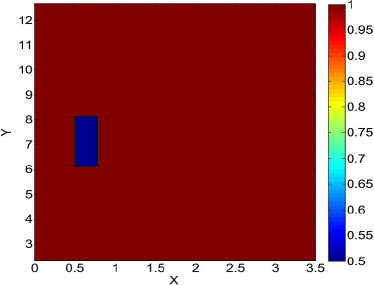
(a)	(b)

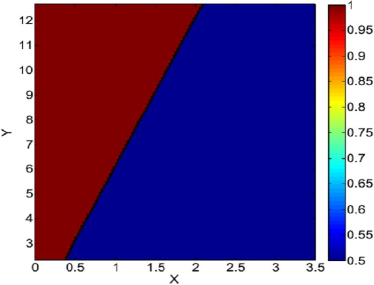
Figure 4: In this figure, we plot the results of two numerical experiments using our 2D inversion method sketched in this section. The horizontal axis is in slowness coordinates for figures (a) and (c) while it is in true (physical) coordinates for figures (b) and (d). We used a constant background velocity in both experiments: (a) image of a block inclusion; (b) true velocity corresponding to (a); (c) image of a dipping interface; (d) true velocity corresponding to (d).

8 Conclusion

We developed a model reduction framework for the solution of inverse hyperbolic problems. This is a brief summary of our approach.

• We start with a one-dimensional problem and single-input/single output (SISO) time-domain boundary measurements.

  • We sample the data on a given temporal interval consistent with the Nyquist-Shannon theorem and construct the ROM interpolating the data at the sampling points. The ROM is obtained via the Chebyshev moment problem, which can be equivalently represented via Galerkin projection on the subspace of the wavefield snapshots, i.e., a Krylov subspace of the propagation operator.

  • Using the Lanczos algorithm, we transform the projected system to a sparse form that mimics a finite-difference discretization of the underlying wave problem. This transformation is equivalent to Gram–Schmidt orthogonalization, and yields a localized orthogonal basis on the snapshot subspace.

  • We estimate the unknown PDE coefficient via coefficients of the sparse system. The coefficients of this sparse system are weighted averages of the true, unknown velocity, where the weight functions are localized (in particular, they are the squared orthogonalized snapshots).

  • Numerical experiments show quantitatively good images of layered media, though the image quality depends on the consistency between the time-sampling and the pulse spectral content.

• We outline a generalization to the multidimensional setting (on a 2D example) with square multi-input/multi-output (MIMO) boundary data.

  • We construct the MIMO ROM data via the block-counterpart of the SISO algorithm.

  • The continuum interpretation of the MIMO ROM is done via geometrical optics.

  • Two-dimensional numerical experiments show that the imaging algorithm gives qualitatively correct results even when the geometric optics assumption does not hold.

The key of the efficiency of the proposed approach is the weak dependence of the orthogonalized snapshots on the media, which allows us to use a single background Krylov basis for accurate Galerkin projection. At the moment we only have experimental verification of that phenomenon, and can conjecture a result similar to the asymptotic independence of the optimal grids on variable coefficients [5]. We believe that such a basis can also be found for interpolatory model reduction in the frequency domain (via a rational Krylov subspace), and investigation in this direction is under way.

Another advantage of our proposed algorithm over traditional FWI is that modeling errors are not an issue; because we use a homogeneous background wavespeed, the background solution can be obtained analytically. We should mention, however, that our algorithm does not perform well if a nonconstant background wavespeed that is not very close to the true wavespeed is used. Although this limits the ability of our algorithm to be used iteratively, we believe our algorithm performs very well either as a direct algorithm or as a nonlinear preconditioner for generating an initial model for FWI [10]. Additionally, in § 6, we discussed the stability of the 1D algorithm in the context of the choice of the sampling stepsize $\tau$, which essentially plays the role of a regularization parameter.

We must admit that the generalization to multidimensional problems is still in its initial stage. The square MIMO formulation is overdetermined; this gives rise to a multitude of different imaging formulas, even though the equivalent state-variable ROM representation is unique up to a change of basis. One such formula, outlined in [37] (still based on the MIMO ROM construction presented in this paper), apparently has sharper resolution than the algorithm of § 7.3. We also discovered some stability issues in the 2D case — these will be addressed in a forthcoming work.

Moreover, the collocated square MIMO formulation considered in this work may not be suitable for some practically important measurement systems in seismic exploration and other remote sensing applications. To circumvent this deficiency, we are looking at the extension of our approach to non-collocated source-receiver arrays with a different number of sources and receivers, which leads to rectangular MIMO formulations within the Galerkin–Petrov projection framework. Another possible extension is a back-scattering formulation used for radar imaging, corresponding to one or a few diagonals of the square MIMO matrix data set.

Appendix A Proofs

In this appendix, we present some calculations and proofs we omitted in the body of the paper.

A.1 Derivation of (3.2)

We begin by recalling (2.12):

$$\widehat{u}(x,k\tau)=2\int_{0}^{\infty}\cos(k\tau s)\rho(x,s^{2})s\widetilde{q}(s^{2})\,ds.$$ (A.1)

We make the change of variables $y=\tau s$ in (A.1) to obtain

$$\widehat{u}(x,k\tau)=\frac{2}{\tau^{2}}\int_{0}^{\infty}\cos(ky)\rho(x,(y/\tau)^{2})y\widetilde{q}\left((y/\tau)^{2}\right)\,dy.$$ (A.2)

Henceforth we will take the principal branch of $\arccos$, namely $\arccos:[-1,1]\mapsto[0,\pi]$.

Next, we break the integral in (A.2) into infinitely many segments so we can apply an invertible change of coordinates of the form $\mu=\cos y$ to each segment; in particular, we have

$$\widehat{u}(x,k\tau)=\frac{2}{\tau^{2}}\displaystyle\sum_{j=0}^{\infty}\int_{2j\pi}^{(2j+1)\pi}\cos(ky)\rho\left(x,(y/\tau)^{2}\right)y\widetilde{q}\left((y/\tau)^{2}\right)\,dy\\ +\frac{2}{\tau^{2}}\displaystyle\sum_{j=1}^{\infty}\int_{(2j-1)\pi}^{2j\pi}\cos(ky)\rho\left(x,(y/\tau)^{2}\right)y\widetilde{q}\left((y/\tau)^{2}\right)\,dy.$$ (A.3)

We now make the following changes of variables in the first and second integrals in (A.3), respectively:

$$\mu=\cos(y),\quad y=\arccos(\mu)+2j\pi,\quad dy=-\frac{1}{\sqrt{1-\mu^{2}}}d\mu;$$ (A.4a)

$$\nu=\cos(y),\quad y=-\arccos(\nu)+2j\pi,\quad dy=\frac{1}{\sqrt{1-\nu^{2}}}d\nu.$$ (A.4b)

Using (A.4a) and (A.4b) in the first and second integrals in (A.3), respectively, we obtain

$$\widehat{u}(x,k\tau) =\frac{2}{\tau^{2}}\sum_{j=0}^{\infty}\int_{1}^{-1}\cos(k(\arccos(\mu)+2j\pi))\rho\left(x,\left(\frac{\arccos(\mu)+2j\pi}{\tau}\right)^{2}\right)$$

$$\qquad\cdot(\arccos(\mu)+2j\pi)\widetilde{q}\left(\left(\frac{\arccos(\mu)+2j\pi}{\tau}\right)^{2}\right)\left(-\frac{1}{\sqrt{1-\mu^{2}}}\right)\,d\mu$$

$$+\frac{2}{\tau^{2}}\sum_{j=1}^{\infty}\int_{-1}^{1}\cos(k(-\arccos(\nu)+2j\pi))\rho\left(x,\left(\frac{-\arccos(\nu)+2j\pi}{\tau}\right)^{2}\right)$$

$$\qquad\cdot(-\arccos(\nu)+2j\pi)\widetilde{q}\left(\left(\frac{-\arccos(\nu)+2j\pi}{\tau}\right)^{2}\right)\frac{1}{\sqrt{1-\nu^{2}}}\,d\nu.$$

We then use the $2\pi$-periodicity of cosine, transform $j\rightarrow-j$ in the second sum, and use the definition of the Chebyshev polynomials of the first kind to find

$$\widehat{u}(x,k\tau) =\frac{2}{\tau^{2}}\sum_{j=0}^{\infty}\int_{-1}^{1}T_{k}(\mu)\rho\left(x,\left(\frac{\arccos(\mu)+2j\pi}{\tau}\right)^{2}\right)$$

$$\qquad\cdot(\arccos(\mu)+2j\pi)\widetilde{q}\left(\left(\frac{\arccos(\mu)+2j\pi}{\tau}\right)^{2}\right)\frac{1}{\sqrt{1-\mu^{2}}}\,d\mu$$

$$-\frac{2}{\tau^{2}}\sum_{j=-\infty}^{-1}\int_{-1}^{1}T_{k}(\mu)\rho\left(x,\left(\frac{\arccos(\mu)+2j\pi}{\tau}\right)^{2}\right)$$

$$\qquad\cdot(\arccos(\mu)+2j\pi)\widetilde{q}\left(\left(\frac{\arccos(\mu)+2j\pi}{\tau}\right)^{2}\right)\frac{1}{\sqrt{1-\mu^{2}}}\,d\mu$$

$$=\int_{-1}^{1}T_{k}(\mu)\eta(x,\mu)\,d\mu.$$

A.2 Support of $c^{-1}\eta_{0}(\mu)\,d\mu$ for constant velocity

For $s\in[-1,1]$, let us define $N(s)\equiv\int_{-1}^{s}c^{-1}\eta_{0}(\mu)\,d\mu$. Then the hypothesis of Lemma 4.1 holds if $N$ has at least $n$ points of increase for $s\in[-1,1]$ (the set of all points of increase for $N$ is also known as the support or spectrum of the measure $c^{-1}\eta_{0}(\mu)\,d\mu$ — see, e.g., Chapter 1 of [23]). Here, we show that if the wavespeed is constant, then $N$ has exactly $n$ points of increase in $[-1,1]$; we provide a qualitative explanation for the nonconstant wavespeed case at the end of the section.

Recall from (3.3) and (2.6) that

$$\eta_{0}(\mu)=\eta(0,\mu)=\sum_{j=-\infty}^{\infty}r_{j}(\mu)\sum_{l=1}^{\infty}\delta\left(\frac{(\arccos(\mu)+2\pi j)^{2}}{\tau^{2}}-\lambda_{l}\right)\frac{z_{l}(0)}{v(0)^{2}}z_{l}(x),$$

where $(\lambda_{l},z_{l}(x))$ is the $l^{\textsuperscript{th}}$ eigenpair of $A$ and

$$r_{j}(\mu)\equiv 2\mathrm{sgn}(j)\widetilde{q}\left(\frac{(\arccos(\mu)+2j\pi)^{2}}{\tau^{2}}\right)\frac{\arccos(\mu)+2j\pi}{\tau^{2}}\frac{1}{\sqrt{1-\mu^{2}}}.$$

Note that if $\widetilde{q}$ is given by (2.9), then $r_{j}>0$ for $\mu\in]-1,1[$.

For simplicity, we take the wavespeed $v\equiv 1$ and $x_{\max}=1$. Recall that we take $2n$ measurements on the time interval $[0,T]$ at the discrete times $k\tau$ for $k=0,\ldots,2n-1$, where $(2n-1)\tau=T$. For the sake of illustration, let us take $\tau=1/n$ for some $n$; then $T=2-\frac{1}{n}$ and the timestep $\tau$ is determined by the number of snapshots we wish to take.

When $v\equiv 1$, the eigenfunctions of $A$ satisfy

$$-z_{l,xx}=\lambda_{l}z_{l},\qquad z_{l,x}|_{x=0}=0,\ z_{l}|_{x=1}=0.$$

Then the eigenvalues and (orthonormal) eigenfunctions are

$$\lambda_{l}=\left[\frac{(2l-1)\pi}{2}\right]^{2}\quad\text{and}\quad z_{l}(x)=\sqrt{2}\cos\left(\sqrt{\lambda_{l}}x\right),\quad l=1,2,\ldots.$$ (A.5)

Reversing the arguments from § A.1, using the fact that $\tau=1/n$, and using the expressions in (A.5) for the eigenfunctions of $A$ we find

$$N(s) =4c^{-1}\left[\sum_{j=0}^{\infty}\int_{(\arccos(s)+2\pi j)n}^{(2j+1)\pi n}\widetilde{q}(r^{2})r\sum_{l=1}^{\infty}\delta(r^{2}-\lambda_{l})\,dr\right.$$ (A.6)

$$\left.\qquad+\sum_{j=1}^{\infty}\int_{(2j-1)\pi n}^{(2\pi j-\arccos(s))n}\widetilde{q}(r^{2})r\sum_{l=1}^{\infty}\delta(r^{2}-\lambda_{l})\,dr\right].$$

For a fixed value of $s\in[-1,1]$, only certain values of $\lambda_{l}$ will contribute to the above integrals. In Figure 5, we illustrate the first couple of integration intervals for the first (second) integral in (A.6) in red (blue) for a given value of $s$. The square roots of the eigenvalues from (A.5) are marked with crosses — here $n=6$. As $s\rightarrow 1^{-}$, the intervals will increase in width until the positive half of the real line is covered.

Figure 5: In this figure, we sketch the integration intervals for the integrals in (A.6) for a fixed value of $s\in[-1,1]$. The square roots of the eigenvalues of $A$, namely $\sqrt{\lambda_{l}}$, are marked with crosses. The red intervals in the figure correspond to the first two integration intervals for the first integral (i.e., for $j=0$, $1$) while the blue intervals correspond to the first two integration intervals for the second integral (i.e., for $j=1$, $2$). We took $n=6$ for this figure.

From (A.5), we see that $\sqrt{\lambda_{l}}\in]0,n\pi[$ for $l=1,\ldots,n$. As $s$ increases from $-1$ to $1$ more and more eigenvalues will be caught in the integration intervals for the integrals in (A.6) and contribute to $N(s)$. Since the eigenvalues of $A$ are uniformly distributed on the positive real line when $v$ is constant, each integration interval will contain the same number of eigenvalues as every other integration interval for every value of $s$, and each interval will contain at most $n$ eigenvalues.

For $i=1,\ldots,n$, let $s_{i}\in[-1,1]$ be defined by

$$n\arccos(s_{i})=\sqrt{\lambda_{n-(i-1)}}\Leftrightarrow s_{i}=\cos\left(\frac{\sqrt{\lambda_{n-(i-1)}}}{n}\right).$$

Using this and (A.6) we obtain

$$N(s)=\sum_{i=1}^{n}\alpha_{i}H(s-s_{i}),$$ (A.7)

where $H$ is the Heaviside step function and

$$\alpha_{i}=\sum_{j=0}^{\infty}\widetilde{q}\left(\left(\sqrt{\lambda_{n-(i-1)}}+2\pi nj\right)^{2}\right)\left(\sqrt{\lambda_{n-(i-1)}}+2\pi nj\right)\\ +\sum_{j=1}^{\infty}\widetilde{q}\left(\left(\sqrt{\lambda_{n+i}}+2\pi nj\right)^{2}\right)\left(\sqrt{\lambda_{n+i}}+2\pi nj\right).$$

(For our choice of $\widetilde{q}$ in (2.9), both of the above series converge.) The upshot of (A.7) is that the $n$ points of increase of $N(s)$ are given by $s_{i}$.

Finally, if the wavespeed $v$ is not constant, then the eigenvalues of $A$ will typically not be uniformly distributed along the positive real line as in they are Figure 5 (when $v$ is constant). In contrast, the most probable scenario is that the spectrum of $A$ is irregularly distributed along the positive real line in which case the summation in (A.6) gives an infinite number of points of increase for $N(s)$.

A.3 Proof of Lemma 3.2

Because the slowness coordinate transformation is given by (2.2), the chain rule implies

$$\dfrac{\partial u}{\partial x}=\dfrac{\partial{\widetilde{u}}}{\partial{\widetilde{x}}}\dfrac{\partial{\widetilde{x}}}{\partial x}=\frac{1}{\widetilde{v}}\dfrac{\partial{\widetilde{u}}}{\partial{\widetilde{x}}}\quad\text{and}\quad\dfrac{\partial^{2}u}{\partial x^{2}}=\frac{1}{\widetilde{v}}\dfrac{\partial}{\partial{\widetilde{x}}}\left(\frac{1}{\widetilde{v}}\dfrac{\partial{\widetilde{u}}}{\partial{\widetilde{x}}}\right).$$

Using this and ${\widetilde{u}}_{tt}({\widetilde{x}},t)=u_{tt}(x,t)$ in (3.6) gives

$$-\widetilde{v}\dfrac{\partial}{\partial{\widetilde{x}}}\left(\frac{1}{\widetilde{v}}\dfrac{\partial{\widetilde{u}}}{\partial{\widetilde{x}}}\right)+{\widetilde{u}}_{tt}=0.$$

The boundary conditions follow from the above calculations, the identity ${\widetilde{x}}(0)=0$, and the definition ${\widetilde{x}}(x_{\max})=\widetilde{x}_{\max}$.

The initial condition ${\widetilde{u}}_{t}|_{t=0}=0$ holds for ${\widetilde{u}}$ since we are not making any coordinate transformations in time. The derivation of $\widetilde{b}$ requires some care. First, we note that if $u$, $w\in L^{2}[0,x_{\max}]$, then ${\widetilde{u}}({\widetilde{x}})=u(x({\widetilde{x}}))$ and ${\widetilde{w}}({\widetilde{x}})=w(x({\widetilde{x}}))\in L^{2}[0,\widetilde{x}_{\max}]$ and

$$\left\langle u,w\right\rangle_{1/v^{2}}=\left\langle{\widetilde{u}},{\widetilde{w}}\right\rangle_{1/\widetilde{v}}.$$ (A.8)

In terms of distributions, for functions $h$ that are (right) continuous at $x=0$, we have

$$\left\langle\delta(x+0),h\right\rangle_{1/v^{2}}=\frac{h(0)}{v^{2}(0)}.$$ (A.9)

In light of (A.8) and (A.9), the transformation of the distribution $\delta(x+0)$ to slowness coordinates, denoted $\widetilde{\delta}({\widetilde{x}}+0)$ (since ${\widetilde{x}}(0)=0$), should satisfy

$$\left\langle\widetilde{\delta}({\widetilde{x}}+0),\widetilde{h}\right\rangle_{1/\widetilde{v}}=\frac{h(0)}{v^{2}(0)}.$$

We take $\widetilde{\delta}({\widetilde{x}}+0)=\frac{1}{\widetilde{v}(0)}\delta({\widetilde{x}}+0)$; then

$$\left\langle\widetilde{\delta}({\widetilde{x}}+0),\widetilde{h}\right\rangle_{1/\widetilde{v}}=\left\langle\frac{1}{\widetilde{v}(0)}\delta({\widetilde{x}}+0),\widetilde{h}\right\rangle_{1/\widetilde{v}}=\frac{\widetilde{h}(0)}{\widetilde{v}^{2}(0)}=\frac{h(0)}{v^{2}(0)}$$

because ${\widetilde{x}}(0)=0$. Thus $b=v(0)\widetilde{q}(A)^{1/2}\delta(x+0)$ transforms to $\widetilde{b}=\widetilde{q}(\widetilde{A})^{1/2}\delta({\widetilde{x}}+0)$.

Finally, $\widetilde{A}$ is self adjoint and positive definite with respect to $\left\langle\cdot,\cdot\right\rangle_{1/\widetilde{v}}$ thanks to (A.8) and the facts that $A$ is self adjoint and positive definite with respect to $\left\langle\cdot,\cdot\right\rangle_{1/v^{2}}$.

A.4 Proof of Lemma 3.4

Suppose ${\widetilde{u}}$ and ${\widetilde{w}}$ solve (3.16). We prove that ${\widetilde{u}}$ solves (3.14); the proof that ${\widetilde{w}}$ solves (3.15) is similar.

We differentiate the first PDE in (3.16) with respect to $t$ and the second with respect to ${\widetilde{x}}$ and subtract the results to find

$$\frac{1}{\widetilde{v}}{\widetilde{u}}_{tt}-\left(\frac{1}{\widetilde{v}}{\widetilde{u}}_{{\widetilde{x}}}\right)_{{\widetilde{x}}}={\widetilde{w}}_{{\widetilde{x}}t}-{\widetilde{w}}_{t{\widetilde{x}}}=0.$$

Multiplying both sides of the above identity by $\widetilde{v}$ gives $\widetilde{A}{\widetilde{u}}+{\widetilde{u}}_{tt}=0$, as in (3.14).

The boundary condition ${\widetilde{u}}|_{{\widetilde{x}}=\widetilde{x}_{\max}}=0$ follows immediately from (3.16); we differentiate the boundary condition ${\widetilde{w}}|_{{\widetilde{x}}=0}$ with respect to $t$ and use the second PDE in (3.16) to find $0={\widetilde{w}}_{t}|_{{\widetilde{x}}=0}=\left(\frac{1}{\widetilde{v}}{\widetilde{u}}_{{\widetilde{x}}}\right)|_{{\widetilde{x}}=0}$, which implies ${\widetilde{u}}_{{\widetilde{x}}}|_{{\widetilde{x}}=0}=0$. We follow a similar procedure for the initial conditions; ${\widetilde{u}}|_{t=0}=\widetilde{b}$ is trivial. We differentiate the initial condition ${\widetilde{w}}|_{t=0}=0$ with respect to ${\widetilde{x}}$ and use the first PDE in (3.16) to find $0={\widetilde{w}}_{{\widetilde{x}}}|_{t=0}=\left(\frac{1}{\widetilde{v}}{\widetilde{u}}_{t}\right)|_{t=0}$, so ${\widetilde{u}}_{t}|_{t=0}=0$.

A.5 Proof of Lemma 3.6

We have already essentially proved the first part of this lemma (see (3.8) and (3.12)).

To prove the second part of the lemma, we begin by noting that the solution to (3.15) is

$${\widetilde{w}}({\widetilde{x}},t)=\sin\left(t\sqrt{\widetilde{C}}\right)\widetilde{C}^{-1/2}\frac{1}{\widetilde{v}}\dfrac{\partial\widetilde{b}}{\partial{\widetilde{x}}}.$$

Then Definition 3.5 implies

$${\widetilde{w}}_{k}={\widetilde{w}}({\widetilde{x}},(k+0.5)\tau)=\sin\left((k+0.5)\tau\sqrt{\widetilde{C}}\right)\widetilde{C}^{-1/2}\frac{1}{\widetilde{v}}\dfrac{\partial\widetilde{b}}{\partial{\widetilde{x}}},$$ (A.10)

and, in particular,

$${\widetilde{w}}_{0}={\widetilde{w}}({\widetilde{x}},0.5\tau)=\sin\left(0.5\tau\sqrt{\widetilde{C}}\right)\widetilde{C}^{-1/2}\frac{1}{\widetilde{v}}\dfrac{\partial\widetilde{b}}{\partial{\widetilde{x}}}.$$

Thus we need to show (3.18) and (A.10) are equivalent, i.e.,

$$\left[T^{(2)}_{k}\left(\cos\left(\tau\sqrt{\widetilde{P}_{C}}\right)\right)+T^{(2)}_{k-1}\left(\cos\left(\tau\sqrt{\widetilde{P}_{C}}\right)\right)\right]\sin\left(0.5\tau\sqrt{\widetilde{P}_{C}}\right)\widetilde{C}^{-1/2}\frac{1}{\widetilde{v}}\dfrac{\partial\widetilde{b}}{\partial{\widetilde{x}}}\\ =\sin\left((k+0.5)\tau\sqrt{\widetilde{C}}\right)\widetilde{C}^{-1/2}\frac{1}{\widetilde{v}}\dfrac{\partial\widetilde{b}}{\partial{\widetilde{x}}}.$$

This means we must prove

$$\left[T^{(2)}_{k}(\cos x)+T^{(2)}_{k-1}(\cos x)\right]\sin(0.5x)=\sin((k+0.5)x).$$ (A.11)

The well-known identities

$$T_{j}^{(2)}(x)=2\displaystyle\sum_{\begin{subarray}{c}k=1\\ k\ \mathrm{odd}\end{subarray}}^{j}T_{k}(x)\quad(j\ \mathrm{odd})\quad\text{and}\quad T_{j}^{(2)}(x)=2\displaystyle\sum_{\begin{subarray}{c}k=0\\ k\ \mathrm{even}\end{subarray}}^{j}T_{k}(x)-1\quad(j\ \mathrm{even}),$$ (A.12)

together with $T_{j}(\cos(x))=\cos(jx)$, imply (A.11) is equivalent to

$$\left[2\displaystyle\sum_{\begin{subarray}{c}j=1\\ j\ \mathrm{odd}\end{subarray}}^{k}\cos(jx)+2\displaystyle\sum_{\begin{subarray}{c}j=0\\ j\ \mathrm{even}\end{subarray}}^{k}\cos(jx)-1\right]\sin(0.5x)=\sin((k+0.5)x).$$ (A.13)

We will use induction to prove (A.13) is an identity. The case $k=0$ follows immediately. For the induction step, suppose (A.13) holds; we will prove it also holds with $k$ replaced by $k+1$.

We have

$$\sin((k+1.5)x) =\sin((k+1)x)\cos(0.5x)+\cos((k+1)x)\sin(0.5x)$$

$$=0.5\left[\sin((k+1.5)x)+\sin((k+0.5)x)\right]+\cos((k+1)x)\sin(0.5x);$$

solving the above equation for $\sin((k+1.5)x)$ yields

$$\sin((k+1.5)x)=\sin((k+0.5)x)+2\cos((k+1)x)\sin(0.5x).$$

This and the induction hypothesis (A.13) imply

$$\sin((k+1.5)x)=\left[2\displaystyle\sum_{\begin{subarray}{c}j=1\\ j\ \mathrm{odd}\end{subarray}}^{k+1}\cos(jx)+2\displaystyle\sum_{\begin{subarray}{c}j=0\\ j\ \mathrm{even}\end{subarray}}^{k+1}\cos(jx)-1\right]\sin(0.5x),$$

as required.

Finally, the recursion (3.19) follows from (3.18) because the Chebyshev polynomials satisfy $T^{(2)}_{k+1}(x)=2xT^{(2)}_{k}(x)-T^{(2)}_{k-1}(x)$ and (where all Chebyshev polynomials are evaluated at $\widetilde{P}_{C}$)

$$\frac{{\widetilde{w}}_{k+1}-2{\widetilde{w}}_{k}+{\widetilde{w}}_{k-1}}{\tau^{2}} =\frac{\left\{T^{(2)}_{k+1}+T^{(2)}_{k}-2\left[T^{(2)}_{k}+T^{(2)}_{k-1}\right]+T^{(2)}_{k-1}+T^{(2)}_{k-2}\right\}{\widetilde{w}}_{0}}{\tau^{2}}$$

$$=\frac{\left[T^{(2)}_{k+1}-T^{(2)}_{k}-T^{(2)}_{k-1}+T^{(2)}_{k-2}\right]{\widetilde{w}}_{0}}{\tau^{2}}$$

$$=\frac{\left[2\widetilde{P}_{C}T^{(2)}_{k}-T^{(2)}_{k-1}-T^{(2)}_{k}-T^{(2)}_{k-1}-T^{(2)}_{k}+2\widetilde{P}_{C}T^{(2)}_{k-1}\right]{\widetilde{w}}_{0}}{\tau^{2}}$$

$$=-\frac{2}{\tau^{2}}\left(I-\widetilde{P}_{C}\right)\left[T^{(2)}_{k}+T^{(2)}_{k-1}\right]{\widetilde{w}}_{0}$$

$$=\xi\left(\widetilde{P}_{C}\right){\widetilde{w}}_{k}.$$

The initial condition ${\widetilde{w}}_{0}+{\widetilde{w}}_{-1}=0$ can be derived from (3.18):

$${\widetilde{w}}_{0}+{\widetilde{w}}_{-1}=\left[T^{(2)}_{0}\left(\widetilde{P}_{C}\right)+T^{(2)}_{-1}\left(\widetilde{P}_{C}\right)\right]{\widetilde{w}}_{0}+\left[T^{(2)}_{-1}\left(\widetilde{P}_{C}\right)+T^{(2)}_{-2}\left(\widetilde{P}_{C}\right)\right]{\widetilde{w}}_{0}=0$$

because $T^{(2)}_{0}=1$, $T^{(2)}_{-1}=0$, and $T^{(2)}_{-2}=-1$.

A.6 Proof of Lemma 3.7

In order to avoid getting too involved in technical details, we present a proof of Lemma 3.7 in a discrete setting. In particular, we discretize the differential operators involved in the proof using finite differences. This allows us to circumvent the technicalities involved in specifying the domains of the differential operators in question, although, as we will see, the discrete operators still retain information about these domains. Moreover, this proof highlights many of the details of numerical simulations.

We discretize on a staggered grid, illustrated in Figure 6. The $m+1$ “primary” nodes $\{\widetilde{x}^{j}\}_{j=1}^{m+1}$ are indicated by the symbol $\circ$ and the $m+1$ “dual” nodes $\{\widehat{x}^{j}\}_{j=0}^{m}$ are indicated by the symbol $\times$. We take $m\gg 1$ to ensure that the continuous operators are well approximated by the discrete operators. In practice, we use a uniform grid with $\widetilde{h}_{j}=h$ for $j=1,\ldots,m$, $\widehat{h}_{1}=h/2$, and $\widehat{h}_{j}=h$ for $j=2,\ldots,m$. However, it is convenient for our purposes to keep the grid steps arbitrary for now (as long as the primary and dual grid points alternate).

Figure 6: In this figure, we sketch the staggered grid we use to construct finite-difference approximations of differential operators. The “primary” nodes $\{\widetilde{x}^{j}\}_{j=1}^{m+1}$ are indicated by the symbol $\circ$ and the “dual” nodes $\{\widehat{x}^{j}\}_{j=0}^{m}$ are indicated by the symbol $\times$.

Recall that the operator $\widetilde{A}$ is defined by

$$\widetilde{A}{\widetilde{u}}=-\widetilde{v}\dfrac{\partial}{\partial{\widetilde{x}}}\left(\frac{1}{\widetilde{v}}\dfrac{\partial{\widetilde{u}}}{\partial{\widetilde{x}}}\right),\quad\text{where}\quad{\widetilde{u}}_{{\widetilde{x}}}|_{{\widetilde{x}}=0}=0\quad\text{and}\quad{\widetilde{u}}|_{{\widetilde{x}}=\widetilde{x}_{\max}}=0.$$ (A.14)

Using centered differences, we discretize ${\widetilde{u}}$ on the primary nodes and ${\widetilde{u}}_{{\widetilde{x}}}$ on the dual nodes to obtain [16]

$$\widetilde{A}{\widetilde{u}}({\widetilde{x}}^{j}) \approx-\frac{\widetilde{v}^{j}}{\widehat{h}^{j}}\left[\frac{1}{\widehat{v}^{j}}\dfrac{\partial{\widetilde{u}}}{\partial{\widetilde{x}}}(\widehat{x}^{j})-\frac{1}{\widehat{v}^{j-1}}\dfrac{\partial{\widetilde{u}}}{\partial{\widetilde{x}}}(\widehat{x}^{j-1})\right]$$ (A.15)

$$\approx-\frac{\widetilde{v}^{j}}{\widehat{h}^{j}}\left[\left(\frac{{\widetilde{u}}^{j+1}-{\widetilde{u}}^{j}}{\widehat{v}^{j}\widetilde{h}^{j}}\right)-\left(\frac{{\widetilde{u}}^{j}-{\widetilde{u}}^{j-1}}{\widehat{v}^{j-1}\widetilde{h}^{j-1}}\right)\right]\quad\text{for }j=2,\ldots,m,$$

where ${\widetilde{u}}^{j}={\widetilde{u}}\left({\widetilde{x}}^{j}\right)$ for $j=1,\ldots,m+1$, $\widetilde{v}^{j}$ is an approximation to $\widetilde{v}\left({\widetilde{x}}^{j}\right)$ for $j=1,\ldots,m+1$, and $\widehat{v}^{j}$ is an approximation to $\widetilde{v}\left(\widehat{x}^{j}\right)$ for $j=0,\ldots,m$. For example, if $\widetilde{v}$ is continuous, we may take $\widetilde{v}^{j}=\widetilde{v}\left({\widetilde{x}}^{j}\right)$ and $\widehat{v}^{j}=\widetilde{v}\left(\widehat{x}^{j}\right)$. If $\widetilde{v}$ is not continuous, we may follow [5] and take

$$\frac{1}{\widetilde{v}^{j}}\equiv\frac{1}{\widehat{h}^{j}}\int_{\widehat{x}^{j-1}}^{\widehat{x}^{j}}\frac{1}{\widetilde{v}({\widetilde{x}})}\,d{\widetilde{x}}$$

(so $\widetilde{v}^{j}$ is the harmonic mean of $\widetilde{v}$ on $\left(\widehat{x}^{j-1},\widehat{x}^{j}\right)$) and

$$\widehat{v}^{j}\equiv\frac{1}{\widetilde{h}^{j}}\int_{\widetilde{x}^{j}}^{\widetilde{x}^{j+1}}\widetilde{v}({\widetilde{x}})\,d{\widetilde{x}}$$

(so $\widehat{v}^{j}$ is the arithmetic mean of $\widetilde{v}$ on $\left(\widetilde{x}^{j},\widetilde{x}^{j+1}\right)$).

We discretize the Dirichlet boundary condition ${\widetilde{u}}|_{\widetilde{x}_{\max}}=0$ by setting ${\widetilde{u}}^{m+1}=0$. To handle the Neumann boundary condition at ${\widetilde{x}}=0$, we introduce a “ghost node” at ${\widetilde{x}}^{0}=-\widetilde{h}^{0}$. Then, for $j=1$, (A.15) is

$$\widetilde{A}{\widetilde{u}}({\widetilde{x}}^{1})\approx-\frac{\widetilde{v}^{1}}{\widehat{h}^{1}}\left[\left(\frac{{\widetilde{u}}^{2}-{\widetilde{u}}^{1}}{\widehat{v}^{1}\widetilde{h}^{1}}\right)-\left(\frac{{\widetilde{u}}^{1}-{\widetilde{u}}^{0}}{\widehat{v}^{0}\widetilde{h}^{0}}\right)\right].$$

We discretize the Neumann boundary condition ${\widetilde{u}}_{{\widetilde{x}}}|_{{\widetilde{x}}=0}=0$ by setting

$$\frac{{\widetilde{u}}^{1}-{\widetilde{u}}^{0}}{\widehat{v}^{0}\widetilde{h}^{0}}=0.$$ (A.16)

In summary, we define $\widetilde{\bm{\mathrm{u}}}=\left[{\widetilde{u}}^{1},\ldots,{\widetilde{u}}^{m}\right]^{T}\in\mathbb{R}^{m}$ (where we have implicitly taken ${\widetilde{u}}^{m+1}=0$); then $\widetilde{A}{\widetilde{u}}({\widetilde{x}}^{j})\approx(\widetilde{\bm{\mathrm{A}}}\widetilde{\bm{\mathrm{u}}})^{j}$ for $j=1,\ldots,m$, where we define the following matrices in $\mathbb{R}^{m\times m}$:

$$\widetilde{\bm{\mathrm{A}}}=\widehat{\bm{\mathrm{R}}}\widetilde{\bm{\mathrm{S}}},\quad\widehat{\bm{\mathrm{R}}} \equiv\widetilde{\bm{\mathrm{V}}}\widehat{\bm{\mathrm{\Delta}}},\quad\widetilde{\bm{\mathrm{S}}}\equiv\widehat{\bm{\mathrm{V}}}^{-1}\widetilde{\bm{\mathrm{\Delta}}},\quad\widetilde{\bm{\mathrm{V}}}\equiv\mathrm{diag\ }(\widetilde{v}^{1},\ldots,\widetilde{v}^{m}),\quad\widehat{\bm{\mathrm{V}}}\equiv\mathrm{diag\ }(\widehat{v}^{1},\ldots,\widehat{v}^{m}),$$ (A.17)

$$\widetilde{\bm{\mathrm{\Delta}}}\equiv\mathrm{diag\ }(1/\widetilde{h}^{1},\ldots,1/\widetilde{h}^{m})\bm{\mathrm{T}},\quad\widehat{\bm{\mathrm{\Delta}}}\equiv\mathrm{diag\ }(1/\widehat{h}^{1},\ldots,1/\widehat{h}^{m})\bm{\mathrm{T}}^{T},$$

and $\bm{\mathrm{T}}$ is the $m\times m$ Toeplitz matrix with $1$ on the main diagonal, $-1$ on the subdiagonal, and $0$ elsewhere. Finally, $\widetilde{\bm{\mathrm{A}}}$ is self adjoint and positive definite with respect to the inner product

$$\left\langle\widetilde{\bm{\mathrm{f}}},\widetilde{\bm{\mathrm{g}}}\right\rangle_{\widehat{h}/\widetilde{v}}\equiv\sum_{j=1}^{m}\widetilde{f}^{j}\widetilde{g}^{j}\frac{\widehat{h}^{j}}{\widetilde{v}^{j}};$$

if $\widetilde{\bm{\mathrm{f}}}$ and $\widetilde{\bm{\mathrm{g}}}$ are viewed as primary-grid discretizations of functions $\widetilde{f}$ and $\widetilde{g}$ satisfying the boundary conditions in (A.14), then this discrete inner product is the midpoint-rule approximation of the inner product $\left\langle\cdot,\cdot\right\rangle_{1/\widetilde{v}}$.

Here and throughout the remainder of this section, bold, lowercase Latin letters adorned with $\widetilde{\phantom{\bm{\mathrm{u}}}}$ or $\widehat{\phantom{\bm{\mathrm{u}}}}$ denote vectors in $\mathbb{R}^{m}$ that correspond to discretizations of functions on the primary grid or dual grid, respectively. In particular, the discretized versions of the primary and dual snapshots are denoted by

$$\widetilde{\bm{\mathrm{u}}}_{k} \equiv\left[{\widetilde{u}}_{k}^{1},\ldots,{\widetilde{u}}_{k}^{m}\right]^{T}\equiv\left[{\widetilde{u}}_{k}({\widetilde{x}}_{1}),\ldots,{\widetilde{u}}_{k}({\widetilde{x}}_{m})\right]^{T}$$

and

$$\widehat{\bm{\mathrm{w}}}_{k} \equiv\left[\widehat{w}_{k}^{1},\ldots,\widehat{w}_{k}^{m}\right]^{T}\equiv\left[{\widetilde{w}}_{k}(\widehat{x}_{1}),\ldots,{\widetilde{w}}_{k}(\widehat{x}_{m})\right]^{T},$$

respectively. Similarly, bold, uppercase Greek or Latin letters adorned with $\widetilde{\phantom{\bm{\mathrm{u}}}}$ or $\widehat{\phantom{\bm{\mathrm{u}}}}$ denote $m\times m$ matrices that act on functions discretized on the primary and dual grids, respectively. For example, let us consider the matrix $\widetilde{\bm{\mathrm{S}}}=\widehat{\bm{\mathrm{V}}}^{-1}\widetilde{\bm{\mathrm{\Delta}}}$. The matrix $\widetilde{\bm{\mathrm{\Delta}}}$ acts on the $k\textsuperscript{th}$ discretized snapshot $\widetilde{\bm{\mathrm{u}}}_{k}$ to produce the vector $\widetilde{\bm{\mathrm{\Delta}}}\widetilde{\bm{\mathrm{u}}}_{k}$, which is an approximation of $\frac{\partial{\widetilde{u}}_{k}}{\partial{\widetilde{x}}}$ on the dual grid (because, as discussed above, we discretize $\frac{\partial{\widetilde{u}}}{\partial{\widetilde{x}}}$ on the dual grid). Since vector $\widetilde{\bm{\mathrm{\Delta}}}\widetilde{\bm{\mathrm{u}}}_{k}$ is a discretization of a function on the dual grid, it can be acted on by the matrix $\widehat{\bm{\mathrm{V}}}^{-1}$. In summary, matrices with $\widetilde{\phantom{u}}$ (respectively, $\widehat{\phantom{u}}$) act on vectors with $\widetilde{\phantom{u}}$ (respectively, $\widehat{\phantom{u}}$); this notation allows us to retain information about the domains of the continuous differential operators in the discrete setting.

We now focus on the discretization of the dual operator $\widetilde{C}$:

$$\widetilde{C}{\widetilde{w}}=-\frac{1}{\widetilde{v}}\dfrac{\partial}{\partial{\widetilde{x}}}\left(\widetilde{v}\dfrac{\partial{\widetilde{w}}}{\partial{\widetilde{x}}}\right),\quad\text{where}\quad{\widetilde{w}}|_{{\widetilde{x}}=0}=0\quad\text{and}\quad{\widetilde{w}}_{{\widetilde{x}}}|_{{\widetilde{x}}=\widetilde{x}_{\max}}=0.$$ (A.18)

For $j=0,\ldots,m$, we denote $\widehat{w}^{j}\equiv{\widetilde{w}}(\widehat{x}^{j})$. Analogously to what we did before, we discretize ${\widetilde{w}}$ on the dual nodes and ${\widetilde{w}}_{{\widetilde{x}}}$ on the primary nodes to arrive at

$$\widetilde{C}{\widetilde{w}}(\widehat{x}^{j}) \approx-\frac{1}{\widehat{v}^{j}\widetilde{h}^{j}}\left[\widetilde{v}^{j+1}\dfrac{\partial{\widetilde{w}}}{\partial{\widetilde{x}}}({\widetilde{x}}^{j+1})-\widetilde{v}^{j}\dfrac{\partial{\widetilde{w}}}{\partial{\widetilde{x}}}({\widetilde{x}}^{j})\right]$$ (A.19)

$$\approx-\frac{1}{\widehat{v}^{j}\widetilde{h}^{j}}\left[\widetilde{v}^{j+1}\left(\frac{\widehat{w}^{j+1}-\widehat{w}^{j}}{\widehat{h}^{j+1}}\right)-\widetilde{v}^{j}\left(\frac{\widehat{w}^{j}-\widehat{w}^{j-1}}{\widehat{h}^{j}}\right)\right]\quad\text{for }j=1,\ldots,m-1.$$

The Dirichlet boundary condition at ${\widetilde{x}}=0$ is discretized by $\widehat{w}_{0}={\widetilde{w}}(\widehat{x}^{0})={\widetilde{w}}(0)=0$, while the Neumann boundary condition is discretized by introducing a ghost node $\widehat{x}^{m+1}=\widehat{x}^{m}+\widehat{h}^{m+1}$ and taking

$$\widehat{v}^{m+1}\left(\frac{{\widetilde{w}}^{m+1}-{\widetilde{w}}^{m}}{\widetilde{h}^{m+1}}\right)=0.$$

Then $\widetilde{C}{\widetilde{w}}(\widehat{x}^{j})\approx(\widehat{\bm{\mathrm{C}}}\widehat{\bm{\mathrm{w}}})^{j}$ for $j=1,\ldots,m$, where

$$\widehat{\bm{\mathrm{C}}}\equiv\widetilde{\bm{\mathrm{S}}}\widehat{\bm{\mathrm{R}}}.$$ (A.20)

Note $\widehat{\bm{\mathrm{C}}}$ is self adjoint and positive definite with respect to the inner product

$$\left\langle\widehat{\bm{\mathrm{f}}},\widehat{\bm{\mathrm{g}}}\right\rangle_{\widetilde{h}\widehat{v}}\equiv\sum_{j=1}^{m}\widehat{f}^{j}\widehat{g}^{j}\widetilde{h}^{j}\widehat{v}^{j};$$

if $\widehat{\bm{\mathrm{f}}}$ and $\widehat{\bm{\mathrm{g}}}$ are viewed as dual-grid discretizations of functions $\widehat{f}$ and $\widehat{g}$ satisfying the boundary conditions in (A.18), then this discrete inner product is the midpoint-rule approximation of the inner product $\left\langle\cdot,\cdot\right\rangle_{\widetilde{v}}$.

From (A.17) and (A.20), we find $\widetilde{\bm{\mathrm{A}}}$ and $\widehat{\bm{\mathrm{C}}}$ are similar; in particular

$$\widetilde{\bm{\mathrm{A}}}=\widetilde{\bm{\mathrm{S}}}^{-1}\widehat{\bm{\mathrm{C}}}\widetilde{\bm{\mathrm{S}}}\quad\text{and}\quad\widetilde{\bm{\mathrm{A}}}=\widehat{\bm{\mathrm{R}}}\widehat{\bm{\mathrm{C}}}\widehat{\bm{\mathrm{R}}}^{-1}.$$ (A.21)

(This is the only place in the proof where our notation does not work perfectly — in particular, $\widetilde{\bm{\mathrm{S}}}^{-1}$ acts on dual-grid vectors while $\widehat{\bm{\mathrm{R}}}^{-1}$ acts on primary-grid vectors.) From this we obtain the following identities, which prove useful in forthcoming calculations:

$$\widetilde{\bm{\mathrm{S}}}\widetilde{\bm{\mathrm{A}}}^{-1/2}\sin\left(0.5\tau\sqrt{\widetilde{\bm{\mathrm{A}}}}\right) =\sin\left(0.5\tau\sqrt{\widehat{\bm{\mathrm{C}}}}\right)\widehat{\bm{\mathrm{C}}}^{-1/2}\widetilde{\bm{\mathrm{S}}}$$ (A.22)

$$\sin\left(0.5\tau\sqrt{\widetilde{\bm{\mathrm{A}}}}\right)\widetilde{\bm{\mathrm{A}}}^{-1/2}\widehat{\bm{\mathrm{R}}} =\widehat{\bm{\mathrm{R}}}\widehat{\bm{\mathrm{C}}}^{-1/2}\sin\left(0.5\tau\sqrt{\widehat{\bm{\mathrm{C}}}}\right).$$

We will prove the first of these identities — the second identity can be proved analogously. We have

$$\widetilde{\bm{\mathrm{S}}}\widetilde{\bm{\mathrm{A}}}^{-1/2}\sin\left(0.5\tau\sqrt{\widetilde{\bm{\mathrm{A}}}}\right) =\widetilde{\bm{\mathrm{S}}}\sum_{j=0}^{\infty}\frac{(\tau/2)^{2j+1}}{(2j+1)!}\widetilde{\bm{\mathrm{A}}}^{j}$$

$$=\widetilde{\bm{\mathrm{S}}}\sum_{j=0}^{\infty}\frac{(\tau/2)^{2j+1}}{(2j+1)!}\widetilde{\bm{\mathrm{S}}}^{-1}\widehat{\bm{\mathrm{C}}}^{j}\widetilde{\bm{\mathrm{S}}}$$

$$=\sum_{j=0}^{\infty}\frac{(\tau/2)^{2j+1}}{(2j+1)!}\left(\widehat{\bm{\mathrm{C}}}^{1/2}\right)^{2j+1}\widehat{\bm{\mathrm{C}}}^{-1/2}\widetilde{\bm{\mathrm{S}}}$$

$$=\sin\left(0.5\tau\sqrt{\widehat{\bm{\mathrm{C}}}}\right)\widehat{\bm{\mathrm{C}}}^{-1/2}\widetilde{\bm{\mathrm{S}}}.$$

Next, we define the matrices

$$\widetilde{\bm{\mathrm{\Lambda}}}_{\tau}\equiv\frac{2}{\tau}\widetilde{\bm{\mathrm{\Delta}}}\widetilde{\bm{\mathrm{A}}}^{-1/2}\sin\left(0.5\tau\sqrt{\widetilde{\bm{\mathrm{A}}}}\right)\quad\text{and}\quad\widehat{\bm{\mathrm{\Lambda}}}_{\tau}^{T}\equiv\frac{2}{\tau}\widetilde{\bm{\mathrm{V}}}^{-1}\sin\left(0.5\tau\sqrt{\widetilde{\bm{\mathrm{A}}}}\right)\widetilde{\bm{\mathrm{A}}}^{-1/2}\widetilde{\bm{\mathrm{V}}}\widehat{\bm{\mathrm{\Delta}}};$$ (A.23)

$\widetilde{\bm{\mathrm{\Lambda}}}_{\tau}$ and $\widehat{\bm{\mathrm{\Lambda}}}_{\tau}^{T}$ are discrete approximations of ${L_{\tau}}$ and ${L_{\tau}}^{T}$, respectively. We consider the following discrete approximation to (3.20):

$$\begin{cases}\dfrac{\widehat{\bm{\mathrm{w}}}_{k}-\widehat{\bm{\mathrm{w}}}_{k-1}}{\tau}=\widehat{\bm{\mathrm{V}}}^{-1}\widetilde{\bm{\mathrm{\Lambda}}}_{\tau}\widetilde{\bm{\mathrm{u}}}_{k}&\text{for }k=0,\ldots,2n-1,\\[8.5359pt] \dfrac{\widetilde{\bm{\mathrm{u}}}_{k+1}-\widetilde{\bm{\mathrm{u}}}_{k}}{\tau}=-\widetilde{\bm{\mathrm{V}}}\widehat{\bm{\mathrm{\Lambda}}}_{\tau}^{T}\widehat{\bm{\mathrm{w}}}_{k}&\text{for }k=0,\ldots,2n-2,\\[8.5359pt] \widetilde{\bm{\mathrm{u}}}_{0}=\widetilde{\bm{\mathrm{b}}},\ \widehat{\bm{\mathrm{w}}}_{0}+\widehat{\bm{\mathrm{w}}}_{-1}=0.\end{cases}$$ (A.24)

Applying $-\widetilde{\bm{\mathrm{V}}}\widehat{\bm{\mathrm{\Lambda}}}_{\tau}^{T}$ to the first equation in (A.24) and simplifying the result via the second equation in (A.24) gives

$$\frac{\widetilde{\bm{\mathrm{u}}}_{k+1}-2\widetilde{\bm{\mathrm{u}}}_{k}+\widetilde{\bm{\mathrm{u}}}_{k-1}}{\tau^{2}}=-\widetilde{\bm{\mathrm{V}}}\widehat{\bm{\mathrm{\Lambda}}}_{\tau}^{T}\widehat{\bm{\mathrm{V}}}^{-1}\widetilde{\bm{\mathrm{\Lambda}}}_{\tau}\widetilde{\bm{\mathrm{u}}}_{k}\quad\text{for}\quad k=0,\ldots,2n-2.$$ (A.25)

The initial conditions for this iteration are $\widetilde{\bm{\mathrm{u}}}_{0}=\widetilde{\bm{\mathrm{b}}}$ and $\widetilde{\bm{\mathrm{u}}}_{1}=\widetilde{\bm{\mathrm{u}}}_{-1}$ since, by the second equation in (A.24) (applied for $k=0$ and $k=-1$),

$$\frac{\widetilde{\bm{\mathrm{u}}}_{1}-\widetilde{\bm{\mathrm{u}}}_{-1}}{\tau}=\frac{\widetilde{\bm{\mathrm{u}}}_{1}-\widetilde{\bm{\mathrm{u}}}_{0}}{\tau}+\frac{\widetilde{\bm{\mathrm{u}}}_{0}-\widetilde{\bm{\mathrm{u}}}_{-1}}{\tau}=-\widetilde{\bm{\mathrm{V}}}\widehat{\bm{\mathrm{\Lambda}}}_{\tau}^{T}\left(\widehat{\bm{\mathrm{w}}}_{0}+\widehat{\bm{\mathrm{w}}}_{-1}\right)=0.$$

The operator on the right-hand side of (A.25) satisfies

$$-\widetilde{v}{L_{\tau}}\frac{1}{\widetilde{v}}{L_{\tau}}^{T} \approx-\widetilde{\bm{\mathrm{V}}}\widehat{\bm{\mathrm{\Lambda}}}_{\tau}^{T}\widehat{\bm{\mathrm{V}}}^{-1}\widetilde{\bm{\mathrm{\Lambda}}}_{\tau}$$

$$=-\frac{4}{\tau^{2}}\sin\left(0.5\tau\sqrt{\widetilde{\bm{\mathrm{A}}}}\right)\widetilde{\bm{\mathrm{A}}}^{-1/2}\underbrace{\widehat{\bm{\mathrm{R}}}\widetilde{\bm{\mathrm{S}}}}_{=\widetilde{\bm{\mathrm{A}}}}\widetilde{\bm{\mathrm{A}}}^{-1/2}\sin\left(0.5\tau\sqrt{\widetilde{\bm{\mathrm{A}}}}\right)$$

$$=-\frac{2}{\tau^{2}}\left[\bm{\mathrm{I}}-\cos\left(\tau\sqrt{\widetilde{\bm{\mathrm{A}}}}\right)\right]$$

$$=\xi\left(\widetilde{\bm{\mathrm{P}}}\right),$$

where $\widetilde{\bm{\mathrm{P}}}\equiv\cos\left(\tau\sqrt{\widetilde{\bm{\mathrm{A}}}}\right)$. This, in combination with (A.25), implies $\widetilde{\bm{\mathrm{u}}}_{k}$ satisfies the recursion

$$\frac{\widetilde{\bm{\mathrm{u}}}_{k+1}-2\widetilde{\bm{\mathrm{u}}}_{k}+\widetilde{\bm{\mathrm{u}}}_{k-1}}{\tau^{2}}=\xi\left(\widetilde{\bm{\mathrm{P}}}\right)\widetilde{\bm{\mathrm{u}}}_{k}\quad\text{for }k=0,\ldots,2n-2,\qquad\widetilde{\bm{\mathrm{u}}}_{0}=\widetilde{\bm{\mathrm{b}}},\ \widetilde{\bm{\mathrm{u}}}_{1}=\widetilde{\bm{\mathrm{u}}}_{-1},$$

which is a discrete approximation of (3.17). Note in the continuum limit we have $-\widetilde{v}{L_{\tau}}\frac{1}{\widetilde{v}}{L_{\tau}}^{T}=\xi\left(\widetilde{P}\right)$.

We now apply the operator $\widehat{\bm{\mathrm{V}}}^{-1}\widetilde{\bm{\mathrm{\Lambda}}}_{\tau}$ to the second equation in (A.24) and simplify using the first equation in (A.24) to find

$$\frac{\widehat{\bm{\mathrm{w}}}_{k+1}-2\widehat{\bm{\mathrm{w}}}_{k}+\widehat{\bm{\mathrm{w}}}_{k-1}}{\tau^{2}}=-\widehat{\bm{\mathrm{V}}}^{-1}\widetilde{\bm{\mathrm{\Lambda}}}_{\tau}\widetilde{\bm{\mathrm{V}}}\widehat{\bm{\mathrm{\Lambda}}}_{\tau}^{T}\widehat{\bm{\mathrm{w}}}_{k}\quad\text{for }k=0,\ldots,2n-2.$$ (A.26)

The initial conditions for this recursion are $\widehat{\bm{\mathrm{w}}}_{0}+\widehat{\bm{\mathrm{w}}}_{1}=0$ and (taking $k=0$ in the first equation in (A.24) and using (A.22))

$$\widehat{\bm{\mathrm{w}}}_{0}=\frac{\tau}{2}\widehat{\bm{\mathrm{V}}}^{-1}\widetilde{\bm{\mathrm{\Lambda}}}_{\tau}\widetilde{\bm{\mathrm{b}}}=\widetilde{\bm{\mathrm{S}}}\widetilde{\bm{\mathrm{A}}}^{-1/2}\sin\left(0.5\tau\sqrt{\widetilde{\bm{\mathrm{A}}}}\right)\widetilde{\bm{\mathrm{b}}}=\sin\left(0.5\tau\sqrt{\widehat{\bm{\mathrm{C}}}}\right)\widehat{\bm{\mathrm{C}}}^{-1/2}\widetilde{\bm{\mathrm{S}}}\widetilde{\bm{\mathrm{b}}}.$$

This is a discrete approximation to ${\widetilde{w}}_{0}=\sin\left(0.5\tau\sqrt{\widetilde{C}}\right)\widetilde{C}^{-1/2}\dfrac{1}{\widetilde{v}}\dfrac{\partial\widetilde{b}}{\partial{\widetilde{x}}}$. Moreover, by (A.22) we have

$$-\frac{1}{\widetilde{v}}{L_{\tau}}\widetilde{v}{L_{\tau}}^{T} \approx-\widehat{\bm{\mathrm{V}}}^{-1}\widetilde{\bm{\mathrm{\Lambda}}}_{\tau}\widetilde{\bm{\mathrm{V}}}\widehat{\bm{\mathrm{\Lambda}}}_{\tau}^{T}$$

$$=-\frac{4}{\tau^{2}}\widetilde{\bm{\mathrm{S}}}\widetilde{\bm{\mathrm{A}}}^{-1/2}\sin\left(0.5\tau\sqrt{\widetilde{\bm{\mathrm{A}}}}\right)\sin\left(0.5\tau\sqrt{\widetilde{\bm{\mathrm{A}}}}\right)\widetilde{\bm{\mathrm{A}}}^{-1/2}\widehat{\bm{\mathrm{R}}}$$

$$=-\frac{4}{\tau^{2}}\sin\left(0.5\tau\sqrt{\widehat{\bm{\mathrm{C}}}}\right)\widehat{\bm{\mathrm{C}}}^{-1/2}\underbrace{\widetilde{\bm{\mathrm{S}}}\widehat{\bm{\mathrm{R}}}}_{=\widehat{\bm{\mathrm{C}}}}\widehat{\bm{\mathrm{C}}}^{-1/2}\sin\left(0.5\tau\sqrt{\widehat{\bm{\mathrm{C}}}}\right)$$

$$=\xi\left(\widetilde{\bm{\mathrm{P}}}_{C}\right),$$

where $\widehat{\bm{\mathrm{P}}}_{C}\equiv\cos\left(\tau\sqrt{\widehat{\bm{\mathrm{C}}}}\right)$. Then (A.26) implies $\widehat{w}_{k}$ satisfies the recursion

$$\frac{\widehat{\bm{\mathrm{w}}}_{k+1}-2\widehat{\bm{\mathrm{w}}}_{k}+\widehat{\bm{\mathrm{w}}}_{k-1}}{\tau^{2}}=\xi\left(\widehat{\bm{\mathrm{P}}}_{C}\right)\widehat{\bm{\mathrm{w}}}_{k}\quad\text{for }k=0,\ldots,2n-2,$$

$$\widehat{\bm{\mathrm{w}}}_{0}+\widehat{\bm{\mathrm{w}}}_{-1}=0,\ \widehat{\bm{\mathrm{w}}}_{0}=\sin\left(0.5\tau\sqrt{\widehat{\bm{\mathrm{C}}}}\right)\widehat{\bm{\mathrm{C}}}^{-1/2}\widetilde{\bm{\mathrm{S}}}\widetilde{\bm{\mathrm{b}}},$$

which is a discrete approximation of (3.19). Again, in the continuum limit, we have $-\frac{1}{\widetilde{v}}{L_{\tau}}\widetilde{v}{L_{\tau}}^{T}=\xi\left(\widetilde{P}_{C}\right)$.

Finally, we must prove that ${L_{\tau}}^{T}$ is indeed the adjoint of ${L_{\tau}}$ with respect to the inner product $\left\langle\cdot,\cdot\right\rangle_{L^{2}[0,\widetilde{x}_{\max}]}$. Let $\widetilde{f},\widehat{g}\in L^{2}[0,\widetilde{x}_{\max}]$ such that ${L_{\tau}}\widetilde{f}$, ${L_{\tau}}^{T}\widehat{g}\in L^{2}[0,\widetilde{x}_{\max}]$ with $\widetilde{f}$ satisfying the boundary conditions in (A.14) and $\widehat{g}$ satisfying the boundary conditions in (A.18). Also, let $\widetilde{\bm{\mathrm{f}}}\equiv\left[\widetilde{f}({\widetilde{x}}^{1}),\ldots,\widetilde{f}({\widetilde{x}}^{m})\right]^{T}$ and $\widehat{\bm{\mathrm{g}}}\equiv\left[\widehat{g}(\widehat{x}^{1}),\ldots,\widehat{g}(\widehat{x}^{m})\right]^{T}$. We define the inner products

$$\left\langle\widehat{\bm{\mathrm{f}}},\widehat{\bm{\mathrm{g}}}\right\rangle_{\widetilde{h}}\equiv\displaystyle\sum_{j=1}^{m}\widehat{f}^{j}\widehat{g}^{j}\widetilde{h}^{j}\quad\text{and}\quad\left\langle\widetilde{\bm{\mathrm{f}}},\widetilde{\bm{\mathrm{g}}}\right\rangle_{\widehat{h}}\equiv\displaystyle\sum_{j=1}^{m}\widetilde{f}^{j}\widetilde{g}^{j}\widehat{h}^{j}.$$

Then, using (A.17), (A.23), and the fact that functions of $\widetilde{\bm{\mathrm{A}}}$ are self adjoint with respect to $\left\langle\cdot,\cdot\right\rangle_{\widehat{h}/\widetilde{v}}$, we obtain

$$\left\langle{L_{\tau}}\widetilde{f},\widehat{g}\right\rangle_{L^{2}[0,\widetilde{x}_{\max}]} \approx\left\langle\widetilde{\bm{\mathrm{\Lambda}}}_{\tau}\widetilde{\bm{\mathrm{f}}},\widehat{\bm{\mathrm{g}}}\right\rangle_{\widetilde{h}}$$

$$=\left\langle\frac{2}{\tau}\widetilde{\bm{\mathrm{\Delta}}}\widetilde{\bm{\mathrm{A}}}^{-1/2}\sin\left(0.5\tau\sqrt{\widetilde{\bm{\mathrm{A}}}}\right)\widetilde{\bm{\mathrm{f}}},\widehat{\bm{\mathrm{g}}}\right\rangle_{\widetilde{h}}$$

$$=\frac{2}{\tau}\left\langle\bm{\mathrm{T}}\widetilde{\bm{\mathrm{A}}}^{-1/2}\sin\left(0.5\tau\sqrt{\widetilde{\bm{\mathrm{A}}}}\right)\widetilde{\bm{\mathrm{f}}},\widehat{\bm{\mathrm{g}}}\right\rangle_{l^{2}(\mathbb{R}^{m})}$$

$$=\frac{2}{\tau}\left\langle\widetilde{\bm{\mathrm{A}}}^{-1/2}\sin\left(0.5\tau\sqrt{\widetilde{\bm{\mathrm{A}}}}\right)\widetilde{\bm{\mathrm{f}}},\bm{\mathrm{T}}^{T}\widehat{\bm{\mathrm{g}}}\right\rangle_{l^{2}(\mathbb{R}^{m})}$$

$$=\frac{2}{\tau}\left\langle\widetilde{\bm{\mathrm{A}}}^{-1/2}\sin\left(0.5\tau\sqrt{\widetilde{\bm{\mathrm{A}}}}\right)\widetilde{\bm{\mathrm{f}}},\widetilde{\bm{\mathrm{V}}}\mathrm{diag\ }(1/\widehat{h}^{1},\ldots,1/\widehat{h}^{m})\bm{\mathrm{T}}^{T}\widehat{\bm{\mathrm{g}}}\right\rangle_{\widehat{h}/\widetilde{v}}$$

$$=\frac{2}{\tau}\left\langle\widetilde{\bm{\mathrm{A}}}^{-1/2}\sin\left(0.5\tau\sqrt{\widetilde{\bm{\mathrm{A}}}}\right)\widetilde{\bm{\mathrm{f}}},\widehat{\bm{\mathrm{R}}}\widehat{\bm{\mathrm{g}}}\right\rangle_{\widehat{h}/\widetilde{v}}$$

$$=\frac{2}{\tau}\left\langle\widetilde{\bm{\mathrm{f}}},\sin\left(0.5\tau\sqrt{\widetilde{\bm{\mathrm{A}}}}\right)\widetilde{\bm{\mathrm{A}}}^{-1/2}\widehat{\bm{\mathrm{R}}}\widehat{\bm{\mathrm{g}}}\right\rangle_{\widehat{h}/\widetilde{v}}$$

$$=\left\langle\widetilde{\bm{\mathrm{f}}},\frac{2}{\tau}\widetilde{\bm{\mathrm{V}}}^{-1}\sin\left(0.5\tau\sqrt{\widetilde{\bm{\mathrm{A}}}}\right)\widetilde{\bm{\mathrm{A}}}^{-1/2}\widehat{\bm{\mathrm{R}}}\widehat{\bm{\mathrm{g}}}\right\rangle_{\widehat{h}}$$

$$=\left\langle\widetilde{\bm{\mathrm{f}}},\widehat{\bm{\mathrm{\Lambda}}}_{\tau}^{T}\widehat{\bm{\mathrm{g}}}\right\rangle_{\widehat{h}}$$

$$\approx\left\langle\widetilde{f},{L_{\tau}}^{T}\widehat{g}\right\rangle_{L^{2}[0,\widetilde{x}_{\max}]}.$$

A.7 Proof of Proposition 3.9

First, we use Algorithm 1 to show that $\overline{u}_{1}$ and $\overline{u}_{2}$ are orthogonal. We have

$$\left\langle\overline{u}_{2},\overline{u}_{1}\right\rangle_{1/\widetilde{v}} =\left\langle\overline{u}_{1}-\gamma_{j}\widetilde{v}{L_{\tau}}^{T}\overline{w}_{1},\overline{u}_{1}\right\rangle_{1/\widetilde{v}}$$

$$=\left\langle\overline{u}_{1},\overline{u}_{1}\right\rangle_{1/\widetilde{v}}-\gamma_{j}\left\langle{L_{\tau}}^{T}\overline{w}_{1},\overline{u}_{1}\right\rangle_{L^{2}[0,\widetilde{x}_{\max}]}$$

$$=\widehat{\gamma}_{1}^{-1}-\gamma_{j}\left\langle\overline{w}_{1},{L_{\tau}}\overline{u}_{1}\right\rangle_{L^{2}[0,\widetilde{x}_{\max}]}$$

$$=\widehat{\gamma}_{1}^{-1}-\gamma_{j}\left\langle\overline{w}_{1},\frac{1}{\widetilde{v}}{L_{\tau}}\overline{u}_{1}\right\rangle_{\widetilde{v}}$$

$$=\widehat{\gamma}_{1}^{-1}-\gamma_{j}\widehat{\gamma}_{1}^{-1}\left\langle\overline{w}_{1},\overline{w}_{1}\right\rangle_{\widetilde{v}}$$

$$=\widehat{\gamma}_{1}^{-1}-\widehat{\gamma}_{1}^{-1}$$

$$=0.$$

Similarly, $\left\langle\overline{w}_{2},\overline{w}_{1}\right\rangle_{\widetilde{v}}=0$.

Now, suppose for induction that, via Algorithm 1, we have constructed $\overline{u}_{1},\ldots,\overline{u}_{j}$ such that $\left\langle\overline{u}_{j},\overline{u}_{k}\right\rangle_{1/\widetilde{v}}=0$ for $k=1,\ldots,j-1$ and $\overline{w}_{1},\ldots,\overline{w}_{j}$ such that $\left\langle\overline{w}_{j},\overline{w}_{k}\right\rangle_{\widetilde{v}}=0$ for $k=1,\ldots,j-1$. Our goal is to show $\left\langle\overline{u}_{j+1},\overline{u}_{k}\right\rangle_{1/\widetilde{v}}=0$ for $k=1,\ldots,j$. Proceeding as in the previous paragraph, we find

$$\left\langle\overline{u}_{j+1},\overline{u}_{k}\right\rangle_{1/\widetilde{v}} =\left\langle\overline{u}_{j}-\gamma_{j}\widetilde{v}{L_{\tau}}^{T}\overline{w}_{j},\overline{u}_{k}\right\rangle_{1/\widetilde{v}}$$

$$=\left\langle\overline{u}_{j},\overline{u}_{k}\right\rangle_{1/\widetilde{v}}-\gamma_{j}\left\langle\overline{w}_{j},\frac{1}{\widetilde{v}}{L_{\tau}}\overline{u}_{k}\right\rangle_{\widetilde{v}}$$

$$=\left\langle\overline{u}_{j},\overline{u}_{k}\right\rangle_{1/\widetilde{v}}-\gamma_{j}\widehat{\gamma}_{k}^{-1}\left\langle\overline{w}_{j},\overline{w}_{k}-\overline{w}_{k-1}\right\rangle_{\widetilde{v}}.$$

By the induction hypothesis, the last expression above is zero for $k=1,\ldots,j-1$, while for $k=j$ it is equal to

$$\widehat{\gamma}_{j}^{-1}-\gamma_{j}\widehat{\gamma}_{j}^{-1}\left\langle\overline{w}_{j},\overline{w}_{j}\right\rangle_{\widetilde{v}}=\widehat{\gamma}_{j}^{-1}-\widehat{\gamma}_{j}^{-1}=0.$$

A similar argument shows $\left\langle\overline{w}_{j+1},\overline{w}_{k}\right\rangle_{\widetilde{v}}=0$ for $k=1,\ldots,j$.

Finally, the equalities

$$\mathrm{span}\left\{\overline{u}_{1},\ldots,\overline{u}_{n}\right\}=\widetilde{\mathcal{K}}_{n}^{u}\left({\widetilde{u}}_{0},\widetilde{P}\right)\quad\text{and}\quad\mathrm{span}\left\{\overline{w}_{1},\ldots,\overline{w}_{n}\right\}=\widetilde{\mathcal{K}}_{n}^{w}\left({\widetilde{w}}_{0},\widetilde{P}_{C}\right)$$

are corollaries of Lemmas 3.10 and 3.11, respectively, in combination with the fact that the Lanczos algorithm generates an orthonormal basis for the Krylov subspace $\mathcal{K}_{n}(b,B)$, where $b$ is the starting vector and $B$ is the operator in question [40].

A.8 Proofs of Lemmas 3.10 and 3.11

From Algorithm 1 we have

$$\overline{u}_{j+1} =\overline{u}_{j}-\gamma_{j}\widetilde{v}{L_{\tau}}^{T}\overline{w}_{j}$$

$$=\overline{u}_{j}-\gamma_{j}\widetilde{v}{L_{\tau}}^{T}\left(\overline{w}_{j-1}+\widehat{\gamma}_{j}\frac{1}{\widetilde{v}}{L_{\tau}}\overline{u}_{j}\right)$$

$$=\overline{u}_{j}-\gamma_{j}\widetilde{v}{L_{\tau}}^{T}\overline{w}_{j-1}-\gamma_{j}\widehat{\gamma}_{j}\widetilde{v}{L_{\tau}}^{T}\frac{1}{\widetilde{v}}{L_{\tau}}\overline{u}_{j}$$

$$=\overline{u}_{j}+\gamma_{j}\gamma_{j-1}^{-1}\left(\overline{u}_{j}-\overline{u}_{j-1}\right)+\gamma_{j}\widehat{\gamma}_{j}\xi\left(\widetilde{P}\right)\overline{u}_{j},$$ (A.27)

where the last equality follows from (3.21).

We define $\vartheta_{j}=\overline{u}_{j}/\left\|\overline{u}_{j}\right\|_{1/\widetilde{v}}=\widehat{\gamma}_{j}^{1/2}\overline{u}_{j}$. Then (A.27) becomes

$$\widehat{\gamma}_{j+1}^{-1/2}\vartheta_{j+1}=\widehat{\gamma}_{j}^{-1/2}\left(1+\gamma_{j}\gamma_{j-1}^{-1}\right)\vartheta_{j}-\gamma_{j}\gamma_{j-1}^{-1}\widehat{\gamma}_{j-1}^{-1/2}\vartheta_{j-1}+\gamma_{j}\widehat{\gamma}_{j}^{1/2}\xi\left(\widetilde{P}\right)\vartheta_{j}.$$

This can be rearranged as

$$\xi\left(\widetilde{P}\right)\vartheta_{j}=b_{j}^{u}\vartheta_{j+1}+a_{j}^{u}\vartheta_{j}+b_{j-1}^{u}\vartheta_{j-1},$$

where $a_{j}^{u}$ and $b_{j}^{u}$ are defined as in (3.30). Because the functions $\vartheta_{j}$ ($j=1,\ldots,n$) form an orthonormal set by Proposition 3.9, this is exactly the Lanczos three-term recurrence relation [40].

Lemma 3.11 may be proved similarly.

A.9 Proof of Lemma 3.12

We use induction to prove this lemma for the primary orthogonalized snapshots, $\overline{u}_{j}$. For the base case, we define $q_{1}^{u}(x)\equiv 1$; then $\overline{u}_{1}=q_{1}^{u}\left(\xi\left(\widetilde{P}\right)\right)\overline{u}_{1}$, $q_{1}^{u}$ is a polynomial of degree $0$, and $q_{1}^{u}(0)=1$.

Next, let $j\geq 2$. Suppose for induction that $\overline{u}_{k}=q_{k}^{u}\left(\xi\left(\widetilde{P}\right)\right)\overline{u}_{1}$ for $k=1,\ldots,j$, where $q_{k}^{u}$ is a polynomial of degree $k-1$ such that $q_{k}^{u}(0)=1$. Then Algorithm 1 and the induction hypothesis give (see (A.27))

$$\overline{u}_{j+1}=\left(1+\gamma_{j}\gamma_{j-1}^{-1}\right)\overline{u}_{j}-\gamma_{j}\gamma_{j-1}^{-1}\overline{u}_{j-1}+\gamma_{j}\widehat{\gamma}_{j}\xi\left(\widetilde{P}\right)\overline{u}_{j}=q_{j+1}^{u}\left(\xi\left(\widetilde{P}\right)\right)\overline{u}_{1},$$

where

$$q_{j+1}^{u}(x)\equiv\left(1+\gamma_{j}\gamma_{j-1}^{-1}\right)q_{j}^{u}(x)-\gamma_{j}\gamma_{j-1}^{-1}q_{j-1}^{u}(x)+\gamma_{j}\widehat{\gamma}_{j}xq_{j}^{u}(x)$$

is a polynomial of degree $j$ (since $\gamma_{j}$, $\widehat{\gamma}_{j}\neq 0$). Moreover, by the induction hypothesis we have

$$q_{j+1}^{u}(0)=\left(1+\gamma_{j}\gamma_{j-1}^{-1}\right)-\gamma_{j}\gamma_{j-1}^{-1}=1.$$

The proof for the dual orthogonalized snapshots is similar.

A.10 Proof of Remark 3.13

For simplicity, we will work in spatial coordinates instead of in slowness coordinates for this proof. We define $p_{j}^{\xi}\equiv\widehat{\gamma}_{j}^{1/2}\widehat{\gamma}_{1}^{-1/2}q_{j}^{u}$; then, thanks to Lemma 3.12, we have $\vartheta_{j}=p_{j}^{\xi}\left(\xi\left(\widetilde{P}\right)\right)\vartheta_{1}$.

Lemma 3.10 and the statement of Remark 3.13 imply that $\vartheta_{j}$ and $q_{j}^{\xi}$ satisfy the following recursions, respectively (here $p_{j}^{\xi}\equiv p_{j}^{\xi}\left(\xi\left(P\right)\right)$ and $q_{j}^{\xi}\equiv q_{j}^{\xi}(x)$):

$$\text{Set }\vartheta_{0}=0\text{ and }\vartheta_{1}=c^{-1/2}\overline{u}_{1}=p_{1}^{\xi}\vartheta_{1}.\qquad \text{Set }q_{0}^{\xi}=0\text{ and }q^{\xi}_{1}=1.$$ (A.28)

$$\textbf{for }j=1,\ldots,n\textbf{ do }\qquad \textbf{for }j=1,\ldots,n\textbf{ do }$$

$$\quad 1.\ a_{j}^{u}=\left\langle p_{j}^{\xi}\vartheta_{1},\xi\left(P\right)p_{j}^{\xi}\vartheta_{1}\right\rangle_{1/v^{2}};\qquad \quad 1.\ \alpha_{i}^{u}=\left\langle q_{i}^{\xi},xq_{i}^{\xi}\right\rangle_{\xi,\theta};$$

$$\quad 2.\ r=\left[\left(\xi\left(P\right)-a_{j}^{u}I\right)p_{j}^{\xi}-b_{j-1}^{u}p_{j-1}^{\xi}\right]\vartheta_{1};\qquad \quad 2.\ r=\left[(x-\alpha_{i}^{u})q_{i}^{\xi}-\beta_{i-1}^{u}q_{i-1}^{\xi}\right]q_{1};$$

$$\quad 3.\ b_{j}^{u}=\sqrt{\left\langle r,r\right\rangle_{1/v^{2}}};\qquad \quad 3.\ \beta_{i}^{u}=\sqrt{\left\langle r,r\right\rangle_{\xi,\theta}};$$

$$\quad 4.\ \vartheta_{j+1}=\dfrac{r}{b_{j}^{u}}=p_{j+1}^{\xi}\vartheta_{1}.\qquad \quad 4.\ q_{i+1}^{\xi}=\dfrac{r}{\beta_{i}^{u}}.$$

end for end for

Because $p_{1}^{\xi}\equiv 1$ and $q_{1}^{\xi}\equiv 1$, the above recursions imply $p_{j}^{\xi}=q_{j}^{\xi}$ if $a_{j}^{u}=\alpha_{j}^{u}$ ($j=1,\ldots,n$) and $b_{j}^{u}=\beta_{j}^{u}$ ($j=1,\ldots,n-1$). Before proving this, we note the above recursions imply $p_{j}^{\xi}$ and $q_{j}^{\xi}$ are polynomials of degree $j-1$.

Mimicking the derivation of (3.3) in § A.1, we find

$$\left\langle f(\xi(P))\vartheta_{1},g(\xi(P))\vartheta_{1}\right\rangle_{1/v^{2}}=\int_{-1}^{1}(f\circ\xi)(\mu)(g\circ\xi)(\mu)\frac{\eta_{0}(\mu)}{c}\,d\mu.$$ (A.29)

If $f(\xi)$ and $g(\xi)$ are both polynomials of degree less than or equal to $n-1$, then $(f\circ\xi)(\mu)$ and $(g\circ\xi)(\mu)$ are both polynomials of degree less than or equal to $n-1$ with respect to the independent variable $\mu$ (since $\xi(\mu)=-\frac{2}{\tau^{2}}(1-\mu)$ is linear in $\mu$); thus $[(f\circ\xi)(g\circ\xi)](\mu)$ is a polynomial of degree less than or equal to $2n-2$, so the Gaussian quadrature from § 4.2 computes the integral in (A.29) exactly. In particular, this implies that the inner products in the recursion on the left-hand side of (A.28) may be replaced by the Gaussian quadrature rule, i.e.,

$$a_{j}^{u}=\left\langle p_{j}^{\xi}(\xi)\vartheta_{1},\xi p_{j}^{\xi}(\xi)\vartheta_{1}\right\rangle_{1/v^{2}}=\left\langle p_{j}^{\xi},\xi p_{j}^{\xi}\right\rangle_{\xi,\theta}=\frac{1}{c}\sum_{j=1}^{n}y_{j}^{2}p_{j}^{\xi}(\xi(\theta_{j}))\xi(\theta_{j})p_{j}^{\xi}(\xi(\theta_{j}))$$

and similarly for $b_{j}^{u}$. Because both recursions in (A.28) have the same initialization, a standard induction argument shows $a_{j}^{u}=\alpha_{j}^{u}$ for $j=1,\ldots,n$ and $b_{j}^{u}=\beta_{j}^{u}$ for $j=1,\ldots,n-1$. As stated above, this implies $p_{j}^{\xi}=q_{j}^{\xi}$ for $j=1,\ldots,n$.

A.11 Proof of Proposition 5.1

We will prove the proposition for the dual snapshots; the proof for the primary snapshots is similar.

The proof is by induction. If $j=1$, then, according to (5.2), $\overline{w}^{\mathrm{GS}}_{1}={\widetilde{w}}_{0}$; on the other hand, thanks to Algorithm 1 and Lemma 3.7, $\overline{w}_{1}=\widehat{\gamma}_{1}\frac{1}{\widetilde{v}}{L_{\tau}}{\widetilde{u}}_{0}=\frac{2\widehat{\gamma}_{1}}{\tau}{\widetilde{w}}_{0}=d_{1}^{w}\overline{w}^{\mathrm{GS}}_{1}$.

Next, suppose for induction that $\overline{w}_{i}=d_{i}^{w}\overline{w}^{\mathrm{GS}}_{i}$ for $i=1,\ldots,j-1$ and define

$$s_{i}\equiv\frac{\overline{w}^{\mathrm{GS}}_{i}}{\left\|\overline{w}^{\mathrm{GS}}_{i}\right\|_{\widetilde{v}}}.$$

Then $\overline{w}_{j}$ and $\overline{w}^{\mathrm{GS}}_{j}$ are in $\mathrm{span}\{s_{1},\ldots,s_{j-1},{\widetilde{w}}_{j-1}\}$, so

$$\overline{w}_{j}-\overline{w}^{\mathrm{GS}}_{j}=\displaystyle\sum_{i=1}^{j-1}\rho_{i}s_{i}+\rho_{j}{\widetilde{w}}_{j-1}$$ (A.30)

for some coefficients $\rho_{i}$. We take the inner product of both sides of the above equation with $s_{k}$ for $k=1,\ldots,j-1$ and use the fact that $\left\langle\overline{w}_{j},s_{i}\right\rangle_{\widetilde{v}}=\left\langle\overline{w}^{\mathrm{GS}}_{j},s_{i}\right\rangle_{\widetilde{v}}=0$ for $i=1,\ldots,j-1$ to find

$$0=\left\langle\overline{w}_{j}-\overline{w}^{\mathrm{GS}}_{j},s_{k}\right\rangle_{\widetilde{v}}=\rho_{k}+\rho_{j}\left\langle{\widetilde{w}}_{j-1},s_{k}\right\rangle_{\widetilde{v}}.$$

Substituting this into (A.30) gives

$$\overline{w}_{j}=\overline{w}^{\mathrm{GS}}_{j}-\displaystyle\sum_{i=1}^{j-1}\rho_{j}\left\langle{\widetilde{w}}_{j-1},s_{i}\right\rangle_{\widetilde{v}}s_{i}+\rho_{j}{\widetilde{w}}_{j-1}=(1+\rho_{j})\overline{w}^{\mathrm{GS}}_{j}.$$ (A.31)

Next, by (5.2), Lemma 3.6, (A.31), and Lemma 3.12, we have

$$\overline{w}^{\mathrm{GS}}_{j}=Q_{j}^{w}\left(\xi\left(\widetilde{P}_{C}\right)\right)\overline{w}_{1}=(1+\rho_{j})^{-1}\overline{w}_{j}=(1+\rho_{j})^{-1}q_{j}^{w}\left(\xi\left(\widetilde{P}_{C}\right)\right)\overline{w}_{1},$$ (A.32)

where

$$Q_{j}^{w}\left(\xi\left(\widetilde{P}_{C}\right)\right)\equiv\frac{\tau}{2\widehat{\gamma}_{1}}\left[T^{(2)}_{j-1}\left(\widetilde{P}_{C}\right)+T^{(2)}_{j-2}\left(\widetilde{P}_{C}\right)\right]-\sum_{i=1}^{j-1}c_{ij}q_{i}^{w}\left(\xi\left(\widetilde{P}_{C}\right)\right)$$ (A.33)

and, by the induction hypothesis,

$$c_{ij}\equiv\left\langle{\widetilde{w}}_{j-1},\dfrac{\overline{w}_{i}}{\left\|\overline{w}_{i}\right\|_{\widetilde{v}}}\right\rangle_{\widetilde{v}}\dfrac{1}{\left\|\overline{w}_{i}\right\|_{\widetilde{v}}}.$$

Recall $\xi\left(\widetilde{P}_{C}\right)=0$ if and only if $\widetilde{P}_{C}=I$. Then (A.33), standard results about Chebyshev polynomials, Lemma 3.12, and (A.32) imply

$$Q_{j}^{w}(0)=\dfrac{\tau}{2\widehat{\gamma}_{1}}(2j-1)-\displaystyle\sum_{i=1}^{j-1}c_{ij}\left(\dfrac{1}{\widehat{\gamma}_{1}}\displaystyle\sum_{k=1}^{i}\widehat{\gamma}_{i}\right)=(1+\rho_{j})^{-1}q_{j}^{w}(0)=(1+\rho_{j})^{-1}\left(\dfrac{1}{\widehat{\gamma}_{1}}\displaystyle\sum_{i=1}^{j}\widehat{\gamma}_{i}\right).$$

The conclusion of the proposition follows by taking $d_{j}^{w}=1+\rho_{j}$.

A.12 Proof of Lemma 4.2

To show that $u_{k}=UT_{k}(\bm{\mathrm{H}})\bm{\mathrm{e}}_{1}$, it suffices to demonstrate

$$T_{k}(\bm{\mathrm{H}})\bm{\mathrm{e}}_{1}=\bm{\mathrm{e}}_{k+1}\quad\text{for }k=0,\ldots,n-1,$$ (A.34)

because $u_{k}=U\bm{\mathrm{e}}_{k+1}$.

We prove (A.34) by induction. Since we use the Chebyshev three-term recursion formula

$$T_{k+1}(\bm{\mathrm{H}})=2\bm{\mathrm{H}}T_{k}(\bm{\mathrm{H}})-T_{k-1}(\bm{\mathrm{H}}),$$ (A.35)

the base of induction consists of the two cases $k=0$, $1$.

The case $k=0$ is trivial:

$$T_{0}(\bm{\mathrm{H}})\bm{\mathrm{e}}_{1}=\bm{\mathrm{I}}\bm{\mathrm{e}}_{1}=\bm{\mathrm{e}}_{1}.$$

For the case $k=1$ we observe from (3.8) that $u_{1}=\cos(\tau\sqrt{A})u_{0}=Pu_{0}$, so

$$T_{1}(\bm{\mathrm{H}})\bm{\mathrm{e}}_{1}=\bm{\mathrm{H}}\bm{\mathrm{e}}_{1} =(U^{*}U)^{-1}U^{*}PU\bm{\mathrm{e}}_{1}=(U^{*}U)^{-1}U^{*}Pu_{0}$$

$$=(U^{*}U)^{-1}U^{*}u_{1}=(U^{*}U)^{-1}U^{*}U\bm{\mathrm{e}}_{2}=\bm{\mathrm{e}}_{2}.$$

For the induction step we use the trigonometric identity

$$Pu_{k} =\cos\left(\tau\sqrt{A}\right)\cos\left(k\tau\sqrt{A}\right)u_{0}$$ (A.36)

$$=\frac{1}{2}\left[\cos\left((k+1)\tau\sqrt{A}\right)+\cos\left((k-1)\tau\sqrt{A}\right)\right]u_{0}$$

$$=\frac{1}{2}\left(u_{k+1}+u_{k-1}\right),$$

where the first and last equalities follow from (3.8). Then the induction hypotheses are $T_{k}(\bm{\mathrm{H}})\bm{\mathrm{e}}_{1}=\bm{\mathrm{e}}_{k+1}$ and $T_{k-1}(\bm{\mathrm{H}})\bm{\mathrm{e}}_{1}=\bm{\mathrm{e}}_{k}$, which in conjunction with (A.35)–(A.36) imply, for $k=0,\ldots,n-2$, that

$$T_{k+1}(\bm{\mathrm{H}})\bm{\mathrm{e}}_{1} =2\bm{\mathrm{H}}T_{k}(\bm{\mathrm{H}})\bm{\mathrm{e}}_{1}-T_{k-1}(\bm{\mathrm{H}})\bm{\mathrm{e}}_{1}$$

$$=2\bm{\mathrm{H}}\bm{\mathrm{e}}_{k+1}-\bm{\mathrm{e}}_{k}$$

$$=2(U^{*}U)^{-1}U^{*}PU\bm{\mathrm{e}}_{k+1}-\bm{\mathrm{e}}_{k}$$

$$=2(U^{*}U)^{-1}U^{*}Pu_{k}-\bm{\mathrm{e}}_{k}$$

$$=(U^{*}U)^{-1}U^{*}(u_{k+1}+u_{k-1})-\bm{\mathrm{e}}_{k}$$

$$=(U^{*}U)^{-1}U^{*}(U\bm{\mathrm{e}}_{k+2}+U\bm{\mathrm{e}}_{k})-\bm{\mathrm{e}}_{k}$$

$$=(\bm{\mathrm{e}}_{k+2}+\bm{\mathrm{e}}_{k})-\bm{\mathrm{e}}_{k}=\bm{\mathrm{e}}_{k+2}.$$

For $k=0,\ldots,n-1$, the formula for $f_{k}$ is an immediate consequence of (3.9), the fact that $u_{0}=U\bm{\mathrm{e}}_{1}$, and the first part of this lemma:

$$f_{k}=u_{0}^{*}u_{k}=(U\bm{\mathrm{e}}_{1})^{*}UT_{k}(\bm{\mathrm{H}})\bm{\mathrm{e}}_{1}=\bm{\mathrm{e}}_{1}^{T}(U^{*}U)T_{k}(\bm{\mathrm{H}})\bm{\mathrm{e}}_{1}.$$

The proof that (4.3) holds for $k=n,\ldots,2n-1$ is more subtle. First, we define the operator

$$\widehat{H}\equiv U(U^{*}U)^{-1}U^{*}P,$$

so $U\bm{\mathrm{H}}=\widehat{H}U$. In fact, if $g$ is a polynomial, we have $Ug(\bm{\mathrm{H}})=g(\widehat{H})U$. Moreover, the operator $\widehat{H}$ is self adjoint with respect to the inner product $\llangle\cdot,\cdot\rrangle$.

Next, we note that

$$T_{n+j}(x)=T_{j+1}^{(2)}(x)T_{n-1}(x)-T_{j}^{(2)}(x)T_{n-2}(x)$$ (A.37)

for all $j\geq 0$, where $T_{j}^{(2)}$ is the $j\textsuperscript{th}$ Chebyshev polynomial of the second kind (the identity (A.37) can be proved by induction on $j$). Then

$$\bm{\mathrm{e}}_{1}^{T}U^{*}UT_{n+j}(\bm{\mathrm{H}})\bm{\mathrm{e}}_{1} =\left\llangle U\bm{\mathrm{e}}_{1},UT_{n+j}(\bm{\mathrm{H}})\bm{\mathrm{e}}_{1}\right\rrangle$$

$$=\left\llangle U\bm{\mathrm{e}}_{1},T_{n+j}(\widehat{H})U\bm{\mathrm{e}}_{1}\right\rrangle$$

$$=\left\llangle U\bm{\mathrm{e}}_{1},\left[T_{j+1}^{(2)}(\widehat{H})T_{n-1}(\widehat{H})-T_{j}^{(2)}(\widehat{H})T_{n-2}(\widehat{H})\right]U\bm{\mathrm{e}}_{1}\right\rrangle$$

$$=\left\llangle T_{j+1}^{(2)}(\widehat{H})U\bm{\mathrm{e}}_{1},T_{n-1}(\widehat{H})U\bm{\mathrm{e}}_{1}\right\rrangle-\left\llangle T_{j}^{(2)}(\widehat{H})U\bm{\mathrm{e}}_{1},T_{n-2}(\widehat{H})U\bm{\mathrm{e}}_{1}\right\rrangle$$

$$=\left\llangle UT_{j+1}^{(2)}(\bm{\mathrm{H}})\bm{\mathrm{e}}_{1},UT_{n-1}(\bm{\mathrm{H}})\bm{\mathrm{e}}_{1}\right\rrangle-\left\llangle UT_{j}^{(2)}(\bm{\mathrm{H}})\bm{\mathrm{e}}_{1},UT_{n-2}(\bm{\mathrm{H}})\bm{\mathrm{e}}_{1}\right\rrangle.$$ (A.38)

Using the identities (A.12) and the fact that $T_{k}(\bm{\mathrm{H}})\bm{\mathrm{e}}_{1}=\bm{\mathrm{e}}_{k+1}$ for $k=0,\ldots,n-1$, we find

$$UT_{j}^{(2)}(\bm{\mathrm{H}})\bm{\mathrm{e}}_{1}=T_{j}^{(2)}(P)U\bm{\mathrm{e}}_{1}$$

for $j=0,\ldots,n-1$. Using this, the fact that $P$ is self adjoint with respect to $\left\llangle\cdot,\cdot\right\rrangle$, and (A.37) in (A.38) gives

$$\bm{\mathrm{e}}_{1}^{T}U^{*}UT_{n+j}(\bm{\mathrm{H}})\bm{\mathrm{e}}_{1} =\left\llangle T_{j+1}^{(2)}(P)U\bm{\mathrm{e}}_{1},U\bm{\mathrm{e}}_{n}\right\rrangle-\left\llangle T_{j}^{(2)}(P)U\bm{\mathrm{e}}_{1},U\bm{\mathrm{e}}_{n-1}\right\rrangle$$

$$=\left\llangle U\bm{\mathrm{e}}_{1},T_{j+1}^{(2)}(P)u_{n-1}\right\rrangle-\left\llangle U\bm{\mathrm{e}}_{1},T_{j}^{(2)}(P)u_{n-2}\right\rrangle$$

$$=\left\llangle u_{0},\left[T_{j+1}^{(2)}(P)T_{n-1}(P)-T_{j}^{(2)}(P)T_{n-2}(P)\right]u_{0}\right\rrangle$$

$$=u_{0}^{*}T_{n+j}(P)u_{0}$$

$$=u_{0}^{*}u_{n+j}$$

$$=f_{n+j}$$

for $j=0,\ldots,n-1$.

A.13 Proof of Lemma 4.3

Since $\eta_{0}$ satisfies the hypothesis of Lemma 4.1, $U$ is of full rank; thus $U^{*}U\in\mathbb{R}^{n\times n}$ is a symmetric, positive-definite matrix. Let $\bm{\mathrm{x}}$, $\bm{\mathrm{z}}\in\mathbb{R}^{n}$. Then, since $U^{*}PU\in\mathbb{R}^{n\times n}$ is symmetric, we have

$$\left\langle\bm{\mathrm{H}}\bm{\mathrm{x}},\bm{\mathrm{z}}\right\rangle_{U^{*}U} =\left\langle(U^{*}U)^{1/2}\bm{\mathrm{H}}\bm{\mathrm{x}},(U^{*}U)^{1/2}\bm{\mathrm{z}}\right\rangle_{l^{2}(\mathbb{R}^{n})}$$

$$=\left\langle(U^{*}U)^{-1/2}(U^{*}PU)\bm{\mathrm{x}},(U^{*}U)^{1/2}\bm{\mathrm{z}}\right\rangle_{l^{2}(\mathbb{R}^{n})}$$

$$=\left\langle(U^{*}PU)\bm{\mathrm{x}},\bm{\mathrm{z}}\right\rangle_{l^{2}(\mathbb{R}^{n})}$$

$$=\left\langle\bm{\mathrm{x}},(U^{*}PU)\bm{\mathrm{z}}\right\rangle_{l^{2}(\mathbb{R}^{n})}$$

$$=\left\langle(U^{*}U)^{1/2}\bm{\mathrm{x}},(U^{*}U)^{-1/2}(U^{*}PU)\bm{\mathrm{z}}\right\rangle_{l^{2}(\mathbb{R}^{n})}$$

$$=\left\langle\bm{\mathrm{x}},(U^{*}U)^{-1}(U^{*}PU)\bm{\mathrm{z}}\right\rangle_{U^{*}U}$$

$$=\left\langle\bm{\mathrm{x}},\bm{\mathrm{H}}\bm{\mathrm{z}}\right\rangle_{U^{*}U};$$

thus $\bm{\mathrm{H}}$ is self adjoint with respect to $\left\langle\cdot,\cdot\right\rangle_{U^{*}U}$.

Next, we symmetrize $\bm{\mathrm{H}}$ by defining

$$\widetilde{\bm{\mathrm{H}}}\equiv(U^{*}U)^{1/2}\bm{\mathrm{H}}(U^{*}U)^{-1/2}=(U^{*}U)^{-1/2}(U^{*}PU)(U^{*}U)^{-1/2}=\widetilde{\bm{\mathrm{H}}}^{T}.$$ (A.39)

Because $\widetilde{\bm{\mathrm{H}}}$ is symmetric, it can be orthogonally diagonalized as

$$\widetilde{\bm{\mathrm{H}}}=\widetilde{\bm{\mathrm{\Phi}}}\widetilde{\bm{\mathrm{\Theta}}}\widetilde{\bm{\mathrm{\Phi}}}^{T},\quad\text{where}\quad\widetilde{\bm{\mathrm{\Phi}}}^{T}\widetilde{\bm{\mathrm{\Phi}}}=\bm{\mathrm{I}}_{n\times n}$$ (A.40)

and $\bm{\mathrm{\Theta}}$ is a diagonal matrix of the eigenvalues of $\bm{\mathrm{H}}$ (which are the same as those of $\widetilde{\bm{\mathrm{H}}}$ since $\bm{\mathrm{H}}$ and $\widetilde{\bm{\mathrm{H}}}$ are similar). If we define $\bm{\mathrm{\Phi}}\equiv(U^{*}U)^{-1/2}\widetilde{\bm{\mathrm{\Phi}}}$, then (A.39) and (A.40) imply

$$\bm{\mathrm{H}}=\bm{\mathrm{\Phi}}\bm{\mathrm{\Theta}}\bm{\mathrm{\Phi}}^{T}(U^{*}U),\quad\text{where}\quad\bm{\mathrm{\Phi}}^{T}(U^{*}U)\bm{\mathrm{\Phi}}=\bm{\mathrm{I}}_{n\times n}.$$

A.14 Proof of Lemma 4.4

In order to compute $U^{*}PU$ and $U^{*}U$ we will need the inner products of the snapshots. Using (3.8), the fact that $A$ (and functions of $A$) are self adjoint with respect to $\left\llangle\cdot,\cdot\right\rrangle$, and the fact that functions of $A$ commute, we find, for $j$, $k=0,\ldots,n-1$, that

$$\llangle u_{j},u_{k}\rrangle =\left\llangle v(0)\cos\left(j\tau\sqrt{A}\right)\widetilde{q}(A)^{1/2}\delta,v(0)\cos\left(k\tau\sqrt{A}\right)\widetilde{q}(A)^{1/2}\delta\right\rrangle$$ (A.41)

$$=\left\langle\delta,\cos\left(j\tau\sqrt{A}\right)\cos\left(k\tau\sqrt{A}\right)\widetilde{q}(A)\delta\right\rangle.$$

Applying the trigonometric identity

$$\cos\left(j\tau\sqrt{A}\right)\cos\left(k\tau\sqrt{A}\right)=\frac{1}{2}\left[\cos\left((j+k)\tau\sqrt{A}\right)+\cos\left((j-k)\tau\sqrt{A}\right)\right]$$

to (A.41) we obtain

$$\llangle u_{j},u_{k}\rrangle =\frac{1}{2}\left[\left\langle\delta,\cos\left((j+k)\tau\sqrt{A}\right)\widetilde{q}(A)\delta\right\rangle+\left\langle\delta,\cos\left((j-k)\tau\sqrt{A}\right)\widetilde{q}(A)\delta\right\rangle\right]$$

$$=\frac{1}{2}\left(\left\langle\delta,u_{j+k}\right\rangle+\left\langle\delta,u_{j-k}\right\rangle\right)$$

$$=\frac{1}{2}\left[u_{j+k}(0)+u_{j-k}(0)\right],$$

where the snapshots with negative indices are defined using the evenness of cosine, i.e., we take $u_{l}(x)\equiv u_{-l}(x)$ for $l<0$. Thus

$$\llangle u_{j},u_{k}\rrangle=\frac{1}{2}(f_{j+k}+f_{j-k}).$$ (A.42)

Let us consider $U^{*}PU$ first. Applying the formula in (A.36) to $PU$, we get

$$U^{*}PU=\frac{1}{2}U^{*}\left(\left[u_{-1},u_{0}\ldots,u_{n-2}\right]+\left[u_{1},u_{2}\ldots,u_{n}\right]\right).$$ (A.43)

Using the inner product formula (A.42), the first product on the right-hand side of (A.43) becomes

$$U^{*}[u_{-1},u_{0}\ldots,u_{n-2}]=$$

$$\frac{1}{2}\begin{bmatrix}f_{1}+f_{-1}&f_{0}+f_{0}&f_{-1}+f_{1}&f_{-2}+f_{2}&\ldots&f_{-n+2}+f_{n-2}\\ f_{2}+f_{0}&f_{1}+f_{1}&f_{0}+f_{2}&f_{-1}+f_{3}&\ldots&f_{-n+3}+f_{n-1}\\ f_{3}+f_{1}&f_{2}+f_{2}&f_{1}+f_{3}&f_{0}+f_{4}&\ldots&f_{-n+4}+f_{n}\\ \vdots&\vdots&\vdots&\vdots&\ddots&\vdots\\ f_{n}+f_{n-2}&f_{n-1}+f_{n-1}&f_{n-2}+f_{n}&f_{n-3}+f_{n+1}&\ldots&f_{1}+f_{2n-3}\\ \end{bmatrix}.$$ (A.44)

Similarly, for the second product in (A.43) we have

$$U^{*}[u_{1},u_{2}\ldots,u_{n}]=$$

$$\frac{1}{2}\begin{bmatrix}f_{-1}+f_{1}&f_{-2}+f_{2}&f_{-3}+f_{3}&f_{-4}+f_{4}&\ldots&f_{-n}+f_{n}\\ f_{0}+f_{2}&f_{-1}+f_{3}&f_{-2}+f_{4}&f_{-3}+f_{5}&\ldots&f_{-n+1}+f_{n+1}\\ f_{1}+f_{3}&f_{0}+f_{4}&f_{-1}+f_{5}&f_{-2}+f_{6}&\ldots&f_{-n+2}+f_{n+2}\\ \vdots&\vdots&\vdots&\vdots&\ddots&\vdots\\ f_{n-2}+f_{n}&f_{n-3}+f_{n+1}&f_{n-4}+f_{n+2}&f_{n-5}+f_{n+3}&\ldots&f_{-1}+f_{2n-1}\\ \end{bmatrix}.$$ (A.45)

The same inner product formula applied to $U^{*}U$ yields

$$U^{*}U=$$

$$\frac{1}{2}\begin{bmatrix}f_{0}+f_{0}&f_{-1}+f_{1}&f_{-2}+f_{2}&f_{-3}+f_{3}&\ldots&f_{-n+1}+f_{n-1}\\ f_{1}+f_{1}&f_{0}+f_{2}&f_{-1}+f_{3}&f_{-2}+f_{4}&\ldots&f_{-n+2}+f_{n}\\ f_{2}+f_{2}&f_{1}+f_{3}&f_{0}+f_{4}&f_{-1}+f_{5}&\ldots&f_{-n+3}+f_{n+1}\\ \vdots&\vdots&\vdots&\vdots&\ddots&\vdots\\ f_{n-1}+f_{n-1}&f_{n-2}+f_{n}&f_{n-3}+f_{n+1}&f_{n-4}+f_{n+2}&\ldots&f_{0}+f_{2n-2}\\ \end{bmatrix}.$$ (A.46)

Finally, using the evenness of the cosine (i.e., $f_{l}=f_{-l}$ for $l<0$), we observe that each of (A.44)–(A.46) can be expressed as a sum of a Toeplitz matrix and a Hankel matrix:

$$U^{*}\left[u_{-1},u_{0},\ldots,u_{n-2}\right]=\frac{1}{2}\left(\bm{\mathrm{T}}^{+}+\bm{\mathrm{H}}^{-}\right),$$

$$U^{*}\left[u_{1},u_{2},\ldots,u_{n}\right]=\frac{1}{2}\left(\bm{\mathrm{T}}^{-}+\bm{\mathrm{H}}^{+}\right),$$

$$U^{*}U=\frac{1}{2}\left(\bm{\mathrm{T}}^{0}+\bm{\mathrm{H}}^{0}\right).$$

A.15 Derivation of Algorithm 2

Let $\left(-\lambda_{l},\bm{\mathrm{r}}_{l}\right)$, $l=1,\ldots,n$, be an eigenpair of $\bm{\mathrm{M}}$, i.e.,

$$\bm{\mathrm{M}}\bm{\mathrm{r}}_{l}+\lambda_{l}\bm{\mathrm{r}}_{l}=0.$$ (A.47)

Since $\bm{\mathrm{M}}$ is similar to $\xi\left(\bm{\mathrm{P}}_{n}\right)$, Lemma 4.1 implies $-\lambda_{l}=\xi(\theta_{l})\in\left[-\frac{2}{\tau^{2}},0\right]$; Lemma 4.1 also implies the eigenvalues $\lambda_{l}$ are distinct.

We introduce the auxiliary variables

$$s_{l,j}\equiv\dfrac{r_{l,j+1}-r_{l,j}}{\sqrt{\lambda_{l}}\gamma_{j}}\quad\text{and}\quad\widehat{s}_{l,j}\equiv\dfrac{r_{l,j+1}-r_{l,j}}{-\sqrt{\lambda_{l}}\gamma_{j}}\quad\text{for }l=1,\ldots,n,\quad j=1,\ldots,n.$$ (A.48)

Let

$$\mathbf{g}_{l}\equiv\delta\left[r_{l,1},s_{l,1},\ldots,r_{l,n},s_{l,n}\right]^{T}\quad\text{and}\quad\widehat{\mathbf{g}}_{l}\equiv\delta\left[r_{l,1},\widehat{s}_{l,1},\ldots,r_{l,n},\widehat{s}_{l,n}\right]^{T},$$ (A.49)

where $\delta$ is a constant we will determine later. We also define

$$\bm{\mathrm{O}}\equiv\begin{bmatrix}0&1&&&&\\ 1&0&-1&&&\\ &-1&0&1&&&\\ &&1&0&-1&&\\ &&&\ddots&\ddots&\ddots&\\ &&&&-1&0&1\\ &&&&&1&0\end{bmatrix}=\bm{\mathrm{O}}^{T}\in\mathbb{R}^{2n\times 2n}\quad\text{and}\quad\bm{\mathrm{T}}\equiv\bm{\mathrm{O}}\bm{\mathrm{\Gamma}}^{-1},$$

where $\bm{\mathrm{\Gamma}}$ is defined in (3.28). Then, in combination with (A.48), (A.47) may be written in first-order form as

$$\bm{\mathrm{L}}\bm{\mathrm{Q}}=\bm{\mathrm{Q}}\bm{\mathrm{T}},$$ (A.50)

where

$$\bm{\mathrm{L}}\equiv\mathrm{diag\ }\left(\sqrt{\lambda_{1}},-\sqrt{\lambda_{1}},\sqrt{\lambda_{2}},-\sqrt{\lambda_{2}},\ldots,\sqrt{\lambda_{n}},-\sqrt{\lambda_{n}}\right),$$ (A.51)

and

$$\bm{\mathrm{Q}}\equiv\begin{bmatrix}\text{---}&\mathbf{g}_{1}^{T}&\text{---}\\ \text{---}&\widehat{\mathbf{g}}_{1}^{T}&\text{---}\\ &\vdots&\text{---}\\ \text{---}&\mathbf{g}_{n}^{T}&\text{---}\\ \text{---}&\widehat{\mathbf{g}}_{n}^{T}&\text{---}\end{bmatrix}\equiv\begin{bmatrix}|&|&&|&|\\ \overline{\bm{\mathrm{\mu}}}_{1}&\overline{\bm{\mathrm{\omega}}}_{1}&\cdots&\overline{\bm{\mathrm{\mu}}}_{n}&\overline{\bm{\mathrm{\omega}}}_{n}\\ |&|&&|&|\\ \end{bmatrix}\in\mathbb{R}^{2n\times 2n}.$$ (A.52)

Note that (A.50) is an eigendecomposition of $\bm{\mathrm{T}}^{T}=\bm{\mathrm{\Gamma}}^{-1}\bm{\mathrm{O}}$, i.e., $\bm{\mathrm{T}}^{T}\bm{\mathrm{Q}}^{T}=\bm{\mathrm{Q}}^{T}\bm{\mathrm{L}}$. This may be written in a different basis as

$$\widetilde{\bm{\mathrm{T}}}^{T}\bm{\mathrm{\Gamma}}^{1/2}\bm{\mathrm{Q}}^{T}=\bm{\mathrm{\Gamma}}^{1/2}\bm{\mathrm{Q}}^{T}\bm{\mathrm{L}},\quad\text{where}\quad\widetilde{\bm{\mathrm{T}}}^{T}\equiv\bm{\mathrm{\Gamma}}^{1/2}\bm{\mathrm{T}}^{T}\bm{\mathrm{\Gamma}}^{-1/2}=\bm{\mathrm{\Gamma}}^{-1/2}\bm{\mathrm{O}}\bm{\mathrm{\Gamma}}^{-1/2}.$$ (A.53)

Since $\widetilde{\bm{\mathrm{T}}}^{T}$ is symmetric and we are assuming all eigenvectors of symmetric matrices are normalized with Euclidean norm $1$, we have

$$\bm{\mathrm{I}}_{2n\times 2n}=\left(\bm{\mathrm{\Gamma}}^{1/2}\bm{\mathrm{Q}}^{T}\right)^{T}\bm{\mathrm{\Gamma}}^{1/2}\bm{\mathrm{Q}}^{T}=\bm{\mathrm{Q}}\bm{\mathrm{\Gamma}}\bm{\mathrm{Q}}^{T};$$

this implies

$$\bm{\mathrm{Q}}^{T}\bm{\mathrm{Q}}=\bm{\mathrm{\Gamma}}^{-1}.$$ (A.54)

The algorithm is essentially given by (A.50) and (A.54); all that remains is for us to initialize the algorithm appropriately, i.e., we need to compute

$$\overline{\bm{\mathrm{\mu}}}_{1}=\delta[r_{1,1},r_{1,1},r_{2,1},r_{2,1},\ldots,r_{n,1},r_{n,1}]^{T}.$$ (A.55)

We begin by determining the constant $\delta$ from (A.49). First, by (A.52)–(A.53),

$$1=\left\langle\bm{\mathrm{\Gamma}}^{1/2}\mathbf{g}_{l},\bm{\mathrm{\Gamma}}^{1/2}\mathbf{g}_{l}\right\rangle_{l^{2}\left(\mathbb{R}^{2n}\right)}=\delta^{2}\left(\left\langle\widehat{\bm{\mathrm{D}}}^{1/2}\bm{\mathrm{r}}_{l},\widehat{\bm{\mathrm{D}}}^{1/2}\bm{\mathrm{r}}_{l}\right\rangle_{l^{2}(\mathbb{R}^{n})}+\left\langle\bm{\mathrm{D}}^{1/2}\bm{\mathrm{s}}_{l},\bm{\mathrm{D}}^{1/2}\bm{\mathrm{s}}_{l}\right\rangle_{l^{2}(\mathbb{R}^{n})}\right)=2\delta^{2},$$ (A.56)

where $\bm{\mathrm{D}}\equiv\mathrm{diag\ }(\gamma_{1},\ldots,\gamma_{n})$. The last inequality above holds because $\widehat{\bm{\mathrm{D}}}^{1/2}\bm{\mathrm{r}}_{l}$ is an eigenvector of the symmetric matrix $\widetilde{\bm{\mathrm{M}}}$; similarly, by eliminating $\widetilde{\mu}_{j,k}$ from the recursion (4.28), it can be shown that $\left(-\lambda_{l},\bm{\mathrm{D}}^{1/2}\bm{\mathrm{s}}_{l}\right)$ is an eigenpair of the symmetric matrix $\widetilde{\bm{\mathrm{N}}}\equiv\bm{\mathrm{R}}\bm{\mathrm{R}}^{T}$, where $-\widetilde{\bm{\mathrm{M}}}=\bm{\mathrm{R}}^{T}\bm{\mathrm{R}}$ with $\bm{\mathrm{R}}$ upper triangular is the Cholesky decomposition of $-\widetilde{\bm{\mathrm{M}}}$. (The previous analysis also holds with $\mathbf{g}_{l}$ replaced by $\widehat{\mathbf{g}}_{l}$.)

Next, $\widehat{\bm{\mathrm{D}}}^{1/2}\bm{\mathrm{r}}_{l}$ and $\bm{\mathrm{X}}_{l}$ are normalized eigenvectors of $\widetilde{\bm{\mathrm{M}}}=\xi\left(\bm{\mathrm{P}}_{n}\right)$ by (A.47) and (4.14), respectively. Thus (4.15), the fact that the eigenvalues $-\lambda_{l}$ are distinct (by Lemma 4.1), and (4.29) imply

$$y_{l}^{2}/c=\left(\bm{\mathrm{e}}_{1}^{T}\bm{\mathrm{X}}_{l}\right)^{2}=\left(\bm{\mathrm{e}}_{1}^{T}\widehat{\bm{\mathrm{D}}}^{1/2}\bm{\mathrm{r}}_{l}\right)^{2}=\widehat{\gamma}_{1}r_{l,1}^{2}\Rightarrow r_{l,1}=y_{l}.$$ (A.57)

Then (A.50)–(A.52) and (A.54)–(A.57) give us the algorithm for computing $\widehat{\gamma}_{j}$ and $\gamma_{j}$, which we summarize in Algorithm 2. Algorithm 2 is isomorphic to Algorithm 1; this is due to the close relationship between (A.50) and (3.26).

References

• [1] A.C. Antoulas, Approximation of Large-Scale Dynamical Systems, vol. 6 of Advances in Design and Control, SIAM, Philadelphia, 2005.
• [2] A.C. Antoulas and D.C. Sorensen, Approximation of large-scale dynamical systems: an overview, Int. J. Appl. Math. Comput. Sci., 11 (2001), pp. 1093–1121.
• [3] S. Asvadurov, V. Druskin, and L. Knizhnerman, Application of the difference Gaussian rules to solution of hyperbolic problems, J. Comput. Phys., 158 (2000), pp. 116–135.
• [4] D. Boley and G.H. Golub, A survey of matrix inverse eigenvalue problems, Inverse Problems, 3 (1987), pp. 595–622.
• [5] L. Borcea and V. Druskin, Optimal finite difference grids for direct and inverse Sturm–Liouville problems, Inverse Problems, 18 (2002), pp. 979–1001.
• [6] L. Borcea, V. Druskin, and F. Guevara Vasquez, Electrical impedance tomography with resistor networks, Inverse Prob., 24 (2008), p. 035013.
• [7] L. Borcea, V. Druskin, F. Guevara Vasquez, and A.V. Mamonov, Resistor network approaches to electrical impedance tomography, in Inverse Problems and Applications: Inside Out II, G. Uhlmann, ed., vol. 60 of Mathematical Sciences Research Institute Publications, Cambridge University Press, New York, 2013, pp. 55–118.
• [8] L. Borcea, V. Druskin, and L. Knizhnerman, On the continuum limit of a discrete inverse spectral problem on optimal finite difference grids, Commun. Pure Appl. Math., 58 (2005), pp. 1231–1279.
• [9] L. Borcea, V. Druskin, A.V. Mamonov, and F. Guevara Vasquez, Pyramidal resistor networks for electrical impedance tomography with partial boundary measurements, Inverse Problems, 26 (2010), p. 105009.
• [10] L. Borcea, V. Druskin, A.V. Mamonov, and M. Zaslavsky, A model reduction approach to numerical inversion for a parabolic partial differential equation, Inverse Problems, 30 (2014), p. 125011.
• [11] K.P. Bube and R. Burridge, The one-dimensional inverse problem of reflection seismology, SIAM Rev., 25 (1983), pp. 497–559.
• [12] R. Burridge, The Gelfand–Levitan, the Marchenko, and the Gopinath–Sondhi integral equations of inverse scattering theory, regarded in the context of inverse impulse-response problems, Wave Motion, 2 (1980), pp. 305–323.
• [13] E. de Sturler, S. Gugercin, M.E. Kilmer, S. Chaturantabut, C. Beattie, and M. O’Connell, Nonlinear parametric inversion using interpolatory model reduction, SIAM J. Sci. Comput., 37 (2015), pp. B495–B517.
• [14] C. de Villemagne and R.E. Skelton, Model reductions using a projection formulation, Int. J. Control, 46 (1987).
• [15] V. Druskin, Operator S-fraction approach for the inverse wave problems, tech. report, Schlumberger, 2010.
• [16] V. Druskin and L. Knizhnerman, Gaussian spectral rules for the three-point second differences: I. A two-point positive definite problem in a semi-infinite domain, SIAM J. Numer. Anal., 37 (1999), pp. 403–422.
• [17]  , Gaussian spectral rules for second order finite-difference schemes, Numerical Algorithms, 25 (2000), pp. 139–159.
• [18] V. Druskin and S. Moskow, Three-point finite-difference schemes, Padé and the spectral Galerkin method. I. One-sided impedance approximation, Math. Comput., 71 (2002), pp. 995–1019.
• [19] V. Druskin and M. Zaslavsky, On combining model reduction and gauss–newton algorithms for inverse partial differential equation problems, Inverse Problems, 23 (2007), pp. 1599–1610.
• [20]  , Operator S-fraction approach for the inverse wave problems. part II. implementation, first try, tech. report, Schlumberger, 2010.
• [21] A. Fichtner, Full Seismic Waveform Modelling and Inversion, Advances in Geophysical and Environmental Mechanics and Mathematics, Springer–Verlag, Berlin, 2011. with contributions by Florian Bleibinhaus and Yann Capdevile.
• [22] K. Gallivan, E. Grimme, and P. Van Dooren, A rational Lanczos algorithm for model reduction, Numerical Algorithms, 12 (1996), pp. 33–63.
• [23] W. Gautschi, Orthogonal Polynomials: Computation and Approximation, Numerical Mathematics and Scientific Computation, Oxford University Press, Oxford, 2004.
• [24] I.M. Gel’fand and B.M. Levitan, On the determination of a differential equation from its spectral function, Izv. Akad. Nauk SSSR Ser. Mat., 15 (1951), pp. 309–360. (English translation in: American Mathematical Society Translations, Series 2, I (1955), 253–304).
• [25] G.H. Golub and J.H. Welsch, Calculation of Gauss quadrature rules, Math. Comput., 23 (1969), pp. 221–230.
• [26] B. Gopinath and M.M. Sondhi, Inversion of the telegraph equation and the synthesis of nonuniform lines, Proc. IEEE, 53 (1971), pp. 383–392.
• [27] E.J. Grimme, Krylov projection methods for model reduction, PhD thesis, University of Illinois at Urbana-Champaign, 1997.
• [28] T. Habashy, A generalized Gel’fand–Levitan–Marchenko integral equation, Inverse Problems, 7 (1991), pp. 703–711.
• [29] D. Ingerman, V. Druskin, and L. Knizhnerman, Optimal finite difference grids and rational approximations of the square root I. Elliptic problems, Commun. Pure Appl. Math., 53 (2000), pp. 1039–1066.
• [30] S.I. Kabanikhin, A.D. Satybaev, and M.A. Shishlenin, Direct Methods of Solving Multidimensional Inverse Hyperbolic Problems, vol. 48 of Inverse and Ill-Posed Problems, Walter de Gruyter, 2004.
• [31] I.S. Kac and M.G. Krein, On the spectral functions of the string, vol. 103 of Series 2, AMS, Providence, RI, 1974, pp. 19–102.
• [32] M.G. Krein, Solution of the inverse Sturm–Liouville problem, Dokl. Akad. Nauk SSSR, 76 (1951), pp. 21–24. (in Russian).
• [33]  , On the transfer function of a one-dimensional second-order boundary value problem, Dokl. Akad. Nauk SSSR, 88 (1953), pp. 405–408. (in Russian).
• [34]  , On a method of the effective solution of an inverse boundary value problem, Dokl. Akad. Nauk SSSR, 95 (1954), pp. 767–770. (in Russian).
• [35] B.M. Levitan and M.G. Gasymov, Determination of a differential equation by two of its spectra, Russ. Math. Surv., 19 (1964), pp. 1–63.
• [36] J. Liesen and Z. Strakos, Krylov subspace methods: principles and analysis, Numerical Mathematics and Scientific Computation, Oxford University Press, Oxford, 2012.
• [37] A.V. Mamonov, V. Druskin, and M. Zaslavsky, Nonlinear seismic imaging via reduced order model backprojection, SEG Technical Program Expanded Abstracts, 2015, pp. 4375–4379.
• [38] V.A. Marchenko, Some problems in the theory of second-order differential operators, Dokl. Akad. Nauk SSSR, 72 (1950), pp. 457–560. (in Russian).
• [39] R.G. Newton, The Gel’fand–Levitan method in the inverse scattering problem, in Scattering Theory in Mathematical Physics, J.A. Lavita and J.-P. Marchand, eds., vol. 9 of NATO Advanced Study Institutes Series C — Mathematical and Physical Sciences, Dordrecht, Holland, 1974, D. Reidel Publishing Company, pp. 193–235.
• [40] B.N. Parlett, The Symmetric Eigenvalue Problem, no. 20 in Classics in Applied Mathematics, SIAM, Philadelphia, 1998.
• [41] F. Santosa, Numerical scheme for the inversion of acoustical impedance profile based on the Gelfand–Levitan method, Geophys. J. R. Astr. Soc., 70 (1982), pp. 229–243.
• [42] P. Sava and S. Fomel, Riemannian wavefield extrapolation, Geophysics, 70 (2005), pp. T45–T56.
• [43] M.M. Sondhi and B. Gopinath, Determination of vocal-tract shape from impulse response at the lips, J. Acoust. Soc. Am., 49 (1971), pp. 1867–1873.
• [44] T.-J. Stieltjes, Recherches sur les fractions continues, Annales de la faculté des sciences de Toulouse, 4 (1995), pp. J1–J35.
• [45] W. Symes, Inverse boundary value problems and a theorem of Gel’fand and Levitan, Journal of Mathematical Analysis and Applications, 71 (1979), pp. 379–402.
• [46] J. Virieux and S. Operto, An overview of full-waveform inversion in exploration geophysics, Geophysics, 74 (2009), pp. WCC1–WCC26.
• [47] K. Wapenaar, F. Broggini, E. Slobt, and R. Snieder, Three-dimensional single-sided marchenko inverse scattering, data-driven focusing, green’s function retrieval, and their mutual relations, Physical Review Letters, 110 (2013), p. 084301.