An Efficient Inexact Newton-CG Algorithm for the Smallest Enclosing Ball Problem of Large Dimensions ​​​​

Abstract

In this paper, we consider the problem of computing the smallest enclosing ball (SEB) of a set of $m$ balls in $\mathbb{R}^{n},$ where the product $mn$ is large. We first approximate the non-differentiable SEB problem by its log-exponential aggregation function and then propose a computationally efficient inexact Newton-CG algorithm for the smoothing approximation problem by exploiting its special (approximate) sparsity structure. The key difference between the proposed inexact Newton-CG algorithm and the classical Newton-CG algorithm is that the gradient and the Hessian-vector product are inexactly computed in the proposed algorithm, which makes it capable of solving the large-scale SEB problem. We give an adaptive criterion of inexactly computing the gradient/Hessian and establish global convergence of the proposed algorithm. We illustrate the efficiency of the proposed algorithm by using the classical Newton-CG algorithm as well as the algorithm from [Zhou. et al. in Comput. Opt. & Appl. 30, 147–160 (2005)] as benchmarks.

Keywords: Smallest enclosing ball, smoothing approximation, inexact gradient, inexact Newton-CG algorithm, global convergence.

1 Introduction

The smallest enclosing ball (SEB) problem is considered in this paper. The SEB problem is to find a ball with the smallest radius that can enclose the union of all given balls $B_{i}~{}(i=1,2,\cdots,m)$ with center $c_{i}$ and radius $r_{i}\geq 0$ in $\mathbb{R}^{n}$, i.e.,

$$B_{i}=\left\{x\in\mathbb{R}^{n}\,|\,\left\|x-c_{i}\right\|\leq r_{i}\right\}.$$

Define

$$f(x)=\max_{1\leq i\leq m}\left\{f_{i}(x)\right\},$$

where

$$f_{i}(x)=\|x-c_{i}\|+r_{i},\,i=1,2,\ldots,m.$$

Then, the SEB problem can be formulated as the following nonsmooth convex optimization problem [1]:

$$\min_{x\in\mathbb{R}^{n}}f(x).$$ (1)

It is shown in [1] that problem (1) has a unique solution.

The SEB problem arises in a large number of important applications, often requiring that it should be solved in large dimensions, such as location analysis [2], gap tolerant classifiers in machine learning [3, 4, 5], tuning support vector machine parameters [6], support vector clustering [7, 8], $k$-center clustering [9], testing of radius clustering [10], pattern recognition [3, 11], and it is itself of interest as a problem in computational geometry [12, 13, 14, 15, 16, 17].

Many algorithms have been proposed for the special case of problem (1) with all $r_{i}$ degenerating into zero, i.e., the problem of the smallest enclosing ball of points. To the best of our knowledge, if the points lie in low $n$-dimensional space, methods [18, 19, 20, 21, 22] from computational geometry community can yield quite satisfactory solutions in both theory and practice. Nevertheless, these approaches cannot handle most of very recent applications in connection with machine learning [4, 5] and support vector machines [7, 8] that require the problem of higher dimensions to be solved.

Obviously, the non-differentiable convex SEB problem (1) can be solved directly by the subgradient method [23, 24]. With an appropriate step size rule, the subgradient method is globally convergent. However, the subgradient method suffers a quite slow convergence rate, and it is very sensitive to the choice of the initial step size. By introducing additional slack variables $r\in\mathbb{R},\left\{s_{i}\in\mathbb{R}^{n}\right\}_{i=1}^{m},\left\{t_{i}\in\mathbb{R}\right\}_{i=1}^{m},$ the SEB problem (1) can be equivalently reformulated as a second order cone program (SOCP) as follows:

$$\begin{array}[]{cl}\displaystyle\min_{\left\{x,\,r,\,\left\{s_{i}\right\}_{i=1}^{m},\,\left\{t_{i}\right\}_{i=1}^{m}\right\}}&r\\ \mbox{s.t.}&r-t_{i}=r_{i},\\ &x-s_{i}=c_{i},\\ &\|s_{i}\|\leq t_{i}.\end{array}$$

As shown in [1], while the above SOCP reformulation of the SEB problem can be efficiently solved by using the standard software package like SDPT3 [25] with special structures taking into account, it typically requires too much memory space to store intermediate data, which makes the approach prohibitively being used for solving the SEB problem with large dimensions.

Recently, various smooth approximation-based methods [1, 26, 27, 28, 29, 30, 31, 32, 33, 34] have been proposed for solving the SEB problem in high dimensions. For instance, the log-exponential aggregation function [35, 36] was used in [1] to smooth the maximum function, and then the limited-memory BFGS algorithm [37] was presented to solve the resulting smoothing problem. In [27], the authors used the Chen-Harker-Kanzow-Smale (CHKS) function [38, 39, 40] to approximate the maximum function, and again, applied the limited-memory BFGS algorithm to solve the smoothing approximation problem.

The goal of this paper is to develop a computationally efficient algorithm that could be used to solve the SEB problems with large $mn$. Different from the existing literatures [1, 27, 35, 36, 38, 39, 40], our emphasis is not to develop new smoothing techniques but to design efficient algorithms for solving the existing smoothing approximation problems by using their special structures.

The main contribution of this paper is as follows. We propose a computationally efficient inexact Newton-CG algorithm that can efficiently solve the SEB problems with large $mn.$ At each iteration, the proposed algorithm first applies the CG method to approximately solve the inexact Newton equation and obtain the search direction; and then a line search is performed along the obtained direction. The distinctive advantage of the proposed inexact Newton-CG algorithm over the classical Newton-CG algorithm is that the gradient and the Hessian-vector product are inexactly computed, which makes it more suitable to be used to solve the SEB problem of large dimensions. Under an appropriate choice of parameters, we establish global convergence of the proposed inexact Newton-CG algorithm. Numerical simulations show that the proposed algorithm takes substantially less CPU time to solve the SEB problems than the classical Newton-CG algorithm and the state-of-the-art algorithm in [1].

The rest of the paper is organized as follows. In section 2, we briefly review the log-exponential aggregation function. In section 3, by taking into the special structure of the log-exponential aggregation function into consideration, the inexact Newton-CG algorithm is proposed for solving the SEB problem. Global convergence of the proposed algorithm is established in Section 4. Numerical results are reported in Section 5 to illustrate the efficiency of the proposed algorithm, and conclusion is drawn in section 6.

2 Review of Log-Exponential Aggregation Function

For any $\mu>0,$ the smooth log-exponential aggregation function of $f(x)$ in (1) is defined as

$$f(x;\mu)=\mu\ln\left(\sum_{i=1}^{m}\exp\left(f_{i}(x;\mu)/\mu\right)\right),$$ (2)

where

$$f_{i}(x;\mu)=\sqrt{\|x-c_{i}\|^{2}+\mu^{2}}+r_{i},\,i=1,2,\ldots,m.$$

Lemma 2.1 ([1, 26, 35, 36])

The function $f(x;\mu)$ in (2) has the following properties:

1. For any $x\in\mathbb{R}^{n}$ and $0<\mu_{1}<\mu_{2},$ we have $f(x;\mu_{1})<f(x;\mu_{2});$

2. For any $x\in\mathbb{R}^{n}$ and $\mu>0,$ we have $f(x)<f(x;\mu)\leq f(x)+\mu\left(1+\ln{m}\right);$

3. For any $\mu>0,$ $f(x;\mu)$ is continuously differentiable and strictly convex in $x\in\mathbb{R}^{n}$, and its gradient and Hessian are given as follows:

   $$\nabla f(x;\mu)= \sum_{i=1}^{m}\lambda_{i}(x;\mu)\nabla f_{i}(x;\mu),$$ (3)

   $$\displaystyle\nabla^{2}f(x;\mu)= \displaystyle\sum_{i=1}^{m}\left(\lambda_{i}(x;\mu)\nabla^{2}f_{i}(x;\mu)+\frac{1}{\mu}\lambda_{i}(x;\mu)\nabla f_{i}(x;\mu)\nabla f_{i}(x;\mu)^{T}\right)$$ (4)

   $$\displaystyle-\frac{1}{\mu}\nabla f(x;\mu)\nabla f(x;\mu)^{T},$$

   where

   $$\lambda_{i}(x;\mu) =\frac{\exp\left(f_{i}(x;\mu)/\mu\right)}{\displaystyle\sum_{j=1}^{m}\exp\left(f_{j}(x;\mu)/\mu\right)}\in(0,\,1),\,i=1,2,\ldots,m,$$ (5)

   $$\nabla f_{i}(x;\mu) =\dfrac{x-c_{i}}{{g_{i}(x;\mu)}},\,i=1,2,\ldots,m,$$ (6)

   $$\nabla^{2}f_{i}(x;\mu) =\displaystyle\frac{I_{n}}{{g_{i}(x;\mu)}}-\dfrac{(x-c_{i})(x-c_{i})^{T}}{g_{i}(x;\mu)^{3}},\,i=1,2,\ldots,m,$$ (7)

   $$g_{i}(x;\mu) =\sqrt{\|x-c_{i}\|^{2}+\mu^{2}},\,i=1,2,\ldots,m,$$ (8)

   and $I_{n}$ denotes the $n\times n$ identity matrix.

It can be easily seen from (5), (6), and (8) that, for any $\mu>0,$

$$\sum_{i=1}^{m}\lambda_{i}(x;\mu)= ~{}1,$$ (9)

$$\left\|\nabla f_{i}(x;\mu)\right\|< ~{}1,~{}i=1,2,\ldots,m.$$ (10)

Combining (3), (9), and (10), we further obtain

$$\left\|\nabla f(x;\mu)\right\|<1.$$ (11)

The algorithm proposed in [1] is based on the log-exponential aggregation function (2). We rewrite it as Algorithm 1 in this paper as follows.

Algorithm 1

1:  Let $\sigma\in(0,1),~{}\epsilon_{1},~{}\epsilon_{2}\geq 0,~{}x_{0}\in\mathbb{R}^{n},$ and $\mu_{0}>0$ be given, and set $k=0.$

2:  repeat

3:     Use the limited-memory BFGS algorithm [37] to solve problem

$$\min_{x\in\mathbb{R}^{n}}f(x;\mu_{k}),$$ (12)

and obtain $x_{k}$ such that $\left\|\nabla f(x_{k};\mu_{k})\right\|\leq\epsilon_{2}.$

4:     Set $\mu_{k+1}=\sigma\mu_{k}$ and $k=k+1.$

5:  until $\mu_{k}\leq\epsilon_{1}$

Theorem 2.2

([1]) Let $\epsilon_{1}=\epsilon_{2}=0$ in Algorithm 1. Suppose that $\{x_{k}\}_{k\geq 1}$ be the sequence generated by Algorithm 1 and $x^{*}$ be the unique solution to problem (1). Then

$$\lim_{k\rightarrow+\infty}x_{k}=x^{*}.$$

In the next section, we shall exploit the special (approximate) sparsity property of the log-exponential aggregation function $f(x;\mu)$ and propose an inexact Newton-CG algorithm for solving the smoothing approximation problem (12) and thus the SEB problem (1).

3 Inexact Newton-CG Algorithm

As can be seen from (3) and (4), the gradient $\nabla f(x;\mu)$ and Hessian $\nabla^{2}f(x;\mu)$ of $f(x;\mu)$ are (convex) combinations of $\nabla f_{i}(x;\mu)$ and $\nabla^{2}f_{i}(x;\mu)~{}(i=1,2,\ldots,m)$ with the vector

$$\lambda(x;\mu)=\left(\lambda_{1}(x;\mu),\lambda_{2}(x;\mu),\ldots,\lambda_{m}(x;\mu)\right)^{T}$$

being the combination coefficients. As the parameter $\mu$ gets smaller, a large number of $\lambda_{i}(x;\mu)~{}(i=1,2,\ldots,m)$ become close to zero and thus are neglectable. To see this clearly, we define

$$f_{\infty}(x;\mu)=\max_{1\leq i\leq m}\left\{f_{i}(x;\mu)\right\}.$$

Since

$$1<\displaystyle\sum_{i=1}^{m}\exp\left(\left(f_{i}(x;\mu)-f_{\infty}(x;\mu)\right)/\mu\right)\leq m$$

and

$$\lambda_{i}(x;\mu)=\frac{\displaystyle\exp\left(f_{i}(x;\mu)/\mu\right)}{\displaystyle\sum_{j=1}^{m}\exp\left(f_{j}(x;\mu)/\mu\right)}=\frac{\displaystyle\exp\left(\left(f_{i}(x;\mu)-f_{\infty}(x;\mu)\right)/\mu\right)}{\displaystyle\sum_{j=1}^{m}\exp\left(\left(f_{j}(x;\mu)-f_{\infty}(x;\mu)\right)/\mu\right)},$$

it follows that

$$\frac{\exp\left(\left({f_{i}(x;\mu)-f_{\infty}(x;\mu)}\right)/{\mu}\right)}{m}\leq\lambda_{i}(x;\mu)<\displaystyle\exp\left(\left({f_{i}(x;\mu)-f_{\infty}(x;\mu)}\right)/{\mu}\right),~{}i=1,2,\ldots,m.$$ (13)

The second inequality of (13) shows that if $\mu$ is sufficiently small or $f_{i}(x;\mu)$ is much smaller than $f_{\infty}(x;\mu)$, then $\lambda_{i}(x;\mu)$ is approximately equal to zero, and $f_{i}(x;\mu)$ has little contribution to $f(x;\mu)$ in (2).

Motivated by the above observation of the (approximate) sparsity of the vector $\lambda(x;\mu)$, we propose to compute $\nabla f(x;\mu)$ and $\nabla^{2}f(x;\mu)$ in an inexact way by judiciously neglecting some terms associated with very small $\lambda_{i}(x;\mu).$ In such a way, the computational cost is significantly reduced (compared to compute $\nabla f(x;\mu)$ and $\nabla^{2}f(x;\mu)$ exactly). Then, we propose an inexact Newton-CG algorithm to solve the smoothing approximation problem (12). The search direction in the inexact Newton-CG algorithm is computed by applying the CG method to solve the inexact Newton equation in an inexact fashion.

3.1 An adaptive criterion and error analysis

In this subsection, we give an adaptive criterion of inexactly computing the gradient/Hessian and analyze the errors between the inexact gradient/Hessian and the true ones. For any given $\epsilon_{3}\in(0,1],\;\mu\in(0,1],$ define

$${S(x;\mu,\epsilon)}=\left\{\,i\,|\,\lambda_{i}(x;\mu)\geq\epsilon\right\}$$ (14)

with

$$\epsilon=\frac{\mu\epsilon_{3}}{10m}.$$ (15)

It is simple to see $S(x;\mu,\epsilon)\neq\emptyset.$ Otherwise, suppose $S(x;\mu,\epsilon)=\emptyset.$ Then it follows from (15) and the facts $\epsilon_{3}\leq 1$ and $\mu\leq 1$ that

$$\sum_{i=1}^{m}\lambda_{i}(x;\mu)<\sum_{i=1}^{m}\epsilon=\frac{\mu\epsilon_{3}}{10}<1,$$

which contradicts (9). Hence, it makes sense to define

$$\tilde{f}(x;\mu)= ~{}\mu\ln\left(\sum_{i\in{S(x;\mu,\epsilon)}}\exp\left(f_{i}(x;\mu)/\mu\right)\right),$$ (16)

$$\nabla\tilde{f}(x;\mu)= \displaystyle\sum_{i\in{S(x;\mu,\epsilon)}}\tilde{\lambda}_{i}(x;\mu)\nabla f_{i}(x;\mu),$$ (17)

$$\displaystyle\nabla^{2}\tilde{f}(x;\mu)= \displaystyle\sum_{i\in S(x;\mu,\epsilon)}\left(\tilde{\lambda}_{i}(x;\mu)\nabla^{2}f_{i}(x;\mu)+\frac{1}{\mu}\tilde{\lambda}_{i}(x;\mu)\nabla f_{i}(x;\mu)\nabla f_{i}(x;\mu)^{T}\right)$$ (18)

$$\displaystyle-\frac{1}{\mu}\nabla\tilde{f}(x;\mu)\nabla\tilde{f}(x;\mu)^{T},$$

where

$$\tilde{\lambda}_{i}(x;\mu)=\frac{\exp\left(f_{i}(x;\mu)/\mu\right)}{\displaystyle\sum_{j\in{S(x;\mu,\epsilon)}}\exp\left(f_{j}(x;\mu)/\mu\right)}\in(0,\,1),\,i\in{S(x;\mu,\epsilon)}.$$

According to (ii) of Lemma 2.1, we have

$$f(x)<\tilde{f}(x;\mu)\leq f(x;\mu)\leq f(x)+\mu\left(1+\ln{m}\right),$$ (19)

where the second inequality holds with “=” if and only if ${S(x;\mu,\epsilon)}$ defined in (14) equals the set $\left\{1,2,\ldots,m\right\}.$ Inequality (19) gives a nice explanation of $\tilde{f}(x;\mu)$ defined in (16). For any given $\mu\in(0,1],$ (ii) of Lemma 2.1 shows $f(x;\mu)$ is a uniform approximation to $f(x)$, while $\tilde{f}(x;\mu)$ could be explained as a “better” point-wise approximation to $f(x)$ (compared to $f(x;\mu)$).

The error estimations associated with (14) is given in the following theorem.

Theorem 3.1

Given $\epsilon_{3}\in(0,1],\;\mu\in(0,1],$ let $\epsilon,$ $S(x;\mu,\epsilon),$ $\tilde{f}(x;\mu),$ $\nabla\tilde{f}(x;\mu),$ and $\nabla^{2}\tilde{f}(x;\mu)$ be defined as in (15), (14), (16), (17), and (18), respectively. Then, there hold

$$f(x;\mu)-\tilde{f}(x;\mu)\leq ~{}\mu^{2}\epsilon_{3}/9,$$ (20)

$$\left\|\nabla f(x;\mu)-\nabla\tilde{f}(x;\mu)\right\|\leq ~{}\mu\epsilon_{3}/5,$$ (21)

$$\left\|\nabla^{2}f(x;\mu)-\nabla^{2}\tilde{f}(x;\mu)\right\|\leq ~{}4\epsilon_{3}/5.$$ (22)

Proof. We first prove (20) holds true. It follows from (9) and (14) that

$$\sum_{i\notin{S(x;\mu,\epsilon)}}\lambda_{i}(x;\mu)\leq m\epsilon,~{}\displaystyle\sum_{i\in{S(x;\mu,\epsilon)}}\lambda_{i}(x;\mu)\geq 1-m\epsilon.$$ (23)

Recalling the definitions of $f(x;\mu)$ and $\tilde{f}(x;\mu)$ (cf. (2) and (16)), we obtain

$$f(x;\mu)-\tilde{f}(x;\mu)~{} =~{}\mu\ln\left(\displaystyle\sum_{i=1}^{m}\exp\left(f_{i}(x;\mu)/\mu\right)\right)-\mu\ln\left(\displaystyle\sum_{i\in{S(x;\mu,\epsilon)}}\exp\left(f_{i}(x;\mu)/\mu\right)\right)$$

$$\overset{(a)}{\leq}~{}\mu\dfrac{\displaystyle\sum_{i\notin{S(x;\mu,\epsilon)}}\exp\left(f_{i}(x;\mu)/\mu\right)}{\displaystyle\sum_{i\in{S(x;\mu,\epsilon)}}\exp\left(f_{i}(x;\mu)/\mu\right)}=~{}\mu\dfrac{\displaystyle\sum_{i\notin{S(x;\mu,\epsilon)}}\lambda_{i}(x;\mu)}{\displaystyle\sum_{i\in{S(x;\mu,\epsilon)}}\lambda_{i}(x;\mu)}$$

$$~{}\leq~{}\mu\dfrac{m\epsilon}{1-m\epsilon}\leq\frac{\mu^{2}\epsilon_{3}}{9},~{}(\text{from}~{}\eqref{lambdabound}~{}\text{and}~{}\text{\eqref{epsilon}})$$

where $(a)$ comes from the fact that $\ln(1+x)\leq x$ for any $x\geq 0.$

Now we prove (21) holds true. Since

$$\sum_{i\in{S(x;\mu,\epsilon)}}\tilde{\lambda}_{i}(x;\mu)-\sum_{i\in{S(x;\mu,\epsilon)}}\lambda_{i}(x;\mu)=1-\displaystyle\sum_{i\in{S(x;\mu,\epsilon)}}\lambda_{i}(x;\mu)=\displaystyle\sum_{i\notin{S(x;\mu,\epsilon)}}\lambda_{i}(x;\mu)\geq 0,$$ (24)

and

$$\tilde{\lambda}_{i}(x;\mu)>\lambda_{i}(x;\mu),~{}\forall~{}i\in S(x;\mu,\epsilon),$$

it follows from (3) and (17) that

$$~{}~{}~{}\left\|\nabla f(x;\mu)-\nabla\tilde{f}(x;\mu)\right\|$$ (25)

$$=\left\|\displaystyle\sum_{i\in{S(x;\mu,\epsilon)}}\left(\lambda_{i}(x;\mu)-\tilde{\lambda}_{i}(x;\mu)\right)\nabla f_{i}(x;\mu)+\displaystyle\sum_{i\notin{S(x;\mu,\epsilon)}}\lambda_{i}(x;\mu)\nabla f_{i}(x;\mu)\right\|$$

$$\leq\displaystyle\sum_{i\in{S(x;\mu,\epsilon)}}\left(\tilde{\lambda}_{i}(x;\mu)-\lambda_{i}(x;\mu)\right)\left\|\nabla f_{i}(x;\mu)\right\|+\displaystyle\sum_{i\notin{S(x;\mu,\epsilon)}}\lambda_{i}(x;\mu)\left\|\nabla f_{i}(x;\mu)\right\|$$

$$\leq 2\displaystyle\sum_{i\notin{S(x;\mu,\epsilon)}}\lambda_{i}(x;\mu)~{}(\text{from}~{}\eqref{1gradient}~{}\text{and}~{}\eqref{lambdab2})$$

$$\leq 2m\epsilon=\mu\epsilon_{3}/5.~{}(\text{from}~{}\eqref{lambdabound}~{}\text{and}~{}\text{\eqref{epsilon}})$$

Finally, we show (22) is also true. Combining (4) and (18) yields

$$\begin{array}[]{rl}&~{}~{}~{}\left\|\nabla^{2}f(x;\mu)-\nabla^{2}\tilde{f}(x;\mu)\right\|\\[8.0pt] &\leq\underbrace{\left\|\displaystyle\sum_{i=1}^{m}\lambda_{i}(x;\mu)\nabla^{2}f_{i}(x;\mu)-\displaystyle\sum_{i\in{S(x;\mu,\epsilon)}}\tilde{\lambda}_{i}(x;\mu)\nabla^{2}f_{i}(x;\mu)\right\|}_{\text{Term A}}\\ &+\displaystyle\frac{1}{\mu}\underbrace{\left\|\displaystyle\sum_{i=1}^{m}\lambda_{i}(x;\mu)\nabla f_{i}(x;\mu)\nabla f_{i}(x;\mu)^{T}-\displaystyle\sum_{i\in{S(x;\mu,\epsilon)}}\tilde{\lambda}_{i}(x;\mu)\nabla f_{i}(x;\mu)\nabla f_{i}(x;\mu)^{T}\right\|}_{\text{Term B}}\\[15.0pt] &+\displaystyle\frac{1}{\mu}\underbrace{\left\|\nabla f(x;\mu)\nabla f(x;\mu)^{T}-\nabla\tilde{f}(x;\mu)\nabla\tilde{f}(x;\mu)^{T}\right\|}_{\text{Term C}}.\end{array}$$ (26)

Noticing that all eigenvalues of $\displaystyle\nabla^{2}f_{i}(x;\mu)$ (cf. (7)) are

$$\rho_{1}=\rho_{2}=\cdots=\rho_{n-1}=\dfrac{1}{g_{i}(x;\mu)},~{}\rho_{n}=\dfrac{\mu^{2}}{g_{i}(x;\mu)^{3}},$$

it follows from (8) that

$$\left\|\nabla^{2}f_{i}(x;\mu)\right\|\leq\frac{1}{\mu},~{}i=1,2,\ldots,m.$$

The same argument as in (25) shows

$$\text{Term A}\leq\dfrac{2m\epsilon}{\mu},~{}\text{Term B}\leq{2m\epsilon}.$$ (27)

Combining (11), (25), and the fact $\left\|\nabla\tilde{f}(x;\mu)\right\|\leq 1,$ we have

$$\begin{array}[]{rcl}\text{Term C}&\leq&\left\|\nabla f(x;\mu)\left(\nabla f(x;\mu)-\nabla\tilde{f}(x;\mu)\right)^{T}+\left(\nabla f(x;\mu)-\nabla\tilde{f}(x;\mu)\right)\nabla\tilde{f}(x;\mu)^{T}\right\|\\[10.0pt] &\leq&\displaystyle\left\|\nabla f(x;\mu)\right\|\left\|\nabla f(x;\mu)-\nabla\tilde{f}(x;\mu)\right\|+\left\|\nabla f(x;\mu)-\nabla\tilde{f}(x;\mu)\right\|\left\|\nabla\tilde{f}(x;\mu)\right\|\\[10.0pt] &\leq&2\left\|\nabla f(x;\mu)-\nabla\tilde{f}(x;\mu)\right\|\leq{4m\epsilon}.\end{array}$$ (28)

Now we can use (26), (27), and (28) to conclude

$$\left\|\nabla^{2}f(x;\mu)-\nabla^{2}\tilde{f}(x;\mu)\right\|\leq\dfrac{8m\epsilon}{\mu}=\frac{4\epsilon_{3}}{5}.$$

This completes the proof of Theorem 3.1. $\Box$

3.2 Solving inexact Newton equation

In the classical (line search) Newton-CG algorithm [41, 42], the search direction is computed by applying the CG method to the Newton equation

$$\nabla^{2}f(x;\mu)d=-\nabla f(x;\mu),$$ (29)

until a direction $d$ is found to satisfy

$$\left\|\nabla^{2}f(x;\mu)d+\nabla f(x;\mu)\right\|\leq\eta(x;\mu)\left\|\nabla f(x;\mu)\right\|,$$

where $\eta(x;\mu)$ controls the solution accuracy. For instance, $\eta(x;\mu)$ can be chosen to be

$$\min\left\{0.5,\,\sqrt{\left\|\nabla f(x;\mu)\right\|}\right\}.$$

A drawback of the classical Newton-CG algorithm when applied to solve the SEB problem with large $m$ and $n$ is that it is computationally expensive to obtain the Hessian and the Hessian-vector product.

Fortunately, Theorem 3.1 shows that $\nabla^{2}\tilde{f}(x;\mu)$ and $\nabla\tilde{f}(x;\mu)$ are good approximations to $\nabla^{2}f(x;\mu)$ and $\nabla f(x;\mu)$, respectively. Therefore, it is reasonable to replace the (exact) Newton equation (29) with the inexact Newton equation

$$\nabla^{2}\tilde{f}(x;\mu)\tilde{d}=-\nabla\tilde{f}(x;\mu).$$ (30)

Using the similar idea as in the classical Newton-CG algorithm, we do not solve (30) exactly but attempt to find a direction $\tilde{d}$ satisfying

$$\left\|\nabla^{2}\tilde{f}(x;\mu)\tilde{d}+\nabla\tilde{f}(x;\mu)\right\|\leq\tilde{\eta}(x;\mu)\left\|\nabla\tilde{f}(x;\mu)\right\|,$$ (31)

where $\tilde{\eta}(x;\mu)$ controls the solution accuracy. For instance, we can set $\tilde{\eta}(x;\mu)$ to be

$$\tilde{\eta}(x;\mu)=\min\left\{0.5,\,\sqrt{\left\|\nabla\tilde{f}(x;\mu)\right\|}\right\}.$$

We apply the CG method to inexactly solve the linear equation (30) to obtain a search direction $\tilde{d}$ satisfying (31). The reasons for choosing the CG method for solving (30) are as follows. First, the matrix $\nabla^{2}\tilde{f}(x;\mu)$ is positive definite, which can be shown in the same way as in (iii) of Lemma 2.1, and the CG method is one of the most useful techniques for solving linear systems with positive definite coefficient matrices [42]. Second, in the inner CG iteration, the Hessian-vector product $\nabla^{2}\tilde{f}(x;\mu)\tilde{d}$ is only required but not the Hessian $\nabla^{2}\tilde{f}(x;\mu)$ itself. This property makes the CG method particularly amenable to solve the linear equation (30). Specifically, due to the special structure of $\nabla^{2}\tilde{f}(x;\mu)$, the product $\nabla^{2}\tilde{f}(x;\mu)\tilde{d}$ can be obtained very fast for any given $\tilde{d}$. From (6), (7), (17), and (18), simple calculations yield

$$\begin{array}[]{rcl}\nabla^{2}\tilde{f}(x;\mu)\tilde{d}&=&\displaystyle\sum_{i\in{S(x;\mu,\epsilon)}}\left(\left(\frac{1}{\mu}-\frac{1}{{g_{i}(x;\mu)}}\right)\frac{\tilde{\lambda}_{i}(x;\mu)}{g_{i}(x;\mu)^{2}}(x-c_{i})(x-c_{i})^{T}\right)\tilde{d}\\ &&+\displaystyle\sum_{i\in{S(x;\mu,\epsilon)}}\frac{\tilde{\lambda}_{i}(x;\mu)}{{g_{i}(x;\mu)}}\tilde{d}-\frac{1}{\mu}\nabla\tilde{f}(x;\mu)\nabla\tilde{f}(x;\mu)^{T}\tilde{d}\\ &=&\displaystyle\sum_{i\in{S(x;\mu,\epsilon)}}\left[\left(\frac{1}{\mu}-\frac{1}{{g_{i}(x;\mu)}}\right)\frac{\tilde{\lambda}_{i}(x;\mu)}{g_{i}(x;\mu)^{2}}(x-c_{i})\right](x-c_{i})^{T}\tilde{d}\\ &&+\displaystyle\left[\sum_{i\in{S(x;\mu,\epsilon)}}\frac{\tilde{\lambda}_{i}(x;\mu)}{{g_{i}(x;\mu)}}\right]\tilde{d}-{\nabla\tilde{f}(x;\mu)^{T}\tilde{d}}\left[\frac{\nabla\tilde{f}(x;\mu)}{\mu}\right].\end{array}$$ (32)

The way of calculating $\nabla^{2}\tilde{f}(x;\mu)\tilde{d}$ by (32) is typically different from the way of first calculating $\nabla^{2}\tilde{f}(x;\mu)$ and then calculating $\nabla^{2}\tilde{f}(x;\mu)\tilde{d}.$ The complexity of computing $\nabla^{2}\tilde{f}(x;\mu)\tilde{d}$ using the above two ways are $O(|S(x;\mu,\epsilon)|n)$ and $O\left((|S(x;\mu,\epsilon)|+n)n^{2}\right),$ respectively. It is worthwhile remarking that the computational complexity of calculating $\nabla^{2}f(x;\mu)d$ using the above mentioned two ways of are $O(mn)$ and $O\left((m+n)n^{2}\right),$ respectively. Notice that $|S(x;\mu,\epsilon)|$ is usually much less than $m.$ Hence, computing $\nabla^{2}\tilde{f}(x;\mu)\tilde{d}$ by (32) can sharply reduce the computational cost and simultaneously save a lot of memory (since we do not need to store the $n\times n$ matrix $\nabla^{2}\tilde{f}(x;\mu)$).

Let $\tilde{d}_{f}$ be the obtained direction satisfying (31) by applying the CG method to solve the linear equation (30) with the starting point $\tilde{d}_{0}=0.$ In the sequential, we state two properties of the direction $\tilde{d}_{f}$. These two properties shall be used late in global convergence analysis of the proposed algorithm.

Lemma 3.2

Consider applying the CG method to solve (30) with the starting point $\tilde{d}_{0}=0.$ Suppose $\nabla\tilde{f}(x;\mu)\neq 0$ and $\tilde{d}_{f}$ is the obtained search direction satisfying (31). Then

$${\tilde{d}}_{f}^{T}\nabla\tilde{f}(x;\mu)=-\tilde{d}_{f}^{T}\nabla^{2}\tilde{f}(x;\mu)\tilde{d}_{f}<0.$$ (33)

Proof. Since the starting point $\tilde{d}_{0}=0,$ the final point $\tilde{d}_{f}$ in the CG iteration must have the form $\tilde{d}_{f}=\sum_{j=0}^{f-1}\tilde{\alpha}_{j}\tilde{p}_{j}$ [41, 42], where $\left\{\tilde{\alpha}_{j}\right\}_{j=0}^{f-1}$ and $\left\{\tilde{p}_{j}\right\}_{j=0}^{f-1}$ are step sizes and search directions in the CG iteration. Notice that $\nabla\tilde{f}(x;\mu)\neq 0,$ then $\tilde{d}_{f}\neq 0.$ Otherwise, substituting $\tilde{d}_{f}=0$ into (31), we shall get

$$\left\|\nabla\tilde{f}(x;\mu)\right\|\leq\tilde{\eta}(x;\mu)\left\|\nabla\tilde{f}(x;\mu)\right\|\leq 0.5\left\|\nabla\tilde{f}(x;\mu)\right\|,$$

which contradicts the fact $\nabla\tilde{f}(x;\mu)\neq 0.$ Let

$$\tilde{r}_{f}=\nabla^{2}\tilde{f}(x;\mu)\tilde{d}_{f}+\nabla\tilde{f}(x;\mu).$$ (34)

Then, it follows from [41, Theorem 5.2] that

$$\tilde{r}_{f}^{T}\tilde{p}_{j}=0,~{}j=0,1,\ldots,f-1.$$ (35)

Hence,

$$\tilde{d}_{f}^{T}\nabla\tilde{f}(x;\mu)= ~{}\tilde{d}_{f}^{T}\left(\tilde{r}_{f}-\nabla^{2}\tilde{f}(x;\mu)\tilde{d}_{f}\right)~{}(\text{from}~{}\eqref{tilder})$$

$$= ~{}\tilde{d}_{f}^{T}\tilde{r}_{f}-\tilde{d}_{f}^{T}\nabla^{2}\tilde{f}(x;\mu)\tilde{d}_{f}$$

$$= ~{}\sum_{j=0}^{f-1}\tilde{\alpha}_{j}\tilde{p}_{j}^{T}\tilde{r}_{f}-\tilde{d}_{f}^{T}\nabla^{2}\tilde{f}(x;\mu)\tilde{d}_{f}~{}(\text{substituting}~{}\tilde{d}_{f}=\sum_{j=0}^{f-1}\tilde{\alpha}_{j}\tilde{p}_{j})$$

$$= ~{}-\tilde{d}_{f}^{T}\nabla^{2}\tilde{f}(x;\mu)\tilde{d}_{f}~{}(\text{from}~{}\eqref{ortho})$$

$$< ~{}0,$$

where the last inequality is due to positive definiteness of $\nabla^{2}\tilde{f}(x;\mu)$ and the fact $\tilde{d}_{f}\neq 0.$ The proof is completed. $\Box$

Lemma 3.3

Suppose $\tilde{d}$ satisfies (31), and $\tilde{\sigma}_{\max}(x;\mu)$ and $\tilde{\sigma}_{\min}(x;\mu)>0$ are the maximum and minimum eigenvalues of $\nabla^{2}\tilde{f}(x;\mu),$ respectively. Then

$$\dfrac{1-\tilde{\eta}(x;\mu)}{\tilde{\sigma}_{\max}(x;\mu)}\left\|\nabla\tilde{f}(x;\mu)\right\|\leq\left\|\tilde{d}\right\|\leq\frac{1+\tilde{\eta}(x;\mu)}{\tilde{\sigma}_{\min}(x;\mu)}\left\|\nabla\tilde{f}(x;\mu)\right\|.$$ (36)

Proof. Suppose the second inequality in (36) does not hold true, i.e.,

$$\left\|\tilde{d}\right\|>\frac{1+\tilde{\eta}(x;\mu)}{\tilde{\sigma}_{\min}(x;\mu)}\left\|\nabla\tilde{f}(x;\mu)\right\|.$$

Then

$$\left\|\nabla^{2}\tilde{f}(x;\mu)\tilde{d}+\nabla\tilde{f}(x;\mu)\right\|\geq ~{}\left\|\nabla^{2}\tilde{f}(x;\mu)\tilde{d}\right\|-\left\|\nabla\tilde{f}(x;\mu)\right\|$$

$$\geq ~{}\tilde{\sigma}_{\min}(x;\mu)\left\|\tilde{d}\right\|-\left\|\nabla\tilde{f}(x;\mu)\right\|$$

$$> ~{}\left(1+\tilde{\eta}\left(x;\mu\right)\right)\left\|\nabla\tilde{f}(x;\mu)\right\|-\left\|\nabla\tilde{f}(x;\mu)\right\|$$

$$= ~{}\tilde{\eta}(x;\mu)\left\|\nabla\tilde{f}(x;\mu)\right\|,$$

which contradicts (31). Hence, the second inequality in (36) holds true.

The similar argument shows the first inequality in (36) is also true. The proof is completed. $\Box$

3.3 Inexact Newton-CG algorithm

When the smoothing parameter $\mu$ approaches zero, $\exp\left(f_{i}(x;\mu)/\mu\right)$ tends to be very large. The special care should be taken in computing $f(x;\mu)$ and $\tilde{\lambda}_{i}(x;\mu)$ to prevent overflow [26], i.e.,

$$f(x;\mu) =f_{\infty}(x;\mu)+\mu\ln\left(\sum_{i=1}^{m}\exp(\left(f_{i}(x;\mu)-f_{\infty}(x;\mu)\right)/\mu)\right),$$ (37)

$$\tilde{\lambda}_{i}(x;\mu) =\dfrac{\exp\left(\left(f_{i}(x;\mu)-f_{\infty}(x;\mu)\right)/\mu\right)}{\sum_{j\in{S(x;\mu,\epsilon)}}\exp(\left(f_{j}(x;\mu)-f_{\infty}(x;\mu)\right)/\mu)},~{}i\in{S(x;\mu,\epsilon)}.$$ (38)

Based on the above discussions, the specification of the proposed inexact Newton-CG algorithm for solving the SEB problem is given as follows.

Algorithm 2

1:  Let $\epsilon_{1},~{}c_{1}\in(0,1),~{}\beta\in(0,1),~{}\left\{\mu_{k},~{}\epsilon_{2}(\mu_{k}),~{}\epsilon_{3}(\mu_{k})\right\}_{k},~{}x_{0,0}\in\mathbb{R}^{n}$ be given and set $k=j=0.$

2:  repeat

3:     repeat

4:        Compute $S(x_{k,j};\mu_{k},\frac{\mu_{k}\epsilon_{3}(\mu_{k})}{10m})$ according to (14).

5:        Compute the search direction $\tilde{d}_{k,j}$ by applying the CG method to the inexact Newton equation $\nabla^{2}\tilde{f}(x_{k,j};\mu_{k})\tilde{d}=-\nabla\tilde{f}(x_{k,j};\mu_{k})$ such that

$$\left\|\nabla^{2}\tilde{f}(x_{k,j};\mu_{k})\tilde{d}_{k,j}+\nabla\tilde{f}(x_{k,j};\mu_{k})\right\|\leq\tilde{\eta}_{k,j}\left\|\nabla\tilde{f}(x_{k,j};\mu_{k})\right\|,$$ (39)

where

$$\tilde{\eta}_{k,j}=\min\left\{0.5,\,\sqrt{\left\|\nabla\tilde{f}(x_{k,j};\mu_{k})\right\|}\right\},$$ (40)

the Hessian-vector product $\nabla^{2}\tilde{f}(x_{k,j};\mu_{k})\tilde{d}$ in the inner CG iteration, $\nabla\tilde{f}(x_{k,j};\mu_{k}),$ and $\tilde{\lambda}_{i}(x_{k,j};\mu_{k})$ are computed by (32), (17), and (38), respectively.

6:        Set $x_{k,j+1}=x_{k,j}+\alpha_{k,j}\tilde{d}_{k,j},$ where $\alpha_{k,j}=\beta^{l},$ with $\beta\in(0,1)$ and $l$ being the smallest integer satisfying the sufficient decrease condition

$$f(x_{k,j}+\beta^{l}\tilde{d}_{k,j};\mu_{k})\leq f(x_{k,j};\mu_{k})+c_{1}\beta^{l}\tilde{d}_{k,j}^{T}\nabla\tilde{f}(x_{k,j};\mu_{k}),$$ (41)

where $f(x_{k,j};\mu_{k})$ is computed by (37).

7:        Set $j=j+1.$

8:     until $\left\|\nabla\tilde{f}(x_{k,j};\mu_{k})\right\|\leq{\epsilon_{2}(\mu_{k})}$

9:     Set $x_{k+1,0}=x_{k,j}$ and $k=k+1.$

10:  until $\mu_{k}\leq\epsilon_{1}$

The actual parameter values used for $\epsilon_{1},~{}c_{1},~{}\beta,~{}\left\{\mu_{k},~{}\epsilon_{2}(\mu_{k}),~{}\epsilon_{3}(\mu_{k})\right\}$ in Algorithm 2 shall be given in Section 5. As we can see, all parameters in Algorithm 2 are updated adaptively. For instance, the final iterate $x_{k,j}$ is set to be a warm starting point for the problem $\min_{x\in\mathbb{R}^{n}}f(x;\mu_{k+1}),$ and the tolerance $\epsilon_{2}(\mu_{k})$ is set to be related to the approximation parameter $\mu_{k}.$

It is worthwhile pointing out that if we set $\epsilon_{3}(\mu_{k})$ to be zero in line 4 of the proposed Algorithm 2, then the proposed algorithm reduces to apply the classical Newton-CG algorithm to solve the smoothing approximation problem (12). Hence, the sequences generated by the proposed Algorithm 2 converge to the unique solution of problem (1) according to [1, Theorem 3]. In the next section, we shall show that even though the parameters $\epsilon_{3}(\mu_{k})$ are positive, i.e., the gradient and Hessian-vector product are inexactly computed to reduce the computational cost, the proposed inexact Newton-CG Algorithm 2 is still globally convergent.

4 Convergence Analysis

In this section, we establish global convergence of the proposed Algorithm 2 with an appropriate choice of parameters. For any $\mu>0,$ since $f(x;\mu)$ is strictly convex (see Lemma 2.1) and coercive in $x$, the level set

$$\Omega{(\mu)}=\left\{x\,|\,f(x;\mu)\leq f(x_{0,0};\mu_{0})\right\}$$ (42)

must be convex and bounded, where $x_{0,0}$ is the initial point in Algorithm 2. Furthermore, since the set $\left\{1,2,\ldots,m\right\}$ has a finite number of subsets, then there must exist $\sigma_{\max}(\mu)\geq\sigma_{\min}(\mu)>0$ such that, for $\nabla^{2}\tilde{f}(x;\mu)$ defined on any proper subset of $\left\{1,2,\ldots,m\right\},$ we have

$$\sigma_{\max}(\mu)I_{n}\succeq\nabla^{2}\tilde{f}(x;\mu)\succeq\sigma_{\min}(\mu)I_{n},~{}\forall~{}x\in\Omega(\mu).$$ (43)

As a particular case, we have

$$\sigma_{\max}(\mu)I_{n}\succeq\nabla^{2}f(x;\mu)\succeq\sigma_{\min}(\mu)I_{n},~{}\forall~{}x\in\Omega(\mu).$$

Before establishing global convergence of the proposed Algorithm 2, we first show that it is well defined. In particular, we prove that the proposed algorithm can always find a step length $\alpha_{k,j}=\beta^{l}$ satisfying (41) in finite steps (see Lemma 4.1) and there exists $j_{k}$ such that $\left\|\nabla\tilde{f}(x_{k,j_{k}};\mu_{k})\right\|\leq{\epsilon_{2}(\mu_{k})}$ (see Lemma 4.2).

Lemma 4.1

Suppose $\left\|\nabla\tilde{f}(x_{k,j};\mu_{k})\right\|>{\epsilon_{2}(\mu_{k})},$ and set

$$\epsilon_{3}(\mu_{k})\leq\frac{\epsilon_{2}(\mu_{k})}{c_{2}(\mu_{k})},$$ (44)

where

$$c_{2}(\mu_{k})>\frac{6\mu_{k}\sigma_{\max}^{2}(\mu_{k})}{5(1-c_{1})\sigma_{\min}^{2}(\mu_{k})}.$$ (45)

Then the step length $\alpha_{k,j}$ satisfying the sufficient decrease condition (41) can be found in $\left\lceil\frac{\ln\left(\bar{\alpha}(\mu_{k})\right)}{\ln\left(\beta\right)}\right\rceil$ steps, and

$$\alpha_{k,j}\geq\beta\bar{\alpha}(\mu_{k}),~{}\forall~{}j,$$ (46)

where

$$\bar{\alpha}(\mu_{k})=\frac{2(1-c_{1})\sigma_{\min}^{3}(\mu_{k})}{9\sigma_{\max}^{3}(\mu_{k})}-\frac{4\mu_{k}\sigma_{\min}(\mu_{k})}{15\sigma_{\max}(\mu_{k})c_{2}(\mu_{k})}>0.$$ (47)

Proof. By the mean value theorem, there exists $s\in(0,1)$ such that

$$\begin{array}[]{rl}&f(x_{k,j}+\alpha\tilde{d}_{k,j};\mu_{k})-f(x_{k,j};\mu_{k})-c_{1}\alpha\tilde{d}_{k,j}^{T}\nabla\tilde{f}(x_{k,j};\mu_{k})\\[5.0pt] =&\alpha\underbrace{\tilde{d}_{k,j}^{T}\left(\nabla f(x_{k,j};\mu_{k})-\nabla\tilde{f}\left(x_{k,j};\mu_{k}\right)\right)}_{\text{Term A}}+\left(1-c_{1}\right)\alpha\underbrace{\tilde{d}_{k,j}^{T}\nabla\tilde{f}(x_{k,j};\mu_{k})}_{\text{Term B}}\\ &+\frac{\alpha^{2}}{2}\underbrace{\tilde{d}_{k,j}^{T}\nabla^{2}f\left(x_{k,j}+\alpha s\tilde{d}_{k,j};\mu_{k}\right)\tilde{d}_{k,j}}_{\text{Term C}}.\end{array}$$ (48)

Next, we upper bound Term A, Term B, and Term C in the above, respectively. It follows from (21) and (44) that

$$\left\|\nabla f(x;\mu_{k})-\nabla\tilde{f}(x;\mu_{k})\right\|\leq\frac{\mu_{k}\epsilon_{3}(\mu_{k})}{5}\leq\frac{\mu_{k}\epsilon_{2}(\mu_{k})}{5c_{2}(\mu_{k})}.$$ (49)

Furthermore, since

$$\left\|\nabla\tilde{f}(x_{k,j};\mu_{k})\right\|>{\epsilon_{2}(\mu_{k})},$$ (50)

there holds

$$\left\|\nabla f(x_{k,j};\mu_{k})-\nabla\tilde{f}(x_{k,j};\mu_{k})\right\|\leq\frac{\mu_{k}}{5c_{2}(\mu_{k})}\left\|\nabla\tilde{f}(x_{k,j};\mu_{k})\right\|.$$

Combining the above inequality, the second inequality of (36), and (40), we have

$$\tilde{d}_{k,j}^{T}\left(\nabla f(x_{k,j};\mu_{k})-\nabla\tilde{f}(x_{k,j};\mu_{k})\right) \leq\displaystyle\left\|\tilde{d}_{k,j}\right\|\left\|\nabla f(x_{k,j};\mu_{k})-\nabla\tilde{f}(x_{k,j};\mu_{k})\right\|$$

$$\leq{\frac{3\mu_{k}}{10c_{2}(\mu_{k})\sigma_{\min}(\mu_{k})}\left\|\nabla\tilde{f}(x_{k,j};\mu_{k})\right\|^{2}}.$$ (51)

From the first inequality of (36), (33), (40) and (43), we obtain

$$\tilde{d}_{k,j}^{T}\nabla\tilde{f}(x_{k,j};\mu_{k})~{}= ~{}-\tilde{d}_{k,j}^{T}\nabla^{2}\tilde{f}(x_{k,j};\mu_{k})\tilde{d}_{k,j}~{}(\text{from}~{}\eqref{descentproperty})$$ (52)

$$\leq ~{}-\sigma_{\min}(\mu_{k})\left\|\tilde{d}_{k,j}\right\|^{2}~{}(\text{from}~{}\eqref{sigma})$$

$$\leq ~{}\frac{-\sigma_{\min}(\mu_{k})}{4\sigma_{\max}^{2}(\mu_{k})}\left\|\nabla\tilde{f}(x_{k,j};\mu_{k})\right\|^{2}.~{}(\text{from}~{}\eqref{length}~{}\text{and}~{}\eqref{eta})$$

The similar argument as in (52) shows that Term C in (48) can be upper bounded by

$$\tilde{d}_{k,j}^{T}\nabla^{2}f(x_{k,j}+\alpha s\tilde{d}_{k,j};\mu_{k})\tilde{d}_{k,j}\leq\frac{9\sigma_{\max}(\mu_{k})}{4\sigma_{\min}^{2}(\mu_{k})}\left\|\nabla\tilde{f}(x_{k,j};\mu_{k})\right\|^{2}.$$ (53)

By combining (48), (51), (52), and (53), we obtain

$$~{}f(x_{k,j}+\alpha\tilde{d}_{k,j};\mu_{k})-f(x_{k,j};\mu_{k})-c_{1}\alpha\tilde{d}_{k,j}^{T}\nabla\tilde{f}(x_{k,j};\mu_{k})$$

$$\leq ~{}\alpha\left\|\nabla\tilde{f}(x_{k,j};\mu_{k})\right\|^{2}\left(\frac{3\mu_{k}}{10c_{2}(\mu_{k})\sigma_{\min}(\mu_{k})}-\frac{(1-c_{1})\sigma_{\min}(\mu_{k})}{4\sigma_{\max}^{2}(\mu_{k})}+{\alpha}{\frac{9\sigma_{\max}(\mu_{k})}{8\sigma_{\min}^{2}(\mu_{k})}}\right).$$

Consequently, it follows from (47) that, for any $l$ such that $\beta^{l}\leq\bar{\alpha}(\mu_{k}),$ $\beta^{l}$ satisfies the inequality (41), and the inequality (46) holds true. This completes the proof of Lemma 4.1. $\Box$

Lemma 4.2

Suppose $\mu=\mu_{k}$ and $\left\{x_{k,j}\right\}$ be the sequence generated by Algorithm 2. Then there must exist $j_{k}$ such that

$$\left\|\nabla\tilde{f}(x_{k,j_{k}};\mu_{k})\right\|\leq{\epsilon_{2}(\mu_{k})}.$$ (54)

Proof. We prove Lemma 4.2 by contradiction, i.e., suppose

$$\left\|\nabla\tilde{f}(x_{k,j};\mu_{k})\right\|>{\epsilon_{2}(\mu_{k})},~{}\forall~{}j=1,2,\ldots.$$ (55)

Since $f(x,\mu_{k})$ is lower bounded (by zero), it follows that

$$+\infty>\sum_{j=0}^{+\infty}\left(f(x_{k,j};\mu_{k})-f(x_{k,j+1};\mu_{k})\right)=\sum_{j=0}^{+\infty}\left(f(x_{k,j};\mu_{k})-f(x_{k,j}+\alpha_{k,j}\tilde{d}_{k,j};\mu_{k})\right).$$

Moreover, since

$$+\infty> ~{}\sum_{j=0}^{+\infty}\left(f(x_{k,j};\mu_{k})-f(x_{k,j}+\alpha_{k,j}\tilde{d}_{k,j};\mu_{k})\right)$$

$$\geq ~{}\sum_{j=0}^{+\infty}\left(-c_{1}\alpha_{k,j}\tilde{d}_{k,j}^{T}\nabla\tilde{f}(x_{k,j};\mu_{k})\right)~{}(\text{from}~{}\eqref{sufficient})$$

$$\geq ~{}\sum_{j=0}^{+\infty}\left(c_{1}\beta\bar{\alpha}(\mu_{k})\tilde{d}_{k,j}^{T}\nabla^{2}\tilde{f}(x_{k,j};\mu_{k})\tilde{d}_{k,j}\right)~{}(\text{from}~{}\eqref{descentproperty}~{}\text{and}~{}\eqref{lowerbound})$$

$$\geq ~{}{c_{1}\beta\bar{\alpha}(\mu_{k})\sigma_{\min}(\mu_{k})}\sum_{j=0}^{+\infty}\|\tilde{d}_{k,j}\|^{2},$$

it follows that $\displaystyle\lim_{j\rightarrow+\infty}\|\tilde{d}_{k,j}\|=0.$ Taking limits from both sides of (39), we obtain

$$\lim_{j\rightarrow+\infty}\left\|\nabla\tilde{f}(x_{k,j};\mu_{k})\right\|=0,$$

which contradicts (55). Hence, Lemma 4.2 is true. $\Box$

Now, we are ready to present the global convergence result of Algorithm 2.

Theorem 4.3

Let $\epsilon_{1}=0,$ $\displaystyle\lim_{k\rightarrow+\infty}\epsilon_{2}(\mu_{k})=0,$ and $\epsilon_{3}(\mu_{k})$ satisfies (44) for all $k$ in Algorithm 2. Suppose that $\left\{x_{k,j_{k}}\right\}$ be the sequences generated by Algorithm 2 satisfying (54) and $x^{*}$ be the unique solution to problem (1). Then

$$\lim_{k\rightarrow\infty}x_{k,j_{k}}=x^{*}.$$

Proof. Recalling the definition of $\Omega(\mu)$ (cf. (42)), it follows from part 2 of Lemma 2.1 that

$$\Omega(\mu_{k})\subset\Omega:=\left\{x\,|\,f(x)\leq f(x_{0,0};\mu_{0})\right\},~{}\forall~{}k\geq 0.$$

Since $f(x)$ is coercive, we know that $\Omega$ is bounded. From part 1 of Lemma 2.1 and (41), we have

$$f(x_{k,j_{k}};\mu_{k})=f(x_{k+1,0};\mu_{k})>f(x_{k+1,0};\mu_{k+1})\geq f(x_{k+1,1};\mu_{k+1})\geq\cdots\geq f(x_{k+1,j_{k+1}};\mu_{k+1}).$$

Hence, the function values $\{f(x_{k,j_{k}};\mu_{k})\}$ are decreasing, and the sequences $\{x_{k,j_{k}}\}$ lie in the bounded set $\Omega$. Then there must exist an accumulation point for $\{x_{k,j_{k}}\}$. Let $\bar{x}$ denote an accumulation point such that

$$\bar{x}=\lim_{k\in{\cal{K}},k\rightarrow\infty}x_{k,j_{k}}$$

for some subsequence indexed by $\cal{K}$. Since $\{f(x_{k,j_{k}};\mu_{k})\}$ are decreasing and bounded below (by zero), it follows that $\displaystyle\lim_{k\rightarrow+\infty}f(x_{k,j_{k}};\mu_{k})=f(\bar{x}).$

Next, we show that $\|\nabla f(x_{k,j_{k}};\mu_{k})\|\rightarrow 0.$ In fact, it follows from (45), (49) and (54) that we have

$$\|\nabla f(x_{k,j_{k}};\mu_{k})\|\leq\|\nabla f(x_{k,j_{k}};\mu_{k})-\nabla\tilde{f}(x_{k,j_{k}};\mu_{k})\|+\|\nabla\tilde{f}(x_{k,j_{k}};\mu_{k})\|\leq 2\epsilon_{2}(\mu_{k}).$$ (56)

Letting $k$ go to infinity, we obtain the desired result $\|\nabla f(x_{k,j_{k}};\mu_{k})\|\rightarrow 0.$ According to [1, Lemma 2, Theorem 3], we know $\bar{x}=x^{*}.$ This completes the proof of Theorem 4.3. $\Box$

5 Numerical Results

In this section, the proposed inexact Newton-CG algorithm (Algorithm 2) was implemented and the numerical experiments were done on a personal computer with Intel Core i7-4790K CPU (4.00 GHz) and 16GB of memory. We implemented our codes in C language and compared it with the state-of-the-art Algorithm 1 [1] and the classical Newton-CG algorithm. The test problems are generated randomly. Similar to [1], we use the following pseudo-random sequences:

$$\psi_{0}=7,~{}\psi_{i+1}=\left(445\psi_{i}+1\right)\!\!\!\!\!\mod 4096,~{}\bar{\psi}_{i}=\psi_{i}/40.96,~{}i=1,2,\ldots$$

The elements of $r_{i}$ and $c_{i},~{}i=1,2,\ldots,m,$ are successively set to $\bar{\psi}_{1},\bar{\psi}_{2},\ldots,$ in the order:

$$r_{1},c_{1}(1),c_{1}(2),\ldots,c_{1}(n),r_{2},c_{2}(1),c_{2}(2),\ldots,c_{2}(n),\ldots,r_{m},c_{m}(1),c_{m}(2),\ldots,c_{m}(n).$$

Different scales of the SEB problem are tested and the parameters used in Algorithm 2 are set to be

$$\epsilon_{1}=1\text{E}-6,~{}c_{1}=1\text{E}-4,~{}\beta=0.5,~{}x_{0,0}=0,$$

$$\mu_{k}=\left(0.1\right)^{k},~{}\epsilon_{2}(\mu_{k})=\max\left\{1\text{E}-5,\min\left\{1\text{E}-1;\mu_{k}/10\right\}\right\},~{}\epsilon_{3}(\mu_{k})=1\text{E}-2,~{}k=0,1,\ldots,6.$$

The simulation results are summarized in Table 1, Table 2, and Table 3, where $n$ denotes the dimension of the Euclidean space, $m$ denotes the number of balls, Obj Value denotes the value of the objective function in (1) at the final iterate, and Time denotes the CPU time in seconds for solving the corresponding SEB problem.

Table 1: Performance comparison of proposed Algorithm 2, classical Newton-CG algorithm, and Algorithm 1 in [1] with different large $m$ and $n=1000/2000.$

Problem	Proposed Algorithm 2		Classical Newton-CG Algorithm		Algorithm 1 [1]
$(m,n)$	Time	Obj Value	Time	Obj value	Time	Obj value
(10000,1000)	6.01552E+00	1.0228463348E+03	6.00472E+01	1.0228463348E+03	5.90720E+01	1.0228463348E+03
(20000,1000)	1.10170E+01	1.0228463347E+03	1.16408E+02	1.0228463347E+03	1.08360E+02	1.0228463347E+03
(30000,1000)	1.92800E+01	1.0228463347E+03	1.70676E+02	1.0228463347e+03	1.59982E+02	1.0228463347E+03
(40000,1000)	2.35979E+01	1.0228463346E+03	2.49327E+02	1.0228463346e+03	2.14136E+02	1.0228463346E+03
(50000,1000)	3.02345E+01	1.0228463347E+03	2.92019E+02	1.0228463347e+03	2.88675E+02	1.0228463347E+03
(100000,1000)	5.61113E+01	1.0228463347E+03	5.58410E+02	1.0228463347e+03	5.86357E+02	1.0228463347E+03
(10000,2000)	1.52080E+01	1.3984577651E+03	1.63971E+02	1.3984577651E+03	1.46725E+02	1.3984577651E+03
(20000,2000)	3.04284E+01	1.3984577651E+03	3.35675E+02	1.3984577651E+03	2.43072E+02	1.3984577651E+03
(30000,2000)	4.53796E+01	1.3984577649E+03	4.41727E+02	1.3984577649E+03	4.17976E+02	1.3984577649E+03
(40000,2000)	5.89272E+01	1.3984577650E+03	5.84628E+02	1.3984577650E+03	5.57352E+02	1.3984577650E+03
(50000,2000)	7.38869E+01	1.3984577650E+03	7.32414E+02	1.3984577650E+03	7.18307E+02	1.3984577650E+03
(100000,2000)	1.45665E+02	1.3984577650E+03	1.68460E+03	1.3984577650E+03	1.32608E+03	1.3984577650E+03

Table 2: Performance comparison of proposed Algorithm 2, Algorithm 1 in [1], and classical Newton-CG algorithm with different large/huge $m$ and $n=100.$

Problem	Proposed Algorithm 2		Classical Newton-CG Algorithm		Algorithm 1 [1]
$(m,n)$	Time	Obj Value	Time	Obj value	Time	Obj value
(16000,100)	5.92168E-01	4.0409180661E+02	5.07334E+00	4.0409180661E+02	7.54851E+00	4.0409180661E+02
(32000,100)	1.27262E+00	4.0409180660E+02	1.09639E+01	4.0409180660E+02	1.30855E+01	4.0409180660E+02
(64000,100)	2.49998E+00	4.0409180660E+02	2.03190E+01	4.0409180660E+02	2.87963E+01	4.0409180660E+02
(128000,100)	4.75222E+00	4.0409180660E+02	4.17729E+01	4.0409180660E+02	5.39767E+01	4.0409180660E+02
(256000,100)	1.05534E+01	4.0409180662E+02	9.10787E+01	4.0409180662E+02	1.12828E+02	4.0409180662E+02
(512000,100)	2.14911E+01	4.0409180662E+02	1.76339E+02	4.0409180662E+02	2.10324E+02	4.0409180662E+02
(1024000,100)	4.51870E+01	4.0409180662E+02	3.38687E+02	4.0409180662E+02	4.28966E+02	4.0409180662E+02
(2048000,100)	9.00532E+01	4.0409180662E+02	6.74268E+02	4.0409180662E+02	9.56397E+02	4.0409180662E+02

Table 3: Performance comparison of proposed Algorithm 2, Algorithm 1 in [1], and classical Newton-CG algorithm with different large $m$ and different large $n.$

Problem	Proposed Algorithm 2		Classical Newton-CG Algorithm		Algorithm 1 [1]
$(m,n)$	Time	Obj Value	Time	Obj value	Time	Obj value
(2000,5000)	1.62869E+01	2.1340381607E+03	1.04678E+02	2.1340381607E+03	6.79232E+01	2.1340381608E+03
(2000,10000)	4.07598E+01	2.9778347203E+03	2.43027E+02	2.9778347203E+03	1.41727E+02	2.9778347203E+03
(5000,5000)	3.21717E+01	2.1377978300E+03	3.34972E+02	2.1377978300E+03	1.60278E+02	2.1377978300E+03
(5000,10000)	1.18895E+02	2.9814491291E+03	9.20224E+02	2.9814491291E+03	3.69496E+02	2.9814491291E+03
(8000,7000)	1.56516E+02	2.5108384309E+03	1.50597E+03	2.5108384309E+03	4.17278E+02	2.5108384309E+03
(100000,8000)	1.54017E+02	2.6749515342E+03	1.24485E+03	2.6749515342E+03	5.43961E+02	2.6749515342E+03
(100000,10000)	2.16453E+02	2.9814491291E+03	1.66959E+03	2.9814491291E+03	8.13515E+02	2.9814491291E+03
(200000,10000)	4.13139E+02	2.9814491290E+03	3.04470E+03	2.9814491290E+03	1.59488E+03	2.9814491290E+03

It can be seen from the three tables that the proposed Algorithm 2 significantly outperforms Algorithm 1 in [1] and the classical Newton-CG algorithm in terms of the CPU time to find the same solution. In particular, Algorithm 1 and the classical Newton-CG algorithm take $8$ and $10$ times more CPU time than proposed Algorithm 2 in average to find the same solution, respectively. The proposed algorithm is able to solve the SEB problem with $m=2048000$ and $n=100$ within about $90$ seconds, while the classical Newton-CG algorithm and Algorithm 1 in [1] need $674$ and $956$ seconds to do so, respectively. The proposed inexact Newton-CG algorithm significantly improves the classical Newton-CG algorithm by computing the gradient and Hessian-vector product in an inexact fashion, which dramatically reduces the CPU time compared to the exact computations.

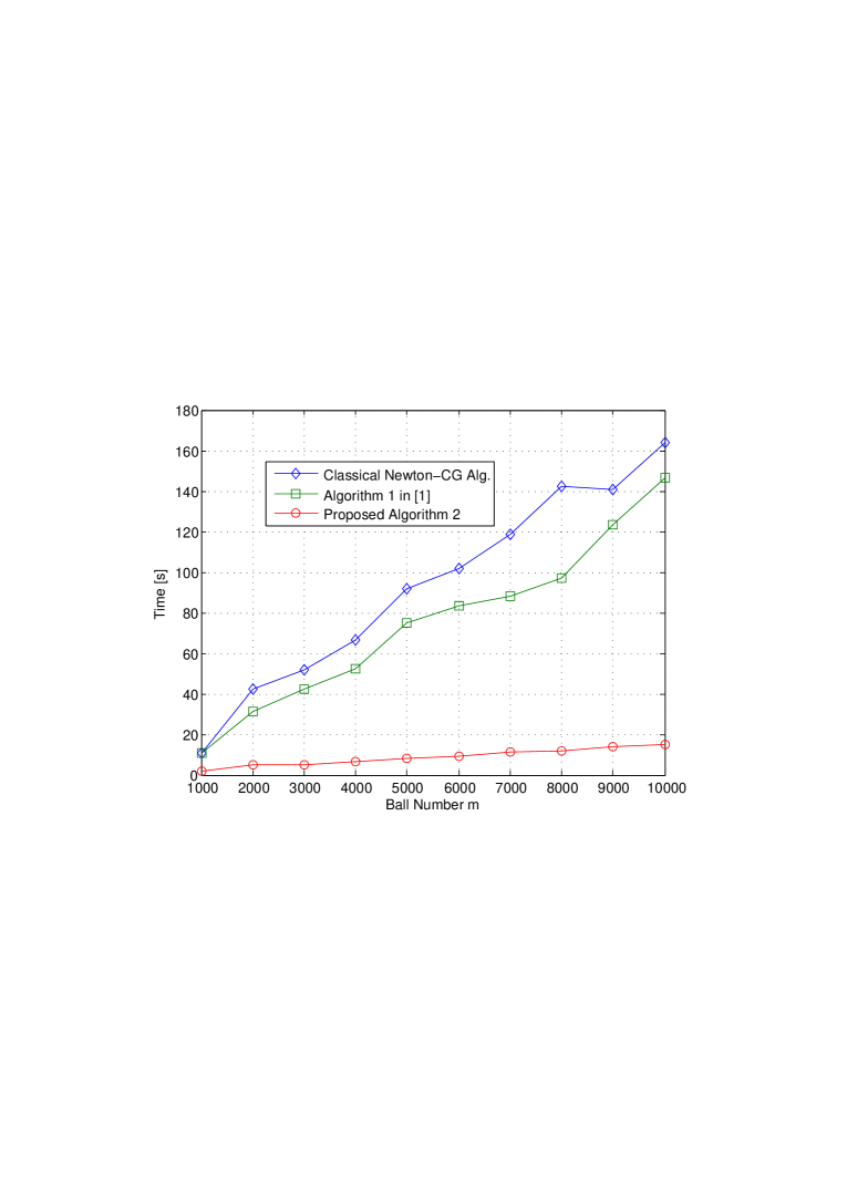
Figure 1: Time comparison of proposed Algorithm 2, Algorithm 1 in [1], and classical Newton-CG algorithm with different large $m$ and fixed $n=2000.$

We also plot the CPU time comparison of proposed Algorithm 2, Algorithm 1 in [1], and classical Newton-CG algorithm with different large $m$ and fixed $n=2000$ as Fig. 1. It can be observed from Fig. 1 that for fixed $n=2000$, the CPU time of all of three algorithms grow (approximately) linearly with $m.$ However, the CPU time of both Algorithm 1 and the classical Newton-CG algorithm grows much faster than that of proposed Algorithm 2.

In a nutshell, our numerical simulation results show that the proposed inexact Newton-CG algorithm is particularly amenable to solve the SEB problem of large dimensions. First, the gradient and Hessian-vector product are inexactly computed at each iteration of the proposed algorithm by exploiting the (approximate) sparsity structure of the log-exponential aggregation function. This dramatically reduces the computational cost compared to compute the gradient and Hessian-vector product exactly and thus makes the proposed algorithm well suited to solve the SEB problem with large $m.$ Second, at each iteration, the proposed algorithm computes the search direction by applying the CG method to solve the inexact Newton equation in an inexact fashion. This makes the proposed algorithm also very attractive to solving the SEB problem with large $n.$

6 Conclusions

In this paper, we developed a computationally efficient inexact Newton-CG algorithm for the SEB problem of large dimensions, which finds wide applications in pattern recognition, machine learning, support vector machines and so on. The key difference between the proposed inexact Newton-CG algorithm and the classical Newton-CG algorithm is that the gradient and the Hessian-vector product are inexactly computed in the proposed algorithm by exploiting the special (approximate) sparsity structure of its log-exponential aggregation function. We proposed an adaptive criterion of inexactly computing the gradient/Hessian and also established global convergence of the proposed algorithm. Simulation results show that the proposed algorithm significantly outperforms the classical Newton-CG algorithm and the state-of-the-art algorithm in [1] in terms of the computational CPU time. Although we focused on the SEB problem in this paper, the proposed algorithm can be applied to solve other min-max problems in [44, 45, 46, 47, 48, 49].

7 Acknowledgments

The authors wish to thank Professor Ya-xiang Yuan and Professor Yu-Hong Dai of State Key Laboratory of Scientific and Engineering Computing, Academy of Mathematics and Systems Science, Chinese Academy of Sciences, for their helpful comments on the paper. The authors also thank Professor Guanglu Zhou of Department of Mathematics and Statistics, Curtin University, for sharing the code of Algorithm 1 in [1].

References

• [1] Zhou G., Toh K.C., Sun J.: Efficient algorithms for the smallest enclosing ball problem. Comput. Optim. & Appl. 30, 147–160 (2005)
• [2] ReVelle C.S., Eiselt H.A.: Location analysis: A synthesis and survey. European J. Oper. Res. 165, 1–19 (2005)
• [3] Burges C.J.C.: A tutorial on support vector machines for pattern recognition. Data Min. Knowl. Disc. 2, 121–167 (1998)
• [4] Nielsen F., Nock R.: Approximating smallest enclosing balls with applications to machine learning. Int. J. Comput. Geom. & Appl. 19, 389–414 (2009)
• [5] Chung F.L., Deng Z., Wang S.: From minimum enclosing ball to fast fuzzy inference system training on large datasets. IEEE Trans. Fuzzy Sys. 17, 173–184 (2009)
• [6] Chapelle O., Vapnik V., Bousquet O., Mukherjee S.: Choosing multiple parameters for support vector machines. Mach. Learn. 46, 131–159 (2002)
• [7] Ben-Hur A., Horn D., Siegelmann H.T., Vapnik, V.: Support vector clustering. J. Mach. Learn. Res. 2, 125–137 (2001)
• [8] Cervantes J., Li X., Yu W., Li K.: Support vector machine classification for large data sets via minimum enclosing ball clustering. Neurocomput. 71, 611–619 (2008)
• [9] Bădoiu M., Har-Peled S., Indyk P.: Approximate clustering via core-sets. Proceedings of the 34th Annual ACM Symposium on Theory of Computing, 250–257 (2002)
• [10] Alon N., Dar S., Parnas M., Ron D.: Testing of clustering. SIAM Review 46, 285–308 (2004)
• [11] Deng Z., Chung F.L., Wang S.: FRSDE: Fast reduced set density estimator using minimal enclosing ball approximation. Pattern Recognition 41, 1363–1372 (2008)
• [12] Elzinga D.J., Hearn D.W.: The minimum covering sphere problem. Manage. Sci. 19, 96–104 (1972)
• [13] Hearn D.W., Vijan J.: Efficient algorithms for the (weighted) minimum circle problem. Oper. Res. 30, 777–795 (1982)
• [14] Xu S., Freund R.M., Sun J.: Solution methodologies for the smallest enclosing circle problem. Comput. Optim. & Appl. 25, 283–292 (2003)
• [15] Megiddo N.: Linear-time algorithms for linear programming in $\mathbb{R}^{3}$ and related problems. SIAM J. Comput. 12, 759–776 (1983)
• [16] Preparata F.P., Shamos M.I.: Computational Geometry: An Introduction, Texts and Monographs in Computer Science. Springer-Verlag, New York (1985)
• [17] Shamos M.I., Hoey D.: Closest-point problems. Proceeding of the 16th Annual Symposium on Foundations of Computer Science, 151–162 (1975)
• [18] Dyer M.: A class of convex programs with applications to computational geometry. Proceedings of the 8th Annual Symposium on Computational Geometry, 9–15 (1992)
• [19] Welzl E.: Smallest enclosing disks (balls and ellipsoids). Lecture Notes in Computer Science 555, 359–370 (1991)
• [20] Gärtner B., Schönherr S.: An efficient, exact, and generic quadratic programming solver for geometric optimization. Proceedings of the 16th Annual Symposium on Computational Geometry, 110–118 (2000)
• [21] Fischer K., Gärtner B.: The smallest enclosing ball of balls: combinatorial structure and algorithms. Int. J. Comput. Geometry & Appl. 14, 341–378 (2004)
• [22] Cheng D., Hu X., Martin C.: On the smallest enclosing balls. Commun. Inf. & Sys. 6, 137–160 (2006)
• [23] Boyd S., Mutapcic A.: Subgradient methods. Notes for EE364b, Standford University (Winter 2006–07)
• [24] Shor N.Z.: Minimization Methods for Non-Differentiable Functions. Springer-Verlag, New York (1985)
• [25] TüTüncü R.H., Toh K.C., Todd M.J.: Solving semidefinite-quadratic-linear programs using SDPT3. Math. Prog. Ser. B. 95, 189–217 (2003)
• [26] Xu S.: Smoothing method for minimax problems. Comput. Optim. & Appl. 20, 267–279 (2001)
• [27] Pan S.H., Li X.S.: An efficient algorithm for the smallest enclosing ball problem in high dimensions. Appl. Math. & Comput. 172, 49–61 (2006)
• [28] Nesterov Y.: Smooth minimization of non-smooth functions. Math. Prog., Ser. A. 103, 127–152 (2005)
• [29] Xiao Y., Yu B.: A truncated aggeregate smoothing Newton method for minimax problems. Appl. Math. & Comput. 216, 1868–1879 (2010)
• [30] Polak E., Royset J.O., Womersley R.S.: Algorithms with adaptive smoothing for finite minimax problems. J. Optim. Theory & Appl. 119, 459–484 (2003)
• [31] Polak E.: Optimization: Algorithms and Consistent Approximations. Springer-Verlag, New York (1997)
• [32] Zang I.: A smoothing-out technique for min-max optimization. Math. Prog. 19, 61–77 (1980)
• [33] Li J., Wu Z., Long Q.: A new objective penalty function approach for solving constrained minimax problems. J. Oper. Res. Soc. China 2, 93–108 (2014)
• [34] Lü Y.B., Wan Z.P.: A smoothing method for solving bilevel multiobjective programming problems. J. Oper. Res. Soc. China 2, 511–525 (2014)
• [35] Li X.S.: An aggregate function method for nonlinear programming. Sci. China Ser. A. 34, 1467–1473 (1991)
• [36] Li X.S., Fang S.C.: On the entropic regularization method for solving min-max problems with applications. Math. Methods Oper. Res. 46, 119–130 (1997)
• [37] Liu D.C., Nocedal J.: On the limited memory BFGS method for large scale optimization. Math. Prog. 45, 503–528 (1989)
• [38] Chen B., Harker P.T.: A non-interior-point continuation method for linear complementarity problems. SIAM J. Matrix Anal. & Appl. 14, 1168–1190 (1993)
• [39] Kanzow C.: Some noninterior continuation methods for linear complementarity problems. SIAM J. Matrix Anal. & Appl. 17, 851–868 (1996)
• [40] Smale S.: Algorithms for solving equations. Proceedings of International Congress of Mathematicians (1987)
• [41] Nocedal J., Wright S.J.: Numerical Optimization. Springer-Verlag, New York (1999)
• [42] Sun W., Yuan Y.X.: Optimization Theory and Methods: Nonlinear Programming. Springer Science+Business Media (2006)
• [43] Larsson T., Kälberg L.: Fast and robust approximation of smallest enclosing balls in arbitrary dimensions. Eurographics Symposium on Geometry Processing 32, 93–101 (2013)
• [44] Arkin E.M., Hassin R., Levin A.: Approximations for minimum and min-max vehicle routing problems. J. Algorithm 59, 1–18 (2006)
• [45] Cherkaev E., Cherkaev A.: Minimax optimization problem of structural design. Comput. & Struct. 86, 1426–1435 (2008)
• [46] Al-Subaihi I., Watson G.A.: Fitting parametric curves and surfaces by $l_{\infty}$ discrete regression. BIT Numer. Math. 45, 443–461 (2005)
• [47] Liu Y.F., Dai Y.H., Luo Z.Q.: Coordinated beamforming for MISO interference channel: Complexity analysis and efficient algorithms. IEEE Trans. Signal Process. 59, 1142–1157 (2011)
• [48] Liu Y.F., Hong M., Dai Y.H.: Max-min fairness linear transceiver design problem for a multi-user SIMO interference channel is polynomial time solvable. IEEE Signal Process. Lett. 20, 27–30 (2013)
• [49] Liu Y.F., Dai Y.H., Luo Z.Q.: Max-min fairness linear transceiver design for a multi-user MIMO interference channel. IEEE Trans. Signal Process. 61, 2413–1423 (2013)