An effective decomposition approach and heuristics to generate spanning trees with a small number of branch vertices

Abstract

Given a graph $G=(V,E)$, the minimum branch vertices problem consists in finding a spanning tree $T=(V,E^{\prime})$ of $G$ minimizing the number of vertices with degree greater than two. We consider a simple combinatorial lower bound for the problem, from which we propose a decomposition approach. The motivation is to break down the problem into several smaller subproblems which are more tractable computationally, and then recombine the obtained solutions to generate a solution to the original problem. We also propose effective constructive heuristics to the problem which take into consideration the problem’s structure in order to obtain good feasible solutions. Computational results show that our decomposition approach is very fast and can drastically reduce the size of the subproblems to be solved. This allows a branch and cut algorithm to perform much better than when used over the full original problem. The results also show that the proposed constructive heuristics are highly efficient and generate very good quality solutions, outperforming other heuristics available in the literature in several situations.

Keywords: minimum branch vertices, spanning tree, graph decomposition, heuristics, branch and cut, combinatorial optimization.

1 Introduction

Spanning tree problems with constraints and/or objective functions concerning the degrees of the vertices in the tree arise very often in the context of communication networks. In this paper we deal with the problem of finding spanning trees which minimize the number of branch vertices (vertices with degree greater than two), known in the literature as the minimum branch vertices problem (MBV).

The MBV was introduced in Gargano et al. [6, 7], motivated by the context of optical networks using a technology which allows a specific type of switch to replicate a signal by splitting light. Such a switch is required if a connection arrives at a given vertex of the network and has to be multicasted to different vertices. Therefore, a branch vertex in a network tree would imply the use of such a sophisticated switch. However, the availability of these switches is usually limited due to their costs, and one is asked to minimize their need in a network topology.

Several authors studied different theoretical properties concerning the number of branch vertices in a graph. Gargano et al. [6, 7] showed the problem to be NP-Hard, besides some additional complexity results. They also considered bounds on the number of branch vertices and certain algorithmic and combinatorial aspects regarding the existence of structures such as spanning spiders (trees with at most one branch vertex). Matsuda et al. [10] give bounds on the number of branch vertices in claw-free graphs.

Chimani and Spoerhase [5] developed a 6/11-approximation algorithm for the complement of the MBV, namely the maximum path-node spanning tree problem, which aims at finding a spanning tree maximizing the number of vertices with degree at most two.

Different integer programming and heuristic approaches were proposed to the MBV. Carrabs et al. [2] studied integer programming formulations and a Lagrangian relaxation approach able to generate good feasible solutions. Cerrone et al. [3] showed the relation between three problems: the minimum branch vertices, the minimum degree sum problem and the minimum leaves problem. They also presented an evolutionary algorithm which could be applied to these problems. Cerulli et al. [4] proposed three heuristics to the problem, exploiting vertex weighting, vertex coloring, and an approach combining the previous two. Silva et al. [14] proposed an iterative refinement local search procedure. Almeida et al. [1] used a constructive heuristic based on breadth-first search, together with some changes in the procedure described in [14]. Öncan [12] proposed inequalities to improve the linear relaxation bounds obtained with a polynomial size integer programming formulation to the problem. Rossi et al. [13] implemented a hybrid approach, combining a branch and cut algorithm with a tabu search heuristic, which could be applied to the MBV and to the minimum degree sum problem. Computational experiments showed that their approach outperformed the other integer programming techniques available in the literature. Very recently, Marín [9] proposed a preprocessing technique, valid inequalities and a heuristic algorithm, which combined could solve to optimality several instances used in the literature.

Our work aims at the development of an effective approach to solve the MBV. The remainder of the paper is organized as follows. Section 2 gives a formal statement of the problem together with an integer programming formulation containing an exponential number of inequalities. In Section 3 we give a simple algorithm to derive a combinatorial lower bound, which also determines important information that will be used in our graph decomposition approach. In Section 4 we present the decomposition method, which aims at dividing the problem into several smaller subproblems that are hopefully more manageable computationally. Two constructive heuristics, which try to take advantage of the problem’s structure and of what is expected of a good solution, are described in Section 5. In Section 6, we present computational results considering the proposed approaches together with a branch and cut algorithm using the formulation described in Section 2. Some final remarks are discussed in Section 7.

2 Problem definition and formulation

Let $G=(V,E)$ be a simple, connected, undirected graph with a set $V$ of vertices and a set $E$ of edges. Denote $d_{G}(v)$ the degree of $v\in V$ in $G$. A vertex $v\in V$ is a branch vertex if it has degree greater than two, i.e. $d_{G}(v)>2$. Given the graph $G$, the minimum branch vertices problem (MBV) consists in finding a spanning tree $T=(V,E^{\prime})$, with $E^{\prime}\subseteq E$, minimizing the number of branch vertices.

We now present an integer programming formulation for the problem containing an exponential number of constraints. Consider the variables:

$$x_{uv}=\left\{\begin{array}[]{l}1,\textrm{ if edge $(u,v)\in E$ is part of the tree,}\\ 0,\textrm{ otherwise;}\end{array}\right.$$

$$y_{v}=\left\{\begin{array}[]{l}1,\textrm{ if vertex $v\in V$ is a branch vertex,}\\ 0,\textrm{ otherwise.}\end{array}\right.$$

Using the variables just described, the MBV can be formulated as:

$$z=\min \quad\sum_{v\in V}y_{v}$$ (1)

s.t.

$$\sum_{(u,v)\in E}x_{uv}=|V|-1,\quad$$ (2)

$$\sum_{(u,v)\in E:u,v\in S}x_{uv}\leq|S|-1\ \ \ \quad {\rm for\ }S\subset V,$$ (3)

$$\sum_{u:(u,v)\in E}x_{uv}\leq 2+(d_{G}(v)-2)y_{v}\ \ \ \quad {\rm for\ }v\in V,$$ (4)

$$x\in\{0,1\}^{|E|},\quad\ y\in\{0,1\}^{|V|}.$$ (5)

The objective function (1) minimizes the number of branch vertices. Constraints (2) specify that exactly $|V|-1$ edges are selected. Constraints (3) are subtour elimination constraints; note that we only need to consider subsets $S$ such that $|S|>2$. Constraints (4) set the branch vertex variable associated to vertex $v$ to one in case more than two edges are incident to $v$. Constraints (5) are integrality requirements on the variables. It is worth mentioning that we can fix the $y_{v}$ variable at zero for any vertex $v\in V$ with degree lower or equal to two.

3 A combinatorial lower bound

In this section, we present an algorithm to calculate a combinatorial lower bound to the MBV problem, which also determines some important data to be used in a graph decomposition approach. Let $s(G)$ be the minimum number of branch vertices in any spanning tree of $G$. An articulation point (or cut vertex) is a vertex whose removal from the graph increases the number of components in the graph. A straightforward lower bound $\underline{s}(G)$ on the value of $s(G)$ can be calculated based on a simple observation of Gargano et al. [7]: any articulation point whose removal induces at least three connected components is necessarily a branch vertex in any spanning tree of $G$. We denote such vertices obligatory branches and define $L_{o}$ to be the set of obligatory branches of $G$.

Let $G-v$ be the subgraph of $G$ obtained by removing the vertex $v$ together with all its incident edges. We denote by $\alpha(v)$ the number of connected components of $G-v$. Note that $\alpha(v)\geq 2$ for an articulation point $v$, while $\alpha(v)\geq 3$ for any obligatory branch. Algorithm 1 calculates the lower bound $\underline{s}(G)$ on the number of branch vertices, the set of obligatory branches $L_{o}$ and the value of $\alpha(v)$ for every obligatory branch $v\in L_{o}$.

Algorithm 1 Obligatory branches lower bound

1:  $L_{o}\leftarrow\emptyset$

2:  $V^{\prime}\leftarrow$ list of articulation points in $G$

3:  for all $v\in V^{\prime}$ do

4:     $c\leftarrow$ number of connected components of $G-v$

5:     if $c\geq 3$ then

6:        $L_{o}\leftarrow L_{o}+\{v\}$

7:        $\alpha(v)\leftarrow c$

8:     end if

9:  end for

10:  $\underline{s}(G)\leftarrow|L_{o}|$

Observation 1.

Algorithm 1 runs in $O(|V|+|E|)$.

Proof.

The list of articulation points $V^{\prime}$ can be obtained in step 2 using a depth-first search (DFS) algorithm augmented with the opening time of each vertex, i.e. its visiting index in the DFS tree. In particular, we identify an articulation at a given vertex $u$ if, when the search at a neighbor $v$ returns, the oldest index (opened the earliest) reachable from $v$ is no smaller than the opening time of $u$. Finding $i$ articulations at a vertex means that the search started from it $i$ times, and that $i+1$ components are left after removing it, which is precisely the information used later in step 4.

The DFS algorithm runs in $O(|V|+|E|)$ when an adjacency list is used. The for loop (lines 3-9) is executed $|V^{\prime}|$ times, and all operations within it are performed in constant order of complexity. Therefore the algorithm runs in $O(|V|+|E|)+O(|V^{\prime}|)$ $=$ $O(|V|+|E|)$. ∎

Given that the MBV problem is NP-Hard, one should note that the lower bound obtained using Algorithm 1 is not necessarily tight. It is actually possible to find situations in which this occurs even for very small graphs. For instance, consider the graph illustrated in Figure 1, which does not have any obligatory branch vertex. Nevertheless, it is not difficult to check that either $b$ or $d$ should be a branch vertex in a spanning tree of the considered graph.

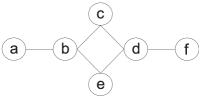
Figure 1: Example in which $\underline{s}(G)=0<s(G)=1$

4 Graph decomposition approach

In this section, we present a graph decomposition approach to the minimum branch vertices problem based on two different properties of a graph. The first one is grounded on the existence of obligatory branch vertices. The second builds on the existence of cut edges (or bridges): an edge whose removal increases the number of connected components of a graph. This decomposition approach aims at dividing the original MBV problem into smaller subproblems, that can be solved separately and then recombined in order to generate a solution to the original problem. We remark that Marín [9] proposed a preprocessing routine, which included the identification of cut edges, but that information was not used in a decomposition method by the author.

4.1 Obligatory branches based decomposition

This first decomposition is based on the fact that an obligatory branch $v\in V(G)$ is going to be a branch vertex in any spanning tree of a graph $G$. Starting from $G=(V,E)$, we build a new graph $G_{o}=(V_{o},E_{o})$ as follows. Initially, $V_{o}=V$ and $E_{o}=E$, such that $G_{o}=(V,E)$. Next, for each obligatory branch $v\in L_{o}$, create $\alpha(v)$ new vertices $\{v_{1},\ldots,v_{\alpha(v)}\}$ and add them to $V_{o}$. Let $N_{i}(v)$ be the set of vertices to which $v$ is adjacent in the $i-th$ connected component of the subgraph $G-v$. For each $i\in\{1,\ldots,\alpha(v)\}$, create in $E_{o}$ edges from $v_{i}$ to every vertex in $N_{i}(v)$. After that, remove $v$ from $V_{o}$ and all its adjacent edges from $E_{o}$.

The obligatory branches based decomposition is illustrated in Figure 2 for a graph with two obligatory branches.

(a) Original graph with obligatory branches $c$ and $g$

(b) Applying decomposition for obligatory branches $c$ and $g$

Figure 2: Illustration of the obligatory branches based decomposition

4.2 Cut edges based decomposition

This decomposition is based on the fact that every cut edge must be in any spanning tree of $G$. Starting from a graph $G=(V,E)$, let $B=\{(u,v)\in E:(u,v)\textrm{ is a cut edge in G}\}$.

A new graph $G^{\prime}$ can be obtained from $G$ by removing from $E$ every edge $(u,v)\in B$. For the sake of correctness of the formulation for each resulting subproblem defined over $G^{\prime}$ (see Section 4.3), we need the information of extra degree corresponding to both end vertices of the cut edges removed in $G^{\prime}$. Let $\gamma(v)$ be the extra degree of a vertex $v$, which corresponds to the number of cut edges $(u,v)\in B$ incident to $v$ in the initial graph $G$.

The cut edges based decomposition is illustrated in Figure 3 for a graph with two cut edges.

(a) Original graph with cut edges $(a,f)$ and $(c,d)$

(b) Applying decomposition for cut edges $(a,f)$ and $(c,d)$, which implies $\gamma(a)=\gamma(f)=\gamma(c)=\gamma(d)=1$

Figure 3: Illustration of the cut edges based decomposition

4.3 The decomposed problem

We now give an integer programming formulation aimed at solving each component of the decomposed problem as an independent subproblem. Let $G^{\prime}_{o}=(V^{\prime}_{o},E^{\prime}_{o})$ be the resulting graph after performing the obligatory branches and cut edges based decompositions. Observe that $G^{\prime}_{o}$ is disconnected in case at least one obligatory branch or one cut edge was found.

Let $K$ be the number of connected components in $G^{\prime}_{o}$, and ${G^{\prime}}_{o}^{k}=({V^{\prime}}_{o}^{k},{E^{\prime}}_{o}^{k})$ be the $k-th$ connected subgraph of $G^{\prime}_{o}$, with $k\in\{1,\ldots,K\}$. Define the set ${\overline{V}^{\prime}}^{k}_{o}=\{v\in{V^{\prime}}^{k}_{o}:v\textrm{ was not artificially created based on }L_{o}\}$. A formulation for each of the $k$ connected components can be obtained as:

$$z_{k}=\min \quad\sum_{v\in\overline{V}^{\prime k}_{o}}y_{v}$$ (6)

s.t.

$$\sum_{(u,v)\in{E^{\prime}}_{o}^{k}}x_{uv}=|{V^{\prime}}^{k}_{o}|-1,\quad$$ (7)

$$\sum_{(u,v)\in{E^{\prime}}_{o}^{k}:u,v\in S}x_{uv}\leq|S|-1\ \ \ \quad {\rm for\ }S\subset{V^{\prime}}^{k}_{o},$$ (8)

$$\sum_{u:(u,v)\in{E^{\prime}}_{o}^{k}}x_{uv}+\gamma(v)\leq 2+(d_{G}(v)-2)y_{v}\ \ \ \quad {\rm for\ }v\in{\overline{V}^{\prime}}^{k}_{o},$$ (9)

$$x\in\{0,1\}^{|{E^{\prime}}_{o}^{k}|},\quad\ y\in\{0,1\}^{|{V^{\prime}}^{k}_{o}|}.$$ (10)

Proposition 1.

An optimal solution to the minimum branch vertices problem can be obtained from the solutions of the $K$ connected components of $G^{\prime}_{o}$ and its optimal value is

$$z=|L_{o}|+\sum_{k=1}^{K}z_{k}.$$

Proof.

By definition, each obligatory branch should contribute with one unit to the objective function $z$. Since they are not considered in the decomposed objective functions $z_{k}$, the $|L_{o}|$ units have to be added to $z$.

Since every cut edge $(u,v)\in B$ must be in the spanning tree, the values $\gamma(u)$ and $\gamma(v)$ of its incident vertices will guarantee that the additional degree corresponding to these edges will be taken into account in ${G^{\prime}}^{k}_{o}$. Considering an obligatory branch $v$, there are no edges linking vertices between two different components in the original graph without $v$, i.e. $G-v$. Therefore the different components of $G-v$ directly implied by the removal of $v$ have to be connected through the edges incident to $v$ in $G$.

In every connected component ${G^{\prime}}^{k}_{o}$, we obtain a spanning tree minimizing the number of branch vertices, disregarding the obligatory branches implied by $L_{o}$. The different trees will be connected to the other components in the original graph via either the obligatory branch vertices or the cut edges. The resulting forest implies thus a spanning tree with minimum number of branch vertices in the original graph $G$. ∎

5 Heuristic algorithms

We noted that the heuristics available in the literature for the MBV do not take advantage of the problem’s structure in order to generate good feasible solutions. Instead, they concentrate into the improvement of available solutions. We present two simple constructive heuristic algorithms to the MBV that take the structure of the problem into consideration in an attempt to obtain high quality solutions.

The key observation is the fact that in an ideal situation (one in which no branch vertices are necessary), the optimal spanning tree to the problem should be a branch vertex free solution, i.e. a Hamiltonian path. Observe also that good solutions will tend to have paths that are as long as possible connected to each other via some branch vertices. The two constructive heuristics presented in this section take this into consideration.

5.1 Path expanding heuristic

The basic idea of the path expanding heuristic is to, starting from a tree $T$ with a single vertex, constructively turn $T$ into a spanning tree by expanding paths already in $T$. The algorithm has two main components, namely a start-restart in which a new vertex is selected as source of a new path and a path expansion in which new vertices are added to the path being expanded. The greedy criteria for the two components are:

• start-restart (enumerated in order of priority):

  1. obligatory branch vertex;

  2. vertex whose degree is already greater than two in the tree;

  3. vertex with the largest number of neighbors which are still not in the tree;

• path expansion: vertex, adjacent to the latest one added to the tree, with the smallest number of neighbors which are still not in the tree.

The heuristic is presented in Algorithm 2 and it works as follows. Start the tree with a vertex selected according to the start-restart greedy criterion. Build a path starting at a vertex already belonging to the partial tree, selecting the next vertices in this path according to the path expansion criterion until it can no longer be expanded. If there are still vertices not belonging to the tree, another vertex with unvisited neighbors in the partial tree is selected and a new path is constructed starting from the current tree. The algorithm is illustrated in Figure 4.

Algorithm 2 Path-Expanding($G=(V,E)$)

1:  $V(T)\leftarrow\{u\}$, with $u$ selected according to the start-restart criterion

2:  while $|T|<|V|-1$ do

3:     select a vertex $u\in V(T)$ with neighbors still not in $V(T)$ and degree at most 1, if any exists; otherwise, select the best vertex according to the start-restart criterion

4:     while $u$ has neighbors not belonging to $V(T)$ do

5:        $v\leftarrow$ best neighbor of $u$ according to the path expansion criterion such that $v\notin V(T)$

6:        $V(T)\leftarrow V(T)+\{v\}$

7:        $T\leftarrow T+\{(u,v)\}$

8:        $u\leftarrow v$

9:     end while

10:  end while

11:  return  $T$

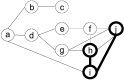
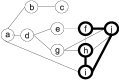
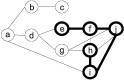
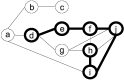
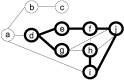
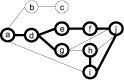
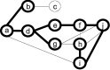
Figure 4: Illustration of the path expanding heuristic. The vertices and edges in bold are those belonging to the tree being constructed.

Observation 2.

Algorithm 2 runs in $O(|V|^{2})$.

Proof.

A single evaluation of the start-restart or the path expansion criteria can be done in time proportional to $O(|V|)$, as it requires checking information available at each vertex. In particular, note that checking the number of neighboring vertices which are still not in the tree, e.g. the last start-restart criterion and the inner loop condition, can be kept at constant asymptotic complexity, provided that we update this information when the tree is grown.

The number of iterations of the outer and the inner while loops depends on the particular graph, but they sum to $|V|-1$ since these correspond to the selection of edges in a spanning tree. Therefore, the execution includes $|V|-1$ steps, each requiring an $O(|V|)$ evaluation (either start-restart or path expansion) and $O(|V|)$ operations to update the aforementioned information on the remaining vertices. The algorithm thus runs in time proportional to $O(|V|-1)\times(O(|V|)+O(|V|))=O(|V|^{2})$. ∎

5.2 Multi-path expanding heuristic

The multi-path expanding heuristic differs from the path expanding heuristic in the fact that it allows the expansion of any of the paths being expanded at a given moment. It also has a start-restart component, which is the same for the path-expanding heuristic. The multi-path expansion component uses the following greedy criterion:

• multi-path expansion: vertex, adjacent to any vertex belonging to the tree, with the smallest number of neighbors which are still not in the tree.

The multi-path expanding heuristic is presented in Algorithm 3 and it works in the following way. Start the tree with a given vertex, selected according to the start-restart greedy criterion, which forms the list of candidates for path expansion. Continue selecting a vertex adjacent to one of the candidates for path expansion according to the multi-path expansion greedy criterion, add the new vertex to the list of candidates and remove the current candidate from the list of candidates when appropriate. If there are no more vertices, which are still not in the tree, adjacent to the candidates and if the tree is still not a spanning tree, select another vertex to add to the list of candidates. The algorithm is illustrated in Figure 5.

Algorithm 3 Multi-Path-Expanding($G=(V,E)$)

1:  $V(T)\leftarrow\{u\}$, with $u$ selected according to the start-restart criterion

2:  $Cand\leftarrow\varnothing$

3:  while $|T|<|V|-1$ do

4:     $Cand\leftarrow Cand\cup\{u\},u\in V(T)$ according to the start-restart criterion

5:     while  $\exists(u,v)$ such that $u\in Cand$ and $v\notin V(T)$ do

6:        select such $(u,v)$ optimizing the multi-path expansion criterion

7:        $T\leftarrow T+\{(u,v)\}$

8:        $V(T)\leftarrow V(T)+\{v\}$

9:        if $d_{T}(u)=2$ and $u\notin L_{0}$ then

10:           $Cand\leftarrow Cand-\{u\}$

11:        end if

12:        $Cand\leftarrow Cand+\{v\}$

13:     end while

14:  end while

15:  return  $T$

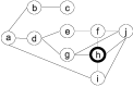
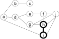
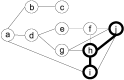
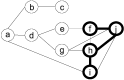
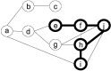
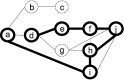
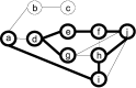
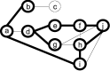
Figure 5: Illustration of the multi-path expanding heuristic. The vertices and edges in bold are those belonging to the tree being constructed.

Observation 3.

Algorithm 3 runs in $O(|V|^{2})$.

Proof.

The analysis is analogous to that for Algorithm 2. The main difference is that, to keep the multi-path expansion test in $O(|V|)$ time, we need to store the additional information of whether a given unvisited vertex is adjacent to one in the tree. This can be included in the structure update without increasing its asymptotic complexity. The operations introduced due to the candidates set are done in constant order of complexity.

Again, there is a total of $|V|-1$ iterations considering both while loops, each selecting a new edge in the tree. When needed, choosing a vertex to enter the set of candidates is done following the same start-restart criterion, in time $O(|V|)$. In the inner loop, both the multi-path expansion and the updating step require $O(|V|)$ time. Therefore, the algorithm requires computational time proportional to $O(|V|-1)\times(O(|V|)+O(|V|))=O(|V|^{2})$. ∎

6 Computational experiments

The main goal of our computational experiments is to assess the effectiveness of the methods proposed in this paper. The branch and cut algorithm presented by Rossi et al. [13] is based on the formulation (1)–(5), and it is a state-of-the-art among exact approaches to solve the MBV . We implemented our own branch and cut algorithm using the formulation (1)–(5), and refer to it as the plain algorithm. Our main results compare it against one variant developed on top of the decomposition and primal heuristics we proposed in previous sections: henceforth, the enhanced algorithm, using formulation (6)–(10).

The algorithms are implemented in C++, using the callback mechanism in the Concert API of CPLEX 12.6. Since the objective function is integer-valued for all the available instances, we set the parameter regarding the absolute MIP gap tolerance to $0.9999$; all remaining options are used as default. Also, the best solution among the path-expanding and the multi-path-expanding heuristics is given as a MIP start to the solver. Experiments were carried out on a machine with an Intel Core i7-4790K (4.00GHz) CPU, with 16GB of RAM. A time limit of one hour (3600s wall clock) was imposed for every execution.

We remark that the whole procedure consisting of the decomposition and the constructive methods runs immediately for all the available benchmark instances. Considering any of those instances, the decomposed integer programming (IP) models and heuristic solutions were created in less than $0.02$ seconds.

Most papers on the MBV use the large benchmark set of Carrabs et al. [2], which includes 525 instances. Section 6.1 reports results using that benchmark. Nevertheless, Silva et al. [14] introduced different sets of instances; for the sake of completeness, we discuss in Section 6.2 the effectiveness of the procedures using those problem sets as well.

6.1 Instances from Carrabs et al. [2]

We describe next our computational results using the standard benchmark of Carrabs et al. [2], which was also used in [12, 13]. The instances are identified as Spd_RF2_n_m_r, in which $n$ stands for the number of vertices, $m$ for the number of edges, and $r$ the seed used to randomly generate the edges of the graph.

We start by describing the effect of the decomposition and comparing the plain and enhanced algorithms. Table LABEL:tab:openInstances presents the results for all instances for which an optimal solution was not found by the plain algorithm within the one hour time limit. The second and third columns indicate the number of obligatory branches (OB) and cut edges (CE) removed using the decomposition algorithm. The next three columns concern the enhanced algorithm, and show the best lower and upper bounds and the remaining open gap (in %) between them at the end of the execution. The last three columns give the same information for the plain algorithm. We also show the time taken for the enhanced algorithm to solve the instances to optimality (the value 3600 is shown in case the instance remained unsolved at the end of the time limit). The arithmetic mean is used for average values.

In the comparison, we argue in favor of the enhanced algorithm for two main reasons. First, it is consistently superior in finding better solutions for the MBV. Note that the enhanced algorithm yields a smaller duality gap in 48 out of 50 instances ($96\%$). In fact, it is able to close the gap of 39 among these instances ($78\%$).

Table 1: Results regarding instances for which the plain branch and cut algorithm cannot prove optimality within one hour of computation. For the starred instances, the enhanced algorithm is worse than the plain version.

Instance	Reduction			Enhanced Algorithm					Plain Algorithm
	OB	CE		LB	UB	Gap (%)	Time (s)		LB	UB	Gap (%)
Spd_RF2_400_519_4731	52	155		70	70	0	227.9		67.66	70	3.3
Spd_RF2_450_548_4915	68	205		89	89	0	324.4		88.00	89	1.1
Spd_RF2_450_581_4947	59	178		76.38	80	4.5	3600.0		75.86	80	5.2
Spd_RF2_450_581_4963	61	178		77	77	0	125.8		75.81	78	2.8
Spd_RF2_450_614_4979*	45	149		64.35	67	4.0	3600.0		64.34	66	2.5
Spd_RF2_450_614_5003	44	153		67	67	0	901.8		64.55	68	5.1
Spd_RF2_500_603_5091	90	264		109	109	0	176.1		107.37	109	1.5
Spd_RF2_500_672_5171	58	180		79.72	82	2.8	3600.0		78.24	81	3.4
Spd_RF2_500_672_5179	52	171		75.45	77	2.0	3600.0		73.83	78	5.3
Spd_RF2_500_672_5187*	47	155		69.51	72	3.5	3600.0		69.53	71	2.1
Spd_RF2_500_672_5195	57	171		77	77	0	2128.6		75.69	78	3.0
Spd_RF2_500_672_5203	57	173		74.58	76	1.9	3600.0		73.47	78	5.8
Spd_RF2_600_749_5355	136	370		143	143	0	462.7		142.00	143	0.7
Spd_RF2_700_821_5523	164	467		182	182	0	12.6		180.71	183	1.3
Spd_RF2_700_861_5563	151	437		159.67	161	0.8	3600.0		159.72	161	0.8
Spd_RF2_700_902_5579	143	408		152	152	0	1106.3		150.73	153	1.5
Spd_RF2_700_902_5595	143	401		153	153	0	130.7		151.86	154	1.4
Spd_RF2_800_886_5659	212	601		227	227	0	10.5		225.67	228	1.0
Spd_RF2_800_930_5715	200	549		212	212	0	49.0		209.42	213	1.7
Spd_RF2_800_973_5747	183	506		197	197	0	3461.6		194.36	198	1.8
Spd_RF2_800_973_5763	179	504		195	195	0	1057.0		191.11	197	3.0
Spd_RF2_800_1017_5771	164	470		176	176	0	1208.5		173.50	178	2.5
Spd_RF2_800_1017_5779	158	467		173	173	0	2375.2		171.25	173	1.0
Spd_RF2_800_1017_5787	165	468		178	178	0	108.6		175.71	181	2.9
Spd_RF2_900_989_5859	238	688		259	259	0	63.7		254.08	259	1.9
Spd_RF2_900_1034_5891	228	640		242	242	0	23.9		238.78	243	1.7
Spd_RF2_900_1034_5907	220	621		239	239	0	1411.3		236.19	240	1.6
Spd_RF2_900_1034_5915	228	642		242	242	0	466.1		238.99	243	1.7
Spd_RF2_900_1079_5931	206	579		222	222	0	332.6		218.77	223	1.9
Spd_RF2_900_1079_5939	207	580		224	224	0	349.5		220.67	226	2.4
Spd_RF2_900_1079_5947	210	582		226	226	0	888.0		220.81	230	4.0
Spd_RF2_900_1079_5963	205	588		222	222	0	27.9		218.52	223	2.0
Spd_RF2_900_1124_5971	198	543		210	210	0	836.7		207.86	210	1.0
Spd_RF2_900_1124_5979	198	549		210	210	0	167.9		207.16	210	1.4
Spd_RF2_900_1124_5987	190	546		203	203	0	340.6		201.54	204	1.2
Spd_RF2_900_1124_6003	189	549		202	202	0	3120.8		199.06	203	1.9
Spd_RF2_1000_1143_6091	252	704		272	272	0	2334.6		268.02	274	2.2
Spd_RF2_1000_1143_6099	254	711		271	271	0	9.5		268.24	272	1.4
Spd_RF2_1000_1143_6107	251	698		272	272	0	108.1		267.17	273	2.1
Spd_RF2_1000_1143_6115	253	700		272	272	0	314.5		269.87	272	0.8
Spd_RF2_1000_1143_6123	251	712		269	269	0	906.0		268.40	270	0.6
Spd_RF2_1000_1191_6131	228	662		247.67	249	0.5	3600.0		243.83	250	2.5
Spd_RF2_1000_1191_6139	235	659		251	251	0	362.4		248.11	252	1.5
Spd_RF2_1000_1191_6147	233	656		250	250	0	945.6		246.47	251	1.8
Spd_RF2_1000_1191_6155	235	655		253	253	0	193.9		251.54	253	0.6
Spd_RF2_1000_1239_6171	218	608		232	232	0	90.9		230.11	232	0.8
Spd_RF2_1000_1239_6179	222	605		236	237	0.4	3600.0		231.26	239	3.2
Spd_RF2_1000_1239_6187	217	611		229.81	233	1.4	3600.0		225.33	237	4.9
Spd_RF2_1000_1239_6195	222	616		238.01	241	1.2	3600.0		229.71	243	5.5
Spd_RF2_1000_1239_6203	218	609		236	236	0	2850.6		230.84	237	2.6
Average	20.4%	48.1%				0.46					2.3

For all the 475 remaining cases in this benchmark, the enhanced algorithm makes finding optimal solutions for the MBV a much faster task, as we present in Table LABEL:tab:solvedInstances. Given the large number of instances, we present the arithmetic mean after aggregating the results for instances with the same number of vertices (n) and edges (m). Regarding the smaller instances set (up to 500 vertices), the decomposition approach is able to reduce 15.9% of the vertices and 38.6% of the edges, on average, thus yielding the optimal solution in a smaller amount of time. As for the larger instances set (from 600 to 1,000 vertices), the average reduction is of 24.8% of the vertices and 61.3% of the edges, achieving a solution much faster.

Table 2: Results regarding instances for which both the plain branch and cut algorithm and the enhanced one are able to prove optimality within one hour of computation. The enhanced algorithm features the decomposition and heuristic methods. Columns OB and CE indicate the number of obligatory branches and cut edges removed, respectively.

Instances		Reduction Avg.		Time Avg. (s)		Instances		Reduction Avg.		Time Avg. (s)
n	m	OB	CE	Enhanced	Plain	n	m	OB	CE	Enhanced	Plain
200	222	45.8	127.8	0.1	1.5	600	637	173.0	493.6	0.8	26.7
200	244	32.2	92.4	1.1	4.4	600	674	156.2	437.4	5.3	131.9
200	267	23.4	69.0	1.6	10.0	600	712	139.6	394.4	143.0	406.6
200	289	15.4	56.8	78.5	77.2	600	749	129.8	361.8	55.9	837.8
200	312	11.0	42.2	11.5	15.2	600	787	119.4	333.6	202.9	849.3
250	273	60.0	164.4	0.1	2.8	700	740	203.0	576.8	0.7	52.0
250	297	43.2	120.8	3.0	14.9	700	780	185.2	518.4	9.3	242.5
250	321	34.2	101.8	3.2	14.5	700	821	167.3	471.0	54.8	1285.6
250	345	24.4	76.2	42.9	76.5	700	861	154.8	436.5	758.4	241.9
250	369	16.8	60.0	63.6	59.2	700	902	147.0	402.3	25.0	773.5
300	326	73.2	203.0	0.3	5.3	800	1017	167.0	468.0	222.2	325.2
300	353	57.8	160.2	3.8	17.8	800	843	232.0	666.8	1.2	69.4
300	380	43.0	124.8	20.1	57.4	800	886	213.8	599.0	5.4	503.8
300	407	34.4	104.6	60.0	117.2	800	930	193.5	546.0	8.4	343.1
300	434	25.6	86.4	279.0	146.2	800	973	180.0	506.3	1183.7	2598.0
350	378	85.4	238.8	0.6	7.9	900	1034	222.5	631.0	54.4	616.9
350	406	67.4	190.0	12.3	48.2	900	1079	207.0	589.0	171.9	775.6
350	435	50.4	151.0	359.2	402.0	900	1124	197.0	551.0	76.0	870.5
350	463	40.2	124.2	514.6	1059.5	900	944	262.2	756.4	1.7	111.5
350	492	29.0	103.5	73.3	262.5	900	989	242.0	685.0	36.6	941.7
400	429	102.4	282.6	0.8	39.4	1000	1047	296.2	849.6	3.8	222.3
400	459	78.6	226.4	11.1	53.2	1000	1095	268.8	767.0	32.8	820.0
400	489	62.2	184.8	44.0	228.4	1000	1191	233.0	656.0	634.6	1524.8
400	519	51.0	154.0	322.6	1198.5
400	549	41.8	131.2	700.5	1058.8
450	482	115.0	318.6	0.9	44.5
450	515	91.6	250.6	17.4	308.5
450	548	74.0	209.8	44.3	442.5
450	581	62.0	177.5	452.8	594.3
450	614	47.7	152.3	909.5	1278.0
500	534	131.8	361.0	1.5	46.7
500	568	106.0	294.2	26.8	256.4
500	603	86.0	241.5	318.5	1404.5
500	637	71.8	210.6	556.6	2103.1
Average:		15.9%	38.6%	145.2	337.0	Average:		24.8%	61.3%	160.4	633.5

Finally, we compare the performance of our heuristics with the best primal feasible solution cost obtained by the Lagrangian heuristics of Carrabs et al. [2]. The authors compiled their best bounds on a set of 175 problem instances. Table LABEL:tab:heuristicsCarrabs compares those values with the ones provided by our heuristics; we report the best value among the path-expanding and the multi-path expanding algorithms.

We highlight that our proposed constructive algorithms provide better warm starts. In fact, they provide better primal bounds to 103 instances. On the other hand, the best result presented by Carrabs et al. [2] is better in 54 instances, and is equal to the solution obtained with our constructive algorithms in 18 instances.

Table 3: Best primal solution constructed by our proposed algorithms and by the Lagrangian heuristic of Carrabs et al. [2]. Values in bold indicate the 103 instances (out of 175) in which our heuristics provide a better solution.

Instance	Best constructed	Best result	Instance	Best constructed	Best result
	solution	by [2]		solution	by [2]
Spd_RF2_200_222_3811	55	54	Spd_RF2_350_435_4515	81	77
Spd_RF2_200_222_3819	55	54	Spd_RF2_350_435_4523	75	74
Spd_RF2_200_222_3827	53	51	Spd_RF2_350_463_4531	69	70
Spd_RF2_200_222_3835	54	52	Spd_RF2_350_463_4539	70	70
Spd_RF2_200_222_3843	55	54	Spd_RF2_350_463_4547	67	71
Spd_RF2_200_244_3851	43	46	Spd_RF2_350_463_4555	68	70
Spd_RF2_200_244_3859	46	49	Spd_RF2_350_463_4563	66	73
Spd_RF2_200_244_3867	45	43	Spd_RF2_350_492_4571	55	62
Spd_RF2_200_244_3875	42	43	Spd_RF2_350_492_4579	62	64
Spd_RF2_200_244_3883	45	45	Spd_RF2_350_492_4587	59	60
Spd_RF2_200_267_3891	36	37	Spd_RF2_350_492_4595	59	57
Spd_RF2_200_267_3899	37	39	Spd_RF2_350_492_4603	59	63
Spd_RF2_200_267_3907	37	37	Spd_RF2_400_429_4611	118	118
Spd_RF2_200_267_3915	36	39	Spd_RF2_400_429_4619	118	116
Spd_RF2_200_267_3923	36	41	Spd_RF2_400_429_4627	115	116
Spd_RF2_200_289_3931	28	30	Spd_RF2_400_429_4635	117	115
Spd_RF2_200_289_3939	29	35	Spd_RF2_400_429_4643	118	117
Spd_RF2_200_289_3947	31	35	Spd_RF2_400_459_4651	106	105
Spd_RF2_200_289_3955	31	34	Spd_RF2_400_459_4659	101	100
Spd_RF2_200_289_3963	30	32	Spd_RF2_400_459_4667	102	106
Spd_RF2_200_312_3971	24	23	Spd_RF2_400_459_4675	104	106
Spd_RF2_200_312_3979	23	27	Spd_RF2_400_459_4683	103	103
Spd_RF2_200_312_3987	26	29	Spd_RF2_400_489_4691	87	87
Spd_RF2_200_312_3995	23	26	Spd_RF2_400_489_4699	92	98
Spd_RF2_200_312_4003	28	30	Spd_RF2_400_489_4707	90	95
Spd_RF2_250_273_4011	71	71	Spd_RF2_400_489_4715	91	88
Spd_RF2_250_273_4019	70	66	Spd_RF2_400_489_4723	92	92
Spd_RF2_250_273_4027	70	69	Spd_RF2_400_519_4731	79	83
Spd_RF2_250_273_4035	71	69	Spd_RF2_400_519_4739	77	85
Spd_RF2_250_273_4043	67	70	Spd_RF2_400_519_4747	79	82
Spd_RF2_250_297_4051	60	60	Spd_RF2_400_519_4755	80	85
Spd_RF2_250_297_4059	61	63	Spd_RF2_400_519_4763	78	84
Spd_RF2_250_297_4067	57	56	Spd_RF2_400_549_4771	68	77
Spd_RF2_250_297_4075	59	63	Spd_RF2_400_549_4779	66	73
Spd_RF2_250_297_4083	61	60	Spd_RF2_400_549_4787	72	71
Spd_RF2_250_321_4091	52	57	Spd_RF2_400_549_4795	71	69
Spd_RF2_250_321_4099	50	53	Spd_RF2_400_549_4803	73	75
Spd_RF2_250_321_4107	49	51	Spd_RF2_450_482_4811	131	128
Spd_RF2_250_321_4115	48	54	Spd_RF2_450_482_4819	130	130
Spd_RF2_250_321_4123	50	54	Spd_RF2_450_482_4827	133	133
Spd_RF2_250_345_4131	39	41	Spd_RF2_450_482_4835	132	133
Spd_RF2_250_345_4139	48	47	Spd_RF2_450_482_4843	132	130
Spd_RF2_250_345_4147	45	44	Spd_RF2_450_515_4851	116	118
Spd_RF2_250_345_4155	44	45	Spd_RF2_450_515_4859	118	118
Spd_RF2_250_345_4163	41	47	Spd_RF2_450_515_4867	112	120
Spd_RF2_250_369_4171	38	38	Spd_RF2_450_515_4875	118	118
Spd_RF2_250_369_4179	33	35	Spd_RF2_450_515_4883	117	114
Spd_RF2_250_369_4187	35	37	Spd_RF2_450_548_4891	109	105
Spd_RF2_250_369_4195	35	38	Spd_RF2_450_548_4899	101	105
Spd_RF2_250_369_4203	36	40	Spd_RF2_450_548_4907	100	101
Spd_RF2_300_326_4211	86	85	Spd_RF2_450_548_4915	101	106
Spd_RF2_300_326_4219	87	83	Spd_RF2_450_548_4923	105	107
Spd_RF2_300_326_4227	87	85	Spd_RF2_450_581_4931	93	93
Spd_RF2_300_326_4235	85	85	Spd_RF2_450_581_4939	90	93
Spd_RF2_300_326_4243	85	84	Spd_RF2_450_581_4947	95	99
Spd_RF2_300_353_4251	75	73	Spd_RF2_450_581_4955	91	97
Spd_RF2_300_353_4259	73	72	Spd_RF2_450_581_4963	90	96
Spd_RF2_300_353_4267	77	77	Spd_RF2_450_614_4971	82	90
Spd_RF2_300_353_4275	77	76	Spd_RF2_450_614_4979	80	88
Spd_RF2_300_353_4283	75	76	Spd_RF2_450_614_4987	79	85
Spd_RF2_300_380_4291	65	69	Spd_RF2_450_614_4995	79	86
Spd_RF2_300_380_4299	66	66	Spd_RF2_450_614_5003	83	87
Spd_RF2_300_380_4307	62	64	Spd_RF2_500_534_5011	147	145
Spd_RF2_300_380_4315	58	63	Spd_RF2_500_534_5019	148	147
Spd_RF2_300_380_4323	62	66	Spd_RF2_500_534_5027	150	146
Spd_RF2_300_407_4331	56	60	Spd_RF2_500_534_5035	150	148
Spd_RF2_300_407_4339	60	58	Spd_RF2_500_534_5043	147	145
Spd_RF2_300_407_4347	53	63	Spd_RF2_500_568_5051	129	128
Spd_RF2_300_407_4355	53	56	Spd_RF2_500_568_5059	129	132
Spd_RF2_300_407_4363	56	59	Spd_RF2_500_568_5067	131	132
Spd_RF2_300_434_4371	46	50	Spd_RF2_500_568_5075	133	131
Spd_RF2_300_434_4379	45	47	Spd_RF2_500_568_5083	130	132
Spd_RF2_300_434_4387	46	47	Spd_RF2_500_603_5091	118	125
Spd_RF2_300_434_4395	48	53	Spd_RF2_500_603_5099	116	115
Spd_RF2_300_434_4403	49	56	Spd_RF2_500_603_5107	122	121
Spd_RF2_350_378_4411	100	99	Spd_RF2_500_603_5115	116	123
Spd_RF2_350_378_4419	99	96	Spd_RF2_500_603_5123	116	117
Spd_RF2_350_378_4427	102	100	Spd_RF2_500_637_5131	106	112
Spd_RF2_350_378_4435	99	97	Spd_RF2_500_637_5139	105	108
Spd_RF2_350_378_4443	100	98	Spd_RF2_500_637_5147	102	107
Spd_RF2_350_406_4451	89	91	Spd_RF2_500_637_5155	101	106
Spd_RF2_350_406_4459	89	87	Spd_RF2_500_637_5163	97	98
Spd_RF2_350_406_4467	88	91	Spd_RF2_500_672_5171	93	105
Spd_RF2_350_406_4475	87	85	Spd_RF2_500_672_5179	90	98
Spd_RF2_350_406_4483	87	90	Spd_RF2_500_672_5187	89	92
Spd_RF2_350_435_4491	75	77	Spd_RF2_500_672_5195	91	103
Spd_RF2_350_435_4499	75	74	Spd_RF2_500_672_5203	89	97
Spd_RF2_350_435_4507	71	76

6.2 Instances from Silva et al. [14]

The computational results of Silva et al. [14] include six classes of benchmark instances. We remark that only three of those sets, which we describe next, were available for our experiments.

Set III:

includes four instances adapted from the TSPLIB, ranging from 1,000 to 4,000 vertices and from 1,998 to 7,997 edges.

Set V:

includes five instances adapted from the OR-Library, all with 1,000 vertices and 5,000 edges.

Set VI:

includes twelve instances proposed by Leighton [8], all with 450 vertices and an edge count varying from 5,714 to 17,425.

Although these are relatively large instances, all of them have optimal solutions with no branch vertices that could be obtained with our enhanced algorithm. Table LABEL:tab:silvaInstances indicates the execution time (in seconds) to solve those instances with the enhanced algorithm, and also compare the heuristic solution values achieved with the best results presented by Silva et al. [14]. Note that the latter is a randomized algorithm, and the authors report the minimum, maximum and average solution values over 100 executions. Nevertheless, we present in the table only their results with minimum number of branch vertices.

The path expanding and multi-path expanding heuristics were able to construct much superior solutions. In fact, they are able to find provably optimal (i.e. branch-free) solutions in many cases. Note that, for all instances not optimally solved by [14], both our solutions improve their results.

Finally, since all the instances in these benchmark sets have optimal solutions with no branch vertices, the obligatory branches lower bound has no effect. As for the cut edges decomposition, only one of the instances (VI/le450_15b) has two bridges.

Table 4: Results regarding the available instances used by Silva et al. [14]. All these instances admit a branch-free solution, which could be obtained using the enhanced algorithm in the time indicated in the fourth column.

	Instance			Exact solution	Path	Multi-Path	Best result
	id	$n$	$m$	time (s)	Expanding	Expanding	by [14]
Set III	alb1000	1000	1998	30.13	15	16	54
	alb2000	2000	3996	180.18	26	28	121
	alb3000a	3000	5999	74.70	50	43	191
	alb4000	4000	7997	1778.87	65	58	247
Set V	steind11	1000	5000	0.32	0	0	33
	steind12	1000	5000	30.13	1	1	26
	steind13	1000	5000	0.34	1	0	28
	steind14	1000	5000	41.09	1	1	28
	steind15	1000	5000	57.71	2	1	27
Set VI	le450_5a	450	5714	2.25	0	0	1
	le450_5b	450	5734	2.15	0	0	1
	le450_5c	450	9803	0.23	0	0	0
	le450_5d	450	9757	4.64	0	0	0
	le450_15a	450	8186	0.27	0	0	4
	le450_15b	450	8169	2.23	1	1	3
	le450_15c	450	16680	0.47	0	0	0
	le450_15d	450	16750	0.82	0	0	0
	le450_25a	450	8160	0.94	0	0	8
	le450_25b	450	8263	0.88	0	0	4
	le450_25c	450	17343	1.53	0	0	0
	le450_25d	450	17425	0.53	0	0	0

7 Final remarks

This paper introduces an effective decomposition method and two constructive heuristics for the minimum branch vertices problem. Since most benchmark instances for the problem (535 out of 546) could be solved to optimality by a branch and cut algorithm, we stress the relevance of the algorithms introduced here as preprocessing methods: a phase between formulation and solution for improving the algorithmic solvability of the problem [11]. We highlight the computational efficiency of the algorithms we present, whose implementations run in less than a second for all available instances.

We compared a standard branch and cut algorithm with its application on the remaining subproblems after running our decomposition and heuristic methods. Not only does the enhanced version provide a better duality gap in $96\%$ of the instances with no optimality certificate, as it makes the algorithm consistently faster in all cases.

The decomposition method is fast and effectively reduces problem instances: we present average results ranging from 15.9% to 24.8% of removed vertices, and from 38.6% to 61.3% of removed edges.

Finally, the heuristics provided better MIP starts in most cases: it is better than the ones presented by Silva et al. [14] in all of the 21 available instances, among those used in their experiments. Our heuristics also provide better primal bounds for 103 out of 175 instances, for which Carrabs et al. [2] describe extended results. We remark that our proposed heuristics could be used to rapidly provide very good quality solutions for more advanced local search procedures, such as the one recently proposed by Marín [9].

References

- [1] A.S. Almeida, L.T. Nogueira, and V.G. Pereira de Sá. Minimizando ramificações em árvores geradoras. In Anais do XLVI Simpósio Brasileiro de Pesquisa Operacional, SBPO’14, pages 2977–2985, Salvador, 2014.
- [2] F. Carrabs, R. Cerulli, M. Gaudioso, and M. Gentili. Lower and upper bounds for the spanning tree with minimum branch vertices. Computational Optimization and Applications, 56(2):405–438, 2013.
- [3] C. Cerrone, R. Cerulli, and A. Raiconi. Relations, models and a memetic approach for three degree-dependent spanning tree problems. European Journal of Operational Research, 232(3):442 – 453, 2014.
- [4] R. Cerulli, M. Gentili, and A. Iossa. Bounded-degree spanning tree problems: models and new algorithms. Computational Optimization and Applications, 42(3):353–370, 2009.
- [5] M. Chimani and J. Spoerhase. Approximating Spanning Trees with Few Branches. In T. Erlebach and G. Persiano, editors, Approximation and Online Algorithms, volume 7846 of Lecture Notes in Computer Science, pages 30–41. Springer Berlin Heidelberg, 2013.
- [6] L. Gargano, M. Hammar, P. Hell, L. Stacho, and U. Vaccaro. Spanning spiders and light-splitting switches. Discrete Mathematics, 285(1-3):83–95, 2004.
- [7] L. Gargano, P. Hell, L. Stacho, and U. Vaccaro. Spanning Trees with Bounded Number of Branch Vertices. In P. Widmayer, S. Eidenbenz, F. Triguero, R. Morales, R. Conejo, and M. Hennessy, editors, Automata, Languages and Programming, volume 2380 of Lecture Notes in Computer Science, pages 355–365. Springer Berlin Heidelberg, 2002.
- [8] F.T. Leighton. A graph coloring algorithm for large scheduling problems. Journal of research of the national bureau of standards, 84(6):489–506, 1979.
- [9] A. Marín. Exact and heuristic solutions for the Minimum Number of Branch Vertices Spanning Tree Problem. European Journal of Operational Research, 245(3):680 – 689, 2015.
- [10] H. Matsuda, K. Ozeki, and T. Yamashita. Spanning Trees with a Bounded Number of Branch Vertices in a Claw-Free Graph. Graphs and Combinatorics, 30(2):429–437, 2014.
- [11] G.L. Nemhauser and L.A. Wolsey. Integer and Combinatorial Optimization. Wiley-Interscience, New York, NY, USA, 1988.
- [12] T. Öncan. New formulations for the Minimum Branch Vertices Problem. In Proceedings of the World Congress on Engineering and Computer Science, volume 2, 2014.
- [13] A. Rossi, A. Singh, and S. Shyam. Cutting-plane-based algorithms for two branch vertices related spanning tree problems. Optimization and Engineering, 15(4):855–887, 2014.
- [14] R.M.A. Silva, D.M. Silva, M.G.C. Resende, G.R. Mateus, J.F. Gonçalves, and P. Festa. An edge-swap heuristic for generating spanning trees with minimum number of branch vertices. Optimization Letters, 8(4):1225–1243, 2014.