Consistency bands for the mean excess function and application to graphical goodness of fit test for financial data

Abstract.

In this paper, we use the modern setting of functional empirical processes and recent techniques on uniform estimation for non parametric objects to derive consistency bands for the mean excess function in the i.i.d. case. We apply our results for modelling financial data, in particular Dow Jones data basis to see how good the Generalized hyperbolic distribution models fit monthly data.


Keyswords: ​Mean excess function, Vapnik-Chervonenkis classes, Entropy numbers, Bracketing numbers, Glivenko-Cantelli and Donsker classes, Functional empirical processes, Stochastic processes, Talagrand bounds, Generalized hyperbolic distributions.

1. Introduction

Let $X$ be a random variable defined on a probability space $(\Omega,\mathcal{A},\mathbb{P}),$ and let $F$ be its distribution function with endpoint

$$x_{F}=\sup\{x\in\mathbb{R},F(x)<1\},$$

and let $\bar{F}=1-F$ its survival function.

Throughout the paper we suppose that $\mathbb{E}|X|<\infty$. The mean excess function $e(u)$ of $X$ is defined by (see, e.g., Kotz and Shanbhag [6], Hall and Wellner [5], Guess and Proschan [4])

(1.1) $$e(u)=\mathbb{E}(X-u/X>u)=\left\{\begin{array}[]{l}\displaystyle\frac{1}{\bar{F}(u)}\int_{u}^{\infty}\bar{F}(t)dt\ \ \mbox{if}\ \ \bar{F}(u)>0\cr\cr\displaystyle 0\ \ \ \ \ \ \ \ \ \ \ \ \ \ \ \mbox{whenever}\ \ \ \bar{F}(u)=0.\cr\end{array}\right.$$

A natural way to estimate the mean excess function $e(u)$ is achieved by using the plug-in method, that is replacing the survival function in (1.1) by its empirical counterpart, as did Yang [3].

Now consider a sequence $X_{1},X_{2},...$ of independent copies of $X$. The plug-in estimator of $e(u)$, for $n\geq 1$, is

(1.2) $${e}_{n}(u)=\frac{\sum_{i=1}^{n}(X_{i}-u)\mathbb{I}_{[X_{i}>u]}}{\sum_{i=1}^{n}\mathbb{I}_{[X_{i}>u]}}=\frac{\sum_{i=1}^{n}X_{i}\mathbb{I}_{[X_{i}>u]}}{\sum_{i=1}^{n}\mathbb{I}_{[X_{i}>u]}}-u,$$

where $\mathbb{I}_{[X>u]}=1$ if $X>u$ and $0$ otherwise.

For notation convenience, we denote

$$\mathbb{P}_{X}(f_{u})=\int f_{u}(x)dF(x)=\int_{u}xdF(x)$$

and

$$\mathbb{P}_{X}(g_{u})=\int g_{u}(x)dF(x)=\int_{u}dF(x)=\bar{F}(u)$$

where $f_{u}(x)=x\mathbb{I}_{[x>u]},\ \ g_{u}(x)=\mathbb{I}_{[x>u]},$ and $\mathbb{P}_{X}$ is the probability law of $X$.

We also denote by $\mathbb{P}_{n}$ the empirical measure associated with the sample $X_{1},\cdots,X_{n}$. We have

$$\mathbb{P}_{n}(f_{u})=\frac{1}{n}\sum_{i=1}^{n}X_{i}\mathbb{I}_{[X_{i}>u]}\ \ \text{and}\ \ \ \mathbb{P}_{n}(g_{u})=\frac{1}{n}\sum_{i=1}^{n}\mathbb{I}_{[X_{i}>u]}.$$

Formulae (1.1) and (1.2) lead to

$$e(u)=\left\{\begin{array}[]{l}\displaystyle\frac{\mathbb{P}_{X}(f_{u})}{\mathbb{P}_{X}(g_{u})}-u\ \ \mbox{if}\ \ u\leq x_{F}\cr\displaystyle 0\ \ \ \ \ \ \ \ \ \ \ \ \ \ \ \mbox{if}\ \ \ u>x_{F}.\cr\end{array}\right.$$

and

$$e_{n}(u)=\left\{\begin{array}[]{l}\displaystyle\frac{\mathbb{P}_{n}(f_{u})}{\mathbb{P}_{n}(g_{u})}-u\ \ \mbox{if}\ \ u\leq X_{n,n}\cr\displaystyle 0\ \ \ \ \ \ \ \ \ \ \ \ \ \ \ \mbox{if}\ \ \ u>X_{n,n},\cr\end{array}\right.$$

where $\displaystyle X_{n,n}=\max_{1\leq i\leq n}X_{i}$.

One of the most important motivation of the study of the mean excess function comes from extreme value theory (EVT). Indeed this function $e(u)$ is linear in the threshold $u$ when $F$ is a Generalized Pareto distribution $(\mathcal{G}PD)$ and this is quite a powerful graphical test for such distributions.
By using the Vapnik-Chervonenkis (VC) classes and the entropy numbers technics, we have been able to establish that the empirical mean excess function $e_{n}(u)$ converges almost surely and uniformly. We showed that for any $u_{1}$ less than the upper endpoint of the distribution $F$,

$$\sup_{u\leq u_{1}}|{e}_{n}(u)-e(u)|\rightarrow 0\ \ \text{a.s}\ \ \mbox{as}\ \ n\rightarrow\infty.$$

Next, by using the modern theory of functional empirical process mainly exposed in [10], we proved that the empirical mean excess function $e_{n}(u)$ also weakly converges, that is

$$\left\{\sqrt{n}(e_{n}(u)-e(u)),u\in I\right\}\rightarrow^{w}\left\{\mathbb{G}(h_{u}),u\in I\right\}.$$

where $\mathbb{G}$ is a Gaussian process and $\{h_{u},u\in I\}$ is a function family to be both precised later.

Furthermore, using Talagrand’s inequality (see [8]), and Mason and al. technics (see [9]), we arrived at finding our best achievement: that is finding consistency bands for the mean excess function $e(u)$. Precisely we establish that for any interval $I=[u_{0},u_{1}]$, $u_{1}$ being less than the upper endpoint of $F$ and for any $\varepsilon>0$, we have for $n$ large

$$\mathbb{P}\Big{(}e_{n}(u)-\frac{E_{n}}{\sqrt{n}}<e(u)<e_{n}(u)+\frac{E_{n}}{\sqrt{n}},u\in I\Big{)}>1-\varepsilon,$$

where $(E_{n})_{(n\geq 1)}$ is a non-random sequence of real numbers precised in Theorem 3 and where $F$ satisfies a very slight condition.

These results allowed us to set graphical goodness of fitting test based on the empirical mean excess function and to apply this test to Dow jones data. We found that the Generalized hyperbolic family distribution reveals, itself, to generally fit financial data.
In this remainder of the text, we are going to detail this outlined results, to demonstrate them, to make simulations studies about them, and finaly to apply them to financial data.

The paper is organized as follows. We state uniform almost sure ($a.s$) convergence results in Section 2 and finite-distribution and functional normality theorems in Section 3.
Section 4 is devoted to setting $a.s$ consistency bands for the mean excess function. In Section 5, simulation studies and data driven applications using Dow Jones data are provided. We finish the paper by a concluding section.

Before we go any further, it is worth mentioning that, in the sequel, all the suprema, taken over $u<u_{1},$ are measurable since the functions of $u$ that we consider below, are left or right continuous. This means that we are in the pointwise-measurability scheme. Thus, even when we use the results and concepts in [10], we do not need exterior either interior integrals or convergence in outer probability.

2. Almost Sure Convergence

In this section we are going to prove the uniform almost sure convergence of the empirical mean excess function by using Vapnik-Chervonenkis (VC) classes and bracketing numbers.

Theorem 1.

Suppose that $\mathbb{E}|g_{u}(X_{1})|<\infty$ and $\mathbb{E}|f_{u}(X_{1})|<\infty,$ then

$$\sup_{u<x_{F}}|\mathbb{P}_{n}(g_{u})-\mathbb{P}_{X}(g_{u})|\rightarrow 0\ \ \mbox{a.s}\ \ \,\text{as}\ \ n\rightarrow\infty$$

and

$$\sup_{u<x_{F}}|\mathbb{P}_{n}(f_{u})-\mathbb{P}_{X}(f_{u})|\rightarrow 0\ \ \mbox{a.s}\ \ \,\text{as}\ \ n\rightarrow\infty.$$

For any fixed $u_{1}<x_{F},$ for $\mathbb{E}X_{1}^{2}<+\infty$

$$\sup_{u\leq u_{1}}|{e}_{n}(u)-e(u)|\rightarrow 0\ \ \text{a.s}\ \ \text{as}\ \ n\rightarrow\infty.$$

Proof. We observe that $\mathcal{F}_{1}=\{g_{u},u<x_{F}\}$ is a class of monotone real functions with values in $[0,1]$. By Theorem 2.7.5 in [10], the bracketing number $N_{[\,]}(\varepsilon,\mathcal{F}_{1},L_{r}(Q))$ is finite (bounded by $\exp(K/\varepsilon)$, for every probability measure $Q$, any real $r\geq 1$, and a constant $K$ that only depends on $r$). Since $\mathbb{E}|g_{u}(X_{1})|<\infty$ for $u<x_{F},$ $\mathcal{F}_{1}$ is functional Glivenko-Cantelli class in the sense of Theorem 2.4.1 in [10], meaning that

(2.1) $$\sup_{u<x_{F}}|\mathbb{P}_{n}(g_{u})-\mathbb{P}_{X}(g_{u})|\rightarrow 0\ \ \mbox{a.s}\ \ \,\text{as}\ \ n\rightarrow\infty.$$

The class $\mathcal{F}_{2}=\{f_{u},u\in[u_{0},u_{1}]\},$ with $u_{1}<x_{F}$, is a Vapnik-Chervonenkis class with index $V(\mathcal{F}_{2})=3$ and its envelop is $G=\max(|f_{u_{0}}(x)|,|f_{u_{1}}(x)|$). Then it satisfies the uniform entropy condition 2.4.1 in [10]. Then $\mathcal{F}_{2}$ is a Donsker class and hence it is a Glivenko Cantelli class, that is

(2.2) $$\sup_{u<x_{F}}|\mathbb{P}_{n}(f_{u})-\mathbb{P}_{X}(f_{u})|\rightarrow 0\ \ \text{a.s }\ \ \text{ as }\ \ n\rightarrow\infty.$$

To finish, fix $u_{1}<x_{F}.$ Then for $u\leq u_{1}$ and $n$ large enough, we have

$${e}_{n}(u)-e(u) = \frac{\mathbb{P}_{n}(f_{u})}{\mathbb{P}_{n}(g_{u})}-\frac{\mathbb{P}_{X}(f_{u})}{\mathbb{P}_{X}(g_{u})}$$

$$= \frac{\mathbb{P}_{n}(f_{u})}{\mathbb{P}_{n}(g_{u})}-\frac{\mathbb{P}_{X}(f_{u})}{\mathbb{P}_{n}(g_{u})}+\frac{\mathbb{P}_{X}(f_{u})}{\mathbb{P}_{n}(g_{u})}-\frac{\mathbb{P}_{X}(f_{u})}{\mathbb{P}_{X}(g_{u})}$$

$$= (\mathbb{P}_{n}(g_{u}))^{-1}(\mathbb{P}_{n}(f_{u})-\mathbb{P}_{X}(f_{u}))-\mathbb{P}_{X}(f_{u})\times\frac{\mathbb{P}_{n}(g_{u})-\mathbb{P}_{X}(g_{u})}{\mathbb{P}_{n}(g_{u})\mathbb{P}_{X}(g_{u})}.$$

Then

(2.3) $$|{e}_{n}(u)-e(u)|\leq|\mathbb{P}_{n}(g_{u})|^{-1}\times|\mathbb{P}_{n}(f_{u})-\mathbb{P}_{X}(f_{u})|+|\mathbb{P}_{X}(f_{u})|\times\frac{|\mathbb{P}_{n}(g_{u})-\mathbb{P}_{X}(g_{u})|}{|\mathbb{P}_{n}(g_{u})\mathbb{P}_{X}(g_{u})|}.$$

Let

(2.4) $$\displaystyle\epsilon_{n}=\sup_{u<x_{F}}|\mathbb{P}_{n}(f_{u})-\mathbb{P}_{X}(f_{u})|\ \ \mbox{and}\ \ \delta_{n}=\sup_{u<x_{F}}|\mathbb{P}_{n}(g_{u})-\mathbb{P}_{X}(g_{u})|.$$

From (2.1) and (2.2) above, we have

$$\epsilon_{n}\rightarrow 0\ \ \text{a.s}\ \ \mbox{and }\ \ \delta_{n}\rightarrow 0\ \ \text{a.s },\ \ \mbox{as}\ \ n\rightarrow\infty.$$

Now for $u\leq u_{1}$ , we have $\mathbb{P}_{X}(g_{u})\geq\mathbb{P}_{X}(g_{u_{1}})$ and from (2.4) ,

$$-\delta_{n}\leq\mathbb{P}_{n}(g_{u})-\mathbb{P}_{X}(g_{u})\leq\delta_{n}$$

$$-\delta_{n}+\mathbb{P}_{X}(g_{u})\leq\mathbb{P}_{n}(g_{u})\leq\delta_{n}+P_{X}(g_{u}),$$

since $\mathbb{P}_{n}(g_{u})\geq\mathbb{P}_{X}(g_{u})-\delta_{n}>0$ for $n$ large enough, then $(\mathbb{P}_{n}(g_{u}))^{-1}\leq(\mathbb{P}_{X}(g_{u_{1}})-\delta_{n})^{-1}$.
We also have

(2.5) $$|\mathbb{P}_{X}(f_{u})|=\left|\int_{u}x\,dF(x)\right|\leq\left|\int_{\mathbb{R}}x\,dF(x)\right|\leq\int_{\mathbb{R}}|x|dF(x)=\mathbb{E}|X|=\alpha<\infty.$$

Thus

$$\sup_{u\leq u_{1}}|{e}_{n}(u)-e(u)|\leq\epsilon_{n}\Big{[}\mathbb{P}_{X}(g_{u_{1}})-\delta_{n}\Big{]}^{-1}+\alpha\Big{[}\mathbb{P}_{X}(g_{u_{1}})(\mathbb{P}_{X}(g_{u_{1}})-\delta_{n})\Big{]}^{-1}\delta_{n}$$

and then

$$\sup_{u\leq u_{1}}|e_{n}(u)-e(u)|\rightarrow 0\ \ \text{a.s}\ \ \mbox{as}\ \ n\rightarrow\infty.\ \ \ \ \ \ \ \ \ \ \ \ \ \ \ \ \ \ \ \ \ \ \ \ \ \ \ \ \ \ \ \ \ \ \ \ \square$$

3. Asymptotic normality of $\boldsymbol{e_{n}(u)}$

In this section, we are concerned with weak laws of the empirical mean excess process as a stochastic process. Hereafter  $\left\{\mathbb{G}(g),g\in\mathcal{G}\right\}$ denotes a Gaussian centered functional stochastic process with variance-covariance function

$$\Gamma(g_{1},g_{2})=\int(g_{1}(x)-\mathbb{E}g_{1}(X_{1}))(g_{2}(x)-\mathbb{E}g_{2}(X_{1}))dF(x).$$

Theorem 2.

Let $X_{1},$ $X_{2},\cdots$ be iid $rv$’s with common finite second moment.
Put $I=[u_{0},u_{1}],$ with $u_{0}<u_{1}<x_{F}$ and define the functions of $t\in\mathbb{R},$

$$h_{u}(t)=\mathbb{P}_{X}(g_{u})^{-1}f_{u}(t)-\mathbb{P}_{X}(f_{u})\mathbb{P}_{X}^{-2}(g_{u})g_{u}(t)\ \ \mbox{for}\ \ u\in I.$$

Suppose that $F$ is continuous and satisfies

$$\limsup_{\delta\rightarrow 0}\sup_{\left(v,v-\delta\right)\in I^{2}}\left(\frac{F(v)-F(v-\delta)}{\sqrt{\delta}}\right)^{2}=0.$$

Then the functional empirical processes $\left\{\mathbb{G}_{n}(g_{u}),u\in I\right\}$  and $\left\{\mathbb{G}_{n}(f_{u}),u\in I\right\}$ weakly converge respectively to $\left\{\mathbb{G}(g_{u}),u\in I\right\}$ and $\left\{\mathbb{G}(f_{u}),u\in I\right\}$ in $\ell^{\infty}(I).$

And $\left\{\sqrt{n}(e_{n}(u)-e(u)),u\in I\right\}$ weakly converges to $\left\{\mathbb{G}(h_{u}),u\in I\right\}.$

Before we give the proof, we need this lemma.

Lemma 1.

Let $g$ be a finite measurable function defined on $\mathbb{R}$ such that $\mathbb{E}g(X_{1})^{2}<\infty$ . Let $u_{0}<u_{1}<x_{F}.$ Define for any fixed $v\in\mathbb{R}$ and $\delta>0$

$$\sigma^{2}(v,\delta)=\int_{v-\delta}^{v}\left(g(x)-\mathbb{E}(g(x)\right)^{2}dF(x).$$

Let for a fixed $n\geq 1,$ $u\in\mathbb{R}$

$$S_{n}(u)=\frac{1}{\sqrt{n}}\sum_{j=1}^{n}\left[g(X_{j})\mathbb{I}_{(X_{j}>u)}-\mathbb{E}g(X_{j})\mathbb{I}_{(X_{j}>u)}\right].$$

$$\mbox{If}\ \ \ \sup_{u_{0}\leq v\leq u_{1}}\frac{\sigma^{4}(v,\delta)}{\delta}\rightarrow 0\text{ }as\text{ }\delta\rightarrow 0\ \ \ \ \mbox{and}\ \ \ \ \sup_{u_{0}\leq x\leq u_{1}}\left|g(x)-\mathbb{E}g(X)\right|<\infty,$$

then

$$\lim_{\delta\rightarrow 0}\sup_{u_{0}\leq v\leq u_{1}}\sup_{n\geq 1}\frac{1}{{}_{\delta}}P(\sup_{v-\delta\leq u\leq v}\left|S_{n}(u)-S_{n}(v)\right|\geq\eta)=0.$$

Proof of Lemma 1. We fix $v\in\mathbb{R}$ and consider $\displaystyle\alpha=\sup_{v-\delta<u<v}\left|S_{n}(u)-S_{n}(v)\right|.$ Observe that for $u<v,$

$$S_{n}(u)-S_{n}(v)=\frac{1}{\sqrt{n}}\sum_{j=1}^{n}\left\{g(X_{j})\mathbb{I}_{]u,v]}(X_{j})-\mathbb{E}g(X_{j})\mathbb{I}_{]u,v]}(X_{j})\right\}.$$

Since for all $\left(u,v\right)\in\mathbb{R}^{2}$, we have

$$\left|S_{n}(v)-S_{n}(u)\right|\leq\frac{1}{\sqrt{n}}\sum_{j=1}^{n}\left[\left|g(X_{j})\right|+\left|\mathbb{E}g(X_{j})\right|\right]<\infty,$$

it comes that $\alpha$ is finite. So for any $\varepsilon>0,$ we can find $\overset{\_}{u}\in[v-\delta,v[$ such that,

(3.1) $$\left|S_{n}(\overline{u})-S_{n}(v)\right|\geq\alpha-\varepsilon.$$

Now, let $\delta>0$. Define for any $p\geq 1,$ and consider $u_{j}(p)=u_{j}=v-\delta+j\delta/p$, $j=0,...,p.$
Let us prove that for $\varepsilon>0,$

$$\lim_{p\rightarrow\infty}\max_{0\leq j\leq p}\left|S_{n}(u_{j})-S_{n}(v)\right|\geq\alpha-\varepsilon.$$

For each $p\geq 1,$ let $j$ such that

$$u_{j-1}(p)\leq\overset{\_}{u}\leq u_{j}(p).$$

We have,

$$\left|S_{n}(u_{j})-S_{n}(v)\right| \geq \left|S_{n}(\overset{\_}{u})-S_{n}(v)\right|-\left|\frac{1}{\sqrt{n}}\sum_{i=1}^{n}(g(X_{i})\mathbb{I}_{]\bar{u},u_{j}(p)]}(X_{i})-\mathbb{E}g(X_{i})\mathbb{I}_{]\bar{u},u_{j}(p)]}(X_{i})\right|$$

$$\geq \left|S_{n}(\overset{\_}{u})-S_{n}(v)\right|-R_{j}(p),$$

by denoting

$$R_{j}(p)=\left|\frac{1}{\sqrt{n}}\sum_{i=1}^{n}(g(X_{i})\mathbb{I}_{]\bar{u},u_{j}(p)]}(X_{i})-\mathbb{E}g(X_{i})\mathbb{I}_{]\bar{u},u_{j}(p)]}(X_{i})\right|.$$

We get from (3.1)

$$\max_{0\leq j\leq p}\left|S_{n}(u_{j})-S_{n}(v)\right|\geq\alpha-\varepsilon+R_{j}(p).$$

For a fixed $n\geq 1$, $R_{j}(p)$ $\rightarrow 0$ as $p\rightarrow\infty$, since the sequence of intervals $(]\bar{u},u_{j}(p)])_{p\geq 1}$ decreases to the empty set as $p\rightarrow\infty$.

Next, consider the collection points $\left\{u_{j}(\ell),0\leq j\leq p,1\leq\ell\leq p\right\}$ and denote the set of its distinct values between them as $\left\{\overset{\_}{u}_{j},1\leq j\leq m(p)\right\}.$ We still have $\left|\overset{\_}{u_{j}}-\overset{\_}{u}_{j-1}\right|\leq\delta/p.$ And we surely have for any $\varepsilon>0$

$$\lim_{p\rightarrow\infty}\max_{0\leq j\leq m(p)}\left|S_{n}(\overset{\_}{u}_{j})-S_{n}(v)\right|\geq\alpha-\varepsilon$$

and then

$$\lim_{p\rightarrow\infty}\max_{0\leq j\leq m(p)}\left|S_{n}(\overset{\_}{u}_{j})-S_{n}(v)\right|\geq\alpha$$

and finally

$$\sup_{p\geq 1}\max_{0\leq j\leq m(p)}\left|S_{n}(\overset{\_}{u}_{j})-S_{n}(v)\right|=\alpha.$$

By construction, $\displaystyle\max_{0\leq j\leq m(p)}\left|S_{n}(\overset{\_}{u}_{j})-S_{n}(v)\right|$ is non decreasing in $p$. So, by the Monotone Convergence Theorem, for any fixed $v>0,$ for any $\eta>0,$

(3.2) $$\mathbb{P}(\sup_{v-\delta\leq u\leq v}\left|S_{n}(u)-S_{n}(v)\right|\geq\eta)=\lim_{p\uparrow\infty}\mathbb{P}(\max_{1\leq j\leq m(p)}\left|S_{n}(\overset{\_}{u}_{j})-S_{n}(v)\right|\geq\eta).$$

Put $\displaystyle Z_{h}=\sum_{i=1}^{n}\left(g(X_{i})\mathbb{I}_{]\overset{\_}{u}_{h-1}{}_{,}\overset{\_}{u}_{h}]}(X_{i})-\mathbb{E}g(X_{i})\mathbb{I}_{]\overset{\_}{u}_{h-1}{}_{,}\overset{\_}{u}_{h}]}(X_{i})\right),$ $h\geq 1.$
We have

$$\sqrt{n}(S_{n}(\overset{\_}{u}_{j})-S_{n}(v))=\sum_{h=j}^{m(p)}Z_{h}=T_{m(p)-j}$$

with

$$\sqrt{n}(S_{n}(v-\delta)-S_{n}(v))=\sum_{i=1}^{m(p)}Z_{i}=T_{m(p)}=T(n,u,\delta).$$

We observe that $\left\{T_{1},T_{2},...,T_{m(p)}\right\}$ are partial sums of i.i.d. centered random variables so that the $T_{j}^{4}$ form a submartingale. By the maximal inequality form submartingales, for any fixed $p$

$$\mathbb{P}(\max_{1\leq j\leq m(p)}\left|S_{n}(\overset{\_}{u}_{j})-S_{n}(v)\right|\geq\eta)=\mathbb{P}(\max_{1\leq j\leq m(p)}\left|T_{j}\right|\geq\eta\sqrt{n}) \leq \frac{1}{\eta^{4}n^{2}}\mathbb{E}T_{m(p)}^{4}$$

$$\leq \frac{1}{\eta^{4}n^{2}}\mathbb{E}T(n,u,\delta)^{4}.$$

Since the right hand does not depend on $p,$ we get by (3.2)

$$\frac{1}{{}_{\delta}}\mathbb{P}(\sup_{v-\delta\leq u\leq v}\left|S_{n}(u)-S_{n}(v)\right|\geq\eta)\leq\frac{1}{\delta\eta^{4}n^{2}}\mathbb{E}T(n,u,\delta)^{4}.$$

Notice that $T(n,u,\delta)$ is a sum of $n$ i.i.d centered random variables with variance

$$\kappa_{1}(v,\delta)=\sigma^{2}(v,\delta)=\int_{v-\delta}^{v}\left(g(x)-\mathbb{E}(g(x)\right)^{2}dF(x)$$

and fourth moment

$$\kappa_{2}(v,\delta)=\int_{v-\delta}^{v}\left(g(x)-\mathbb{E}(g(x)\right)^{4}dF(x).$$

Simple computations give (see the appendix 7.1 for a simple proof of that)

$$\mathbb{E}\left(T(n,u,\delta)\right)^{4}=n\kappa_{2}(v,\delta)+3n(n-1)\kappa_{1}^{2}(v,\delta).$$

By putting these facts together, we arrive at

$$\frac{1}{\delta}\mathbb{P}(\sup_{v-\delta\leq u\leq v}\left|S_{n}(u)-S_{n}(v)\right|\geq\eta) \leq \eta^{-4}\left(\frac{n\kappa_{2}(v,\delta)+3n(n-1)\sigma^{4}(v,\delta)}{\delta n^{2}}\right)$$

$$\leq \eta^{-4}\left(\frac{\kappa_{2}(v,\delta)}{\delta}\times\frac{1}{n}+3\frac{\sigma^{4}(v,\delta)}{\delta}\times\Big{[}1-\frac{1}{n}\Big{]}\right).$$

Remark that

$$\sup_{u_{0}\leq v\leq u_{1}}\frac{\kappa_{2}(v,\delta)}{\delta} \leq \left(\sup_{u_{0}\leq x\leq u_{1}}\left|g(x)-\mathbb{E}g(X)\right|\right)^{4}\times\delta^{-1}\times\sup_{u_{0}\leq v\leq u_{1}}\int_{v-\delta}^{v}dF(x)$$

$$\leq \left(\sup_{u_{0}\leq x\leq u_{1}}\left|g(x)-\mathbb{E}g(X)\right|\right)^{4}\times\sup_{u_{0}\leq v\leq u_{1}}\frac{F(v)-F(v-\delta)}{\delta}.$$

We finally get

$$\lim_{\delta\rightarrow 0}\sup_{u_{0}\leq v\leq u_{1}}\sup_{n\geq 1}\frac{1}{{}_{\delta}}\mathbb{P}(\sup_{v-\delta\leq u\leq v}\left|S_{n}(u)-S_{n}(v)\right|\geq\eta)=0$$

whenever $\displaystyle\lim_{\delta\rightarrow 0}\sup_{u_{0}\leq v\leq u_{1}}\frac{\sigma^{4}(v,\delta)}{\delta}=0$ and $\displaystyle\sup_{u_{0}\leq x\leq u_{1}}\left|g(x)-\mathbb{E}g(X)\right|<+\infty.$

$\square$

This achieves the proof of the lemma.

Proof of Theorem 2.

By Theorem 2.7.5 in [10] applied to $\mathcal{F}_{1}$ and by the fact that $\mathcal{F}_{2}$ is a Vapnik-Chervonenkis class, condition (2.5.1) is satisfied for both $\mathcal{F}_{1}$ and $\mathcal{F}_{2}$ thus $\mathcal{F}_{1}$ and $\mathcal{F}_{2}$ are Donsker classes.

This may be used in a simple manner to get

(3.3) $$A_{n}=\max(\sup_{u\in I}\left|\mathbb{G}_{n}(g_{u})\right|,\sup_{u\in I}\left|\mathbb{G}_{n}(f_{u})\right|)=O_{\mathbb{P}}(1,I)\text{ as }n\rightarrow\infty.$$

Denote the functional empirical process for any real function $g$ by

$$\mathbb{G}_{n}(g)=\frac{1}{\sqrt{n}}\sum_{i=1}^{n}\left\{g(X_{i})-\mathbb{E}g(X_{i})\right\}.$$

Remind that for any Donsker class $\mathcal{G}$, the functional stochastic process $\{\mathbb{G}_{n}(g),g\in\mathcal{G}\}$ converges in law to a Gaussian and centered stochastic process $\{\mathbb{G}(g),g\in\mathcal{G}\}$ whose variance-covariance function is

$$\Gamma(g_{1},g_{2})=\int(g_{1}(x)-\mathbb{E}g(X_{1})(g_{2}(x)-\mathbb{E}g_{2}(X_{1}))dF(x).$$

We have, as $n\rightarrow\infty$

$$\mathbb{P}_{n}(g_{u})=\mathbb{P}_{X}(g_{u})+\frac{\mathbb{G}_{n}(g_{u})}{\sqrt{n}}$$

$$\mathbb{P}_{n}(f_{u})=\mathbb{P}_{X}(f_{u})+\frac{\mathbb{G}_{n}(f_{u})}{\sqrt{n}}.$$

Thus

$$\sqrt{n}({e}_{n}(u)-e(u)) = \sqrt{n}\Big{(}\frac{\mathbb{P}_{n}(f_{u})}{\mathbb{P}_{n}(g_{u})}-\frac{\mathbb{P}_{X}(f_{u})}{\mathbb{P}_{X}(g_{u})}\Big{)}$$

$$= \sqrt{n}\Big{(}\frac{\mathbb{P}_{n}(f_{u})}{\mathbb{P}_{n}(g_{u})}-\frac{\mathbb{P}_{X}(f_{u})}{\mathbb{P}_{n}(g_{u})}+\frac{\mathbb{P}_{X}(f_{u})}{\mathbb{P}_{n}(g_{u})}-\frac{\mathbb{P}_{X}(f_{u})}{\mathbb{P}_{X}(g_{u})}\Big{)}$$

$$= \displaystyle\frac{1}{\mathbb{P}_{n}(g_{u})}\sqrt{n}\Big{(}\mathbb{P}_{n}(f_{u})-\mathbb{P}_{X}(f_{u})\Big{)}-\mathbb{P}_{X}(f_{u})\frac{\sqrt{n}\Big{(}\mathbb{P}_{n}(g_{u})-\mathbb{P}_{X}(g(u)\Big{)}}{\mathbb{P}_{n}(g_{u})\mathbb{P}_{X}(g_{u})}$$

$$= \displaystyle\frac{1}{\mathbb{P}_{n}(g_{u})}\Big{[}\mathbb{G}_{n}(f_{u})-\frac{\mathbb{P}_{X}(f_{u})}{\mathbb{P}_{X}(g_{u})}\mathbb{G}_{n}(g_{u}))\Big{]}$$

$$= \displaystyle\frac{1}{\mathbb{P}_{n}(g_{u})}\Big{[}\mathbb{G}_{n}\Big{(}f_{u}-\frac{\mathbb{P}_{X}(f_{u})}{\mathbb{P}_{X}(g_{u})}g_{u}\Big{)}\Big{]}.$$

We find

$$(\mathbb{P}_{n}(g_{u}))^{-1} = \Big{[}\mathbb{P}_{X}(g_{u})+\frac{\mathbb{G}_{n}(g_{u})}{\sqrt{n}}\Big{]}^{-1}$$

$$= \mathbb{P}_{X}^{-1}(g_{u})\Big{[}1+\mathbb{P}_{X}^{-1}(g_{u})\times n^{-1/2}\times\mathbb{G}_{n}(g_{u})\Big{]}^{-1}$$

$$= \mathbb{P}_{X}^{-1}(g_{u})\Big{[}1-\mathbb{P}_{X}^{-1}(g_{u})\times n^{-1/2}\times\mathbb{G}_{n}(g_{u})+\mathbb{P}_{X}^{-1}(g_{u})\times\theta\Big{(}n^{-1/2}\times\mathbb{G}_{n}(g_{u})\Big{)}\Big{]}$$

Since $\mathcal{F}_{1}$ is a Donsker class, then $\displaystyle\sup_{u\in I}|\mathbb{G}_{n}(g_{u})|=\|\mathbb{G}_{n}\|_{\mathcal{F}_{1}}=O_{\mathbb{P}}(1,I)$. So

$$(\mathbb{P}_{n}(g_{u}))^{-1}=\mathbb{P}_{X}^{-1}(g_{u})\Big{[}1-\mathbb{P}_{X}^{-1}(g_{u})\times n^{-1/2}\times O_{\mathbb{P}}(1,I)\Big{]}$$

Let us remind that $h_{u}=\mathbb{P}_{X}(g_{u})^{-1}f_{u}-\mathbb{P}_{X}(f_{u})\mathbb{P}_{X}^{-2}(g_{u})g_{u}$. Then, for $u\in I$, we get

$$\sqrt{n}({e}_{n}(u)-e(u))=\Big{[}\mathbb{G}_{n}\Big{(}f_{u}-\frac{\mathbb{P}_{X}(f_{u})}{\mathbb{P}_{X}(g_{u})}g_{u}\Big{)}\Big{]}\times\Big{[}\mathbb{P}_{X}^{-1}(g_{u})-\mathbb{P}_{X}^{-2}(g_{u})\times n^{-1/2}\times O_{\mathbb{P}}(1,I)\Big{]}$$

$$=\mathbb{G}_{n}(h_{u})+\mathbb{G}_{n}(h_{u})\times\mathbb{P}_{X}^{-1}(g_{u})\times n^{-1/2}\times O_{\mathbb{P}}(1,I).$$

We finally have

(3.4) $$\sqrt{n}({e}_{n}(u)-e(u))=\mathbb{G}_{n}(h_{u})+\mathbb{G}_{n}(h_{u})\times o_{\mathbb{P}}(1,I).\ \ \ \ \ \ \ \square$$

Lemma 2.

The class $\displaystyle\mathcal{F}_{3}=\Big{\{}h_{u}=\frac{f_{u}}{\mathbb{P}_{X}(g_{u})}-\frac{\mathbb{P}_{X}(f_{u})}{\mathbb{P}^{2}_{X}(g_{u})}g_{u},u\in I\Big{\}}$ is a Donsker Class.

At this step, we want to prove that $\mathcal{F}_{3}\mathbb{=\{}h_{u},u_{0}\leq u\leq u_{1}\}$ is a Donsker Class. Since we obviously have, by the Central Limit Theorem, finite distribution convergence of $\mathbb{\{G}_{n}\mathbb{(}h_{u}),u\in I\}$ to the stochastic process $\mathbb{\{G(}h_{u}),u\in I\}$ in $\ell^{\infty}(\mathcal{F}_{3}),$ we only need to prove the asymptotic tightness of $\{\mathbb{G}_{n}(h_{u}),u\in I\}.$

In view of Theorem in 1.5.7  in [10],  it is enough to prove that

$$\lim_{\delta\rightarrow 0}\sup_{u\in I}\lim\sup_{n\rightarrow\infty}\frac{1}{{}_{\delta}}\mathbb{P}(\sup_{v-\delta\leq u\leq v}\left|\mathbb{G}_{n}(h_{u})-\mathbb{G}_{n}(h_{v})\right|\geq\eta)=0.$$

Here, we apply Lemma 1 for the nondecreasing mesurable function $g(x)=x$ and $g(x)=1$.

In both cases, we inspect the assumptions of this lemma and see that if $g(x)=x$,
we get $g(x)\leq g(u_{1})=u_{1}$ for any $u_{0}\leq x\leq u_{1}$ and thus

$$\sup_{u_{0}\leq v\leq u_{1}}\frac{\sigma^{4}(v,\delta)}{\delta} = \sup_{u_{0}\leq v\leq u_{1}}\frac{1}{\delta}\Big{(}\int_{v-\delta}^{v}(g(x)-\mathbb{E}g(x))^{2}dF(x)\Big{)}^{2}$$

$$\leq |u_{1}-\mathbb{E}(X)|^{4}\times\sup_{u_{0}\leq v\leq u_{1}}\Big{(}\frac{F(v)-F(v-\delta)}{\sqrt{\delta}}\Big{)}^{2}\rightarrow 0\ \ \text{as }\delta\rightarrow 0,$$

and

$$\sup_{x\in I}\left|g(x)-\mathbb{E}g(X)\right|\leq\left|u_{1}|+|\mathbb{E}(X)\right|<\infty.$$

If $g(x)=1$, the result is obvious.

We can apply Lemma 1 and we will get,

$$\lim_{\delta\rightarrow 0}\sup_{u\in I}\limsup_{n\rightarrow\infty}\frac{1}{{}_{\delta}}\mathbb{P}(\sup_{v-\delta\leq u\leq v}\left|\mathbb{G}_{n}(f_{u})-\mathbb{G}_{n}(f_{v})\right|\geq\eta)=0$$

and

$$\lim_{\delta\rightarrow 0}\sup_{u\in I}\limsup_{n\rightarrow\infty}\frac{1}{{}_{\delta}}\mathbb{P}(\sup_{v-\delta\leq u\leq v}\left|\mathbb{G}_{n}(g_{u})-\mathbb{G}_{n}(g_{v})\right|\geq\eta)=0.$$

But by Theorem 8.3 of Billingsley [2], p.56, and by Theorem 2.2 in Lo [7], these two previous equalities entail, that

$$\lim_{\delta\rightarrow 0}\sup_{u\in I}\limsup_{n\rightarrow\infty}\mathbb{P}(\sup_{\left|u-v\right|\leq\delta,(u,v)\in I^{2}}\left|\mathbb{G}_{n}(f_{u})-\mathbb{G}_{n}(f_{v})\right|\geq\eta)=0$$

and

$$\lim_{\delta\rightarrow 0}\sup_{u\in I}\limsup_{n\rightarrow\infty}\mathbb{P}(\sup_{\left|u-v\right|\leq\delta,(u,v)\in I^{2}}\left|\mathbb{G}_{n}(g_{u})-\mathbb{G}_{n}(g_{v})\right|\geq\eta)=0.$$

Next, we use the following development for $(u,v)\in I^{2}$

$$h_{u}-h_{v} = \mathbb{P}_{X}^{-1}(g_{u})\Big{(}f_{u}-\frac{\mathbb{P}_{X}(f_{u})}{\mathbb{P}_{X}(g_{u})}g_{u}\Big{)}-\mathbb{P}_{X}^{-1}(g_{v})\Big{(}f_{v}-\frac{\mathbb{P}_{X}(f_{v})}{\mathbb{P}_{X}(g_{v})}g_{v}\Big{)}$$

$$= \underbrace{\mathbb{P}_{X}^{-1}(g_{u})f_{u}-\mathbb{P}_{X}^{-1}(g_{v})f_{v}}-\Big{(}\underbrace{\frac{\mathbb{P}_{X}(f_{u})}{\mathbb{P}_{X}^{2}(g_{u})}g_{u}-\frac{\mathbb{P}_{X}(f_{v})}{\mathbb{P}_{X}^{2}(g_{v})}g_{v}}\Big{)}$$

$$= \ \ \ \ \ \ \ \ \ \ \ a(u,v)\ \ \ \ \ \ \ \ \ \ -\ \ \ \ \ \ \ \ \ \ \ \ b(u,v)$$

We get

$$a(u,v) = \mathbb{P}_{X}^{-1}(g_{u})f_{u}-\mathbb{P}_{X}^{-1}(g_{u})f_{v}+\mathbb{P}_{X}^{-1}(g_{u})f_{v}-\mathbb{P}_{X}^{-1}(g_{v})f_{v}$$

$$= (f_{u}-f_{v})\times\mathbb{P}_{X}^{-1}(g_{u})+\Big{(}\mathbb{P}_{X}^{-1}(g_{u})-\mathbb{P}_{X}^{-1}(g_{v})\Big{)}\times f_{v}$$

$$= \dfrac{f_{u}-f_{v}}{\mathbb{P}_{X}(g_{u})}-\frac{\mathbb{P}_{X}(g_{u})-\mathbb{P}_{X}(g_{v})}{\mathbb{P}_{X}(g_{u})\times\mathbb{P}_{X}(g_{v})}\times f_{v}.$$

Then

$$|\mathbb{G}_{n}(a(u,v))|\leq\dfrac{1}{\mathbb{P}_{X}(g_{u})}\times|\mathbb{G}_{n}(f_{u}-f_{v})|+\frac{|\mathbb{P}_{X}(g_{u})-\mathbb{P}_{X}(g_{v})|}{\mathbb{P}_{X}(g_{u})\times\mathbb{P}_{X}(g_{v})}\times\mathbb{G}_{n}(f_{v}).$$

Next

$$b(u,v) = \frac{\mathbb{P}_{X}(f_{u})}{\mathbb{P}_{X}^{2}(g_{u})}\times g_{u}-\frac{\mathbb{P}_{X}(f_{u})}{\mathbb{P}_{X}^{2}(g_{u})}\times g_{v}+\frac{\mathbb{P}_{X}(f_{u})}{\mathbb{P}_{X}^{2}(g_{u})}\times g_{v}-\frac{\mathbb{P}_{X}(f_{v})}{\mathbb{P}_{X}^{2}(g_{v})}\times g_{v}$$

$$= (g_{u}-g_{v})\times\frac{\mathbb{P}_{X}(f_{u})}{\mathbb{P}_{X}^{2}(g_{u})}+\Big{[}\frac{\mathbb{P}_{X}(f_{u})}{\mathbb{P}_{X}^{2}(g_{u})}-\frac{\mathbb{P}_{X}(f_{v})}{\mathbb{P}_{X}^{2}(g_{v})}\Big{]}\times g_{v}.$$

Next,

$$\frac{\mathbb{P}_{X}(f_{u})}{\mathbb{P}_{X}^{2}(g_{u})}-\frac{\mathbb{P}_{X}(f_{v})}{\mathbb{P}_{X}^{2}(g_{v})} = \frac{\mathbb{P}_{X}(f_{u})}{\mathbb{P}_{X}^{2}(g_{u})}-\frac{\mathbb{P}_{X}(f_{u})}{\mathbb{P}_{X}^{2}(g_{v})}+\frac{\mathbb{P}_{X}(f_{u})}{\mathbb{P}_{X}^{2}(g_{v})}-\frac{\mathbb{P}_{X}(f_{v})}{\mathbb{P}_{X}^{2}(g_{v})}$$

$$= \Big{(}\frac{1}{\mathbb{P}_{X}^{2}(g_{u})}-\frac{1}{\mathbb{P}_{X}^{2}(g_{v})}\Big{)}\times\mathbb{P}_{X}(f_{u})$$

$$\ \ \ \ \ \ \ \ \ \ \ \ \ +\ \ \ \Big{(}\mathbb{P}_{X}(f_{u})-\mathbb{P}_{X}(f_{v})\Big{)}\times\frac{1}{\mathbb{P}_{X}^{2}(g_{v})}$$

$$= \Big{(}\frac{(\mathbb{P}_{X}(g_{v})+\mathbb{P}_{X}(g_{u}))\times(\mathbb{P}_{X}(g_{v})-\mathbb{P}_{X}(g_{u}))}{\mathbb{P}_{X}^{2}(g_{u})\times\mathbb{P}_{X}^{2}(g_{v})}\Big{)}\times\mathbb{P}_{X}(f_{u})$$

$$\ \ \ \ \ \ \ \ \ \ \ \ \ +\ \ \ \Big{(}\mathbb{P}_{X}(f_{u})-\mathbb{P}_{X}(f_{v})\Big{)}\times\frac{1}{\mathbb{P}_{X}^{2}(g_{v})}.$$

Also,

$$|\mathbb{G}_{n}(b(u,v))| \leq \dfrac{|\mathbb{P}_{X}(f_{u})|}{\mathbb{P}_{X}^{2}(g_{u})}\times|\mathbb{G}_{n}(g_{u}-g_{v})|$$

$$\ \ \ \ \ +\ \ \ \frac{|\mathbb{P}_{X}(g_{v})+\mathbb{P}_{X}(g_{u})|\times|\mathbb{P}_{X}(g_{v})-\mathbb{P}_{X}(g_{u}))}{\mathbb{P}_{X}^{2}(g_{u})\times\mathbb{P}_{X}^{2}(g_{v})|}\times|\mathbb{P}_{X}(f_{u})|\times|\mathbb{G}_{n}(g_{v})|$$

$$\ \ \ \ \ \ \ \ \ \ \ \ \ \ \ \ \ \ \ \ \ \ \ \ \ \ \ \ \ \ \ \ \ \ \ \ \ \ \ +\ \ \ |\mathbb{P}_{X}(f_{u})-\mathbb{P}_{X}(f_{v})|\times|\mathbb{G}_{n}(g_{v})|\times\frac{1}{\mathbb{P}_{X}^{2}(g_{v})}.$$

For $(u,v)\in[u_{0},u_{1}]^{2}$, let us use the bounds of $\mathbb{P}_{X}^{-1}(g_{u})$, $\mathbb{P}_{X}^{-1}(g_{v})$, and $\mathbb{P}_{X}(f_{u}).$

We obtain $\mathbb{P}_{X}^{-1}(g_{u})\leq(\bar{F}(u_{1}))^{-1}$, $\mathbb{P}_{X}^{-1}(g_{v})\leq(\bar{F}(u_{1}))^{-1}$, and finally, from (2.5), we get $|\mathbb{P}_{X}(f_{u})|\leq\mathbb{E}|X|.$

Thus by using these bounds and (3.3), it comes that

$$\sup_{\left|u-v\right|\leq\delta,(u,v)\in I^{2}}\left|\mathbb{G}_{n}(h_{u}-h_{v})\right|\leq B_{1}\times\sup_{\left|u-v\right|\leq\delta,(u,v)\in I^{2}}\left|\mathbb{G}_{n}(f_{u}-f_{v})\right|+\,B_{2}\times\sup_{\left|u-v\right|\leq\delta,(u,v)\in I^{2}}\left|\mathbb{G}_{n}(g_{u}-g_{v})\right|$$

$$+\left(B_{3}\times\sup_{\left|u-v\right|\leq\delta,(u,v)\in I^{2}}\left|\mathbb{P}_{X}(g_{u})-\mathbb{P}_{X}(g_{v})\right|+B_{4}\times\sup_{\left|u-v\right|\leq\delta,(u,v)\in I^{2}}\left|\mathbb{P}_{X}(f_{u})-\mathbb{P}_{X}(f_{v})\right|\right)A_{n},$$

where

$$\begin{cases}B_{1}=(\bar{F}(u_{1}))^{-1};\\ B_{2}=\mathbb{E}|X|\times(\bar{F}(u_{1}))^{-2};\\ B_{3}=\bar{F}(u_{1}))^{-2}\Big{(}(\bar{F}(u_{1}))^{-2}+2\bar{F}(u_{0})\Big{)};\\ B_{4}=(\bar{F}(u_{1}))^{-2};\\ \displaystyle A_{n}=\max(\sup_{u\in I}\left|\mathbb{G}_{n}(g_{u})\right|,\sup_{u\in I}\left|\mathbb{G}_{n}(f_{u})\right|).\end{cases}$$

Now we observe that

$$\sup_{\left|u-v\right|\leq\delta,(u,v)\in I^{2}}\left|\mathbb{P}_{X}(g_{u})-\mathbb{P}_{X}(g_{v})\right|=\sup_{\left|u-v\right|\leq\delta,(u,v)\in I^{2}}\left|F(u)-F(v)\right|$$

and

$$\sup_{\left|u-v\right|\leq\delta,(u,v)\in I^{2}}\left|\mathbb{P}_{X}(f_{u})-\mathbb{P}_{X}(f_{v})\right| \leq \sup_{\left|u-v\right|\leq\delta,(u,v)\in I^{2}}\left|\int_{u}^{\infty}tdF(t)-\int_{v}^{\infty}tdF(t)\right|$$

$$\leq \sup_{\left|u-v\right|\leq\delta,(u,v)\in I^{2}}\left|\int_{u}^{v}tdF(t)\right|$$

$$\leq \max(|u_{0}|,|u_{1}|)\sup_{\left|u-v\right|\leq\delta,(u,v)\in I^{2}}\left|F(u)-F(v)\right|.$$

These quantities go to zero whenever $F$ is continuous and hence uniformly continuous in $I.$ Putting all these facts together and using (3.3) yield

$$\sup_{n\geq 1}\sup_{\left|u-v\right|\leq\delta,(u,v)\in I^{2}}\left|\mathbb{G}_{n}(h_{u}-h_{v})\right|\rightarrow 0\ \ \text{ as }\ \ \delta\rightarrow 0.$$

Finally $\mathcal{F}_{3}$ is a Donsker class, thus $\displaystyle\sup_{u\in I}\left|\mathbb{G}_{n}(h_{u})\right|=O_{\mathbb{P}}(1,I)$ and we get from (3.4) that

$$\sqrt{n}({e}_{n}(u)-e(u))=\mathbb{G}_{n}(h_{u})+o_{\mathbb{P}}(1,I).$$

$\square$

This completes the proof.

Now we are going to concentrate on consistency bands for the mean excess function.

4. Consistency bands

Now, we may use the uniform bands of the functional empirical processes based on Talagrand’s inequality (see [8]) and the new methods introduced by Mason and al. [9] to obtain consistency bands of the mean excess function as follows.

Theorem 3.

Let $X_{1},$ $X_{2},\cdots$, be i.i.d random variables with finite second moment. Put $I=[u_{0},u_{1}],$ with $-\infty<u_{0}<u_{1}<x_{F}$.
We suppose that $F$ is continuous and satisfies

(4.1) $$\limsup_{\delta\rightarrow 0}\sup_{\left(v,v-\delta\right)\in I^{2}}\left(\frac{F(v)-F(v-\delta)}{\sqrt{\delta}}\right)^{2}=0.$$

Then for any $\varepsilon>0,$ there exists $n_{0}$ such that for $n\geq n_{0},$

$$\mathbb{P}\Big{(}e_{n}(u)-\frac{E_{n}}{\sqrt{n}}<e(u)<e_{n}(u)+\frac{E_{n}}{\sqrt{n}},u\in I\Big{)}\geq 1-\varepsilon,$$

with

(4.2) $$E_{n}=\frac{1}{\overline{F}(u_{1})-D_{1}/\sqrt{n}}\Big{(}D_{2}+\frac{D_{1}\times\mathbb{E}|X|}{\overline{F}(u_{1})}\Big{)},$$

and where

$$\left\{\begin{array}[]{l}\displaystyle D_{1}=2AA_{1}\sqrt{\log 2}+A_{1}\cr\displaystyle D_{2}=A\,A_{1}\,M_{1}\sqrt{\log M_{1}}+A_{1},\cr M_{1}=\max(2,\max(|u_{0}|,|u_{1}|))\cr\end{array}\right.$$

$A$ and $A_{1}$ are universal constants.

The proof of this theorem is rather technical so we postpone it in the appendix subsection 7.2.1 where we also state the fundamental Talagrand’s inequality.

Remark: The validity condition (4.1) is quite very weak and is satisfied by most of the continuous usual distribution functions. Indeed if $F$ is absolutely continuous with respect to the Lebesgue measure with derivative function $f$, we get by using the mean value theorem,

$$\left(\frac{F(v)-F(v-\delta)}{\sqrt{\delta}}\right)^{2}\leq\delta\times\sup_{x\in[v-\delta,v]}f^{2}(x).$$

But $\displaystyle\sup_{x\in[v-\delta,v]}f^{2}(x)<\infty$ whenever $f$ is continuous, by a simple argument from real analysis. This allows consistency bands for a huge number of absolutely continuous distribution functions. All the examples in the Section 5 are devoted to simulations satisfy (4.1) through this argument.

Now, we are going to focus on the applications of our results.

5. Simulations and applications

5.1. Introduction

The Mean excess function can be used in two ways :

$\bullet$ First, it can be used to distinguish heavy tailed models distribution and those with light tailed distribution. An increasing mean excess function $e(u)$ indicates a heavy-tailed distribution and a decreasing mean excess function $e(u)$ indicates a light-tailed distribution. The exponential distribution has a constant mean excess function and is considered a medium-tailed distribution .

Then the plot of the mean excess function tends to infinity for heavy-tailed distributions, decreases to zero for light-tailed distributions and remains constant for an exponential distribution.

$\bullet$ Secondly, it can be used for tail estimation with the help of the generalized Pareto distribution which can model the tails of another distribution.
Let $F_{u}(x)$, the excess distribution over threshold $u$, defined by

$$F_{u}(x)=\mathbb{P}(X-u\leq x|X>u)$$

with $0\leq x<x_{F}-u$, where $x_{F}\leq\infty$ is the right endpoint of $F$.

By using Theorem 7.20 in [1] , a natural approximation of $F_{u}$ is a generalized Pareto distribution $\mathcal{G}PD(\xi,\beta)$ which mean excess function is given by

(5.1) $$e(u)=\frac{\beta}{1-\xi}+\frac{\xi}{1-\xi}u,\ \ \text{provided that}\ \ \xi<1.$$

If the empirical mean excess function plot looks linear, we can fit a $\mathcal{G}PD(\xi,\beta)$ model whose parameters can be estimated by means of linear least squares method : given data $\{(u_{1},y_{1}),\ldots,(u_{n},y_{n})\},$ where $u_{i}=X_{i}$ and $y_{i}=e_{n}(u_{i}),\,i=1,\ldots,n,$ we estimate the parameters $\xi$ and $\beta$ to be

$$\hat{\xi}=\frac{\hat{a}}{\hat{a}+1}\ \ \mbox{and}\ \ \hat{\beta}=\frac{\hat{b}}{\hat{a}+1},$$

where

$$\hat{a}=\frac{\displaystyle n\sum_{i=1}^{n}u_{i}y_{i}-\sum_{i=1}^{n}u_{i}\sum_{i=1}^{n}y_{i}}{\displaystyle n\sum_{i=1}^{n}u_{i}^{2}-\Big{(}\sum_{i=1}^{n}u_{i}\Big{)}^{2}}\ \ \mbox{and}\ \ \hat{b}=\overline{y}-\hat{a}\overline{u},$$

with $\displaystyle\overline{u}=\frac{1}{n}\sum_{i=1}^{n}u_{i}$ and $\displaystyle\overline{y}=\frac{1}{n}\sum_{i=1}^{n}y_{i}$ are the sample means of the observations on $u$ and $y$, respectively.

As far as we are concerned, our goal is to estimate the mean excess function by consistency bounds.

In the remainder of this section, we are backing on the empirical mean excess function (emef for short) to construct graphical tools goodness of fit test.

In the first step we are considering a large set of distributions for which we draw the average emef. That means that we fix a distribution function and consider $n=6000$ samples from it, each sample size is $4000$. Next we compute the average of the $n=6000$ empirical mean functions.

The graphs of these average mean empirical functions would serve as stallions in the following sense: each other sample having an alike emef will suggest such an underlying distribution.

We will use, as a special guest, the generalized hyperbolic (Gh for short) family of distribution functions. Nowadays, this family is very important in financial modeling.

In a second step we will try to use the obtained graphs as stallions for real data.
In this paper, we focus on monthly returns and log-returns of Dow Jones data. We will see that these data strongly suggest Gh model.

This section, beyong financial data, shows how to use the emef for goodness of fit testing purposes. It opens a great verity of applications for differents types of data.

5.2. Usual distributions

To assess the performance of our estimator, we present a simulation study. We draw simulated emefs for standard distributions and next for Gh family of distribution functions

5.2.1. Emef for standard distributions.

We consider some simple models that are listed in the table 1 below where the used parameters are specified and the emef figures corresponding to each choice are displayed.

Distributions	Parameters	Figures
GPD	$\xi=0.25$, $\beta=1$
	$\xi=-0.75$, $\beta=1$	Figure 1
Pareto	$\alpha=7,$ $\lambda=3$
Exponential	$\lambda=2$	Figure 2
Weibull	$\beta=1,\,\tau=3.6$
	$\beta=1.5,\,\tau=0.2$	Figure 3
Burr	$\alpha=0.5,\,\lambda=0.5,\,\tau=5$
Gomberz	$\alpha=1,\,\lambda=0.5$	Figure 4
Gamma	$\alpha=2,\,\beta=0.001$
Beta	$\lambda=7,\beta=2$	Figure 5
Lognormal	$\mu=0,\sigma=1$
Normal	$\mu=0,\sigma=1$	Figure 6
Laplace	$\mu=0,\,\sigma=1,\,\tau=0.5$	Figure 7
$t$ Student	$\nu=5,\mu=1$
Cauchy	$\mu=0$, $\delta=1$	Figure 8

Table 1. The emef for standard distributions

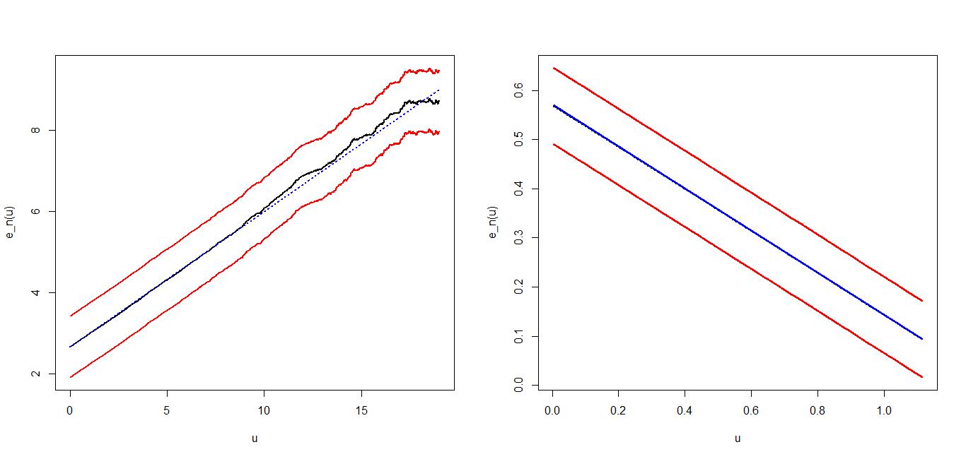
Figure 1. The emef for two generalized Pareto distributions : the left panel concerns the one with the parameters $\xi=0.25,\,\beta=1$ and the right panel concerns the one with the parameters $\xi=-0.75,\,\beta=1$.

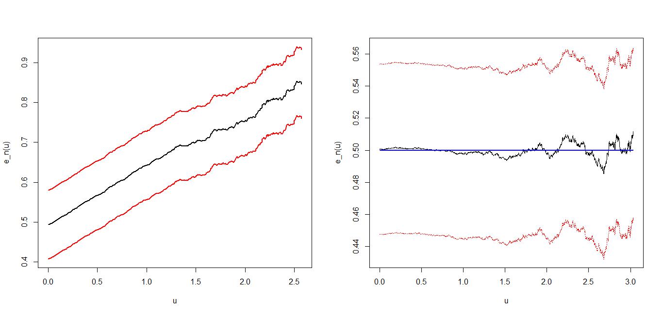
Figure 2. The left panel is the emef for a Pareto distribution with the parameters $\alpha=7$ and $\lambda=3$ and the right panel is the one for an Exponential distribution with the parameter $\lambda=2$.

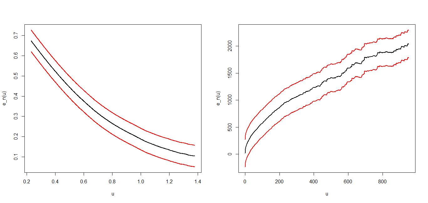
Figure 3. The emef for two Weibull distributions. The left panel concerns the one with the parameters $\beta=1,\,\tau=3.6$ and the right panel concerns the one with the parameters
$\beta=1.5,\,\tau=0.2$.

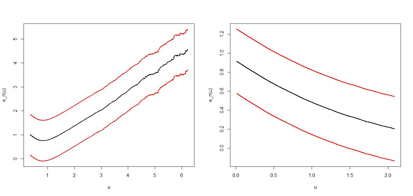
Figure 4. The left panel is the emef for the Burr distribution with the parameters $\alpha=0.5,\,\\ \lambda=0.5,\,\tau=5$ and the right one is the emef for the Gomberz distribution with the parameters $\alpha=1,\,\lambda=0.5$.

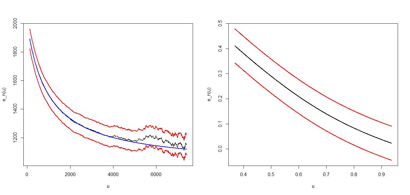
Figure 5. The left panel is the emef for the Gamma distribution with the parameters $\alpha=2,\,\beta=0.001$ and the right one is the emef for the Beta distribution with the parameters $\lambda=7,\beta=2$.

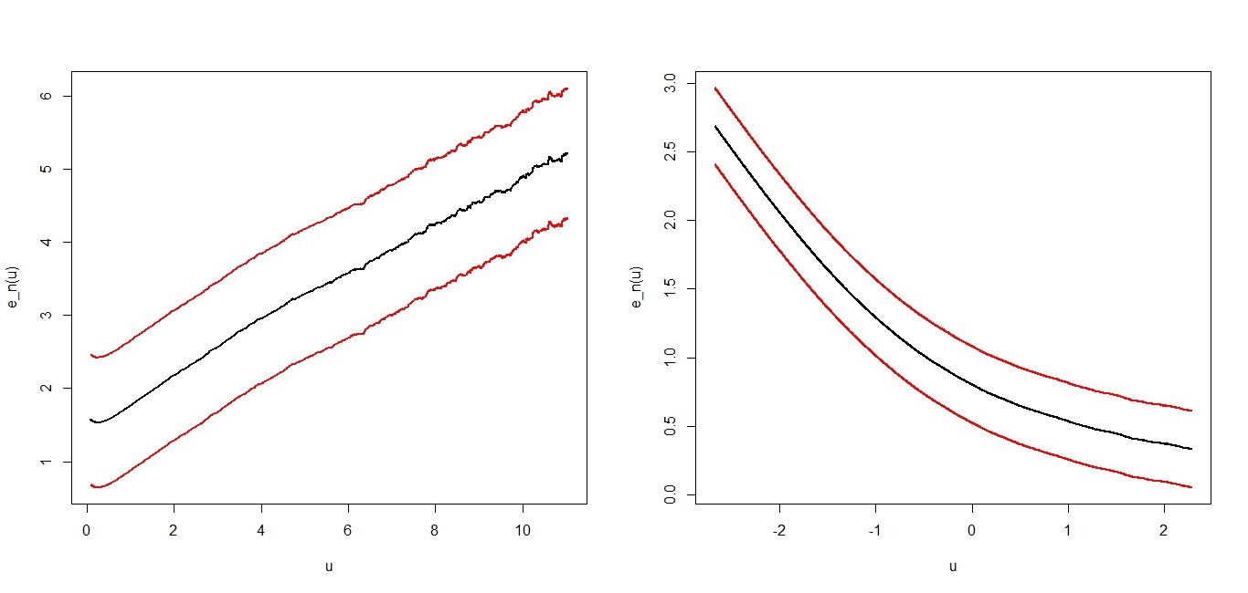
Figure 6. The left panel is the emef for the Lognormal distribution with mean $\mu=0$ and with variance $\sigma^{2}=1$ and the right one is the emef for the Normal distribution with the same parameters.

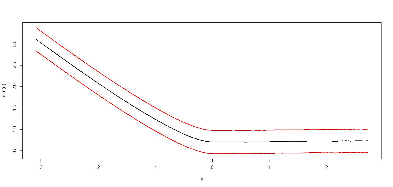
Figure 7. Emef for Laplace distribution with the parameters $\mu=0,\sigma=1,\,\tau=0.5$

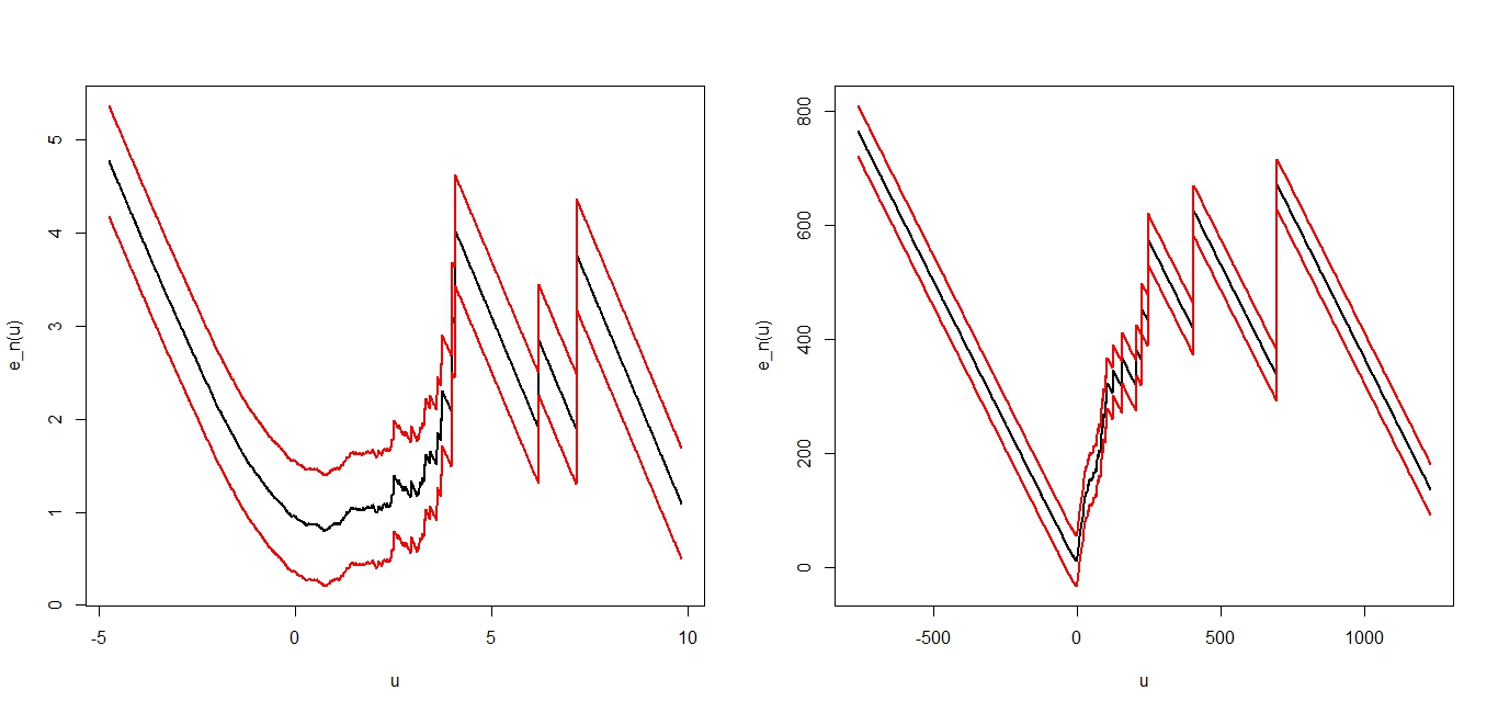
Figure 8. Emef for a $t$ Student with $\nu=5$ degrees of freedom and skewing parameter $\mu=0$ (left panel) and for a Cauchy distribution with location parameter $\mu=0$ and scale parameter $\delta=1$ (right panel).

5.2.2. Generalized hyperbolic models

Next, we consider the emefs for the Gh models. We need some definitions. The Lebesgue density function of the one dimensional Gh is given by

(5.2) $$f_{\lambda,\alpha,\beta,\delta,\mu}(x) = \textbf{a}_{(\lambda,\alpha,\beta,\delta,\mu)}\times\Big{(}\delta^{2}+(x-\mu)^{2}\Big{)}^{(\lambda-\frac{1}{2})/2}e^{\beta(x-u)}\times K_{\lambda-\frac{1}{2}}(\alpha\sqrt{\delta^{2}+(x-\mu)^{2}})$$

where

$$\textbf{a}_{(\lambda,\alpha,\beta,\delta,\mu)}=\frac{(\alpha^{2}-\beta^{2})^{\frac{\lambda}{2}}}{\sqrt{2\pi}\alpha^{(\lambda-\frac{1}{2})}\delta^{\lambda}K_{\lambda}(\delta\sqrt{\alpha^{2}-\beta^{2}})}$$

is a norming constant to make the curve area equal to $1$ and

$$K_{\lambda}(x)=\frac{1}{2}\int_{0}^{\infty}y^{\lambda-1}\exp\Big{(}-\frac{1}{2}x(y+y^{-1})\Big{)}dy,\ \ (x>0)$$

is the modified Bessel function of the third kind with index $\lambda$.

The dependence of the parameters $\lambda,\alpha,\beta,\delta,$ and $\mu$ is as follows: $\alpha>0$ determines the shape, $0\leq|\beta|<\alpha$ the skewness, $\mu\in\mathbb{R}$ is a location parameter and $\delta>0$ serves for scaling. The parameter $\lambda\in\mathbb{R}$ specifies the order $K_{\lambda}$ function Bessel that appears in the Gh density function and is used to obtain different subclasses of Gh distribution.

In the following, we summarise the differents domains of possibilities for the parameters

$$\mbox{If}\ \ \lambda<0,\ \ \big{(}\delta>0,\ \ \,|\beta|\leq\alpha\big{)},$$

$$\mbox{if}\ \ \lambda=0,\ \ \big{(}\delta>0,\ \ \,|\beta|<\alpha\big{)},$$

$$\mbox{if}\ \ \lambda>0,\ \ \big{(}\delta\geq 0,\ \ \,|\beta|<\alpha\big{)}.$$

An important Gh family aspect is that it embraces many special cases such that Hyperbolic ($\lambda=1$), Student-$t\,(\lambda<0$), Variance Gamma ($\lambda>0$), and the Normal Inverse Gaussian (NIG) ($\lambda=-0.5$) distributions.

It nests also Generalized Inverse Gamma (GIG) distribution defined only by the three parameters $\lambda,\alpha,$ and $\beta$. An Inverse Gaussian (IG) distribution is a GIG distribution with $\lambda=-0.5$ and a Gamma ($\Gamma$) distribution is also a GIG distribution with $\beta=0$.

It contains some limiting distributions such as Cauchy distribution with parameters $\mu$ and $\delta$ (obtained for $\lambda=-0.5$ and $\alpha=\beta=0$).

The Gaussian distribution with mean $\mu$ and variance $\sigma^{2}$ are obtained for $\lambda=-0.5$, for $\alpha,\delta\rightarrow\infty$ and $\frac{\delta}{\alpha}\rightarrow\sigma^{2}$.

The Skew-Student $t$ with $\nu$ degrees of freedom is obtained if $\alpha=|\beta|$, then $\nu=-2\lambda>0$.

The Student $t$ distribution is obtained for $\alpha=\beta=0$, $\mu=0$ and $\delta=\sqrt{\nu}$. In the special case of hyperbolic distributions ($\lambda=1),$ we obtain the skewed Laplace distribution for $\delta=0.$

All of these have been used to model financial returns and log-returns.

In table 2, we consider some specific Gh distributions with the superscript $spe$ and limiting distributions with the superscript $lm$. The used parameters are specified and the emef figures corresponding to each choice are displayed.

Distributions	Parameters
	$\lambda$	$\alpha$	$\beta$	$\delta$	$\mu$	Figures
Hyperboliquespe	$1$	$1.5$	$-0.5$	$0.75$	$0.2$
t-Stud.spe	$-2$	$10^{-8}$	$0$	$2$	$0$	Figure 9
Asym. t-Stud.spe	$-1.278$	$0.01186$	$0.01186$	$0.0766$	1.005
	$-1.247$	$0.0148$	$-0.0147$	$0.076$	$1.005$	Figure 10
NIGspe	-0.5	8.03	-1.37	0.051	0.0105
	-0.5	7.6	-1.24	0.052	0.0103	Figure 11
Variance Gammaspe	$2$	0.3	0.1	2	0
$GIG^{spe}$	$5$	$3$	$1$	-	-	Figure 12
$IG$ Inverse Gaussianlm	$0.5$	$1$	$0$	$1$	$0$
Gamma$(\alpha,\beta)^{lm}$	0.5	$4.5\,10^{12}$	$10^{-8}$	-	-	Figure 13
$I\Gamma$ Inverse Gammalm	$-0.5$	$1.9\times 10^{-8}$	$3.1\times 10^{-3}$	-	-
Skew Laplacelm	$1$	$1.1$	$0.1$	$0.001$	$2$	Figure 14
Gaussianlm($3,0.3)$	$-0.5$	$10^{6}$	2	$3\times 10^{5}$	3
Cauchylm $(7,1)$	$-0.5$	$0$	$0$	1	7	Figure 15

Table 2. Specific and limiting GH distributions.

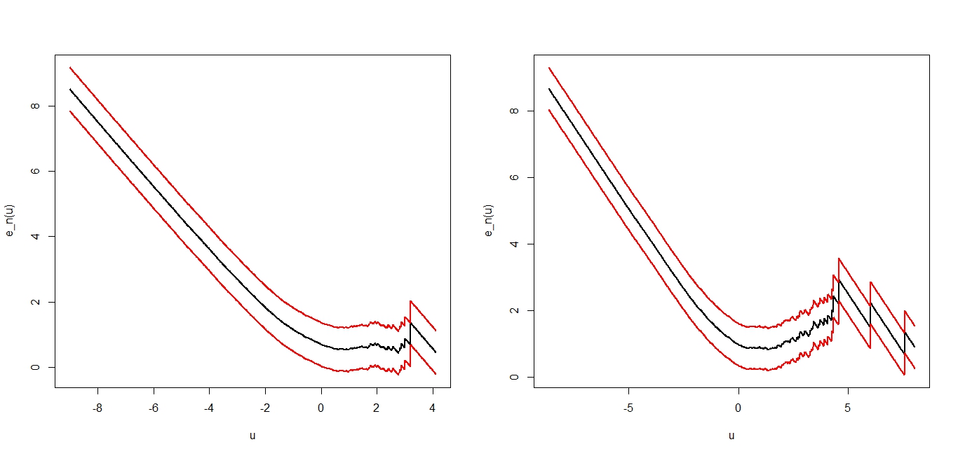
Figure 9. Left panel : Emef for an hyperbolic distribution with the parameters $\lambda=1$, $\alpha=1.5$, $\beta=-0.5$, $\delta=0.75$, $\mu=0.2$. Right panel : Emef for a $t$-student with the parameters $\lambda=-2$, $\alpha=10^{-8}$, $\beta=0$, $\delta=2$, $\mu=0$.

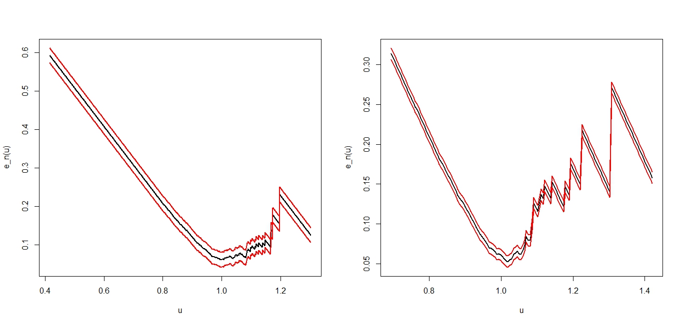
Figure 10. The emef for two $t$-Student distribution. The left panel concerns the one with the parameters $\lambda=-1.278$, $\alpha=0.01186$, $\beta=0.01186$, $\delta=0.0766$, $\mu=1.005$ and the right panel concerns the one with the parameters $\lambda=-1.247$, $\alpha=0.0148$, $\beta=-0.0148$, $\delta=0.07683$, $\mu=1.005$.

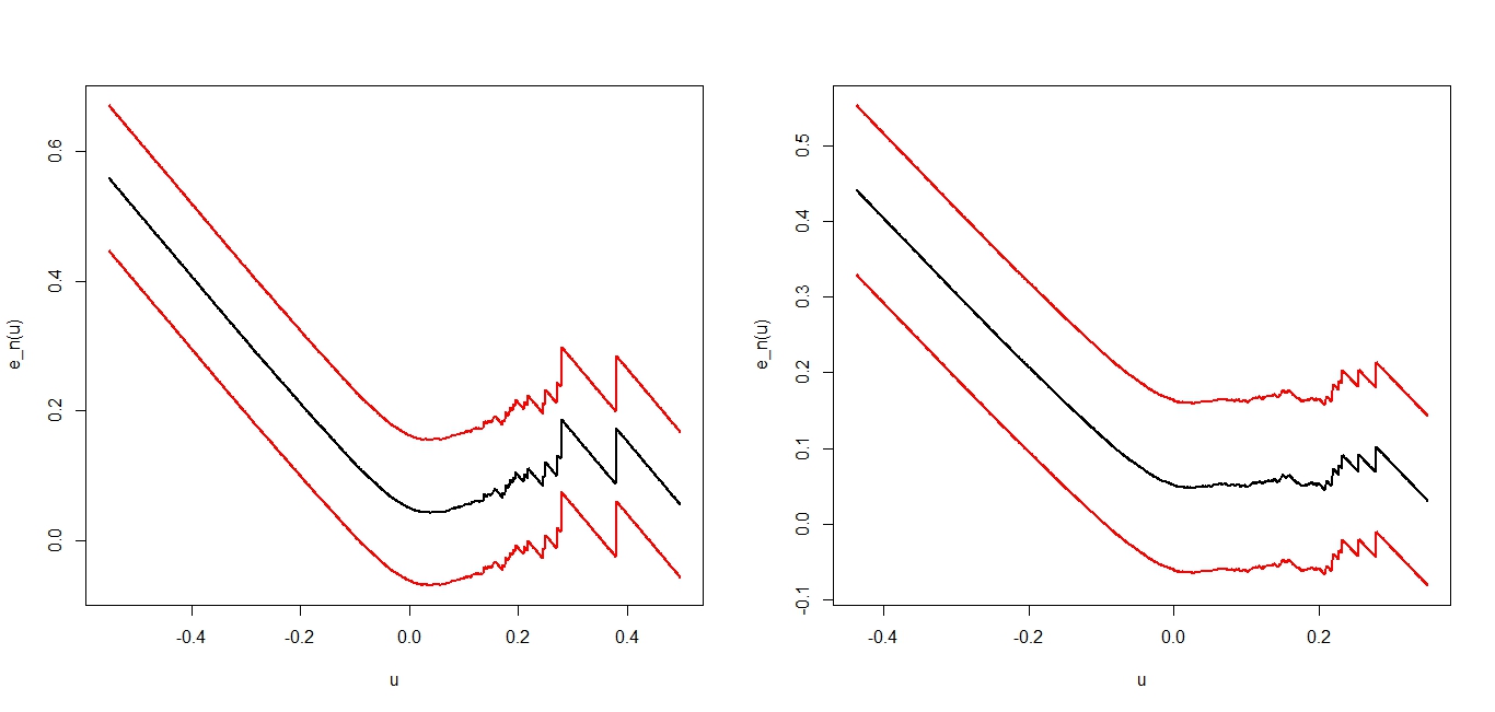
Figure 11. The emef for two Normal Inverse Gaussian distributions. The left panel concerns the one with the parameters $\lambda=-0.5$, $\alpha=8.03$, $\beta=-1.37$, $\delta=0.051$, $\mu=0.0105$ and the right panel concerns the one with the parameters $\lambda=-0.5$, $\alpha=7.6$, $\beta=-1.24$, $\delta=0.052$, $\mu=0.0103$.

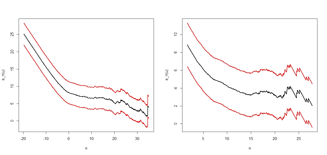
Figure 12. Left panel : the emef for a Variance Gamma distribution with the parameters $\lambda=2$, $\alpha=0.3$, $\beta=0.1$, $\delta=2$, $\mu=0$. Right panel : the emef for a Generalized Inverse Gaussian distribution with the parameters $\lambda=5$, $\alpha=3$, $\beta=1$.

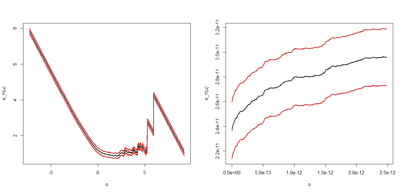
Figure 13. Left panel : the emef for Inverse Gaussian distribution with the parameters $\lambda=0.5$, $\alpha=1$, $\beta=0$, $\delta=1$, $\mu=0$. Right panel : the Emef for a Gamma distribution with the parameters $\lambda=0.5$, $\alpha=4.5\times 10^{12}$, $\beta=10^{-2}$.

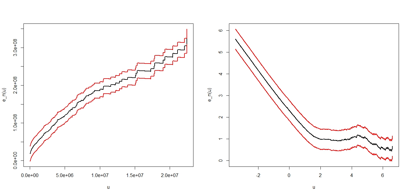
Figure 14. Left panel : the emef for the Inverse Gamma distribution with the parameters
$\lambda=-0.5$, $\alpha=1.9\times 10^{-8}$, $\beta=3.1\times 10^{-3}.$ Right panel : the emef for the Skew Laplace distribution with the parameters $\lambda=1$, $\alpha=1.1$, $\beta=0.1$, $\delta=10^{-3}$, $\mu=2$

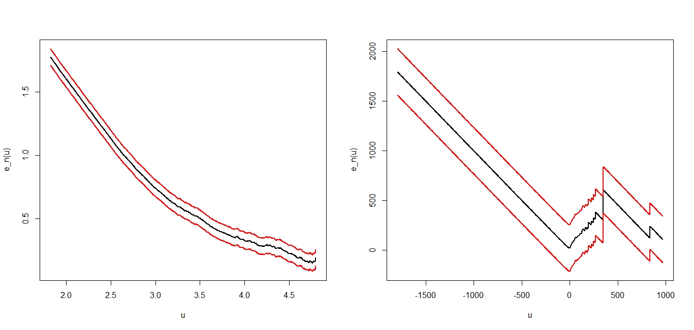
Figure 15. The left panel concerns the emef for the Gaussian distribution with mean $\mu=2$ and variance $\sigma^{2}=0.3$. The right panel concerns the emef for the Cauchy distribution with location parameter $\mu=7$ and scale parameter $\delta=1$.

5.2.3. Graphical test

We are now in a position to use the emef graphs already drawn as tools of goodness of fit.

Emef for Normal Inverse Gaussian (NIG) and $t$-student-distributions are not monotonic function. They decrease and increase like for emef returns data. For this reason, we fit them to both monthly returns and log-returns from Dow Jones data base (see figure 17, figure 19, figure 21, and figure 23).

Dow Jones data base consists of several compagnies like AXP(American Express compagny), CSCO(Cisco Systems), DAX, CAT, IBM and so one. Each one having 5 values : from opening (op) values to closing (cl) values , also minimum (min), maximum (max), and volume (vol) values.

We select AXP and CSCO compagnies and we consider returns and log-returns for their values as showed in the table 3. Then we construct their emef plot and their fitted counterpart.

Estimates parameters and the emef are given in table 4.

Compagnies	Nature	Values	Emef plots
			Real emef	Fitted emef
AXP	Returns	op
		min	Figure 16	Figure 17
	Log-returns.	max
		cl	Figure 18	Figure 19
CSCO	Returns	min
		vol	Figure 20	Figure 21
	Log-returns	op
		max	Figure 22	Figure 23

Table 3. (Fitted) Emef for DAX and CSCO compagnies data.

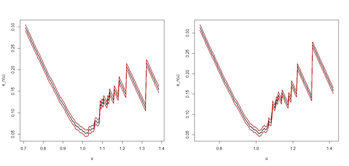
Figure 16. Emef for AXP compagny (monthly data returns). The left panel concerns the opening values and the right one concerns the minimum values.

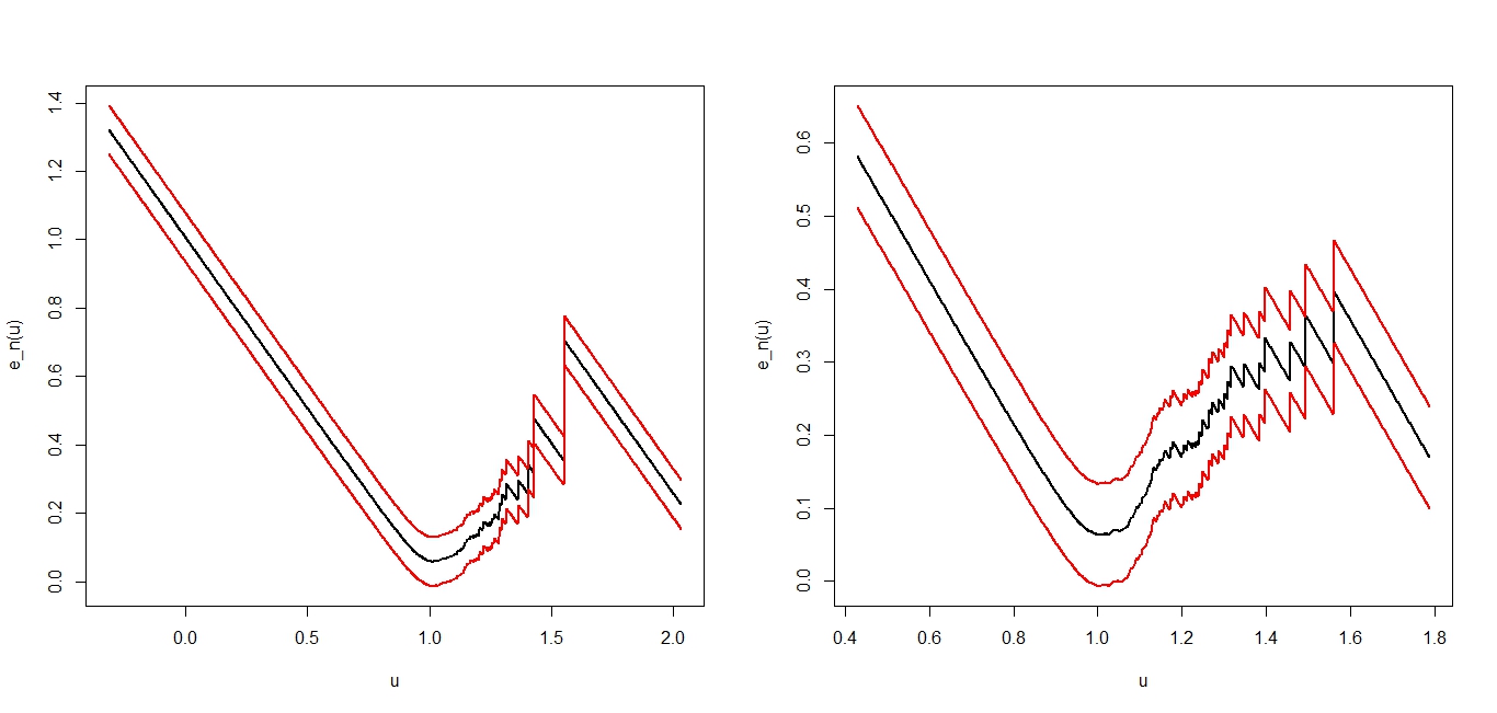
Figure 17. A $t$-Student distribution is fitted to monthly data returns for AXP compagny (see figure 16). The left panel concerns a $t$ distribution with the parameters $\lambda=-1.278,$
$\alpha=0.01186,\beta=0.01186,\delta=0.0766,$ and $\mu=1.005$ fitted to opening values.
The right one concerns a $t$ distribution with the parameters $\lambda=-1.247,\alpha=0.0148$,
$\beta=-0.0148,\delta=0.07683,\mu=1.005$ fitted to minimum values.

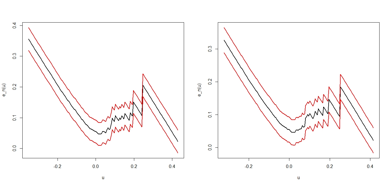
Figure 18. Emef for AXP compagny (monthly data log-returns). The left panel concerns the maximum values and the right panel concerns the closing values.

Comp	Nature	Values	Ghyp estimates parameters
			$\hat{\lambda}$	$\hat{\alpha}$	$\hat{\beta}$	$\widehat{\delta}$	$\hat{\mu}$	Fit.Dist	Figures
AXP	Returns	op.	$-1.278$	$0.01186$	$0.0118$	$0.0766$	$1.005$	$t$-stud
		min.	-1.247	0.0148	-0.0148	0.0768	$1.005$	$t$-stud	Fig. 17
	Log-ret.	max.	-0.5	8.03	-1.37	0.051	0.0105	NIG
		cl.	-0.5	7.6	-1.24	0.052	0.0103	NIG	Fig. 19
CSCO	Returns	min.	-1.24	0.0148	-0.0148	0.0768	1	$t$-Stud.
		vol.	-3.82	4.22	4.22	0.613	0.753	$t$-Stud.	Fig. 21
	Log-ret.	op.	-1.26	0.83	- 0.83	0.07	0	$t$-Stud.
		max.	-1.32	0.85	-0.85	0.076	0	$t$-Stud.	Fig. 23

Table 4. Emef for fitted Gh distributions to DAX and CSCO compagnies data.

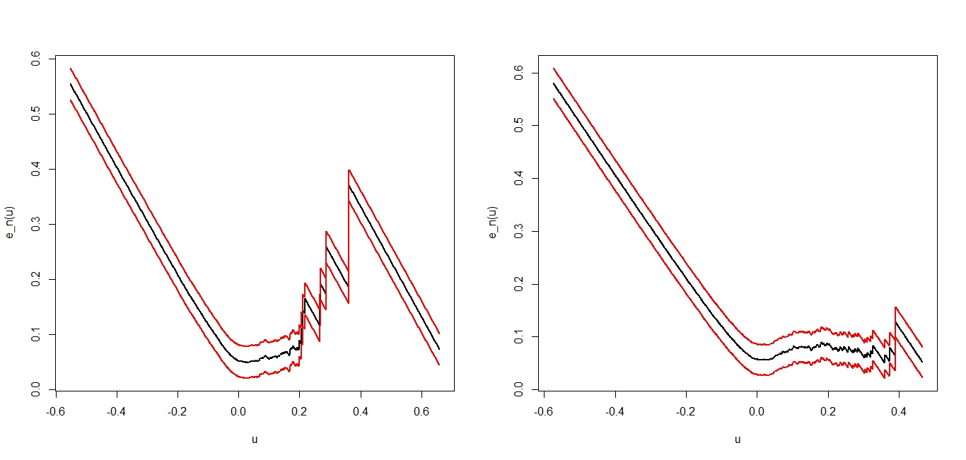
Figure 19. A NIG distribution is fitted to monthly data log-returns for AXP compagny (see Figure 18). The left panel concerns the one with the parameters $\lambda=-0.5,\alpha=8.03,$
$\beta=-1.37,\delta=0.051,\mu=0.0105$ fitted to maximum values. The right panel concerns the one with the parameters $\lambda=-0.5,\alpha=7.6,\beta=-1.24,\delta=0.052,\mu=0.0103$ fitted to closing values.

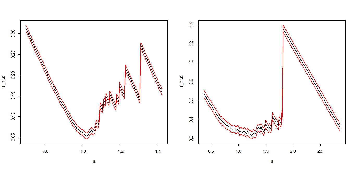
Figure 20. Emef for CSCO compagny (data returns). The left panel concerns monthly minimum values and the right panel concerns monthly volum values.

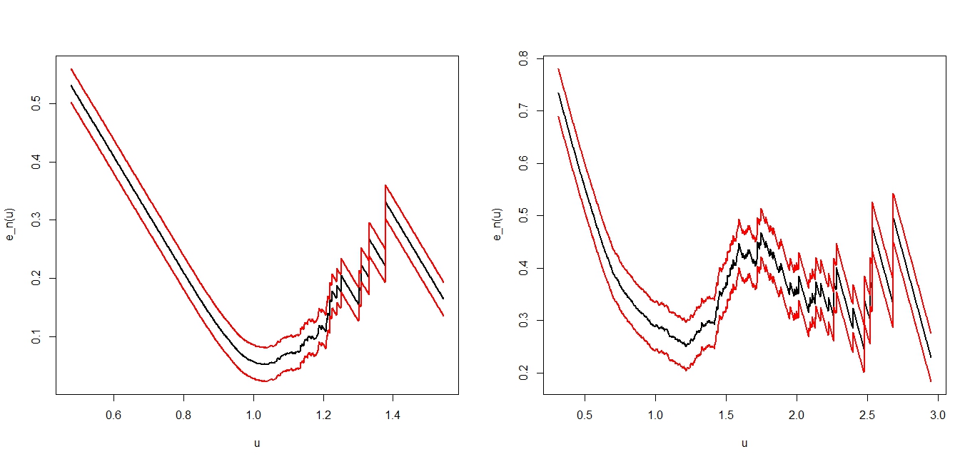
Figure 21. A $t$-student distribution is fitted to monthly data returns for CSCO compagny (see Figure 20). The left panel concerns the one with the parameters $\lambda=-1.24,\,\alpha=0.014,\\ \beta=-0.014,\,\delta=0.076,\,\mu=1$ fitted to minimum values. The right panel concerns the one with the parameters $\lambda=-3.82,\,\alpha=4.22,\beta=4.22,\,\delta=0.613,\,\mu=0.753$ fitted to volume values.

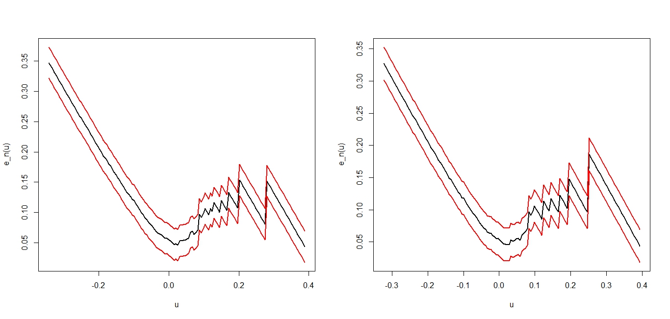
Figure 22. Emef for CSCO compagny (data log-returns). The left panel concerns monthly opening values and the right panel concerns monthly maximum values.

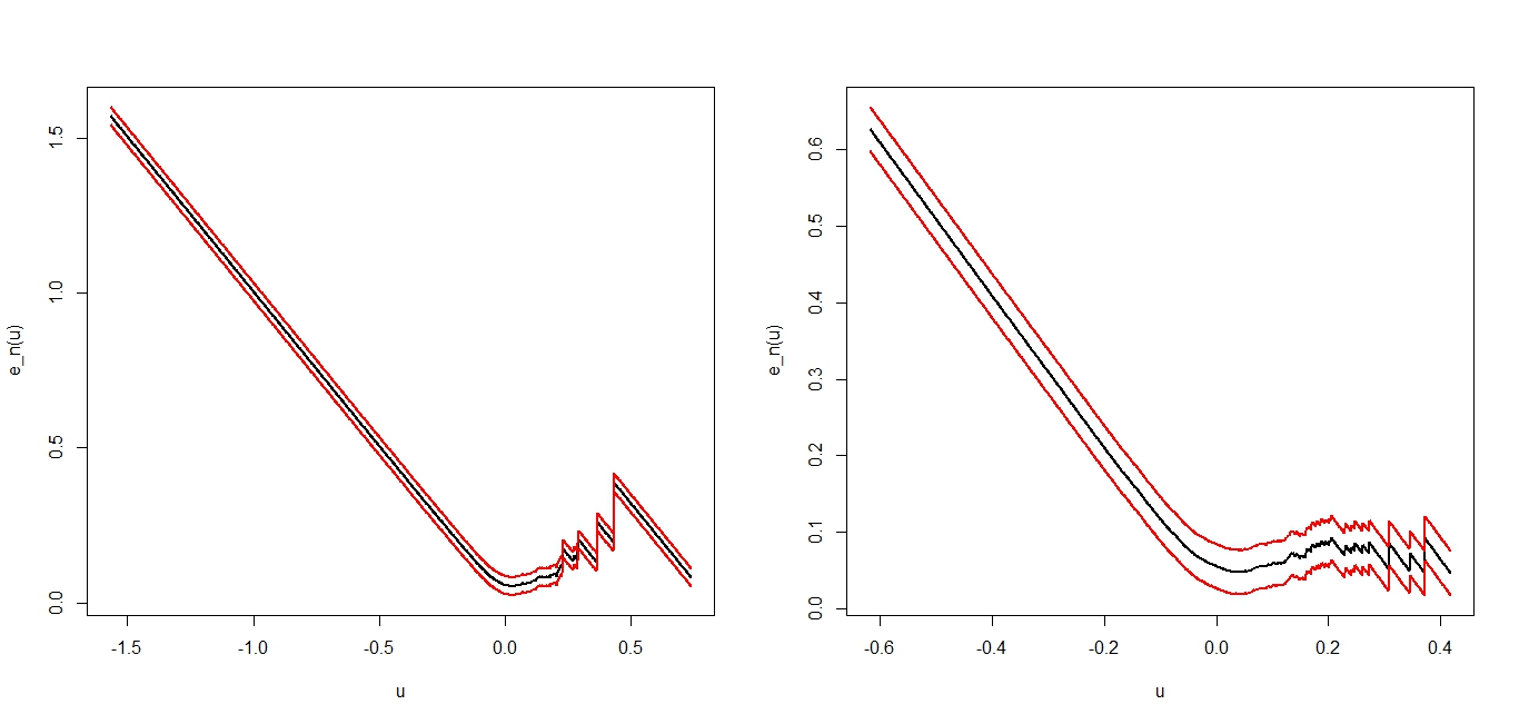
Figure 23. A $t$-student distribution is fitted to monthly data log-returns for CSCO compagny (see Figure 22). The left panel concerns the one with the parameters $\lambda=-1.26,\\ \alpha=0.83,\,\beta=-0.83,\,\delta=0.07,\,\mu=0$ fitted to opening values. The right panel concerns the one with the parameters $\lambda=-1.32,\,\alpha=0.85,\beta=-0.85,\,\delta=0.076,\,\mu=0$ fitted to maximum values.

5.2.4. Commentaries

In view of figure 10 and figure 17 we can say that $t$ studient distribution fits well opening and minimum values return for the American Express compagny AXP, whereas $NIG$ distribution fits well maximum and closing log-returns values for the Cysco System compagny CSCO in view of figure 11 and figure 19.

6. Conclusion

In this paper we have established an asymptotic confidence bands for the mean excess function by using functional process approach. Then we applied these bands for fitting Gh distributions to Dowjones financial data. It is a known fact that these ones fit well financial data since they embrace major part of classic distributions.

We remarked that Student and $NIG$ distributions are good candidates for fitting returns and log-returns data showing their semi-heavy tails.

7. Appendix

7.1.
Moment computations

 
Let $Z_{1},...,Z_{n},$ $n$ i.i.d centered random variables defined on the same probability space with common variance $\mathbb{E}(Z_{i}^{2})=\kappa_{1}$ and common fourth moment  $\mathbb{E}(Z_{i}^{4})=\kappa_{2}>0$. We have

(7.1) $$\displaystyle\mathbb{E}\big{[}T(n,u,\delta)\big{]}^{4} = \mathbb{E}\Big{(}Z_{1}+Z_{2}+\ldots Z_{n}\Big{)}^{4}$$

$$= \mathbb{E}\Big{(}\sum_{k=1}^{n}Z_{k}^{4}+6\sum_{1\leq i<j\leq n}Z_{i}^{2}Z_{j}^{2}\Big{)}$$

$$= \sum_{k=1}^{n}\mathbb{E}(Z_{k}^{4})+6\sum_{1\leq i<j\leq n}\mathbb{E}(Z_{i}^{2}Z_{j}^{2})$$

since, for distinct $i$, $j$, $k$ and $l$,

$$\mathbb{E}(Z_{i}Z_{j}^{3})=\mathbb{E}(Z_{i}Z_{j}^{2}Z_{k})=\mathbb{E}(Z_{i}Z_{j}Z_{k}Z_{l})=0,$$

by using independence plus the fact that $\mathbb{E}(Z_{i})=0$.
Using independence again,

$$\mathbb{E}(Z_{i}^{2}Z_{j}^{2})=\mathbb{E}(Z_{i}^{2})\mathbb{E}(Z_{j}^{2})=\kappa_{1}^{2}\ \ \mbox{for}\ \ i\neq j.$$

We obtain $\displaystyle\sum_{1\leq i<j\leq n}\mathbb{E}(Z_{i}^{2}Z_{j}^{2})=\frac{n(n-1)}{2}\kappa_{1}^{2}$ since the number of possible couples $(i,j)$ of integers such that $1\leq i<j\leq n$, is $\displaystyle\binom{n}{2}=\frac{n(n-1)}{2}$. Hence from (7.1), we deduce that

$$\mathbb{E}\big{[}T(n,u,\delta)\big{]}^{4}=n\kappa_{2}+3n(n-1)\kappa_{1}^{2}.$$

$\square$

7.2.
Proofs of the uniform asymptotic consistency bounds.

7.2.1. Talagrand bounds

We begin to recall the Talagrand bounds and a device of Einmahl and Mason on how to apply it.
Before going any further, we recall that a class of measurable real valued functions $\mathcal{F}$ is said to be a pointwise measurable class if there exists a countable subclass $\mathcal{F}_{0}\$ of $\mathcal{F}$ such as, for any function $f$ in $\mathcal{F}$, we can find a sequence of functions $\{f_{m}\}_{m\geq 0}$ in $\mathcal{F}_{0}$ for which $f_{m}(x)\rightarrow f(x)\ \ \mbox{as}\ \ m\rightarrow\infty$ , $x\in\mathbb{R}$. (See Example 2.3.4 in [10].
Further, let $\xi_{1},\xi_{2},\ldots$ be a sequence of independent Rademacher random variables independent of $X_{1},X_{2},\ldots,$ and $\mathbb{G}_{m}$ be the functional empirical process indexed by the class of functions $\mathcal{F}$.

The following inequality is essentially due to Talagrand (1994) (see [8]).

Inequality. Let $\mathcal{F}$ be a pointwise measurable class of functions satisfying for some
$0<M<\infty,\,\|f\|_{\infty}\leq M,\,\ \ f\in\mathcal{F},$ .
Then for all $t>0$ we have,

$$\mathbb{P}\Big{\{}\max_{1\leq m\leq n}\|\sqrt{m}\mathbb{G}_{m}\|_{\mathcal{F}}\geq A_{1}\Big{(}\mathbb{E}\Big{\|}\sum_{i=1}^{n}\xi_{i}f(X_{i})\Big{\|}_{\mathcal{F}}+t\Big{)}\Big{\}}$$

(7.2) $$\ \ \ \ \ \ \ \ \ \ \ \ \ \ \leq\ \ 2\big{(}\exp(-A_{2}\,t^{2}/n\sigma_{\mathcal{F}}^{2})+\exp(-A_{2}\,t/M)\big{)},$$

where $\sigma_{\mathcal{F}}^{2}=\sup_{f\in\mathcal{F}}Var(f(X))$ and $A_{1},A_{2}$ are universal constants.

And the lemma below of Einmahl and Mason [9] is very helpful for obtaining bounds on this quantity, when the class $\mathcal{F}$ has a polynomial covering number.

Assume that there exists a finite valued measurable function $G$, called an envelope function, which satisfies for all $\displaystyle x\in\mathbb{R},\,G(x)\geq\sup_{f\in\mathcal{F}}\left|f(x)\right|$. We define for $0<\epsilon<1$

$$N(\varepsilon,\mathcal{F}):=\sup_{Q}N\Big{(}\epsilon\sqrt{Q(G^{2})},\mathcal{F},d_{Q}\Big{)}$$

where the supremum is taken over all probability measures $Q$ on $\mathbb{R}$ for which $0<Q(G^{2}):=\int G^{2}(y)Q(dy)<\infty$ and $d_{Q}$ is the $L_{2}(Q)-$metric. As usual, $N(\epsilon,\mathcal{F},d_{Q}$) is the minimal number of balls $\{g:d_{Q}(g,f)<\epsilon\}$ of $d_{Q}-$radius $\epsilon$ needed to cover $\mathcal{F}$. Here is the device of Einmahl and Mason [9].

Lemma 3.

(Einmahl - Mason [9]) Let $\mathcal{F}$ be a pointwise measurable class of bounded functions such that for some constants $\beta>0,\,\nu>0,\,C>1,\,\sigma\leq 1/(8C)$ and function $G$ as above, the following four conditions hold:

1. $\mathbb{E}\Big{[}G^{2}(X)\Big{]}\leq\beta^{2};$

2. $N(\epsilon,\mathcal{F})\leq C\varepsilon^{-\nu},\ \ 0<\epsilon<1$;

3. $\displaystyle\sigma_{0}^{2}:=\sup_{f\in\mathcal{F}}\mathbb{E}\Big{[}f^{2}(X)\Big{]}\leq\sigma^{2};$

4. $\displaystyle\sup_{f\in\mathcal{F}}\|f\|_{\infty}\leq\frac{1}{2\sqrt{\nu+1}}\sqrt{n\sigma^{2}/\log(\beta\vee 1/\sigma)}.$

Then we have for some absolute constant $A$,

(7.3) $$\mathbb{E}\Big{\|}\sum_{i=1}^{n}\xi_{i}f(X_{i})\Big{\|}_{\mathcal{F}}\leq A\sqrt{\nu n\sigma^{2}\log(\beta\vee 1/\sigma)}.$$

7.2.2. APPLICATION

Put $\ell_{u}(x)=\ell(x)\mathbb{I}_{(x>u)}$, with $\ell(x)=1$ or $\ell(x)=x$, and let $\mathcal{F}=\{\ell_{u},u\in I\}.$
$\mathcal{F}$ is pointwise measurable since it suffices to take $\mathcal{F}_{0}=\{\ell_{u},u\in I\cap\mathbb{Q}\},$ where $\mathbb{Q}$ is the set of irrationnal numbers.

Next $G=\max(\left|\ell(u_{0})\right|,\left|\ell(u_{1})\right|)=M>0$ is an envelope of $\mathcal{F}$ since we have

$$\sup_{u\in I}|\ell_{u}(x)|\leq|\ell(x)|\leq\max(\left|\ell(u_{0})\right|,\left|\ell(u_{1})\right|),\quad\forall\,u_{0}\leq x\leq u_{1}.$$

Remark that if $\ell(x)=1$ then $M=1$ and if $\ell(x)=x$ then $M=\max(|u_{0}|,|u_{1}|).$
We have $\displaystyle\sigma_{\mathcal{F}}^{2}=\sup_{f\in\mathcal{F}}Var(f(X))\leq M^{2}.$
So we may use Talagrand’s inequality : it remains to check points of Lemma 3:
Points (A.1) and (A.3) are obvious with $\beta=M=\sigma.$
To check (A.2), consider any probability $Q$ on $\mathbb{R}.$ We get for $(u,v)\in I^{2},u\leq v,$

(7.4) $$d_{Q}^{2}(\ell_{u},\ell_{v})=\int(\ell_{u}-\ell_{v})^{2}(x)dQ(x)\leq M^{2}Q([u,v]).$$

By a classical result in probability in $\mathbb{R}$, for any given $0<\varepsilon<1,$ we may cover $[u_{0},u_{1}]$ by at most
$\displaystyle m=\lceil\frac{u_{1}-u_{0}}{\varepsilon}\rceil$ sub-intervals $\displaystyle[s_{i-1},s_{i}]$ such that $Q([s_{i-1},s_{i}])<\varepsilon^{2},\ \ i=1,\ldots,m.$
($\lceil x\rceil$ stands for the smallest positive integer greater than or equal to $x$).
Let $C=(m+1)\varepsilon$, we have $m<C\varepsilon^{-1}$.

For any $u\in[u_{0},u_{1}]$, there exists $i\in\{1,\ldots,m\}$ such as $s_{i-1}\leq u\leq s_{i}$ with $Q([u,s_{i}])<\varepsilon^{2}$, so the corresponding $\ell_{u}\in\mathcal{F}$ is such that

$$d_{Q}(\ell_{u},\ell_{s_{i}})<\varepsilon M=\varepsilon\sqrt{Q(G^{2})}\ \ \ \mbox{from \eqref{ent}}.$$

To finish $m=N\Big{(}\epsilon\sqrt{Q(G^{2})},\mathcal{F},d_{Q}\Big{)}<C\varepsilon^{-1}$ and

$$N(\epsilon,\mathcal{F})=\sup_{Q}N\Big{(}\epsilon\sqrt{Q(G^{2})},\mathcal{F},d_{Q}\Big{)}\leq C\varepsilon^{-1}.$$

Now we take $\beta^{2}=\sigma^{2}=\max(2,\max(\left|\ell(u_{0})\right|,\left|\ell(u_{1})\right|)=M_{1}.$
Finally for

$$n\geq\frac{8M^{2}\log M_{1}}{M_{1}^{2}},$$

we have

(7.5) $$\mathbb{E}\Big{\|}\sum_{i=1}^{n}\xi_{i}g(X_{i})\Big{\|}_{\mathcal{F}}\leq C_{\mathcal{F}}\sqrt{n},$$

where $\displaystyle C_{\mathcal{F}}=A\,M_{1}\sqrt{\log M_{1}},$ since all the points of the Lemma 3 are checked.

Now we are going to apply the inequality (7.2.1) first for the class of functions

$$\mathcal{F}_{1}=\{\ell_{u}(x)=g_{u}(x),u\in I\}.$$

In this case $M_{1}=2$ since $\ell(x)=1$, for any $u_{0}\leq x\leq u_{1}$, and

$$\mathbb{E}\Big{\|}\sum_{i=1}^{n}\xi_{i}g_{u}(X_{i})\Big{\|}_{\mathcal{F}_{1}}=D_{n,1}\leq C_{\mathcal{F}_{1}}\sqrt{n},\ \ \mbox{where}\ \ C_{\mathcal{F}_{1}}=2A\sqrt{\log 2}.$$

Let $\varepsilon>0,\,n_{1}\geq 2\log 2$ and $t_{0}$ such that

$$\exp\Big{(}\frac{-A_{2}t_{0}^{2}}{n_{1}}\Big{)}\leq\frac{\varepsilon}{8},\ \ \mbox{and}\ \ \exp\Big{(}-A_{2}t_{0}\Big{)}\leq\frac{\varepsilon}{8}\ \ \mbox{and}\ \ \ t_{0}<\sqrt{n_{1}}.$$

(Remind that $\sigma_{\mathcal{F}}^{2}=1$.)
Then

$$\displaystyle\mathbb{P}\Big{\{}\max_{1\leq m\leq n}\|\sqrt{m}\mathbb{G}_{m}\|_{\mathcal{F}_{1}}\geq A_{1}\Big{(}\mathbb{E}\Big{\|}\sum_{i=1}^{n}\xi_{i}g_{u}(X_{i})\Big{\|}_{\mathcal{F}_{1}}+\,t_{0}\Big{)}\Big{\}}\leq\varepsilon/2.$$

So for $n\geq n_{1},$ we arrive at

$$\mathbb{P}\Big{(}\left|\mathbb{P}_{n}(g_{u})-\mathbb{P}_{X}(g_{u})\right|<\frac{A_{1}(D_{n,1}+t_{0})}{n},u\in I\Big{)}>1-\varepsilon/2.$$

As $t_{0}/\sqrt{n}<\sqrt{n_{1}}/\sqrt{n}\leq 1$, we obtain

$$\frac{A_{1}(D_{n,1}+t_{0})}{n}\leq\frac{A_{1}C_{\mathcal{F}_{1}}\sqrt{n}+A_{1}\sqrt{n}}{n}=\frac{A_{1}C_{\mathcal{F}_{1}}+A_{1}}{\sqrt{n}}=\frac{D_{1}}{\sqrt{n}},$$

thus

(7.6) $$\mathbb{P}\Big{(}\left|\mathbb{P}_{n}(g_{u})-\mathbb{P}_{X}(g_{u})\right|<\frac{D_{1}}{\sqrt{n}},u\in I\Big{)}>1-\varepsilon/2$$

where $D_{1}=2A\,A_{1}\sqrt{\log 2}+A_{1}$.

Let us use the same method, for the class of functions

$$\mathcal{F}_{2}=\{\ell_{u}(x)=f_{u}(x),u\in I\}.$$

In this case $M_{1}=\max(2,\max(|u_{0}|,|u_{1}|))$ since $\ell(x)=x,$ for any $u_{0}\leq x\leq u_{1}$, and

$$\mathbb{E}\Big{\|}\sum_{i=1}^{n}\xi_{i}f_{u}(X_{i})\Big{\|}_{\mathcal{F}_{2}}=D_{n,2}\leq C_{\mathcal{F}_{2}}\sqrt{n},\mbox{where}\ \ C_{\mathcal{F}_{2}}=AM_{1}\sqrt{\log M_{1}}.$$

Let $\displaystyle n_{2}\geq\frac{8M^{2}\log M_{1}}{M_{1}^{2}}$ and $t_{0}$ such that

$$\exp\Big{(}\frac{-A_{2}t_{0}^{2}}{n_{2}}\Big{)}\leq\frac{\varepsilon}{8}\ \ \mbox{and}\ \ \exp\Big{(}-A_{2}t_{0}\Big{)}\leq\frac{\varepsilon}{8}\ \ \mbox{and}\ \ t_{0}<\sqrt{n_{2}}.$$

Then

$$\displaystyle\mathbb{P}\Big{\{}\max_{1\leq m\leq n}\|\sqrt{m}\mathbb{G}_{m}\|_{\mathcal{F}_{2}}\geq A_{1}\Big{(}\mathbb{E}\Big{\|}\sum_{i=1}^{n}\xi_{i}f_{u}(X_{i})\Big{\|}_{\mathcal{F}_{2}}+t_{0}\Big{)}\Big{\}}\leq\varepsilon/2.$$

So for $n\geq n_{2},$ we deduce that

$$\mathbb{P}\Big{(}\left|\mathbb{P}_{n}(f_{u})-\mathbb{P}_{X}(f_{u})\right|<\frac{A_{1}(D_{n,2}+t_{0})}{n},u\in I\Big{)}>1-\varepsilon/2.$$

As $t_{0}/\sqrt{n}<\sqrt{n_{1}}/\sqrt{n}\leq 1$, we obtain

$$\frac{A_{1}(D_{n,2}+t_{0})}{n}\leq\frac{A_{1}C_{\mathcal{F}_{2}}\sqrt{n}+A_{1}\sqrt{n}}{n}=\frac{A_{1}C_{\mathcal{F}_{2}}+A_{1}}{\sqrt{n}}=\frac{D_{2}}{\sqrt{n}},$$

thus

(7.7) $$\mathbb{P}\Big{(}\left|\mathbb{P}_{n}(f_{u})-\mathbb{P}_{X}(f_{u})\right|<\frac{D_{2}}{\sqrt{n}},u\in I\Big{)}>1-\varepsilon/2,$$

where $D_{2}=A\,A_{1}\,M_{1}\sqrt{\log M_{1}}+A_{1}$.

Now we use again (2.3) :

$$|{e}_{n}(u)-e(u)|\leq|\mathbb{P}_{n}(f_{u})-\mathbb{P}_{X}(f_{u})|\times|\mathbb{P}_{n}(g_{u})|^{-1}\ +\ |\mathbb{P}_{X}(f_{u})|\times\frac{|\mathbb{P}_{n}(g_{u})-\mathbb{P}_{X}(g_{u})|}{|\mathbb{P}_{n}(g_{u})\mathbb{P}_{X}(g_{u})|}.$$

For $u_{0}\leq u\leq u_{1}$, we get

$$0<\overline{F}(u_{1})-\frac{D_{1}}{\sqrt{n}}\leq\mathbb{P}_{X}(g_{u})-\frac{D_{1}}{\sqrt{n}}<\mathbb{P}_{n}(g_{u})<\mathbb{P}_{X}(g_{u})+\frac{D_{1}}{\sqrt{n}}$$

with a probability greater than (w.p.g.t) $1-\varepsilon/2$ and thus

$$|\mathbb{P}_{n}(g_{u})|^{-1}<\Big{(}\overline{F}(u_{1})-\frac{D_{1}}{\sqrt{n}}\Big{)}^{-1}\ \ \mbox{{w.p.g.t}}\ \ 1-\varepsilon/2$$

so we obtain

$$\mathbb{P}\left(|\mathbb{P}_{n}(f_{u})-\mathbb{P}_{X}(f_{u})|\times|\mathbb{P}_{n}(g_{u})|^{-1}<\frac{D_{2}}{\sqrt{n}}\times\Big{(}\overline{F}(u_{1})-\frac{D_{1}}{\sqrt{n}}\Big{)}^{-1},u\in I\right)$$

$$\ \ \ \ \ \ \ \ \ \ \ \ \ \ \ \ \geq\mathbb{P}\Big{(}\left|\mathbb{P}_{n}(f_{u})-\mathbb{P}_{X}(f_{u})\right|<\frac{D_{2}}{\sqrt{n}},u\in I\Big{)}>1-\varepsilon/2,$$

thus

(7.8) $$\mathbb{P}\left(|\mathbb{P}_{n}(f_{u})-\mathbb{P}_{X}(f_{u})|\times|\mathbb{P}_{n}(g_{u})|^{-1}<\frac{D_{2}}{\sqrt{n}}\times\Big{(}\overline{F}(u_{1})-\frac{D_{1}}{\sqrt{n}}\Big{)}^{-1},u\in I\right)>1-\varepsilon/2.$$

From the following inequalities :

$$\begin{cases}\displaystyle|\mathbb{P}_{n}(g_{u})|^{-1}\leq\Big{(}\overline{F}(u_{1})-\frac{D_{1}}{\sqrt{n}}\Big{)}^{-1},\ \ \mbox{{w.p.g.t}}\ \ 1-\varepsilon/2,\\ |\mathbb{P}_{X}(g_{u})|^{-1}\leq\overline{F}(u_{1})^{-1},\\ |\mathbb{P}_{X}(f_{u})|\leq\mathbb{E}|X|,\end{cases}$$

and by the same manner, we obtain

$$\mathbb{P}\left(|\mathbb{P}_{X}(f_{u})|\times\frac{|\mathbb{P}_{n}(g_{u})-\mathbb{P}_{X}(g_{u})|}{|\mathbb{P}_{n}(g_{u})\mathbb{P}_{X}(g_{u})|}<\frac{D_{1}}{\sqrt{n}}\times\mathbb{E}|X|\times\Big{(}\overline{F}(u_{1})(\overline{F}(u_{1})-\frac{D_{1}}{\sqrt{n}})\Big{)}^{-1},u\in I\right)$$

$$\ \ \ \ \ \ \ \ \ \ \ \ \ \ \ \ \geq\mathbb{P}\Big{(}\left|\mathbb{P}_{n}(g_{u})-\mathbb{P}_{X}(g_{u})\right|<\frac{D_{1}}{\sqrt{n}},u\in I\Big{)}>1-\varepsilon/2\,,$$

thus

(7.9) $$\mathbb{P}\left(|\mathbb{P}_{X}(f_{u})|\times\frac{|\mathbb{P}_{n}(g_{u})-\mathbb{P}_{X}(g_{u})|}{|\mathbb{P}_{n}(g_{u})\mathbb{P}_{X}(g_{u})|}<\frac{D_{1}}{\sqrt{n}}\times\mathbb{E}|X|\times\Big{(}\overline{F}(u_{1})(\overline{F}(u_{1})-\frac{D_{1}}{\sqrt{n}})\Big{)}^{-1}\right)>1-\varepsilon/2$$

By combining (7.8) and (7.9), we obtain

$$\mathbb{P}\left(|\mathbb{P}_{n}(g_{u})|^{-1}\times\left|\mathbb{P}_{n}(f_{u})-\mathbb{P}_{X}(f_{u})\right|\geq\frac{D_{2}}{\sqrt{n}}\times\Big{(}\overline{F}(u_{1})-\frac{D_{1}}{\sqrt{n}}\Big{)}^{-1},u\in I\right)$$

$$\ \ \ \ \ \ \ \ \ \ \ \ \ \ \ \ \ +\ \ \ \mathbb{P}\left(|\mathbb{P}_{X}(f_{u})|\times\frac{|\mathbb{P}_{n}(g_{u})-\mathbb{P}_{X}(g_{u})|}{|\mathbb{P}_{n}(g_{u})\mathbb{P}_{X}(g_{u})|}\geq\frac{D_{1}}{\sqrt{n}}\times\mathbb{E}|X|\times\Big{(}\overline{F}(u_{1})(\overline{F}(u_{1})-\frac{D_{1}}{\sqrt{n}})\Big{)}^{-1}\right)$$

$$\ \ \ \ \ \ \ \ \ \ \ \ \ \ \ \ \ \leq\ \ \ \frac{\varepsilon}{2}\ \ \ \ +\ \ \ \ \frac{\varepsilon}{2}\ \ \ \ \leq\ \ \ \ \varepsilon\,.$$

This gives

$$\mathbb{P}(|e_{n}(u)-e(u)|\geq\frac{E_{n}}{\sqrt{n}})\leq\varepsilon\ \ \ \mbox{where}\ \ \ E_{n}=\frac{1}{\overline{F}(u_{1})-D_{1}/\sqrt{n}}\Big{(}D_{2}+\frac{D_{1}\times\mathbb{E}|X|}{\overline{F}(u_{1})}\Big{)}.$$

Finally we conclude by :

$$\mathbb{P}\Big{(}e_{n}(u)-\frac{E_{n}}{\sqrt{n}}<e(u)<e_{n}(u)+\frac{E_{n}}{\sqrt{n}},u\in I\Big{)}>1-\varepsilon$$

for any $\varepsilon>0$, any $n\geq n_{0}$ with

$$E_{n}=\frac{1}{\overline{F}(u_{1})-D_{1}/\sqrt{n}}\Big{(}D_{2}+\frac{D_{1}\times\mathbb{E}|X|}{\overline{F}(u_{1})}\Big{)}\ \ \ \mbox{and}\ \ \ \ \ \left\{\begin{array}[]{l}\displaystyle D_{1}=2AA_{1}\sqrt{\log 2}+A_{1}\cr\displaystyle D_{2}=A\,A_{1}\,M_{1}\sqrt{\log M_{1}}+A_{1},\cr M_{1}=\max(2,\max(|u_{0}|,|u_{1}|))\cr\end{array}\right.$$

$\square$