Probing the Physical Properties of $z=$ 4.5 Lyman Alpha Emitters with Spitzer

Keely D. Finkelstein¹¹affiliation: Department of Astronomy, The University of Texas at Austin, 2515 Speedway, Stop C1400, Austin, TX 78712, USA , Steven L. Finkelstein¹¹affiliation: Department of Astronomy, The University of Texas at Austin, 2515 Speedway, Stop C1400, Austin, TX 78712, USA , Vithal Tilvi²²affiliation: George P. and Cynthia Woods Mitchell Institute for Fundamental Physics and Astronomy, Department of Physics and Astronomy, Texas A&M University, College Station, TX 77843-4242, USA , Sangeeta Malhotra³³affiliation: School of Earth and Space Exploration, Arizona State University, Tempe, AZ 85287, USA , James E. Rhoads³³affiliation: School of Earth and Space Exploration, Arizona State University, Tempe, AZ 85287, USA , Norman A. Grogin⁴⁴affiliation: Space Telescope Science Institute, 3700 San Martin Drive, Baltimore, MD 21218, USA , Norbert Pirzkal⁴⁴affiliation: Space Telescope Science Institute, 3700 San Martin Drive, Baltimore, MD 21218, USA , Arjun Dey⁵⁵affiliation: National Optical Astronomy Observatory, 950 North Cherry Ave., Tucson, AZ 85719, USA ⁶⁶affiliation: Radcliffe Institute for Advanced Study, Byerly Hall, Harvard University, 10 Garden St., Cambridge, MA 02138, USA , Buell T. Jannuzi⁵⁵affiliation: National Optical Astronomy Observatory, 950 North Cherry Ave., Tucson, AZ 85719, USA , Bahram Mobasher⁷⁷affiliation: Department of Physics and Astronomy, University of California, Riverside, CA 92521, USA , Sabrina Pakzad⁸⁸affiliation: Gemini Observatory, 670 N. A’ohoku Place, Hilo, HI 96720, USA , Brett Salmon²²affiliation: George P. and Cynthia Woods Mitchell Institute for Fundamental Physics and Astronomy, Department of Physics and Astronomy, Texas A&M University, College Station, TX 77843-4242, USA , and Junxian Wang⁹⁹affiliation: CAS Key laboratory for Research in Galaxies and Cosmology, Dept. of Astronomy, University of Science and Technology of China, Hefei, Anhui 230026, China

Abstract

We present the results from a stellar population modeling analysis of a sample of 162 $z=$ 4.5, and 14 $z=$ 5.7 Lyman alpha emitting galaxies (LAEs) in the Bo $\ddot{\textrm{o}}$ tes field, using deep Spitzer/IRAC data at 3.6 and 4.5 $\mu$ m from the Spitzer Lyman Alpha Survey, along with Hubble Space Telescope NICMOS and WFC3 imaging at 1.1 and 1.6 $\mu$ m for a subset of the LAEs. This represents one of the largest samples of high-redshift LAEs imaged with Spitzer IRAC. We find that 30/162 (19%) of the $z=$ 4.5 LAEs and 9/14 (64%) of the $z=$ 5.7 LAEs are detected at $\geq$ 3 $\sigma$ in at least one IRAC band. Individual $z=$ 4.5 IRAC-detected LAEs have a large range of stellar mass, from 5 $\times 10^{8}$ – 10¹¹ M_⊙. One-third of the IRAC-detected LAEs have older stellar population ages of 100 Myr – 1 Gyr, while the remainder have ages $\textless$ 100 Myr. A stacking analysis of IRAC-undetected LAEs shows this population to be primarily low mass (8 – 20 $\times$ 10⁸ M_⊙) and young (64 – 570 Myr). We find a correlation between stellar mass and the dust-corrected ultraviolet-based star-formation rate (SFR) similar to that at lower redshifts, in that higher mass galaxies exhibit higher SFRs. However, the $z=$ 4.5 LAE correlation is elevated 4–5 times in SFR compared to continuum-selected galaxies at similar redshifts. The exception is the most massive LAEs which have SFRs similar to galaxies at lower redshifts suggesting that they may represent a different population of galaxies than the traditional lower-mass LAEs, perhaps with a different mechanism promoting Ly $\alpha$ photon escape.

Subject headings:

galaxies: evolution — galaxies: high-redshift — galaxies: stellar content

^†^†slugcomment: Accepted to ApJ: September 14, 2015

1. Introduction

Lyman alpha emitting galaxies (LAEs) are thought to be among the youngest galaxies at high redshift ( $z=$ 3–6), and they may represent the building blocks of more massive galaxies at lower redshifts (e.g. Malhotra & Rhoads 2002; Gawiser et al. 2007; Finkelstein et al. 2011; Malhotra et al. 2012). It was first proposed by Partridge & Peebles (1967) that strong Ly $\alpha$ emission in high redshift galaxies would be a signpost of primitive galaxies in formation. This is because Ly $\alpha$ photons will be produced in large amounts in star forming regions, and the first galaxies should be undergoing periods of extreme star formation. Metallicities in these galaxies will likely be much lower, which will produce hotter stellar photospheres, and hence will also produce considerably more ionizing radiation per unit star formation rate. Additionally, these early galaxies would contain little dust, which also helps with the escape of resonantly scattered Ly $\alpha$ photons, as they can have long path lengths through the interstellar medium, and thus may have a high probability of being attenuated by dust when present.

Many studies have been conducted to search for LAEs at high redshift (e.g. Rhoads et al. 2000, 2004; Malhotra & Rhoads 2002; Cowie & Hu 1998; Hu et al. 1998, 2002, 2004; Pentericci et al. 2000; Ouchi et al. 2001, 2003; Nilsson et al. 2007). Initial studies confirmed that the majority of LAEs appear to be young, low mass galaxies (e.g. Gawiser et al. 2006; Finkelstein et al. 2007; Lai et al. 2007). This makes the study of LAEs very important as it is these low-mass galaxies that are contributing the most to the total star formation activity at these redshifts (e.g. Bouwens et al. 2007; Reddy et al. 2008). Yet, there is also a population of LAEs that contain some dust, and are not primordial in nature (e.g. Pirzkal et al. 2007; Finkelstein et al. 2008, Pentericci et al. 2009). So, LAEs appear to be a heterogeneous population, with a fraction of them being more evolved and massive.

To constrain the stellar masses, ages, and dust content of LAEs it is common to perform spectral energy distribution (SED) fitting, comparing photometric observations to stellar population models. In some of the first samples of detected LAEs, at redshifts 3–6, the ground-based photometry often had to be stacked in order to perform SED fitting (e.g. Finkelstein et al. 2007; Nilsson et al. 2007; Gawiser et al. 2006), providing only average properties of LAEs. More recent work includes deep Spitzer IRAC data, which probes the rest-frame optical light for these galaxies, has allowed detailed study of properties of LAEs at high redshifts. Observations of LAEs with Spitzer were done at $z=$ 3.1 for a stacked sample of 162 LAEs (Lai et al. 2008), where the data were stacked into an IRAC detected and IRAC undetected sample. They find that the IRAC detected sample has an average mass of 9 $\times$ 10⁹ M_⊙, and the undetected sample an average mass of 3 $\times$ 10⁸ M_⊙, with both stacks best-fit with zero dust. More recently, results from a stacking analysis by Acquaviva et al. (2012) have shown that the LAEs at $z=$ 3.1 were actually best-fit with an older stellar population ( $\sim$ 1 Gyr) than LAEs at $z=$ 2.1 ( $\sim$ 50 Myr). This result suggests that these are two very different populations of LAEs, and that the $z=$ 3.1 LAE population cannot evolve directly into the $z=$ 2.1 population. This implication, that the $z=$ 3.1 LAE population is not the progenitor of the $z=$ 2.1 LAE population, may not be that surprising given the typical short lifetime of LAEs. However, this result may also be telling us something about the dangers in estimates from stacking analyses, which makes it difficult to discern any heterogeneity in the population. For example, Nilsson et al. (2011) fit a sample of $z=$ 2.3 LAEs both individually and stacked, and found that while the stellar mass estimates were robust between the stack and the individual objects, the ages and dust attenuations were not. Vargas et al. (2014) examined this in greater detail with a sample of $z=$ 2.1 LAEs with Hubble photometry, and found that stacking fluxes were able to reproduce the mean properties in a given sample when fit individually, though does not do an adequate job of capturing the large dispersion of LAE properties.

Finkelstein et al. (2008, 2009) used deep Hubble and Spitzer/IRAC observations of the relatively small GOODS-S field to study 14 LAEs at $z=$ 4.5. The deep photometry allowed these LAEs to be fit individually, with about 75 $\%$ of the 14 galaxies having IRAC detections in at least one band, while the rest had upper limits for all the IRAC fluxes. The best-fit masses for this sample ranged from 1 $\times$ 10⁸ – 6 $\times$ 10⁹ M_⊙, and with dust ranging from 0.3 – 5 magnitudes of extinction at 1200 Å, corresponding to E(B-V) between 0.03 – 0.4. At slightly lower redshift, $z=$ 2 – 3.6, Hagen et al. (2014) used broadband photometry and Spitzer observations to study a sample of 63 bright LAEs, fitting the objects individually and finding a large range in stellar mass from 3 $\times$ 10⁷ – 3 $\times$ 10¹⁰ M_⊙. In addition they also found that while most of these bright LAEs had small amounts of extinction, some did have larger amounts of dust, with E(B–V) as large as 0.4. Thus, LAEs, when examined individually, certainly seem to be a heterogenous population. To learn more about these intriguing galaxies, especially at higher redshift, we require a larger sample of observed infrared detected LAEs that we can fit individually whenever possible.

In this paper we present the observations of a large sample of $z=$ 4.5 LAEs detected in Spitzer IRAC data at 3.6 and 4.5 $\mu$ m as well as observed near-IR data at 1.1 and 1.6 $\mu$ m with Hubble Space Telescope (HST) / NICMOS and WFC3 observations. We perform individual SED fitting on these galaxies using the combination of Spitzer observations, HST near-IR data, as well as ground-based optical observations. Specifically in cases with good Spitzer IRAC detections, we find the data helps to better constrain the stellar masses and stellar population ages of these galaxies, as it probes the rest-frame, mass-sensitive optical emission, and the age-sensitive 4000 Å break.

In §2 we describe the various data sets and observations used in the analysis. In §3 we describe the data reduction steps. In §4 we present our results, and describe the SED fitting process and outcomes. In §5 we discuss the implications of our results, comparing to previous studies of LAEs, as well as looking at where these galaxies fall on the main sequence of star formation. In §6 we present our summary and conclusions. Where applicable, we use a cosmology with H₀ = 70 km s^-1 Mpc^-1, $\Omega_{m}$ = 0.3 and $\Omega_{\lambda}$ = 0.7, and assume a Salpeter (1955) initial mass function (IMF). All magnitudes quoted are in the AB system (Oke & Gunn 1983).

2. Observations

The LAEs targeted by the Spitzer survey were discovered by the Large Area Lyman Alpha (LALA) Survey (Rhoads et al. 2000), which includes the Bo $\ddot{\textrm{o}}$ tes field, and has accompanying deep broadband imaging in $B$ , $V$ , $R$ , $I$ , and $z^{\prime}$ bands taken with the MOSAIC camera on the 4m Mayall telescope at the Kitt Peak National Observatory. The LAEs in this field have been selected via several narrowband images at different wavelengths ranging from rest-frame H $\alpha$ to $\sim$ 170 Å red-ward (NB656 H $\alpha$ , NB662 H $\alpha$ +4, NB665 H $\alpha$ +8, NB670 H $\alpha$ +12, NB673 H $\alpha$ +16), giving observed LAEs at $z=$ 4.41, 4.45, 4.47, 4.51, and 4.54, respectively. The 5 $\sigma$ limiting narrowband magnitudes are 24.8, 24.9, 24.8, 25.1, and 24.2 (AB), in the five narrowband filters respectively, corresponding to a 5 $\sigma$ limiting line flux of 2–4 $\times$ 10^-17 erg s^-1 cm^-2. The seeing in these images was typically 1″, thus object centroids are known to better than this value. We also have a few additional sources at $z=$ 5.7, detected with narrowband filters NB815 and NB823 (see Rhoads & Malhotra 2001 for more detailed description of these observations). To select the $z=$ 4.5 and 5.7 LAE candidates the following criteria were used: (1) a secure detection ( $\textgreater$ 5 $\sigma$ ) in the narrowband filter; (2) a strong narrowband excess, i.e. the flux density in the narrowband should exceed that in the broadband at the 4 $\sigma$ level, this is done by requiring a narrowband – broadband color $\textless$ -0.75 mag; and (3) no flux at wavelengths shorter than the expected Lyman break. The last condition implies that at $z=$ 4.5, sources are undetected in the B-band, while for $z=$ 5.7 sources, they are undetected in both the B-band and V-band.

A subset of these narrowband selected LAEs have been observed spectroscopically to confirm the presence of Ly $\alpha$ emission, with the Keck+LRIS or Keck+DEIMOS spectrographs (Dawson et al. 2004; Dawson et al. 2007). Of the 162 $z=$ 4.5 LAEs, 48 ( $\sim$ 30 $\%$ of our sample) have spectroscopically confirmed Ly $\alpha$ emission at $z\approx$ 4.5. Based on the spectroscopic follow-up of the larger LALA survey, Dawson et al. (2007) estimate a selection reliability of 76 $\%$ . LAEs in the LALA field were also followed up spectroscopically with IMACS on the Magellan 6.5m telescope by Wang et al. (2009), again finding a spectroscopic success rate of 76 $\%$ . The other 114 sources in this study have not been targeted spectroscopically and thus are candidate LAEs based on the narrowband and broadband imaging. Five out of the 14 ( $\sim$ 35 $\%$ ) $z=$ 5.7 LAEs have been spectroscopically confirmed as well. Table 1 provides a summary of the numbers of LAEs covered at each redshift, those with and without spectroscopic observations.

Table 1Summary of Source Coverage and Detections

Sample	IRAC 3.6 $\mu$ m	IRAC 4.5 $\mu$ m	HST NIR at 1.1 $\&$ 1.6 $\mu$ m
Number of Sources with IRAC and HST NIR Coverage
$z=$ 4.5 spec-z confirmed	43	20	21
$z=$ 4.5 candidates	80	61	3
$z=$ 5.7 spec-z confirmed	5	3	2
$z=$ 5.7 candidates	7	7	1
Number of Sources with IRAC and HST NIR Detections
$z=$ 4.5 spec-z^a	7 (12)	4 (5)	19 (20)
$z=$ 4.5 candidates ^a	15 (18)	7 (10)	1 (2)
$z=$ 5.7 spec-z^a	2 (2)	1 (1)	1 (1)
$z=$ 5.7 candidates^a	6 (6)	6 (6)	1 (1)
$z=$ 4.5 Detection probabilities^b	18 $\%$ (24 $\%$ )	14 $\%$ (19 $\%$ )	83 $\%$ (92 $\%$ )
$z=$ 5.7 Detection probabilities^b	67 $\%$ (67 $\%$ )	70 $\%$ (70 $\%$ )	67 $\%$ (67 $\%$ )

Note. — Confirmed LAEs have spectroscopic followup. LAE candidates are based on combined narrow-band and broad-band photometry. ^a Number of objects detected at greater than 3 $\sigma$ (¿ 2 $\sigma$ ). ^b Detection probabilities at 3 $\sigma$ (2 $\sigma$ ) based on the total number of sources with IRAC or HST coverage in each category.

Refer to caption — Figure 1.— IRAC 3.6 $\mu$ m mosaic image of the 4 pointings taken during the Spitzer Cryo mission plus the additional pointings from the Warm mission, with locations of the candidate LAEs shown in red (spectroscopically confirmed) and blue (candidates based on narrowband imaging).

The Spitzer Lyman Alpha survey observed 162 LAEs in the Bo $\ddot{\textrm{o}}$ tes Field with deep IRAC 3.6 and 4.5 $\mu$ m imaging. These data were taken as part of the Cryo-mission GO cycle 4 and the Warm mission GO cycle 6 (PI Malhotra, PID 40009; PI Rhoads PID 60176). The Spitzer IRAC imaging of these objects used 100-second exposure times for each frame, with a total integration time of 13,600 seconds. The original Spitzer data as part of the Cryo-mission covered approximately 65 LAE candidates. The second Spitzer observing program during the Warm mission provided deeper data of the same original pointings along with coverage of another $\sim$ 100 LAE candidates. Additionally we have 800 seconds of Hubble Space Telescope (HST) NICMOS and WFC3 imaging at 1.1 and 1.6 $\mu$ m covering 27 of the LAEs as part of the “Physical Nature and Ages of Lyman Alpha Galaxies” program (PI: S. Malhotra, PID 11153). The HST observations directly targeted 23 sources from the spectroscopically confirmed sample only, a few additional non-spec-z sources (narrowband selected objects) happened to be covered in these targeted observations, bringing the total number of LAE sources with HST NIR coverage up to 27.

3. Data Reduction & Analysis

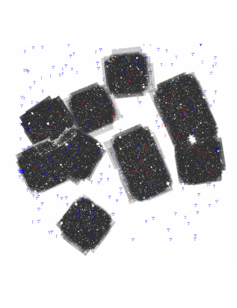
The Spitzer IRAC data were reduced using the MOPEX software (Makovoz & Khan 2005) provided by the Spitzer Science Center. The original Spitzer basic calibrated (BCD) images were drizzled onto a grid of 0.6^′′ per pixel. From the combined Cryo mission data we have four pointings; two pointings are approximately 7^′ $\times$ 7^′ in size, the other two are approximately 7^′ $\times$ 12^′ in size. The Warm mission data covers the same four pointings, plus five additional 7^′ $\times$ 7^′ pointings; giving a total coverage area of approximately 510 square arcminutes. Within the MOPEX package we used the standard routines, as well as using the background matching routine, “overlap.pl”, to match the background between pointings. Figure 1 shows a mosaic of all of the pointings in the 3.6 $\mu$ m IRAC band, including both cryo and warm mission data.

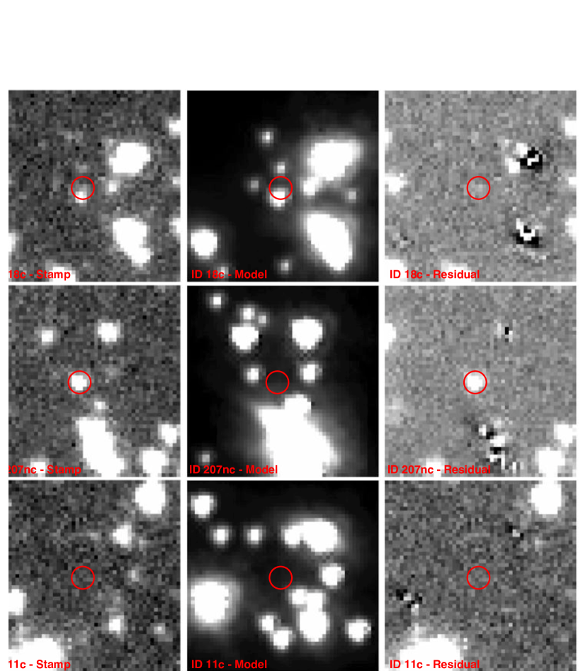
Once the IRAC data were mosaicked together, we used the galaxy fitting software GALFIT (v3.0; Peng et al. 2010) to extract mid-IR fluxes of the Spitzer-detected LAEs. Due to contamination and crowding in the IRAC images, we used GALFIT to fit and subtract nearby sources around each candidate LAE. Figure 2 shows three LAE stamps, showing a range in detectable sources and GALFIT modeling and subtraction success for nearby sources. The LAE in the bottom panel is a $z=$ 5.7 candidate LAE, and the middle and top panels are $z=$ 4.5 LAEs. The three panels for each LAE in Figure 2 show the original IRAC 3.6 $\mu$ m image, the GALFIT model, and the residual image. For the Spitzer data, we ran Source Extractor on the IRAC images prior to GALFIT to estimate input magnitudes, radial profile, and positions of other sources in the image. GALFIT was run on each of the IRAC images on a 30^′′ $\times$ 30^′′ region centered on the known LAE location, fitting all sources. GALFIT requires both an uncertainty image and a PSF. The uncertainty images from the MOPEX mosaicing of each field were used, and we constructed PSFs using stars in each IRAC mosaic. For galaxies that were detected with GALFIT, we quote the GALFIT flux and error. For galaxies without IRAC detections, aperture photometry was performed with Source Extractor (Bertin & Arnouts 1996), using a fixed aperture radius of 9 pixels or 5.4 pixels, on the residual image to obtain a flux measurement at the known source location. In fields where crowding and blending of sources is an issue that was difficult to overcome, even with the careful GALFIT modeling, or where there was a poor GALFIT subtraction of neighboring sources, we used the distribution of residual flux around the LAE to arrive at an independent flux error estimate. This was done by measuring the surrounding residual flux around the known LAE position, measured with SExtractor using fixed apertures as above, and taking an average residual flux value. When this value was comparable to the measured aperture flux from the LAE location, then it was set as the flux error, which was deemed more accurate than just taking the flux error from either GALFIT or SExtractor of the LAE itself.

For the HST WFC3 near-IR data reduction we used the multidrizzle software (2009: Koekemoer et al. 2002) to reduce and stack the data with 0.128 arcsec per pixel resolution. The raw images were processed through the CALWF3 task (v2.1: 2010) included in the IRAF STSDAS package, and the reference files were obtained from the STScI. Two of the four images were affected by noticeable persistence due to a bright target exposure prior to these two images. We corrected these two images for persistence using a persistence removal software for WFC3 IR detectors (K. Long: private communication). In order to align individual images for stacking, we used the ’tweakshift’ task to compute these shifts. Finally, the flat-fielded, persistence corrected and spatially matched images are drizzled and combined to produce a final stack. We followed a similar procedure for both F110 & F160W filters. For NICMOS data reduction, we used NICRED (Magee et al. 2007), a custom-designed pipeline to reduce NICMOS data. This pipeline corrects data for persistence, non-linear count rates, bad pixels, and pixels that are affected by cosmic rays. In addition, it performs sky-subtraction before drizzling individual images onto a final mosaic image. The high spatial resolution of the HST images allowed us to perform aperture photometry to extract the near-IR fluxes.

The deep ground-based data were reduced using standard IRAF packages, see the reduction details in Rhoads et al. 2000. To measure the ground-based optical broadband and narrowband fluxes, aperture photometry was also performed with Source Extractor, using aperture radii of 4.5 pixels, or 1.2^′′. Aperture corrections were estimated and applied, based on the difference between the $R$ -band Sextractor MagAuto magnitude and the aperture magnitude.

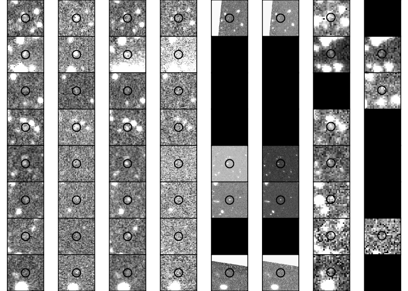
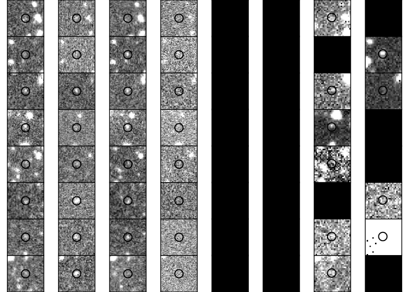
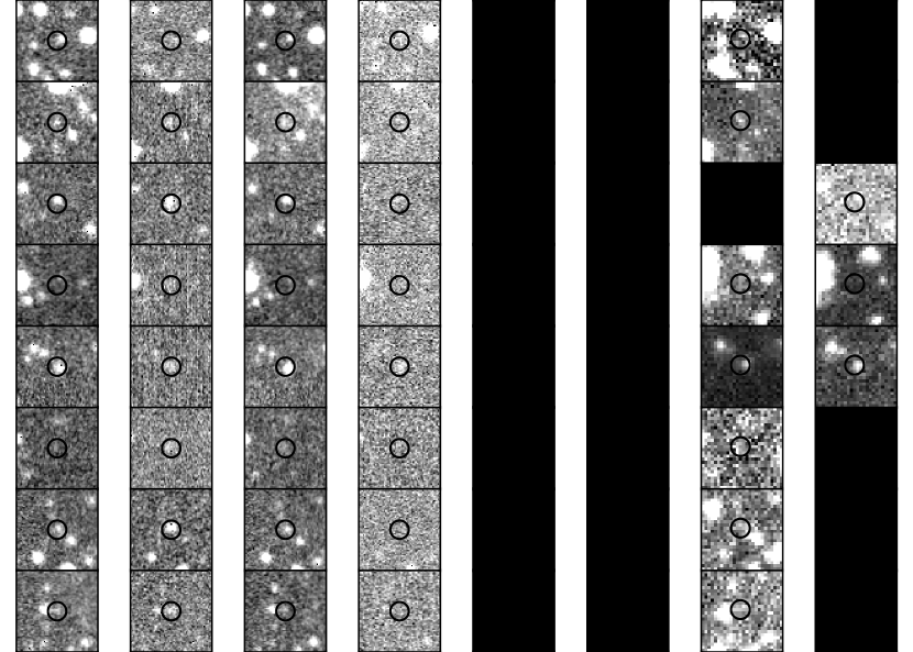
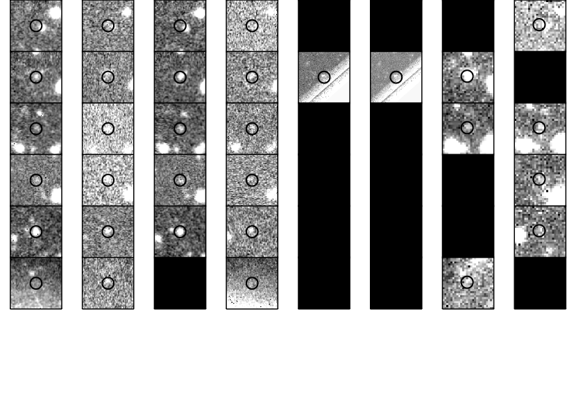
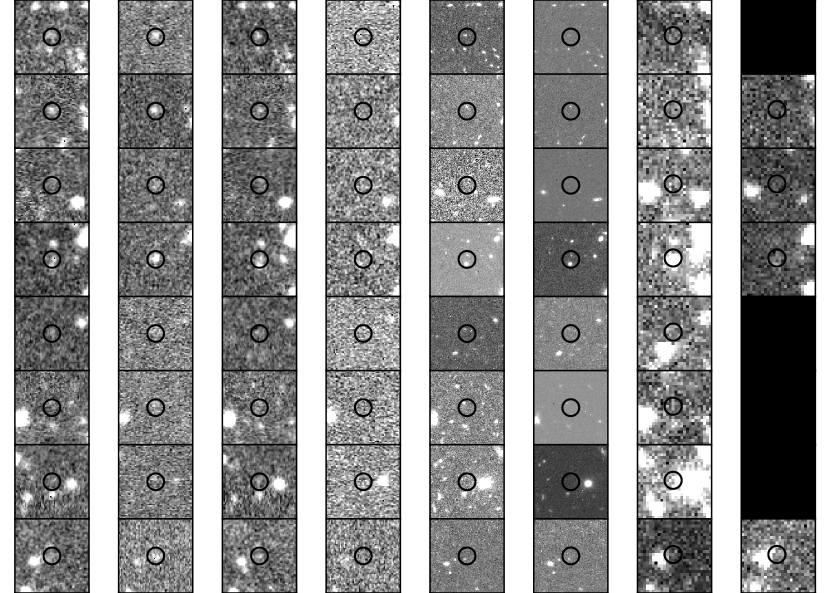
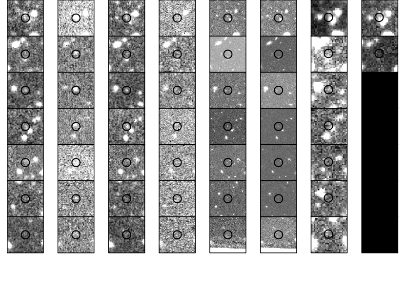
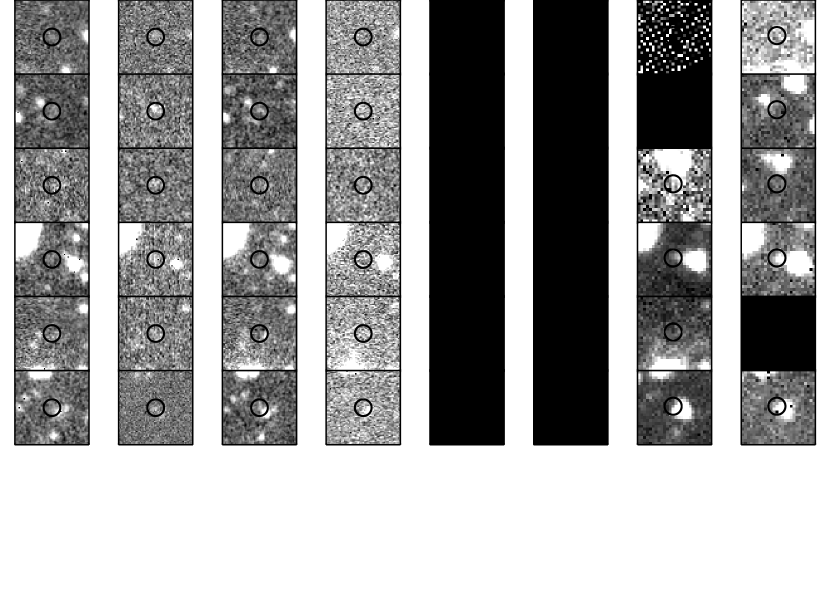
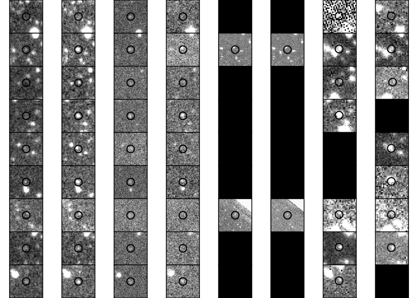
Figures 3–5 show stamps of the 30 $z=$ 4.5 candidate LAEs that are detected at $\geq$ 3 $\sigma$ in at least one IRAC band. Figure 6 shows the 15 LAEs that are only confidently detected in HST NIR bands, but have an upper limit in IRAC ( $\textless$ 3 $\sigma$ ). Figure 7 shows a selection of $z=$ 4.5 and 5.7 LAEs that are not detected in either IRAC or HST, highlighting in some cases the difficulty of extracting IRAC fluxes in crowded / blended regions, or sources where the LAE is too faint and not detected above the IRAC background. Figure 8 shows stamps of the $z=$ 5.7 LAEs, 9 of the 14 candidates with IRAC coverage were detected in at least one IRAC band. Table 1 gives a summary of the total number of sources with IRAC and/or HST NIR coverage, as well as the number of sources detected in each band at greater than 3 $\sigma$ and the resulting detection probabilities.

In order to estimate the range of best-fit stellar properties of the IRAC-undetected sample we performed a stacking analysis. We performed median flux stacking for all the filters in the IRAC un-detected sample. This method has been shown by Vargas et al. (2014) to be an improvement over median combined image stacking to estimate the fluxes in a stack. We also stacked the IRAC-detected sample in order to compare the average stellar properties between the two populations. To estimate the errors on the median-derived fluxes for each band we performed a bootstrap resampling with replacement of the individual objects in the stack. Stacking was not performed on the $z=$ 5.7 sample, because of the small number of objects in this dataset, as well as the fact that a large majority of this sample was individually detected in IRAC, therefore deeming a stacking analysis unnecessary.

3.1. Stellar Population Fitting

To determine the physical properties of the LAEs we performed spectral energy distribution (SED) fitting, using the updated (2007) version of the Bruzual & Charlot (2003) stellar population synthesis models. We used all available flux measurements from the $B$ -band to the IRAC mid-IR bands (the narrowband fluxes were not used in the fitting). The observed fluxes for each of the IRAC and/or NIR detected galaxies used in the SED fitting are listed in Table 2 for the $z=$ 4.5 sample and in Table 3 for the $z=$ 5.7 sample. IRAC flux errors are estimated from GALFIT for the sources with IRAC detections, while flux errors for the aperture-based photometry are taken from SExtractor. We also apply an additional flux error (5 $\%$ of the flux) to all measurements when doing the fitting to account for additional sources of systematic error such as uncertainties in the zeropoints for the ground-based data, and aperture correction differences.

To estimate the physical properties of each galaxy, we take our flux measurements and compare them to a grid of models, assuming a Salpeter IMF. The redshift of each source was fixed in the fitting, based on spectroscopic confirmation when available, or otherwise at the redshift that places Ly $\alpha$ in the narrowband filter with the strongest flux excess. We used empirical intergalactic medium (IGM) opacity (e.g. Madau 1995) in the models, and allowed for varying levels of dust extinction (assuming the extinction curve of Calzetti et al. 2000). Our grid parameter space contained 47 discrete values for dust, with E(B-V) between 0 – 1. The grid was more finely sampled at small E(B-V) values, and more coarsely sampled at larger values. We also account for nebular emission by using the prescription of Salmon et al. (2015). The nebular emission line strengths depend on the number of ionizing photons which is set by the stellar population age, metallicity, and ionizing escape fraction (see Salmon et al. 2015 for more details). While we do not include the narrowband fluxes as constraints in our SED fitting process, Ly $\alpha$ emission is included in our nebular spectrum, and so the contribution of the observed line to the broadband flux can be accounted for. However, we acknowledge that the radiative transfer of Ly $\alpha$ is complicated, in that the geometry and kinematics of the interstellar medium (ISM) combined with the resonant scattering properties can result in an emergent Ly $\alpha$ strength which is different than the model predictions (as our model assumes that Ly $\alpha$ experiences the same dust attenuation as continuum photons at similar wavelengths). Modeling these ISM properties is outside the scope of this analysis, but we note that those studies which have examined the escape of Ly $\alpha$ photons have found that Ly $\alpha$ does not appear to, on average, suffer any “extra” attenuation due to these effects (e.g., Finkelstein et al. 2009; Blanc et al. 2011). This is confirmed as the ratio of the observed Ly $\alpha$ flux to that of the best-fit model predicted flux has a median value close to unity (for IRAC-detected sources). However, there is a non-negligible spread, in that $\sim$ 40% of these galaxies have narrowband observed-to-model flux ratios which differ by more than a factor of two from unity. Thus, while Ly $\alpha$ does not appear to be dramatically attenuated more than continuum photons on average, this can clearly vary on a galaxy by galaxy basis.

Ages of galaxies in the models are allowed to vary from 10 Myr to the age of the universe at these redshifts; with specific grid values in steps of 1 Myr between 10 – 20 Myr; in steps of 5 Myr between 20 – 100 Myr; and in steps of 100 Myr between 100 – 1000 Myr . Metallicity is also allowed to vary with discrete values of [0.02, 0.2, 0.4, 1.0] Z_⊙. Star formation histories in the models are varied, with exponentially decaying and increasing star formation timescales. SFH = exp^-t/τ, with $\tau$ = [0.1, 1, 10, 100, 1000, 10⁴, -300, -1000, -10⁴] Myr. The shortest (0.1 Myr) and longest (10 Gyr) values of $\tau$ approximate a single burst, and continuous star formation, respectively. Model fluxes are calculated by integrating the model spectrum weighted by each filter’s transmission curve. We then find the best-fit model via $\chi^{2}$ minimization, with $\chi^{2}$ defined as:

\chi^{2}=\sum\limits_{filters}\frac{(f_{obs}-f_{mod})^{2}}{\sigma_{obs}^{2}}

(1)

We fit the SEDs of individual galaxies with IRAC detections or IRAC upper limit constraints to stellar population synthesis models. To determine the uncertainty on our best-fit stellar population properties we ran 10³ Monte Carlo simulations on each object, varying the input flux measurements by an amount drawn from a Gaussian distribution with a standard deviation equal to the flux errors for a given filter. We then determine the 68% confidence range by finding the central 68% of results for a given parameter. We list the best-fit and 68 $\%$ confidence interval results from the SED fitting for each galaxy (both the $z=$ 4.5 and $z=$ 5.7 samples) in Tables 4 –6.

4. Results

4.0.1 Stellar Mass Ranges – Results with and without Nebular Emission

To study the effects that nebular emission, especially H $\alpha$ emission in the 3.6 $\mu$ m band, has on the derived stellar mass and other properties, we fit the galaxies both with and without nebular emission.

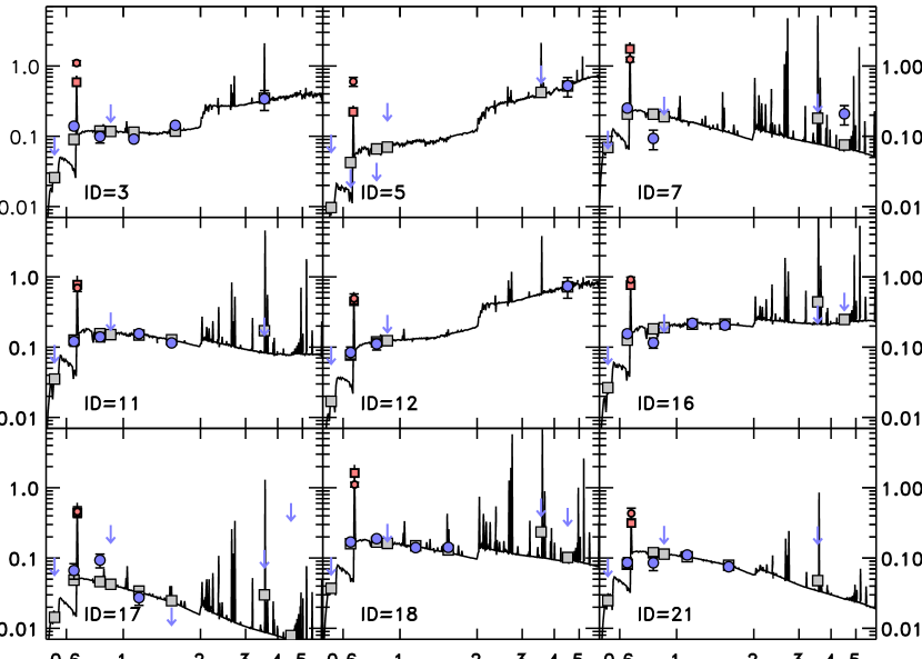
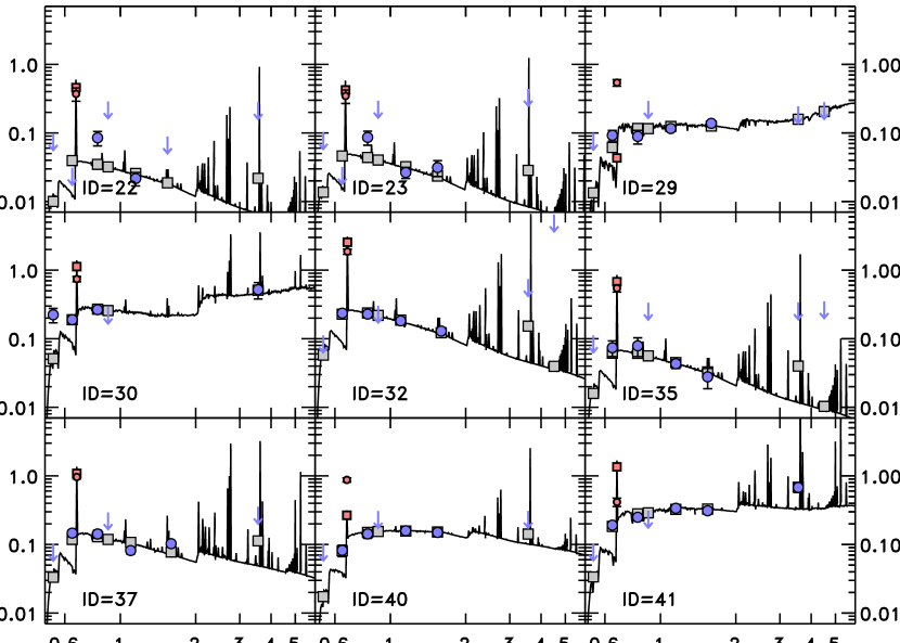
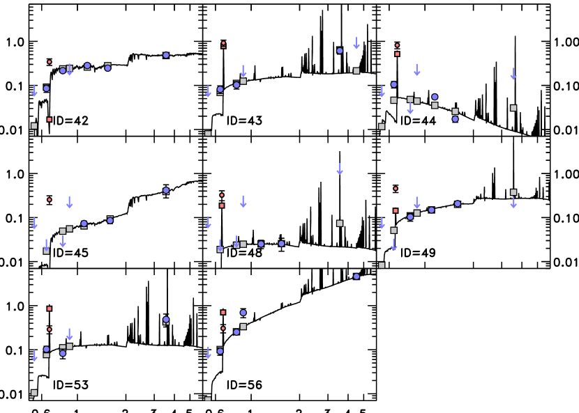
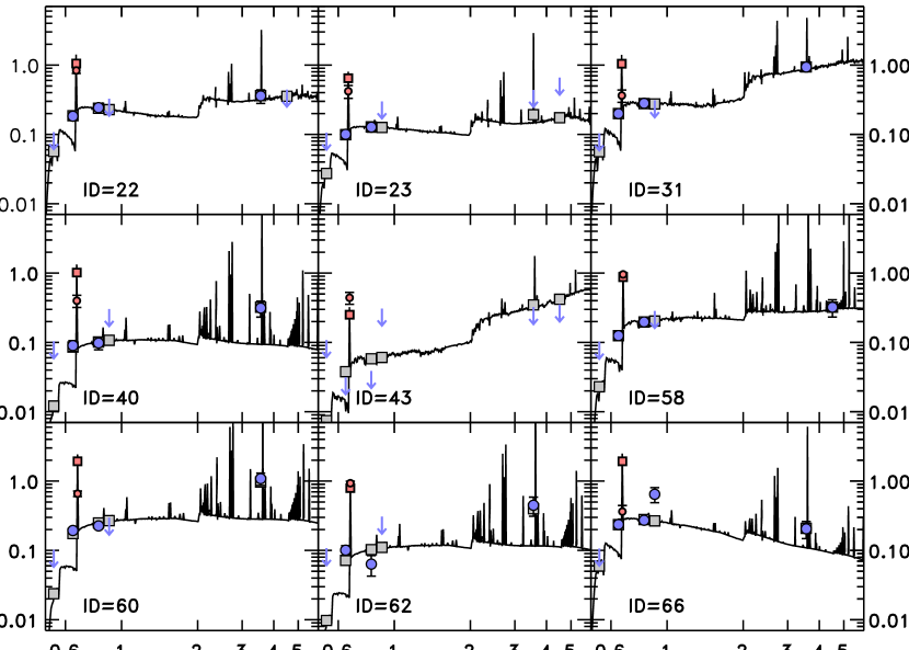
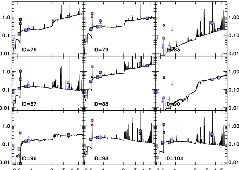
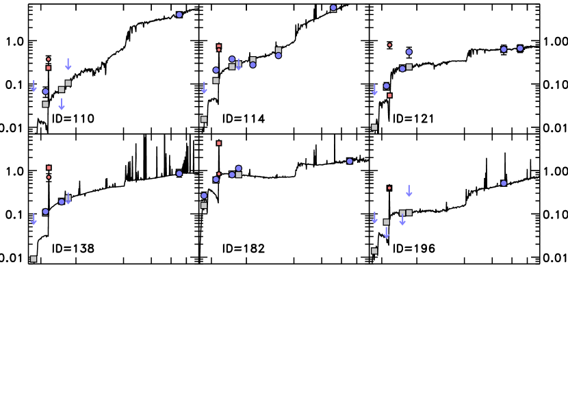
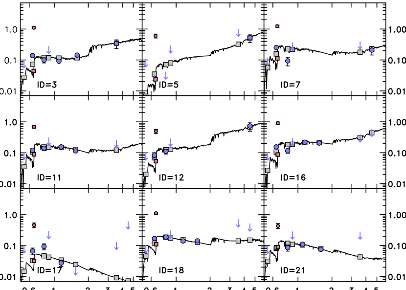
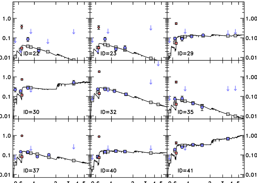
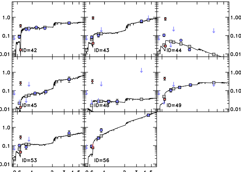
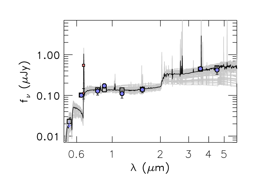
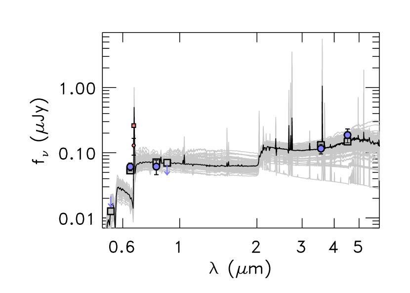
Figures 9–14 show samples of the best-fit SEDs for the HST/NIR and IRAC-detected objects, and are fit including nebular emission. We plot the 1 $\sigma$ error bars on each data point, and fluxes with less than a 3 $\sigma$ detection are shown by an upper limit. Figures 15 – 17 plot a sample of the spectroscopically confirmed objects which have detections in the IRAC bands (the same sample that is shown in Figures 8 – 10), but this time the objects have been fit without including nebular emission (all other allowable SED fitting parameters were kept the same). For the most part, especially for the IRAC-detected sample, the quality of the fits without nebular emission tend to be worse, with larger $\chi^{2}$ values derived from the best-fits. For the IRAC-detected LAEs fit with nebular emission, we find that the typical masses range from 5 $\times 10^{8}$ – few $\times$ 10¹¹ M_⊙.

The ages also show a large range, with about one-third of the IRAC-detected LAEs having stellar population ages between a few 100 Myr – 1 Gyr, and the other two-thirds with ages between 10 Myr – 100 Myr. When these same galaxies are fit without nebular emission, we find the ages are consistently higher, with a majority having best-fit ages between 600 Myr – 1 Gyr. When comparing the best-fit stellar population ages of the IRAC detected sample in the two different fitting methods, we find only 11 out of 30 LAEs (37 $\%$ ) have ages greater than 100 Myr when fitting with nebular emission, whereas 22 out of 30 (73%) have ages over 100 Myr when fitting without nebular emission. We find a mean age ratio of Age_neb / Age ${}_{no~{}neb}$ $=$ 0.5; an individual LAE is 50 $\%$ more likely to have a best-fit stellar population age greater than 600 Myr if the fit is done without including nebular emission. Nebular emission is thus a crucial ingredient when fitting this population of star-forming galaxies.

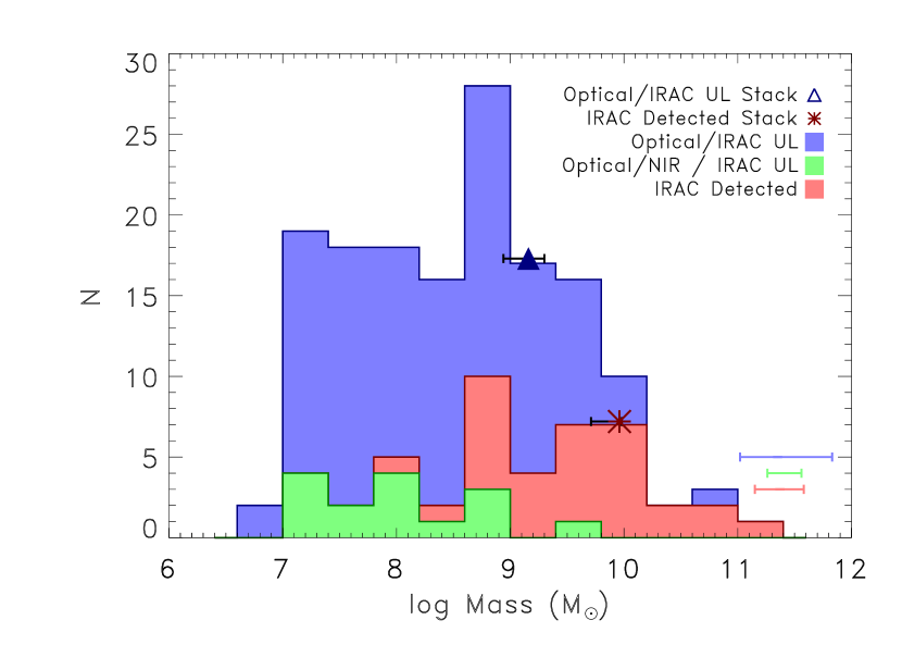
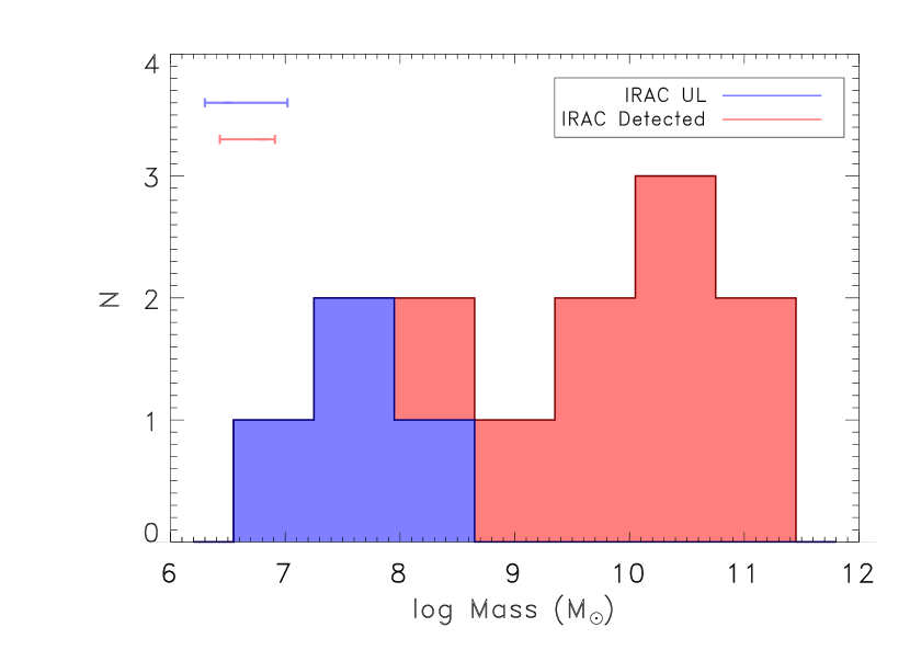
Figure 18 shows a histogram of the best-fit masses for the $z=$ 4.5 LAEs, including errors determined from the Monte Carlo simulations for the IRAC-detected, and the NIR-detected sample and optical-only detected samples with upper limits in one or more of the IRAC bands. The IRAC detected objects are typically more massive than the LAEs that are only detected in the NIR or optical by one order of magnitude. The best-fit masses for both the IRAC and NIR samples tend to have typical mass errors of $\sim$ 0.2 dex, as compared to 0.4 dex for the IRAC non-detected sample, demonstrating that the addition of the IRAC fluxes leads to more robust SED fitting results, specifically on the stellar mass estimates. While the HST-only detected sources do not have full IRAC detections, they all have IRAC upper limits, and our fits show that when we have reliable HST NIR data that is coupled with IRAC upper limits which are close to the HST detections, it becomes a reasonable constraint on the SED fits. Typically in these cases, a large 4000 Åbreak is not allowed, and we end up with a lower stellar mass sample, with reasonable constraints for the HST-only detected LAEs. When the IRAC upper limit is not close to the HST detections, then the fit is less constraining and we do have higher uncertainties on the stellar mass estimates for these LAEs. The best-fit masses for the two stacks (IRAC-detected; IRAC-undetected) are also plotted in Figure 18. By stacking the individual LAEs we saw improvement in the range of best-fit masses, especially for the IRAC-undetected stack as compared to individual LAEs in the blue histogram.

Figure 19 shows the mass histogram for the $z=$ 5.7 candidate LAEs. Nine objects are detected in IRAC and/or the NIR. These objects are some of the brightest in the IRAC sample, and appear to be relatively massive at this redshift. There are four objects at this redshift that only have measured upper limits in IRAC, and these tend to be less massive.

4.0.2 Age and Dust Results

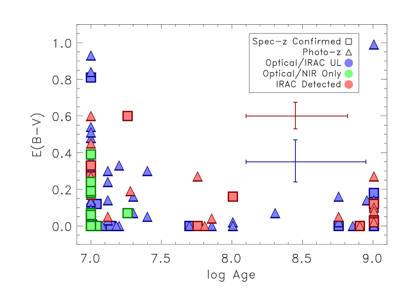
The best-fit age and E(B-V) for each galaxy are shown in Figure 20. The errors on the age distribution and dust are less constrained, and we see a spread in both age from 10 Myr – 1000 Myr, and dust from 0 – 1 magnitudes of dust reddening. LAEs with best-fit ages of 10 and 1000 Myr are falling right on the parameter endpoints in our grid, therefore we cannot say anything meaningful about the specific stellar population age in these cases, especially those that have 68% confidence in age that lies in one grid space, e.g. from 10 – 10 Myr or 1000 – 1000 Myr, and we can only conclude that these LAEs are likely very young or old.

As has been shown in Pirzkal et al. (2012), as the photometric uncertainty increases in the observations, degeneracy between stellar ages and extinction also increases. The addition of the IRAC data is expected to help break this degeneracy; however when looking at typical uncertainties in both age and dust parameters for both the IRAC-detected sample and IRAC-undetected sample, we do not see any large systematic improvement in the range in age and dust estimates. However, we do see in some of the objects (but not all) with reliable HST NIR data, that they have more robust constraints on the stellar age and dust parameters for these individual galaxies. A broad conclusion we can make, is that while $z=$ 4.5 LAEs are typically young (ages $\textless$ 100 Myr), there is a smaller population of more evolved LAEs, with ages between 500 - 1000 Myr, and this population tends to be have smaller amounts of dust. Overall, for the IRAC detected sample, we see a typical uncertainty on the stellar age of $\pm$ 0.35 dex, compared to $\pm$ 0.42 dex for the non-IRAC detected sample; similar uncertainties of $\pm$ 0.07 (IRAC detected) and 0.12 (non-IRAC detected) on E(B – V) are seen for both samples.

There is a small trend of increasing age with decreasing dust content, but again the errors on both parameters show that we cannot reliably constrain the stellar ages with the current models and observations, therefore making it difficult to make strong conclusions about this parameter. We do see that in general the smaller sample of optical and NIR detected objects only (green data points) tend to be young and with only a smaller amount of dust, from 0 – 0.4 magnitudes of dust. The more massive sample of IRAC detected LAEs (red points) tend to span a wider range in both properties, as do the optical only / IRAC upper limit detected LAEs. Overall, for both of these samples we see that the classical SED fitting is still not allowing us to break the issue of age / dust degeneracy, and therefore we cannot fully explore this issue.

4.0.3 Stacking Results

The best-fit SEDs fit to the data for the two stacked samples are shown in Figure 21. In this figure we also show the range for 100 of the best-fit SEDs from the Monte-Carlo simulations (light grey lines). By stacking the data, we again confirm that the IRAC-detected objects on average are more massive than those that are undetected in the IRAC bands. We obtain a median best-fit stellar mass of 1.5 $\times$ 10⁹ M_⊙ (0.86 – 2.0 $\times$ 10⁹ M_⊙ 68% confidence) for the IRAC-undetected stack, and best-fit mass of 9.2 $\times$ 10⁹ M_⊙ (5.1 – 9.5 $\times$ 10⁹ M_⊙ 68% confidence) for the IRAC-detected stack. This stacking analysis demonstrates that the addition of the median fluxed combined stacked IRAC data helps better constrain the range of models, as seen by the smaller spread in stellar mass for the IRAC-undetected stack as compared to the individual IRAC-undetected LAEs. The IRAC-detected stack does appear to have a slightly better constrained fit on stellar mass than the IRAC-undetected stack, shown by the smaller spread in best-fit SEDs plotted in the left-hand panel of Figure 20, as well as a somewhat smaller range on the stellar masses.

The range in other parameters, such as age and dust, do not appear to be much better constrained in the IRAC-detected stack as compared to the IRAC-undetected stack. The SED fitting results from the stacking analysis are summarized in Table 7. From the Monte-Carlo simulations, we measure a 68 $\%$ confidence range in best-fit values of E(B – V) of 0.01 – 0.17 and 0.00 – 0.09 for the IRAC-detected stack, and IRAC-undetected stack, respectively. We measure a 68 $\%$ confidence range for age of 203 – 1015 Myr and 64 – 570 Myr for the IRAC-detected stack, and IRAC-undetected stack, respectively. Stacking thus allows us to place some constraints on the age and dust attenuation, even in low-mass galaxies which were individually undetected with IRAC. However, we find here (similar to previous works, e.g. Nilsson et al. 2011; Pirzkal et al. 2012; Aquaviva et al. 2013) that even when stacking, we still obtain tighter constraints on the stellar mass than other physical properties.

5. Discussion

5.1. Stellar Masses – Comparison to other LAE studies

Other recent studies of LAEs and LBGs at similar redshift have used Spitzer IRAC observations to try to better constrain the stellar masses and other properties of z $\sim$ 4 galaxies. We compare our derived $z=$ 4.5 LAEs stellar population properties to previous studies of LAEs that have made use of IRAC observations. The Lai et al. $z=$ 3.1 sample was stacked into an IRAC-detected and IRAC-undetected sample, with the IRAC detected sample having an average mass of 9 $\times$ 10⁹ M_⊙, and the undetected sample having an average mass of 3 $\times$ 10⁸ M_⊙. This is comparable to our $z=$ 4.5 results, with the IRAC-detected stack being more massive at both redshifts, with our $z=$ 4.5 IRAC-detected stack having a best-fit stellar mass of 9 $\times$ 10⁹ M_⊙, and our IRAC-undetected stack having a best-fit stellar mass of 15 $\times$ 10⁸ M_⊙. Individually, when we compare our IRAC-detected objects to those fit by Finkelstein et al. (2008) at the same redshift, we find a similar overlap for some of our IRAC-detected sample, but with a fraction of our sample having higher masses. Of those detected in at least one IRAC band in the $z=$ 4.5 LAE sample from Finkelstein et al. (2009), they find a range of stellar masses of 3 $\times$ 10⁸ – 6 $\times$ 10⁹ M_⊙, we find LAEs in this same mass range in our sample, however we also have 11 galaxies with best-fit masses greater than 10¹⁰ M_⊙, representing 7 $\%$ of our total sample. Of our massive LAEs, 20 $\%$ come from the spectroscopically confirmed sample; this is somewhat similar to the overall sample breakdown between spec-z galaxies and non-spec-z galaxies, with 30% of the total galaxies observed with IRAC being a spec-z confirmed LAE. Detecting a higher fraction of massive LAEs as compared to Finkelstein et al. (2009) is likely due to the much larger survey area of our study, allowing for detection of a fraction of LAEs that represent the rare, most massive, more evolved population of galaxies at this redshift. However, it is possible that some of these massive galaxies which are not yet spectroscopically confirmed could be lower redshift interlopers, though the fraction is likely small, given the overall $\sim$ 75% spectroscopic confirmation success rate (Dawson et al. 2007).

5.2. H $\alpha$ Emission

In addition to better constraints on stellar mass, the Spitzer IRAC data can tell us about possible contribution to the SED from H $\alpha$ emission. There are clearly cases in our sample where there is a high 3.6 $\mu$ m band-flux, and the best-fit template fits this with a strong H $\alpha$ flux. Examples of this include sources 43c, 53c (Fig. 11); and 40nc, 60nc, 62nc (Fig. 12). In these sources, the observed narrowband photometry is also a good match to the predicted Ly $\alpha$ flux from the best-fit templates, even though the narrowband fluxes were not used in the fits. This implies that despite the uncertainties in the radiative transfer of Ly $\alpha$ , our simple assumptions regarding Ly $\alpha$ escape discussed in §3.1 may be appropriate.

In a recent study, Stark et al. (2013) derive an H $\alpha$ equivalent width distribution for their sample of 92 spectroscopically confirmed LBG galaxies at $z=$ 3.8 – 5, based on the 3.6 $\mu$ m flux. They find an average rest-frame H $\alpha$ equivalent width of 270 Å, indicating that nebular emission contributes at least 30 $\%$ to the 3.6 $\mu$ m flux. Shim et al. (2011) also have a sample of 74 z $\sim$ 4 LBGs detected in Spitzer IRAC 3.6 and 4.5 $\mu$ m observations. They show that 70 $\%$ of their sources show an excess in 3.6 $\mu$ m over the stellar continuum. In this sample of LAEs we have 22 sources with IRAC 3.6 $\mu$ m detections above 3 $\sigma$ , of those 22 sources 7 are from the spectroscopically confirmed sample, and the other 15 are from the narrowband-selected sample. Of these 22 sources, 11 have 3.6 $\mu$ m emission above the stellar continuum as determined from the best-fit SED. This corresponds to 50 $\%$ of this subset sample having H $\alpha$ emission above the stellar continuum, somewhat comparable to the 70 $\%$ in the Shim et al. sample. However, the presence of an emission line (i.e. a 3.6 $\mu$ m excess) implicitly makes a given object easier to detect with IRAC. A conservative lower limit to the fraction with strong H $\alpha$ emission would be $>$ 9% (11 with a 3.6 $\mu$ m excess compared to 123 total 3.6 $\mu$ m-observed galaxies).

We also see when only looking separately at the spectroscopically confirmed sample, and the non-spectroscopically confirmed sample, that both samples of IRAC-detected objects have similar fractions of 50 $\%$ with 3.6 $\mu$ m detections have emission above the stellar continuum. This similar fraction of an excess in 3.6 $\mu$ m over the stellar continuum in both our samples gives credence to our narrowband only selected LAEs, indicating both samples are probing similar properties of LAEs at this redshift. While a smaller sample fraction, this subsample of spectroscopically confirmed LAEs may be a robust estimate of the true LAE population as their redshift is known, and a higher fraction of them also have HST NIR detections as well, resulting in better estimates on the SED fitting (in particular, on the continuum blue-ward of H $\alpha$ ). Given the strong Ly $\alpha$ emission from our sample of LAEs, we would expect strong H $\alpha$ as well.

5.3. Star Formation Rates vs. Stellar Mass

Previous studies at lower redshift have shown that there is a sequence of star forming galaxies, with a nearly linear relationship between star formation and stellar mass, known as the “main sequence (MS) of star formation” (e.g. Noeske et al. 2007; Daddi et al. 2007; Elbaz et al. 2007) at a given redshift. These studies have shown that the tight relations exist locally and at redshifts 1 and 2, and that the slope of the trend does not seem to evolve much with redshift. The sequence normalization does vary, with lower normalizations at lower redshift, demonstrating that higher–redshift star forming galaxies are forming stars at higher rates compared to similar mass galaxies at lower redshift. More recent work has shown that these trends continue to higher redshift. Weinzirl et al. 2011 showed that a sample of more massive galaxies at redshift 2 – 3 continues to follow the Daddi $z=$ 2 trend. Hathi et al. 2013 looked at a sample of LBGs at $z=$ 1 – 3 and a comparison sample at $z=$ 4 – 5, with both samples showing a higher normalization above the Daddi $z=$ 2 MS, though both samples are best-fit by a trend line with a logarithmic slope of 0.9, similar to z $\sim$ 2 samples from both Daddi et al. (2007) and Sawicki (2012). Even more recently, Speagle et al. (2014) have investigated the MS out to $z\sim$ 6 and find that the width of the MS distribution remains constant over time, with a spread of $\sim$ 0.2 dex. They also note that the scatter around the MS at a fixed mass may be due to scatter in time, i.e., an uncertainty in the age of the universe at a given mass and star formation rate.

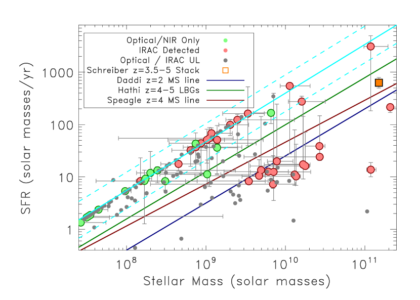
We investigate our sample of $z=$ 4.5 LAEs by placing them on the star formation rate (SFR) versus stellar mass plane. We calculated the SFR assuming the Kennicutt (1998) UV star formation calibration defined from the dust-corrected UV absolute magnitude from 1500 – 2800 Å, assuming a Salpeter IMF (as in Kennicutt 1998). Using the best-fit model for each galaxy, we calculated the model UV flux from 1500 – 2800 Å, and then corrected for dust attenuation by taking the best-fit E(B-V) dust estimate and converting it to a dust extinction at A₂₁₅₀ (assuming a Calzetti dust law). The 68 $\%$ confidence range on the dust parameters was used in determining uncertainties on the derived SFRs. The best-fit mass and derived SFR are plotted in Figure 22, with error bars based on the Monte Carlo simulations for each quantity.

We find that our sample of z $\sim$ 4.5 LAEs follow a similar linear correlation, though the normalization is higher than the z $\sim$ 2 derived MS of star forming galaxies from Daddi et al. (2007), who also assume a Salpeter IMF. Interestingly, we do find that the majority of our massive (log M/M_⊙ $>$ 9.5) LAEs fall directly on the $z\sim$ 2 trend. Fitting to the IRAC-detected and HST-detected LAEs between the mass range of 10⁷ – 3 $\times$ 10⁹, we derive a best-fit line with a logarithmic slope of 0.9 $\pm$ 0.05. In Figure 22, the solid cyan line shows this best-fit trend for our sample, extrapolated out to higher masses. The dashed cyan lines show the scatter from the best-fit line, which is $\sim$ 0.3 dex for the LAEs at $z=$ 4.5. This is similar to the spread measured by Daddi et al. of $\sim$ 0.3 dex at $z=$ 2, and by Hathi et al. of $\sim$ 0.4 dex for LBGs at $z=$ 4 – 5, although higher than the overall spread measured by Speagle et al. across multiple epochs.

For comparison, we plot the Daddi et al. $z=$ 2 (blue line), the Hathi et al. (green line) and the Speagle et al. (red line) trends at $z=$ 4 MS relations alongside our data in Figure 22. At similar redshift, our best-fit is elevated above the trend found by Hathi et al. for continuum selected galaxies, but is consistent within 2 $\sigma$ . Our results are also somewhat consistent with those of Bouwens et al. (2012), who found an average Mass–SFR relation for a sample of $z=$ 4 dropout galaxies with a logarithmic slope of 0.73 $\pm$ 0.32, and with a normalization similar to that of the Hathi et al. However, our sequence is elevated even more above the $z=$ 4 trend determined by Speagle et al. (2014) by a factor of 4–5. A recent study by Schreiber et al. (2014) using Herschel observations and stacking a sample of massive galaxies at $z=$ 3.5–5, with an average stellar mass of 2 $\times$ 10¹¹ M_⊙, finds an average SFR of $\sim$ 630 M_⊙ yr^-1 for that stack. This sample is at the upper mass end of our sample of LAEs, and appears to fall in between our two LAE populations on the SFR – stellar mass plot (orange square in Figure 21), but is consistent with the Hathi et al. LBG sample at these redshifts. However, another recent study of the SFR – stellar mass relation by Salmon et al. (2015), looking at galaxy samples at redshifts 4 – 6, found for their $z=$ 4 sample, a logarithmic slope of 0.7 $\pm$ 0.21, but with a lower normalization than what we see for our main $z=$ 4.5 LAE sample. The Salmon et al. sample has a normalization more consistent with the Daddi et al. results. Our $z=$ 4.5 LAE sample used to estimate the Mass–SFR relation is $\sim$ 3.5 $\sigma$ from the Daddi et al. $z=$ 2 MS. Overall, we find that for LAEs with stellar masses $<$ 3 $\times$ 10⁹ M_⊙, the SFR-stellar mass relation of LAEs at $z=$ 4.5 is similar in slope and spread but is elevated in normalization by 4–5 times compared to continuum-selected galaxies at the same redshift. Other recent studies of LAEs at redshifts 2 – 3 have also found that the general LAE population lies above the normal z $\sim$ 2 star forming galaxy main sequence (Song et al. 2014; Vargas et al. 2014).

To better investigate the two different populations of $z=$ 4.5 LAEs seen on the SFR versus stellar mass plot, we looked at individual stellar properties of IRAC-detected objects that have similar masses, but substantially different star formation rates. One set contains objects with SFRs above 100 M_⊙ yr^-1 and masses between a few $\times$ 10⁹ – few $\times$ 10¹⁰. There are 6 IRAC-detected objects in this set. The second set contained objects with SFRs less than 50 M_⊙ yr^-1, but within the same mass range as the first set. There are 13 IRAC-detected objects in this set. We find that the lower SFR sample (those that more closely follow the $z=$ 2 MS line) is typically older than the higher SFR sample. The lower SFR sample has best-fit ages ranging from 60 Myr – 1 Gyr, with only four galaxies having ages between 60 – 100 Myr, and all others having ages between 570 – 1000 Myr; whereas the higher SFR sample has best-fit ages ranging from 10 – 60 Myr, with only one galaxy in this higher SFR sample having a best-fit age above 20 Myr. One possible explanation for this, is that we are again seeing two populations of LAEs (similar to Finkelstein et al. 2009); one subset of galaxies is relatively young with high amounts of star formation, and the other population is older with less star-formation. These two populations could represent different paths for Ly $\alpha$ photon escape. In the younger population, the galaxies are undergoing a burst of star-formation, likely driving strong outflows, which may allow the Ly $\alpha$ photons to shift out of resonance via multiple scatterings in an outflowing ISM (e.g., Verhamme et al. 2008). For the older population, these galaxies are more evolved with lower SFRs, but they have had time to create holes in the ISM, which could allow Ly $\alpha$ photons to directly escape.

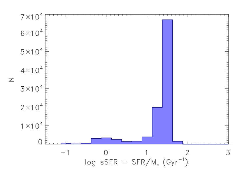
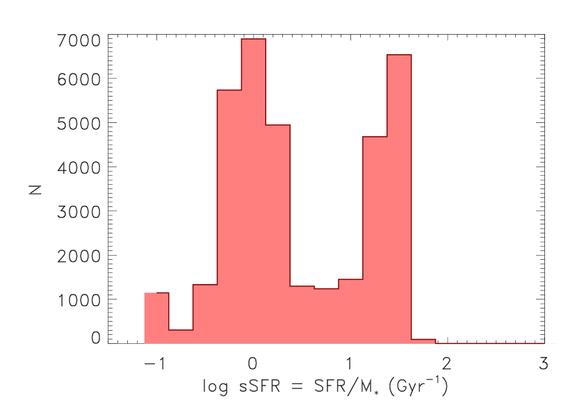
These two populations represent a bimodality in the specific SFR (sSFR) in our sample of LAEs. Out of the total sample of 150 LAEs which have IRAC constraints, we find that $\sim$ 75% have high sSFRs of 1 $\lesssim$ log (sSFR) $\lesssim$ 2, while 24% have somewhat lower values of $-$ 0.3 $\lesssim$ log(sSFR) $\lesssim$ 0.6. These latter 25% are the lower SFR, older subset of LAEs, which lie on the $z=$ 2 MS on Figure 22. However, this bimodality is seen in our best-fit values, thus to see whether it is an artifact of our SED fitting, we analyzed the full sSFR distribution using the 1000 Monte Carlo fits for each galaxy. We find that for a given galaxy in the upper or lower sequence (high or low sSFR, calculated from the best fit), the majority of the Monte Carlo simulations fall into that same sequence. This is especially true for galaxies in the upper sequence: 85 $\%$ of all 1000 Monte Carlo simulations for all galaxies in the upper sequence remain in the upper sequence. However, for the lower star-forming sequence of galaxies, typically only in $\sim$ 60 $\%$ of the simulations were they measured to have the same lower range in sSFR, while the remaining 40 $\%$ of their simulations resulted in higher calculated sSFRs. This is shown in Figure 23, where we plot the full range of measured sSFRs using the 1000 MC simulations for each source. The left-hand plot (blue histogram) shows the combined 1000 MC simulations for the 113 sources falling in the upper star forming sequence (log sSFR $\gtrsim$ 1), and the right-hand plot is the same for all 37 sources falling in the lower star forming sequence (log sSFR $\lesssim$ 0.6).

Our simulations show that for an object that has a best-fit value of the sSFR that places it in the upper sequence, it is very likely to truly have a high sSFR. However, for galaxies best-fit in the lower sequence, there is a non-negligible chance ( $\sim$ 40%) that they truly have high sSFRs, consistent with the upper sequence. This may imply that there is really only one SFR–stellar mass sequence for LAEs at $z=$ 4.5, and that our methods of measuring physical properties scatter some fraction of sources into a lower sequence. However, even if $\sim$ 40% of the sources in the low sSFR bin truly had high sSFRs, that would still leave 22 of our sample of 150 LAEs (14%) on the lower sequence (consistent with the $\sim$ 15% of LAEs from Finkelstein et al. 2009). Therefore it appears at least possible that there are two sequences of LAEs, though we are limited by the relatively small number of sources in the lower star forming sequence. In addition, as mentioned in §5.1 some of these massive galaxies have not yet been spectroscopically confirmed, and thus could be lower redshift interlopers, lowering the fraction of sources in the lower star-forming sequence, although the relatively high confirmation fraction for LAEs in general implies that a significant contamination fraction is unlikely. Further studies with larger samples may help to better address this issue of whether or not there are two populations of LAEs.

6. Summary

We have investigated a sample of 162 $z=$ 4.5 LAEs which were observed in the Spitzer IRAC 3.6 and 4.5 $\mu$ m bands. These new Spitzer observations have allowed for better constraints on the SED fitting of these galaxies, specifically for those detected with IRAC, resulting in better estimates on the stellar masses. 19 $\%$ of the $z=$ 4.5 sample were detected in at least one IRAC band, and this population of LAEs is typically more massive than the LAEs that were not detected in IRAC. When we fit the IRAC-detected galaxies individually we find typical stellar masses range 5 $\times 10^{8}$ – 10¹¹ M_⊙. The stellar ages and dust attenuation are more difficult to constrain, even with individual SED fitting and the addition of IRAC data. Only a few individual objects, typically those with additional photometry data from HST NIR , have more robust contraints on the stellar age. In general the IRAC detected objects show a wide range in best-fit values for stellar age, ranging from a 10 Myr to 1 Gyr. By analyzing the physical properties of the individual galaxies that have IRAC detections, as well as performing stacking analyses on the IRAC-detected and IRAC-undetected samples, we find the IRAC-undetected sample has an average stellar mass of $\sim$ 1.5 $\times$ 10⁹ M_⊙, and an average age of 200 Myr. Whereas, the stacked IRAC-detected sample has an average stellar mass of 9 $\times 10^{9}$ M_⊙, and an average age of 900 Myr. The stellar mass and age estimates found for this sample agree with previous studies of LAEs at this redshift, however we are also detecting a population of relatively massive LAEs at this redshift, with a handful of our IRAC-detected sample having masses between a few $\times$ 10¹⁰ – 10¹¹ M_⊙. We have also used and demonstrated the importance of including nebular emission in the stellar population fitting process. When comparing best-fit ages of individual LAEs fit with and without nebular emission lines, we find a mean age ratio of Age_neb / Age ${}_{no~{}neb}$ $=$ 0.5. This indicates that an individual LAE is 50 $\%$ more likely to have a best-fit stellar population age greater than 600 Myr if the fit is done without including nebular emission.

We have investigated the positions of our LAEs in the SFR versus stellar mass plane, and find that in general the z $\sim$ 4.5 LAE population follows a similar shape for the derived MS of galaxies at $z=$ 2, but the majority of our sample of LAEs lie above the z $\sim$ 2 MS of star forming galaxies as derived from Daddi et al. (2007), and the overall z $\sim$ 4 trend from Speagle et al. (2014). Previous studies of higher redshift galaxies (e.g. Hathi et al. 2013 & Bouwens et al. 2012) have also found that continuum–selected galaxies fall above the $z=$ 2 MS trend line, though not as high as our sample of LAEs. We conclude that at a given stellar mass, both higher redshift galaxies, and galaxies exhibiting Ly $\alpha$ in emission, produce stars at a higher rate. We do find a smaller subset of LAEs that fall below our trend line which are consistent with the $z=$ 2 MS results, indicating that there may be two mechanisms for Ly $\alpha$ escape. One where the galaxies are young, massive, and undergoing a burst of star formation,which creates large amounts of Ly $\alpha$ , and allows Ly $\alpha$ to more easily escape through an outflow in the galaxy. In the second situation, the galaxies are older, more evolved, have lower SFRs, and have had time to create holes and locations in the galaxy for the Ly $\alpha$ to escape. Although some fraction of these more evolved galaxies may truly be younger (due to degeneracies in the SED fitting process), it is possible that at least 15% of our sample of LAEs are dramatically different than the typical LAE. These possible scenarios of two methods of Ly $\alpha$ escape are directly testable by comparing the redshift of Ly $\alpha$ emission to the systemic redshift of a galaxy.

This work is based in part on observations made with the Spitzer Space Telescope, which is operated by the Jet Propulsion Laboratory, California Institute of Technology under a contract with NASA. Support for this work was provided by NASA through an award issued by JPL/Caltech. Further support for KDF and SLF was provided by the University of Texas at Austin. AD’s research activities are supported by NOAO, which is operated by the Association of Universities for Research in Astronomy under a cooperative agreement with the US National Science Foundation; and in part by the Radcliffe Institute for Advanced Study at Harvard University.

References

Acquaviva et al. (2012) Acquaviva, V., Vargos, C., Gawiser, E., & Guaita, L. 2012, ApJ, 751, 26
Bertin & Arnouts (1996) Bertin, E. & Arnouts, S. 1996, ApJS, 117, 393
Blanc et al. (2011) Blanc, G.A., Adams, J.J., Gebhardt, K., Hill, G., Drory, N., Hao, L., Bender, R., et al. 2011, ApJ, 736, 31
Bouwens et al. (2007) Bouwens, R. J., Illingworth, G. D., Franx, M., & Ford, H. 2007, ApJ, 670, 928
Bouwens et al. (2012) Bouwens, R. J., Illingworth, G. D., Oesch, P. A. et al. 2012, ApJ, 754, 83
Bruzual & Charlot (2003) Bruzual, G. & Charlot, S. 2003, MNRAS, 344, 1000
Calzetti et al. (2000) Calzetti, D., Armus, L., Bohlin, R.C., Kinney, A. L., Koornneef, J., & Storchi-Bergmann, T. 2000, ApJ, 533, 682
Cowie & Hu (1998) Cowie, L. L. & Hu, E. M. 1998, AJ, 115, 1319
Daddi et al. (2007) Daddi, E., Dickinson, M., Morrison, G., et al. 2007, ApJ, 670, 156
Dawson et al. (2004) Dawson, S., Rhoads, J. E., Malhotra, S. et al. 2004, ApJ, 617, 707
Dawson et al. (2007) Dawson, S., Rhoads, J. E., Malhotra, S. et al. 2007, ApJ, 671, 1227
Elbaz et al. (2007) Elbaz, D., Daddi, E., Le Borgne, D. et al. 2007, A&A, 468, 33
Finkelstein et al. (2011) Finkelstein, S.L., Hill, G. J., Gebhardt, K. et al. 2011, ApJ, 729, 140
Finkelstein et al. (2009) Finkelstein, S.L., Rhoads, J.E., Malhotra, S., & Grogin, N. 2009, ApJ, 691, 465
Finkelstein et al. (2008) Finkelstein, S.L., Rhoads, J.E., Malhotra, S., Grogin, N. 2008, ApJ, 678, 655
Finkelstein et al. (2007) Finkelstein, S.L., Rhoads, J.E., Malhotra, S., Pirzkal, N., Wang, J. 2007, ApJ, 660, 1023
Gawiser et al. (2006) Gawiser, E., van Dokkum, P. G., Gronwall, C. et al. 2006, ApJ, 642, 13
Gawiser et al. (2007) Gawiser, E., Francke, H., Lai, K. et al. 2007, ApJ, 671, 278
Hagen et al. (2014) Hagen, A., Ciardullo, R., Gronwall, C., Acquaviva, V., Bridge, J. et al. 2014, ApJ, 786, 59
Hathi et al. (2013) Hathi, N. P., Cohen, S. H., Ryan, R. E., Jr. et al. ApJ, 765, 88
Hu et al. (1998) Hu, E. M., Cowie, L. L., & McMahon, R. G. 1998, ApJ, 502, L99
Hu et al. (2002) Hu, E. M., Cowie, L. L., McMahon, R. G., Capak, P, Iwamuro, F., Kneib, J.-P., Maihara, T., & Motohara, K. 2002, ApJ, 568, L75
Hu et al. (2004) Hu, E. M., Cowie, L. L., Capak, P., McMahon, R. G., Hayashino, T., & Komiyama, Y. 2004, AJ, 127, 563
Kennicutt (1998) Kennicutt, R. C., Jr. 1998, ARA&A, 36, 189
Koekemoer et al. (2002) Koekemoer, A. M., et al. 2002, HST Dither Handbook, Version 2.0 (Baltimore, MD: STScI)
Lai et al. (2007) Lai, K., Huang, J.-S., Fazio, G., Cowie, L.L., Hu, E., & Kakazu, Y. 2007, ApJ, 655, 704
Lai et al. (2008) Lai, K. et al. 2008, ApJ, 674, 70
Madau (1995) Madau, P. 1995, ApJ, 441, 18
Makovoz & Khan (2005) Makovoz, D. & Khan, I. 2005, in ASP Conf. Ser. 347, Astronomical Data Analysis Software and Systems XIV, ed. P. L. Shopbel, M. C. Britton, & R. Ebert (San Fransico, CA: ASP), 81
Magee et al. (2007) Magee, D. K., Bouwens, R. J., & Illingworth, G. D. 2007, in ASP Conf. Ser. 376, Astronomical Data Analysis Software and Systems XVI, ed. R. A. Shaw, F. Hill, & D. J. Bell (San Francisco, CA: ASP), 261
Malhotra & Rhoads (2002) Malhotra, S. & Rhoads, J. E. 2002, ApJ, 565, 71
Malhotra et al. (2012) Malhotra, S., Rhoads, J. E., Finkelstein, S. L., Hathi, N., Nilsson, K., McLinden, E., & Pirzkal, N. 2012, ApJ, 750, L36
Nilsson et al. (2007) Nilsson, K. K., Mo $\o$ ller, P., M $\"{o}$ ller, O. et al. 2007, A&A, 471, 71
Nilsson et al. (2011) Nilsson, K. K., $\"{O}$ stlin, G., M $\o$ ller, P., M $\"{o}$ ller-Nilsson, O., et al. 2011, A&A, 529, A9
Noeske et al. (2007) Noeske, K. G., Weiner, B. J., Faber, S. M. et al. 2007, ApJ, 660, 43
Oke & Gunn (1983) Oke, J. B. & Gunn, J. E. 1983, ApJ, 266, 713
Ouchi et al. (2001) Ouchi, M., Shimasaku, K., Okamura, S., Doi, M., Furusawa, H., Hamabe, M., Kimura, M., et al. 2001, ApJ, 558, L83
Ouchi et al. (2003) Ouchi, M., Shimasaku, K., Furusawa, H., Miyazaki, M., Doi, M., Hamabe, M., Hayashino, T., et al. 2003, ApJ, 582, 60
Partridge & Peebles (1967) Partridge, R. B. & Peebles, P. J. E. 1967, ApJ, 147, 868
Peng et al. (2010) Peng, C. Y., Ho, L. C., Impey, C. D., & Rix, H.-W. 2010, ApJ, 139, 2097
Pentericci et al. (2000) Pentericci, L., Kurk, J., D., R $\"{o}$ ttgering, H. J. A., Miley, G. K., van Breugel, W., Carilli, C., et al. 2000 A&A, 361, 25
Pentericci et al. (2009) Pentericci, L., Grazian, A., Fontana, A., Castellano, M., Giallongo, E., Salimbeni, S., & Santini, P. 2009, A&A, 471, 433
Pirzkal et al. (2007) Pirzkal, N., Malhotra, S., Rhoads, J. E., & Xu, C. 2007, ApJ, 667, 49
Pirzkal et al. (2012) Pirzkal, N., Rothberg, B., Nilsson, K. K. et al. 2012, ApJ, 748, 122
Reddy et al. (2008) Reddy, N. A., Steidel, C. C., Petini, M., Adelberger, K. L., Shapley, A. E., Erb, D. K., & Dickinson, M. 2008, ApJS, 175, 48
Rhoads et al. (2000) Rhoads, J. E., Malhotra, S., Dey, A., Stern, D., Spinrad, H., & Jannuzi, B. T. 2000, ApJ, 545, L85
Rhoads et al. (2004) Rhoads, J. E., Xu, C., Dawson, S., Dey, A., Malhotra, S., Wang, J. X., Jannuzi, B. T., Spinrad, H., Stern, D. 2004, ApJ, 611, 59
Rhoads & Malhotra (2001) Rhoads, J. E., & Malhotra, S. 2001, ApJ, 563, L5
Salmon et al. (2015) Salmon, B., Papovich, C., Finkelstein, S. L., Tilvi, V., Finlator, K., Behroozi, P, Dahlen, T. et al. 2015, ApJ, 799, 193
Sawicki (2012) Sawicki, M. 2012, MNRAS, 421, 2187
Schreiber et al. (2014) Schreiber, C., Pannella, M., Elbaz, D., et al. 2014, A&A submitted, astro-ph arXiv: 1409.5433
Shim et al. (2011) Shim, H., Chary, R.-R., Dickinson, M., Lin, L., Spinrad, H., Stern, D., & Yan, C.-H. 2011, ApJ, 738, 69
Song et al. (2014) Song, M., Finkelstein, S. L., Gebhardt, K. et al. 2014, ApJ, 791, 3
Stark et al. (2013) Stark, D. P., Schenker, M. A., Ellis, R., Robertson, B., McLure, R., & Dunlop, J. 2013, ApJ, 763, 129
Vargas et al. (2014) Vargas, C. J., Bish, H., Acquaviva, V. et al. 2014, ApJ, 783, 26
Verhamme et al. (2008) Verhamme, A., Schaerer, D. Atek, H., & Tapken, C. 2008, A&A, 491, 89
Wang et al. (2009) Wang J.-X., Malhotra, S., Rhoads, J. E., Zhang, H.-T., & Finkelstein, S. L. 2009, ApJ, 706, 762

Table 2LAE z

\sim

4.5 Sample – Flux Measurements

ID	RA (J2000)	Dec (J2000)	NB	R	I	z’	F110W	F160W	IRAC 3.6	IRAC 4.5
3c	216.61862	35.635761	1.101 $\pm$ 0.087	0.139 $\pm$ 0.016	0.099 $\pm$ 0.019	0.115 $\pm$ 0.142	0.091 $\pm$ 0.008	0.143 $\pm$ 0.011	0.340 $\pm$ 0.108	–
5c	216.49904	35.586872	0.600 $\pm$ 0.087	0.049 $\pm$ 0.017	0.059 $\pm$ 0.021	-0.080 $\pm$ 0.148	–	–	-0.018 $\pm$ 0.508	0.524 $\pm$ 0.161
7c	216.48054	35.510797	1.237 $\pm$ 0.103	0.252 $\pm$ 0.021	0.093 $\pm$ 0.029	0.040 $\pm$ 0.182	–	–	0.580 $\pm$ 0.200	0.209 $\pm$ 0.064
8c	216.42367	35.564161	0.758 $\pm$ 0.091	0.106 $\pm$ 0.016	0.088 $\pm$ 0.020	0.117 $\pm$ 0.141	–	–	–	0.413 $\pm$ 0.163
10c	216.21837	35.436978	0.431 $\pm$ 0.073	0.049 $\pm$ 0.016	0.039 $\pm$ 0.018	0.129 $\pm$ 0.152	–	–	0.270 $\pm$ 0.123	–
11c	216.48675	35.703958	0.696 $\pm$ 0.079	0.121 $\pm$ 0.018	0.140 $\pm$ 0.021	0.149 $\pm$ 0.156	0.156 $\pm$ 0.006	0.115 $\pm$ 0.008	0.192 $\pm$ 0.132	–
12c	216.41458	35.650358	0.492 $\pm$ 0.079	0.084 $\pm$ 0.016	0.111 $\pm$ 0.020	0.135 $\pm$ 0.143	–	–	–	0.737 $\pm$ 0.240
16c	216.30292	35.631914	0.913 $\pm$ 0.080	0.155 $\pm$ 0.017	0.116 $\pm$ 0.019	0.076 $\pm$ 0.147	0.219 $\pm$ 0.006	0.205 $\pm$ 0.009	0.28 $\pm$ 0.196	0.263 $\pm$ 0.298
17c	216.29983	35.653361	0.457 $\pm$ 0.080	0.067 $\pm$ 0.017	0.093 $\pm$ 0.021	0.216 $\pm$ 0.147	0.027 $\pm$ 0.006	0.010 $\pm$ 0.010	0.174 $\pm$ 0.065	0.166 $\pm$ 0.301
18c	216.27658	35.638619	1.110 $\pm$ 0.086	0.169 $\pm$ 0.017	0.188 $\pm$ 0.020	0.136 $\pm$ 0.153	0.141 $\pm$ 0.006	0.142 $\pm$ 0.009	0.452 $\pm$ 0.352	0.258 $\pm$ 0.257
21c	216.42721	35.440425	0.431 $\pm$ 0.080	0.086 $\pm$ 0.015	0.086 $\pm$ 0.019	0.198 $\pm$ 0.143	0.111 $\pm$ 0.007	0.075 $\pm$ 0.008	-0.448 $\pm$ 0.141	–
22c	216.38225	35.447653	0.3716 $\pm$ 0.082	0.037 $\pm$ 0.015	0.085 $\pm$ 0.020	-0.043 $\pm$ 0.144	0.022 $\pm$ 0.005	-0.046 $\pm$ 0.044	-0.260 $\pm$ 0.140	–
23c	216.35883	35.425083	0.346 $\pm$ 0.077	0.047 $\pm$ 0.016	0.086 $\pm$ 0.020	-0.046 $\pm$ 0.147	0.027 $\pm$ 0.005	0.031 $\pm$ 0.008	0.072 $\pm$ 0.219	–
27c	216.77608	35.539933	0.427 $\pm$ 0.0626	0.103 $\pm$ 0.017	0.044 $\pm$ 0.021	0.220 $\pm$ 0.160	–	–	0.148 $\pm$ 0.073	-0.214 $\pm$ 0.135
29c	216.72292	35.565436	0.541 $\pm$ 0.059	0.092 $\pm$ 0.016	0.089 $\pm$ 0.020	-0.047 $\pm$ 0.146	0.116 $\pm$ 0.009	0.138 $\pm$ 0.010	-0.161 $\pm$ 0.122	0.231 $\pm$ 0.141
30c	216.61433	35.621208	0.741 $\pm$ 0.064	0.189 $\pm$ 0.017	0.265 $\pm$ 0.022	0.192 $\pm$ 0.146	–	–	0.519 $\pm$ 0.140	–
32c	216.38700	35.503331	1.864 $\pm$ 0.164	0.236 $\pm$ 0.020	0.229 $\pm$ 0.024	0.204 $\pm$ 0.152	0.182 $\pm$ 0.012	0.129 $\pm$ 0.013	-0.025 $\pm$ 0.370	0.040 $\pm$ 3.22
35c	216.28437	35.664389	0.544 $\pm$ 0.066	0.074 $\pm$ 0.019	0.079 $\pm$ 0.024	-0.101 $\pm$ 0.167	0.0433 $\pm$ 0.006	0.028 $\pm$ 0.009	-0.183 $\pm$ 0.169	-0.125 $\pm$ 0.176
37c	216.25687	35.614272	0.963 $\pm$ 0.062	0.147 $\pm$ 0.016	0.142 $\pm$ 0.019	0.158 $\pm$ 0.147	0.082 $\pm$ 0.009	0.103 $\pm$ 0.011	0.313 $\pm$ 0.178	–
40c	216.20854	35.499861	0.875 $\pm$ 0.061	0.082 $\pm$ 0.016	0.143 $\pm$ 0.020	0.220 $\pm$ 0.154	0.158 $\pm$ 0.006	0.150 $\pm$ 0.008	0.112 $\pm$ 0.154	–
41c	216.18908	35.482889	0.416 $\pm$ 0.058	0.191 $\pm$ 0.017	0.249 $\pm$ 0.020	0.296 $\pm$ 0.155	0.337 $\pm$ 0.006	0.310 $\pm$ 0.009	0.678 $\pm$ 0.106	–
42c	216.18821	35.488669	0.342 $\pm$ 0.058	0.085 $\pm$ 0.016	0.216 $\pm$ 0.020	0.351 $\pm$ 0.156	0.283 $\pm$ 0.005	0.247 $\pm$ 0.007	0.487 $\pm$ 0.063	–
43c	216.45162	35.461061	0.918 $\pm$ 0.148	0.081 $\pm$ 0.016	0.102 $\pm$ 0.020	0.262 $\pm$ 0.143	–	–	0.613 $\pm$ 0.102	-0.260 $\pm$ 0.622
44c	216.44921	35.699917	0.819 $\pm$ 0.145	0.105 $\pm$ 0.018	0.033 $\pm$ 0.021	0.077 $\pm$ 0.153	0.055 $\pm$ 0.006	0.017 $\pm$ 0.003	0.289 $\pm$ 0.125	–
45c	216.43546	35.723436	0.254 $\pm$ 0.057	0.012 $\pm$ 0.016	0.036 $\pm$ 0.020	0.204 $\pm$ 0.150	0.073 $\pm$ 0.010	0.086 $\pm$ 0.013	0.417 $\pm$ 0.138	–
46c	216.15983	35.394056	0.559 $\pm$ 0.063	0.101 $\pm$ 0.017	0.172 $\pm$ 0.022	0.503 $\pm$ 0.169	–	–	–	0.545 $\pm$ 0.211
48c	216.48629	35.709244	0.323 $\pm$ 0.082	0.019 $\pm$ 0.016	0.027 $\pm$ 0.019	-0.068 $\pm$ 0.156	0.025 $\pm$ 0.005	0.026 $\pm$ 0.008	0.028 $\pm$ 0.863	–
49c	216.42500	35.432442	0.457 $\pm$ 0.087	0.021 $\pm$ 0.016	0.103 $\pm$ 0.020	-0.182 $\pm$ 0.148	0.149 $\pm$ 0.012	0.207 $\pm$ 0.013	-0.182 $\pm$ 0.151	–
53c	216.78825	35.402408	0.289 $\pm$ 0.060	0.103 $\pm$ 0.017	0.083 $\pm$ 0.021	0.088 $\pm$ 0.152	–	–	0.487 $\pm$ 0.159	–
56c	216.47771	35.555628	0.306 $\pm$ 0.065	0.092 $\pm$ 0.018	0.251 $\pm$ 0.022	0.693 $\pm$ 0.161	–	–	–	4.607 $\pm$ 0.169
10nc	216.65613	35.289208	0.389 $\pm$ 0.073	0.045 $\pm$ 0.016	0.051 $\pm$ 0.020	0.128 $\pm$ 0.148	–	–	0.474 $\pm$ 0.164	–
22nc	216.23679	35.698278	0.835 $\pm$ 0.078	0.183 $\pm$ 0.017	0.243 $\pm$ 0.021	0.029 $\pm$ 0.164	–	–	0.359 $\pm$ 0.080	0.420 $\pm$ 0.221
23nc	216.22208	35.638567	0.420 $\pm$ 0.088	0.100 $\pm$ 0.016	0.127 $\pm$ 0.019	0.156 $\pm$ 0.150	–	–	0.072 $\pm$ 0.219	0.355 $\pm$ 0.329
26nc	216.13592	35.390422	0.422 $\pm$ 0.108	0.130 $\pm$ 0.020	0.039 $\pm$ 0.024	-0.026 $\pm$ 0.188	–	–	–	0.331 $\pm$ 0.157
31nc	216.78079	35.422856	0.363 $\pm$ 0.073	0.199 $\pm$ 0.017	0.281 $\pm$ 0.021	0.156 $\pm$ 0.155	–	–	0.936 $\pm$ 0.129	–
36nc	216.59233	35.570203	0.417 $\pm$ 0.073	0.059 $\pm$ 0.016	0.093 $\pm$ 0.020	0.008 $\pm$ 0.143	–	–	0.369 $\pm$ 0.138	–
40nc	216.41279	35.755600	0.399 $\pm$ 0.079	0.090 $\pm$ 0.016	0.098 $\pm$ 0.020	0.076 $\pm$ 0.151	–	–	0.313 $\pm$ 0.081	–
43nc	216.31254	35.675472	0.441 $\pm$ 0.086	0.040 $\pm$ 0.016	0.053 $\pm$ 0.019	0.752 $\pm$ 0.615	–	–	0.256 $\pm$ 0.161	0.537 $\pm$ 0.190
44nc	216.28917	35.749864	0.340 $\pm$ 0.076	0.072 $\pm$ 0.017	0.152 $\pm$ 0.021	0.216 $\pm$ 0.154	–	–	–	0.380 $\pm$ 0.146
57nc	216.66546	35.505661	0.439 $\pm$ 0.082	0.036 $\pm$ 0.017	0.041 $\pm$ 0.022	-0.104 $\pm$ 0.153	–	–	0.180 $\pm$ 0.189	0.359 $\pm$ 0.174
58nc	216.65525	35.736069	0.957 $\pm$ 0.062	0.125 $\pm$ 0.017	0.197 $\pm$ 0.020	0.188 $\pm$ 0.142	–	–	–	0.322 $\pm$ 0.090
60nc	216.61350	35.350981	0.658 $\pm$ 0.060	0.194 $\pm$ 0.016	0.226 $\pm$ 0.019	0.245 $\pm$ 0.148	–	–	1.085 $\pm$ 0.220	–
62nc	216.58488	35.256228	0.932 $\pm$ 0.064	0.101 $\pm$ 0.016	0.063 $\pm$ 0.021	0.172 $\pm$ 0.153	–	–	0.448 $\pm$ 0.138	–
66nc	216.46129	35.762097	0.364 $\pm$ 0.081	0.236 $\pm$ 0.018	0.272 $\pm$ 0.021	0.645 $\pm$ 0.158	–	–	0.205 $\pm$ 0.057	–
76nc	216.82129	35.441064	0.445 $\pm$ 0.064	0.120 $\pm$ 0.020	0.187 $\pm$ 0.025	0.117 $\pm$ 0.159	–	–	1.085 $\pm$ 0.110	–
79nc	216.78329	35.353919	1.056 $\pm$ 0.064	0.228 $\pm$ 0.016	0.279 $\pm$ 0.021	0.618 $\pm$ 0.162	–	–	–	0.870 $\pm$ 0.152
83nc	216.67629	35.493894	0.342 $\pm$ 0.061	0.017 $\pm$ 0.016	-0.009 $\pm$ 0.021	0.082 $\pm$ 0.146	–	–	0.461 $\pm$ 0.146	-0.165 $\pm$ 0.155
87nc	216.64671	35.252078	0.385 $\pm$ 0.062	0.111 $\pm$ 0.016	0.149 $\pm$ 0.021	0.255 $\pm$ 0.147	–	–	0.249 $\pm$ 0.086	–
88nc	216.64079	35.450736	0.507 $\pm$ 0.060	0.285 $\pm$ 0.017	0.461 $\pm$ 0.021	0.890 $\pm$ 0.146	–	–	2.603 $\pm$ 0.072	2.125 $\pm$ 0.117
90nc	216.63858	35.439358	0.455 $\pm$ 0.062	0.032 $\pm$ 0.017	-0.010 $\pm$ 0.021	0.061 $\pm$ 0.154	–	–	0.323 $\pm$ 0.301	0.395 $\pm$ 0.294
96nc	216.58721	35.580183	0.407 $\pm$ 0.060	0.043 $\pm$ 0.016	0.145 $\pm$ 0.019	0.266 $\pm$ 0.142	–	–	0.302 $\pm$ 0.0840	–
98nc	216.57875	35.287997	1.067 $\pm$ 0.065	0.185 $\pm$ 0.017	0.226 $\pm$ 0.020	-0.257 $\pm$ 0.153	–	–	0.491 $\pm$ 0.160	–
104nc	216.43054	35.709911	0.444 $\pm$ 0.058	0.123 $\pm$ 0.016	0.119 $\pm$ 0.020	0.125 $\pm$ 0.148	–	–	0.340 $\pm$ 0.085	–
110nc	216.27879	35.817781	0.372 $\pm$ 0.074	0.067 $\pm$ 0.018	0.048 $\pm$ 0.023	-0.081 $\pm$ 0.194	–	–	–	3.976 $\pm$ 0.255
111nc	216.27292	35.772394	0.336 $\pm$ 0.059	0.018 $\pm$ 0.014	-0.029 $\pm$ 0.018	-0.050 $\pm$ 0.149	–	–	–	0.387 $\pm$ 0.145
114nc	216.24808	35.606881	0.615 $\pm$ 0.062	0.209 $\pm$ 0.017	0.376 $\pm$ 0.019	1.006 $\pm$ 0.149	0.275 $\pm$ 0.020	0.453 $\pm$ 0.025	5.800 $\pm$ 0.159	–
121nc	216.77842	35.574064	0.795 $\pm$ 0.148	0.090 $\pm$ 0.018	0.224 $\pm$ 0.021	0.551 $\pm$ 0.155	–	–	0.630 $\pm$ 0.157	0.666 $\pm$ 0.135
138nc	216.20413	35.333586	0.702 $\pm$ 0.149	0.113 $\pm$ 0.017	0.190 $\pm$ 0.022	0.402 $\pm$ 0.154	–	–	–	0.854 $\pm$ 0.149
182nc	216.66083	35.775336	0.840 $\pm$ 0.061	0.625 $\pm$ 0.018	0.801 $\pm$ 0.022	1.124 $\pm$ 0.151	–	–	–	1.642 $\pm$ 0.242
191nc	216.75946	35.425897	0.616 $\pm$ 0.084	0.077 $\pm$ 0.016	0.064 $\pm$ 0.020	0.264 $\pm$ 0.156	–	–	0.575 $\pm$ 0.260	–
196nc	216.21612	35.553250	0.396 $\pm$ 0.060	0.064 $\pm$ 0.025	0.102 $\pm$ 0.050	0.150 $\pm$ 0.231	–	–	0.510 $\pm$ 0.061	–

Note. — Source IDs ending in ’c’ are LAEs that have been spectroscopically confirmed. Source IDs ending in ’nc’ have a photometric redshift based on narrow-band imaging, and have not been targeted spectroscopically. RA, Dec in degrees. Fluxes are all given in $\mu$ Jy. No coverage in a Spitzer or HST band is denoted by – .

Table 3LAE z

\sim

5.7 Sample – Flux Measurements

ID	RA (J2000)	Dec (J2000)	NB	R	I	z’	F110W	F160W	IRAC 3.6	IRAC 4.5
54c	216.69638	35.603511	1.278 $\pm$ 0.122	-0.026 $\pm$ 0.019	0.081 $\pm$ 0.023	0.499 $\pm$ 0.151	–	–	-1.056 $\pm$ 0.281	–
55c	216.62629	35.672933	0.784 $\pm$ 0.119	-0.003 $\pm$ 0.018	0.044 $\pm$ 0.022	-0.060 $\pm$ 0.155	–	–	1.136 $\pm$ 0.273	0.134 $\pm$ 2.107
57c	216.39138	35.506383	1.170 $\pm$ 0.136	0.057 $\pm$ 0.028	0.662 $\pm$ 0.062	1.438 $\pm$ 0.185	2.134 $\pm$ 0.012	3.026 $\pm$ 0.014	3.277 $\pm$ 0.210	1.817 $\pm$ 0.233
58c	216.38038	35.427475	0.715 $\pm$ 0.115	0.025 $\pm$ 0.017	0.023 $\pm$ 0.020	0.024 $\pm$ 0.1465	0.006 $\pm$ 0.005	0.011 $\pm$ 0.008	-0.533 $\pm$ 0.139	–
63c	216.40554	35.480000	0.631 $\pm$ 0.102	-0.035 $\pm$ 0.016	0.052 $\pm$ 0.021	-0.194 $\pm$ 0.144	–	–	-0.375 $\pm$ 0.140	0.121 $\pm$ 0.209
202nc	216.73854	35.615664	0.563 $\pm$ 0.109	-0.006 $\pm$ 0.016	0.177 $\pm$ 0.021	0.408 $\pm$ 0.148	–	–	0.886 $\pm$ 0.22	1.379 $\pm$ 0.371
203nc	216.63029	35.496514	0.793 $\pm$ 0.111	-0.008 $\pm$ 0.015	0.049 $\pm$ 0.020	-0.077 $\pm$ 0.145	–	–	-0.037 $\pm$ 0.134	-0.116 $\pm$ 0.188
207nc	216.55396	35.640358	1.247 $\pm$ 0.116	0.061 $\pm$ 0.016	0.565 $\pm$ 0.021	1.774 $\pm$ 0.150	–	–	4.523 $\pm$ 0.124	–
209nc	216.40683	35.637464	0.799 $\pm$ 0.114	0.123 $\pm$ 0.017	0.316 $\pm$ 0.022	0.517 $\pm$ 0.148	–	–	–	11.573 $\pm$ 1.062
210nc	216.36638	35.727917	1.117 $\pm$ 0.117	0.140 $\pm$ 0.016	0.443 $\pm$ 0.020	1.133 $\pm$ 0.148	–	–	–	17.356 $\pm$ 0.477
222nc	216.72350	35.419058	0.680 $\pm$ 0.097	0.045 $\pm$ 0.016	0.129 $\pm$ 0.021	-0.014 $\pm$ 0.154	–	–	23.092 $\pm$ 2.118	23.521 $\pm$ 1.509
223nc	216.72079	35.572011	0.565 $\pm$ 0.091	-0.003 $\pm$ 0.015	0.024 $\pm$ 0.020	0.152 $\pm$ 0.148	0.184 $\pm$ 0.012	0.180 $\pm$ 0.015	0.334 $\pm$ 0.068	0.380 $\pm$ 0.095
224nc	216.63808	35.313544	0.542 $\pm$ 0.096	0.172 $\pm$ 0.017	0.216 $\pm$ 0.020	0.328 $\pm$ 0.149	–	–	2.726 $\pm$ 0.125	3.369 $\pm$ 0.309
231nc	216.46479	35.731386	0.796 $\pm$ 0.097	0.146 $\pm$ 0.017	0.343 $\pm$ 0.021	0.519 $\pm$ 0.153	–	–	0.474 $\pm$ 0.109	–

Note. — Source IDs ending in ’c’ are LAEs that have been spectroscopically confirmed. Source IDs ending in ’nc’ have a photometric redshift based on narrow-band imaging, and have not been targeted spectroscopically. The observed narrow-band for the $z=$ 5.7 sources is at 815 or 823 nm. RA, Dec in degrees. Fluxes are all given in $\mu$ Jy. No coverage in a Spitzer or HST band is denoted by –

Table 4

z=

4.5 IRAC Detected LAEs – Model SED Fitting Results

ID	Reduced $\chi^{2}$	Mass	Mass	Age	Age	E(B-V)	E(B-V)	Z	Z
	of Best Fit	Best Fit	68 $\%$ Range	Best Fit	68 $\%$ Range	Best Fit	68 $\%$ Range	Best Fit	68 $\%$ Range
		(10⁸ M_⊙)	(10⁸ M_⊙)	(Myr)	(Myr)	(mag)	(mag)	(Z_⊙)	(Z_⊙)
3c	9.6	70	2.0 – 5.9	1015	10 – 10	0.03	0.05 – 0.19	0.02	0.02 – 0.02
7c	30.2	1.5	1.4 – 7.7	10	10 – 10	0.00	0.00 – 0.13	0.20	0.02 – 0.20
12c	0.5	168	54 – 204	1015	10 – 1015	0.12	0.04 – 0.39	0.02	0.02 – 0.20
30c	10.4	61	17 – 109	806	45 – 1015	0.00	0.00 – 0.02	0.20	0.02 – 0.40
41c	3.1	12	11 – 21	10	10 – 20	0.18	0.15 – 0.21	1.00	1.00 – 1.00
42c	4.9	49	47 – 74	57	10 – 72	0.00	0.00 – 0.30	1.00	0.02 – 1.00
43c	2.3	20	15 – 35	10	10 – 12	0.33	0.27 – 0.36	0.02	0.02 – 0.02
45c	1.9	71	36 – 208	102	10 – 570	0.16	0.00 – 0.60	0.20	0.02 – 1.00
53c	4.4	11	0.8 – 22	10	10 – 10	0.27	0.00 – 0.33	0.02	0.02 – 0.02
56c	5.0	1184	973 – 1954	18	10 – 90	0.60	0.24 – 0.66	0.02	0.02 – 0.4
22nc	2.0	46.6	7.3 – 55.8	806	10 – 1015	0.00	0.00 – 0.09	0.02	0.02 – 0.40
31nc	0.9	178	36 – 200	1015	20 – 1015	0.02	0.01 – 0.21	0.20	0.02 – 0.40
40nc	0.5	74	5.2 – 28.3	10	10 – 45	0.24	0.11 – 0.27	0.20	0.02 – 0.20
58nc	0.01	13.8	12.2 – 52.5	19	10 – 905	0.19	0.00 – 0.27	0.40	0.02 – 0.40
60nc	3.3	24.9	17.8 – 130	10	10 – 1015	0.27	0.07 – 0.30	0.02	0.02 – 0.20
62nc	6.9	10.3	3.3 – 17.1	10	10 – 10	0.27	0.14 – 0.33	0.02	0.02 – 0.02
66nc	6.1	4.5	2.7 – 8.4	13	10 – 20	0.05	0.01 – 0.08	0.02	0.02 – 0.02
76nc	0.3	270	30 – 278	1015	10 – 1015	0.10	0.08 – 0.33	0.02	0.02 – 0.40
79nc	6.8	167	60.5 – 185	1015	10 – 1015	0.02	0.00 – 0.36	0.02	0.02 – 0.02
83nc	7.3	33.7	16.2 – 54.2	10	10 – 10	0.60	0.42 – 0.75	0.02	0.02 – 0.02
88nc	7.8	160	109 – 317	57	20 – 102	0.27	0.27 – 0.30	0.20	0.02 – 1.00
96nc	5.8	34.6	26 – 55.7	64	45 – 102	0.00	0.00 – 0.11	1.00	0.02 – 1.00
98nc	10.4	8.7	3.4 – 42.8	10	10 – 719	0.17	0.00 – 0.19	0.02	0.02 – 0.20
104nc	1.7	6.4	3.7 – 10.3	10	10 – 10	0.19	0.10 – 0.21	0.02	0.02 – 0.02
110nc	6.5	1187	1053 – 1381	570	570 – 570	0.05	0.01 – 0.09	1.00	1.00 – 1.00
114nc	40.6	2082	2020 – 2561	1015	1015 – 1015	0.27	0.27 – 0.30	0.20	0.20 – 0.20
121nc	8.3	77.9	59.2 – 124	72	10 – 80	0.04	0.00 – 0.36	1.00	0.02 – 1.00
138nc	1.6	113	86.0 – 205	10	10 – 1015	0.45	0.36 – 0.51	0.02	0.02 – 0.20
182nc	8.4	268	177 – 315	806	806 – 1015	0.00	0.00 – 0.00	0.02	0.02 – 0.20
196nc	0.1	130	75.4 – 116	1015	10 – 1015	0.08	0.02 – 0.33	0.40	0.02 – 1.00

Table 5

z=

4.5 HST NIR Detected LAEs with IRAC Upper Limits – Model SED Fitting Results

ID	Reduced $\chi^{2}$	Mass	Mass	Age	Age	E(B-V)	E(B-V)	Z	Z
	of Best Fit	Best Fit	68 $\%$ Range	Best Fit	68 $\%$ Range	Best Fit	68 $\%$ Range	Best Fit	68 $\%$ Range
		(10⁸ M_⊙)	(10⁸ M_⊙)	(Myr)	(Myr)	(mag)	(mag)	(Z_⊙)	(Z_⊙)
11c	2.1	2.0	2.7 – 10.3	10	10 – 20	0.06	0.04 – 0.18	1.00	0.02 – 1.00
16c	5.1	7.4	6.9 – 14.8	10	10 – 10	0.18	0.16 – 0.24	1.00	1.00 – 1.00
17c	5.2	0.33	0.3 – 16.3	10	10 – 1015	0.00	0.00 – 0.00	0.02	0.02 – 0.02
18c	1.2	2.5	2.1 – 23.5	10	10 – 905	0.07	0.00 – 0.09	0.20	0.02 – 0.20
21c	8.5	3.1	1.3 – 5.5	10	10 – 10	0.06	0.01 – 0.13	0.02	0.02 – 1.00
22c	9.4	0.3	0.2 – 0.6	11	10 – 12	0.00	0.00 – 0.00	0.02	0.02 – 0.02
23c	3.4	0.3	0.3 – 0.6	10	10 – 12	0.00	0.00 – 0.00	0.20	0.02 – 0.02
29c	5.0	10.3	2.6 – 10.4	18	10 – 18	0.07	0.01 – 0.15	1.00	0.02 – 1.00
32c	0.5	1.7	1.6 – 2.1	10	10 – 11	0.00	0.00 – 0.03	0.02	0.02 – 0.02
35c	1.5	0.4	0.4 – 0.6	10	10 – 11	0.00	0.00 – 0.00	0.02	0.02 – 0.02
37c	7.5	1.0	0.9 – 1.1	10	10 – 10	0.09	0.00 – 0.01	0.20	0.02 – 0.20
40c	0.7	13.8	5.9 – 25.1	10	10 – 40	0.19	0.04 – 0.21	0.02	0.02 – 1.00
44c	17. 0	0.4	0.3 – 0.4	10	10 – 10	0.00	0.00 – 0.00	0.02	0.02 – 0.02
48c	0.4	1.7	0.4 – 60.6	10	10 – 404	0.24	0.00 – 0.30	0.02	0.02 – 1.00
49c	7.0	65.8	39.5 – 67.0	10	10 – 10	0.39	0.33 – 0.39	0.02	0.02 – 0.02

Table 6

z=

5.7 IRAC Detected LAEs – Model SED Fitting Results

ID	Reduced $\chi^{2}$	Mass	Mass	Age	Age	E(B-V)	E(B-V)	Z	Z
	of Best Fit	Best Fit	68 $\%$ Range	Best Fit	68 $\%$ Range	Best Fit	68 $\%$ Range	Best Fit	68 $\%$ Range
		(10⁸ M_⊙)	(10⁸ M_⊙)	(Myr)	(Myr)	(mag)	(mag)	(Z_⊙)	(Z_⊙)
55c	1.1	48.8	38.3 – 505	1	1 – 404	0.45	0.00 – 0.51	0.20	0.20 – 1.00
57c	27.5	497	486 – 636	10	10 – 10	0.24	0.24 – 0.27	0.02	0.02 – 0.02
202nc	2.2	173	31.2 – 175	7	2 – 57	0.33	0.00 – 0.36	0.02	0.02 – 1.00
207nc	2.1	760	706 – 859	72	72 – 102	0.00	0.00 – 0.03	1.00	0.20 – 1.00
209nc	24.2	5150	542 – 5339	509	2 – 509	0.00	0.00 – 0.42	1.00	0.40 – 1.00
210nc	28.7	5764	5621 – 7434	509	509 – 509	0.00	0.00 – 0.06	0.40	0.02 – 1.00
223nc	1.5	53.2	42.3 – 71.6	57	50 – 81	0.00	0.00 – 0.00	1.00	0.20 – 1.00
224nc	61.4	1139	86.2 – 1332	806	3 – 806	0.15	0.03 – 0.30	0.20	0.02 – 0.20
231nc	29.0	9.95	2.89 – 35.6	7	3 – 19	0.00	0.00 – 0.00	0.20	0.02 – 0.40

Table 7

z=

4.5 LAE Stacks – Model SED Fitting Results

Stack	Reduced $\chi^{2}$	Mass	Mass	Age	Age	E(B-V)	E(B-V)
	of Best Fit	Best Fit	68 $\%$ Range	Best Fit	68 $\%$ Range	Best Fit	68 $\%$ Range
		(10⁸ M_⊙)	(10⁸ M_⊙)	(Myr)	(Myr)	(mag)	(mag)
IRAC Undetected Stack	4.8	15	8.6 – 20	203	64 – 570	0.03	0.00 – 0.09
IRAC Detected Stack	1.2	92	51 – 95	905	203 – 1015	0.06	0.01 – 0.17

Probing the Physical Properties of z=𝑧absentz= 4.5 Lyman Alpha Emitters with Spitzer