Neutrons on a surface of liquid helium

Abstract

We investigate the possibility of ultracold neutron (UCN) storage in quantum states defined by the combined potentials of the Earth’s gravity and the neutron optical repulsion by a horizontal surface of liquid helium. We analyse the stability of the lowest quantum state, which is most susceptible to perturbations due to surface excitations, against scattering by helium atoms in the vapor and by excitations of the liquid, comprised of ripplons, phonons and surfons. This is an unusual scattering problem since the kinetic energy of the neutron parallel to the surface may be much greater than the binding energies perpendicular. The total scattering time constant of these UCNs at $0.7$ K is found to exceed one hour, and rapidly increasing with decreasing temperature. Such low scattering rates should enable high-precision measurements of the scheme of discrete energy levels, thus providing improved access to short-range gravity. The system might also be useful for neutron $\beta$-decay experiments. We also sketch new experimental concepts for level population and trapping of UCNs above a flat horizontal mirror.

I Introduction

Slow neutrons play an important role in low-energy particle physics as a tool and an object, in investigations of the free neutron’s properties and its interactions with known or hypothetic fields with high precision Dubbers/2011 ; Musolf/2008 ; Abele/2008 . A particular class of experiments employs neutrons with energy lower than the neutron optical potential of typical materials, i.e. in the order of up to $300$ neV. These so-called ultracold neutrons (UCNs) can be emprisoned for many hundreds of seconds in well-designed ”neutron bottles”. By virtue of the neutron magnetic moment of $60$ neV/T magnetic trapping is feasible too, and also the gravitational interaction with a potential difference of $100$ neV per meter rise can play its role in UCN storage and manipulation Golub/1991 ; Ignatovich/1990 . Perhaps the most prominent application of UCNs is the search for a non-vanishing electric dipole moment of the neutron. Finding a finite value or just improving current limits is a way of investigating new mechanisms of CP violation beyond the standard model’s complex phase of the weak quark mixing CKM matrix, and the matter-antimatter asymmetry in the universe Pospelov/2005 . Latest experimental results were published in Refs. Baker/2006 ; Serebrov/2014 . Similarly long standing are the experimental efforts to determine the neutron lifetime with high accuracy. Its value enters the calculations of weak reaction rates in big-bang nucleo-synthesis and stellar fusion Coc/2007 ; Lopez/1999 , and it is also crucial for deriving the weak axial-vector and vector coupling constants of the nucleon needed to calculate many important semi-leptonic cross sections.

Discrete energy levels of UCNs in the Earth’s gravitational field were proposed by Lushikov and Frank in 1978 Luschikov/1978 , and demonstrated experimentally in the past decade Nesvizhevsky/2002 ; Nesvizhevsky/2005 ; Westphal/2007 . Precise measurements of the energy levels, that are not equi-distant, offer an interesting tool for tests of various new scenarios of particle physics. The range of effects investigated is determined by the characteristic size, several tens of micrometers, with which the neutron wave functions are bound in one dimension. Deviations from the Newton’s gravity law at small distances can for instance be interpreted as a signal of large extra dimensions at the sub-millimeter scale Arkani-Hamed/1999 ; Antoniadis/2003 or as a hint for dark-energy ”chameleon” fields Brax/2011 ; Jenke/2014 . A recent development, called gravity resonance spectroscopy (GRS), where transitions between levels are induced by vibrating the mirror, has paved a way towards sensitive tests of such scenarios Jenke/2011 (note, however, a strong competition from atomic physics in the chameleon search Hamilton/2015 ). A competing, alternative, method will employ oscillating magnetic field gradients Kreuz/2009 ; Pignol/2014 . The GRS experiment described in Ref. Jenke/2014 has already set stringent limits on chameleons. It has also constrained axion-like particles, improving the result of an analysis of the non-resonant gravity experiment described in Ref. Baessler/2007 . A method not relying on spatial quantum states of the neutron employs spin precession of trapped UCNs close to a heavy mirror Zimmer/2010a . The sensitivity of the GRS experiment was almost as good as a first search of that latter type Serebrov/2010 and recently much improved Afach/2015 , still with potential for large further gains in sensitivity. For the gravity experiment too, a large gain is still to be expected, notably once an adaptation of Ramsey’s molecular beam technique of separated oscillatory fields to GRS is implemented Abele/2010 . In addition, a search for a non-zero neutron charge based on the latter technique has been proposed Durstberger/2011 .

All current experiments on gravitational quantum states of the neutron employ highly polished quartz mirrors. These are expensive, limited to sizes of several tens of centimeters, and they have to be horizontally levelled by some active means. In this respect, using a liquid surface as a mirror might initiate a qualitatively new approach. On one hand it may furnish a remedy to the aforementioned limitations. On the other hand, the interactions of neutrons prepared in gravity states with excitations or structural decorations of the liquid surface could enlarge the applications of these states to investigations of the surface physics. The present article provides a theoretical investigation of the possibility to store UCNs in the lowest gravitational energy states on the liquid helium surface, by analysis of scattering by helium atoms in the gas phase and by various excitations in both the bulk and at the surface of the liquid helium. Obviously, a long storage time constant is a necessary condition for conducting experiments using a mirror made of this quantum liquid. A separate section sketches some experimental concepts addressing issues arising in real studies employing those neutrons, notably population, trapping and detection.

Properties of neutrons on the liquid helium surface are, in several aspects, similar to those of electrons. The two-dimensional electron gas on a surface of dielectric media has for many decades been a wide subject of research (for reviews see, e.g., Shikin ; Edelman ; Monarkha ). In contrast to the gravitational force in the neutron case, the electrons are attracted to the boundary by the electric image forces through which they become localized in the direction perpendicular to the surface. The surface of superfluid helium has no solid defects (like impurities, dislocations, etc.) and offers a unique opportunity to create an extremely pure 2D electron gas. The mobility of electrons in this gas usually exceeds more than thousand times that of electrons in 2D quantum wells in heterostructures. The system thus simulates a solid-state 2D quantum well without disorder. Many fundamental properties of a 2D electron gas have been studied with the help of electrons on the surfaces of liquid helium. Various electronic quantum objects can be experimentally realized on the liquid helium surface, such as quantum dots QuantumDot , 1D electron wires QuantumWire , quantum rings QuantumRing , and others. The electrons on the liquid helium surface may also serve for an experimental realization of a set of quantum bits with very long decoherence time DykmanQC . If neutrons can be made to rest in surface states in sufficient densities we can hope for comparable studies using neutrons rather than electrons, and possible new states of quantum matter.

II Neutrons above a flat helium surface

We consider a plane boundary between superfluid ⁴He (situated at vertical coordinate $z<0$) and its saturated vapor ($z>0$). The interaction of a neutron with a ⁴He atom with nuclear coordinate $\mathbf{R}_{i}$ can be expressed as a Fermi pseudo-potential given by

$$V_{i}\left(\mathbf{r}\right)=U\delta^{(3)}\left(\mathbf{r}-\mathbf{R}_{i}\right)\equiv\frac{2\pi\hbar^{2}a_{\mathrm{He}}}{m}\delta^{(3)}\left(\mathbf{r}-\mathbf{R}_{i}\right),$$ (1)

where $\delta^{(3)}\left(\mathbf{r}\right)$ is the 3D Dirac delta function. Substituting the bound coherent neutron scattering length $a_{\mathrm{He}}=3.26\times 10^{-13}$ cm of a ⁴He atom and the neutron mass $m=1.675\times 10^{-24}$ g, one obtains the value $U=1.36\times 10^{-42}$ erg cm³ [$1$ erg = $10^{-7}$ J $\approx 6.25\times 10^{11}$ eV]. Within the helium bulk the neutron interacts with a ”forest” of $\delta$-function potentials with volume concentration given by the particle density of ⁴He atoms, $n_{\mathrm{He}}\approx 21.8\$nm^-3 at $T<2.18$ K. As a result of the interference of a plane incident wave with the spherical scattered waves from each ⁴He nucleus, neutron propagation in the bulk can be described by a constant neutron optical potential given by the spatially averaged pseudo-potentials of the helium atoms in a volume $\Omega$ containing many atoms, i.e.

$$V_{0} = \Omega^{-1}\int_{\Omega}\sum_{i}~{}V_{i}\left(\mathbf{r}\right)d^{3}\mathbf{r}=Un_{\mathrm{He}}$$

$$\approx 2.965\times 10^{-20}\ \mathrm{erg}=18.5\ \mathrm{neV}.$$

Above the ⁴He surface, neglecting interactions with the helium vapor discussed further below, the neutron is exposed to the gravity potential,

$$V\left(z\right)=mg\,z,$$ (3)

where $g=981$ cm/s² is the acceleration of free fall (gravitational acceleration at Earth’s surface), giving the gravity force for the neutron, $mg=1.643\times 10^{-21}\ \mathrm{erg/cm}=1.026$ neV/cm.

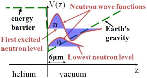
Figure 1: Schematic representation of the vertical potential and the first two states of a neutron above a horizontal mirror of liquid helium.

One can easily solve the one-dimensional Schrödinger equation for a neutron in the potential given by Eqs. (II) and (3) and shown in Fig. 1. The corresponding Hamiltonian is given by

$$\hat{H}_{0}=-\frac{\hbar^{2}\hat{\Delta}}{2m}+mgz+V_{0}\theta\left(-z\right),$$ (4)

where $\hat{\Delta}=\bm{\nabla}^{2}$ is the Laplace operator, $\bm{\nabla}$ is the gradient operator, and $\theta\left(x\right)$ is the step function [$\theta\left(x\right)=1$ for $x>0$ and $\theta\left(x\right)=0$ for $x\leq 0$]. The $x$, $y$ and $z$ coordinates separate in this equation, and the neutron wave function is given by a product

$$\psi\left(\mathbf{r}\right)=\psi_{\parallel}\left(\mathbf{r}_{||}\right)\,\psi_{\perp}\left(z\right),$$ (5)

where $\mathbf{r}_{||}=\left(x,y\right)$ is the 2D coordinate vector along the surface, while $\mathbf{r}=\left(x,y,z\right)$ stands for the 3D coordinate vector. In the $x$-$y$ plane, the neutron wave function is given by a normalized plane wave,

$$\psi_{\parallel}\left(\mathbf{r}_{||}\right)=S^{-1/2}\exp\left(i\mathbf{p}_{||}\mathbf{r}_{||}/\hbar\right),$$ (6)

where $S$ is the He surface area, and $\mathbf{p}_{||}$ is the 2D neutron momentum along the surface. For $z<0$ we can neglect the weak gravitational potential given by Eq. (3) as compared to the much stronger potential wall given by Eq. (II). The $z$-dependent part of the neutron wave function in this region is then approximately given by

$$\psi_{\perp}\left(z\right)=\psi_{\perp}\left(0\right)\exp\left(\kappa z\right)\qquad\left(z<0,\ E_{\perp}<V_{0}\right),$$ (7)

where $\kappa=ik_{\perp}=\sqrt{2m\left(V_{0}-E_{\perp}\right)}/\hbar$, and $E_{\perp}$ is the neutron kinetic energy along the $z$-axis. For $E_{\perp}\ll V_{0}$, $\kappa_{0}\equiv\sqrt{2mV_{0}}/\hbar\approx 2.4\times 10^{5}$ cm^-1, i.e. the neutron penetration depth into the liquid helium is

$$\kappa_{0}^{-1}\approx 33\ \mathrm{nm}.$$ (8)

For $z>0$, the neutron wave function is given by

$$\psi_{\perp}\left(z\right)=C\,\mathrm{Ai}\left[\left(z-E_{\perp}/mg\right)/z_{0}\right]\qquad\left(z>0\right),$$ (9)

where $C$ is a normalization coefficient, $\mathrm{Ai}\left(x\right)$ is the Airy function, and

$$z_{0}\equiv\left(\hbar^{2}/2m^{2}g\right)^{1/3}=5.87\ \mathrm{\mu m}$$ (10)

is a characteristic length scale of the neutron wave function in low energy states. For $z>E_{\perp}/mg$ the wave function given in Eq. (9) decreases exponentially. For $E_{\perp}<V_{0}$ the energy spectrum of the $z$-axis motion of a neutron above the liquid-helium surface is quantized. The eigenvalues of energy are given by the boundary condition at $z=0$, i.e.

$$\frac{\psi_{\perp}^{\prime}\left(0\right)}{\psi_{\perp}\left(0\right)}=\kappa=\frac{\sqrt{2m\left(V_{0}-E_{\perp}\right)}}{\hbar}=\frac{\mathrm{Ai}^{\prime}\left(-u\right)}{z_{0}\mathrm{Ai}\left(-u\right)},$$ (11)

where the prime indicates the derivative, and

$$u\equiv E_{\perp}/mgz_{0}.$$ (12)

Equation (11) for finite $V_{0}$ can be solved only numerically. A characteristic scale of separations between lowest energy levels is given by $mgz_{0}=\left(\hbar^{2}mg^{2}/2\right)^{1/3}=0.96\times 10^{-24}\ \mathrm{erg}=0.6$ peV.

In the limit $V_{0}\rightarrow\infty$ the energy levels are given by

$$E_{n}=mgz_{0}\alpha_{n+1},~{}n=0,1,...,$$ (13)

where $-\alpha_{n+1}$ are the zeros of the Airy function,

$$\alpha_{1}=2.338,\quad\alpha_{2}=4.088,\quad\alpha_{3}=5.521,\quad\alpha_{4}=6.787.$$ (14)

For $n\gg 1$,

$$\alpha_{n}\approx\left(3\pi n/2\right)^{2/3}-\left(\pi^{2}/96n\right)^{1/3}.$$ (15)

Note that this expression provides a highly accurate approximation even for small $n$: for $\alpha_{1}$ the error is only $\left|\Delta\alpha/\alpha\right|\approx 0.0018$, and further decreases for $n>1$, e.g., $\left|\Delta\alpha/\alpha\right|\approx 0.0005$ for $\alpha_{2}$.

For finite $V_{0}$, Eq. (11) can be rewritten as

$$\mathrm{Ai}^{\prime}\left(-u\right)=\mathrm{Ai}\left(-u\right)\sqrt{\eta_{0}-u},$$ (16)

using the dimensionless constant

$$\eta_{0}\equiv V_{0}/mgz_{0}=3.078\times 10^{4},$$ (17)

evaluated on the r.h.s. for $V_{0}$ of superfluid He. Eqs. (16) and (17) give the following values of $\alpha_{n+1}^{\mathrm{He}}=E_{n}/mgz_{0}$ of the discrete energy of a neutron above the He mirror:

$$\alpha_{1}^{\mathrm{He}}=2.332,\quad\alpha_{2}^{\mathrm{He}}=4.082,\quad\alpha_{3}^{\mathrm{He}}=5.515,\quad\alpha_{4}^{\mathrm{He}}=6.781.$$ (18)

These values are indeed very close to the values $\alpha_{n}$ for $V_{0}\rightarrow\infty$ [compare Eq. (14)], because $\eta_{0}\gg 1$. The neutron wave functions above liquid He are also very close to those for $V_{0}\rightarrow\infty$, except for a region close to $z=0$, where they acquires values $\psi_{\perp n}\left(0\right)=C_{n}\,\mathrm{Ai}\left(-\alpha_{n+1}^{\mathrm{He}}\right)$ which are small but finite, since $\alpha_{n+1}^{\mathrm{He}}\approx\alpha_{n+1}$. For the $n$-th energy level the normalization coefficient is given by

$$\frac{1}{C_{n}^{2}} = \int_{0}^{\infty}dz\left[\left|\mathrm{Ai}\left(\frac{z}{z_{0}}-\alpha_{n+1}^{\mathrm{He}}\right)\right|^{2}+\left|\mathrm{Ai}\left(-\alpha_{n+1}^{\mathrm{He}}\right)\right|^{2}e^{-2\kappa z}\right]$$ (19)

$$= z_{0}\int_{0}^{\infty}dx\left|\mathrm{Ai}\left(x-\alpha_{n+1}^{\mathrm{He}}\right)\right|^{2}+\frac{\left|\mathrm{Ai}\left(-\alpha_{n+1}^{\mathrm{He}}\right)\right|^{2}}{2\kappa}.$$

The first three normalization coefficients are given by $C_{0}\approx 1.4261/\sqrt{z_{0}}\approx 59\ \mathrm{cm}^{-1/2}$, $C_{1}\approx 51.3\ \mathrm{cm}^{-1/2}$, $C_{2}\approx 47.8\ \mathrm{cm}^{-1/2}$. Using the values $\mathrm{Ai}\left(-\alpha_{1}^{\mathrm{He}}\right)\approx 0.004$, $\mathrm{Ai}\left(-\alpha_{2}^{\mathrm{He}}\right)\approx-0.0045$, and $\mathrm{Ai}\left(-\alpha_{3}^{\mathrm{He}}\right)\approx 0.0048$, this gives $\psi_{\perp 0}\left(0\right)\approx 0.236\ \mathrm{cm}^{-1/2}$, $\psi_{\perp 1}\left(0\right)\approx-0.231\ \mathrm{cm}^{-1/2}$, $\psi_{\perp 2}\left(0\right)\approx 0.23\ \mathrm{cm}^{-1/2}$, etc. These values will be used further below.

In the subsequent sections we consider the stability of a neutron in a bound surface state against various scattering processes. Note that we deal here with a rather unfamiliar scattering problem in that the kinetic energy of the neutron parallel to the surface may be many orders of magnitude greater than the binding energies in the perpendicular direction. We calculate the temperature-dependent scattering rates $w_{\mathrm{vap}}$, $w_{\mathrm{rip}}$ and $w_{\mathrm{sur}}$ due to ⁴He atoms in the vapour above the surface, due to waves on the helium surface, called ripplons, and due to excitations called surfons, respectively.

III Scattering of neutrons in surface states by helium vapor

⁴He vapor atoms can be considered as point-like impurities with interaction potential given by Eq. (1). The momentum distribution of the vapor atoms is given by the Bose distribution CommentBoltzmann ,

$$N_{P}=\exp\left(\frac{\mu-E_{\mathrm{He}}}{k_{\mathrm{B}}T}\right),$$ (20)

where $k_{\mathrm{B}}=1.38\times 10^{-16}\ \mathrm{erg/K}$ is the Boltzmann constant, $\mu/k_{\mathrm{B}}=-7.17\ \mathrm{K}$ is the chemical potential of liquid ⁴He (evaporation energy of a ⁴He atom) for $T\rightarrow 0$, and $E_{\mathrm{He}}=\mathbf{P}^{2}/2M$ is the kinetic energy of a ⁴He atom with momentum $\mathbf{P}$. The total atom concentration in the vapor is given by the integrated momentum distribution, i.e.

$$N_{\mathrm{vap}}=\left(\frac{Mk_{\mathrm{B}}T}{2\pi\hbar^{2}}\right)^{3/2}\exp\left(\frac{\mu}{k_{\mathrm{B}}T}\right),$$ (21)

where $M=6.7\times 10^{-24}\ \mathrm{g}$ is the atomic ⁴He mass. Because of the energy-momentum conservation, the neutron scattering rate depends on the initial neutron state and on ⁴He atom momentum. We assume the initial neutron state to be given by the lowest energy level along the $z$-axis and by the momentum $\mathbf{p}_{||}=\left\{p_{x},p_{y}\right\}$ parallel to the helium surface, corresponding to the total neutron energy

$$K=p_{||}^{2}/2m+E_{0}.$$ (22)

In typical experiments with UCN, $K\approx p_{||}^{2}/2m\sim 10^{-7}\ \mathrm{eV}\gg E_{0}\sim 10^{-12}\ \mathrm{eV}$. The typical initial momentum $\mathbf{P}$ of a He atom is larger than the neutron momentum by still more than one order of magnitude, because its average kinetic energy $\bar{E}_{\mathrm{He}}=\left(3/2\right)k_{\mathrm{B}}T\sim 10^{-4}$ eV. Below [see Eq. (34)] we will see that, as $p_{||}\rightarrow 0$, the neutron-He scattering rate $w_{\mathrm{vap}}$ remains finite, and we can neglect $p_{||}/P\ll 1$ in the calculation of this rate.

III.1 Matrix elements

The initial neutron wave function is given by Eqs. (5), (6) and (9). Since the typical neutron out-of-plane kinetic energy after scattering by a He atom of the vapor is much larger than $E_{0}$, and mostly even larger than $V_{0}$ given in Eq. (II), the final neutron wave function is close to the three-dimensional plane wave with momentum $\mathbf{p}^{\prime}$, normalized to one particle in the whole volume $V$:

$$\psi^{\prime}=\exp\left(i\mathbf{p}^{\prime}\mathbf{r}/\hbar\right)/\sqrt{V}.$$ (23)

The initial He-atom wave function is$\ \Psi=\exp\left(i\mathbf{Pr}/\hbar\right)$, and the final He wave function is $\Psi^{\prime}=\exp\left(i\mathbf{P}^{\prime}\mathbf{r}/\hbar\right)$. The matrix element of the interaction potential (1) is given by

$$T_{\mathrm{if}} = \int d^{3}\mathbf{r}\bm{\,}\psi_{\perp 0}\left(z\right)\psi_{\parallel}\left(\mathbf{r}_{||}\right)\psi^{\prime}\left(\mathbf{r}\right)\times$$ (24)

$$\int d^{3}\mathbf{R}\exp\left(\frac{i\left(\mathbf{P}-\mathbf{P}^{\prime}\right)\bm{\mathbf{R}}}{\hbar}\right)U\,\delta^{(3)}\left(\mathbf{r}-\mathbf{R}\right)$$

$$= U\,\int\frac{d^{3}\mathbf{R}}{\sqrt{SV}}\psi_{\perp 0}\left(z_{\mathrm{He}}\right)\exp\left(\frac{i\Delta\mathbf{P}_{\mathrm{tot}}\bm{\mathbf{R}}}{\hbar}\right),$$

where $\Delta\mathbf{P}_{\mathrm{tot}}\approx\mathbf{P}-\mathbf{P}^{\prime}+\mathbf{p}_{||}-\mathbf{p}^{\prime}$ is the change of total momentum, $\mathbf{R}$ is the coordinate of the He nucleus, and $\psi_{\perp 0}\left(z\right)=C_{0}\,\mathrm{Ai}\left[\left(z-E_{0}/mg\right)/z_{0}\right]$ according to Eq. (9). Introducing $\tilde{u}\equiv z/z_{0}$ and performing the integration over $d^{2}\mathbf{R}_{\parallel}$ in Eq. (24) using the identity

$$\int d^{2}\mathbf{R}_{\parallel}\exp\left(i\Delta\mathbf{P}_{\mathrm{tot}\parallel}\bm{\mathbf{R}}_{\parallel}/\hbar\right)=\left(2\pi\hbar\right)^{2}\delta^{(2)}\left(\Delta\mathbf{P}_{\mathrm{tot}||}\right),$$ (25)

one can rewrite $T_{\mathrm{if}}$ as

$$T_{\mathrm{if}}=\frac{U\,\left(2\pi\hbar\right)^{2}\delta^{(2)}\left(\Delta\mathbf{P}_{\mathrm{tot}||}\right)}{\sqrt{SV/z_{0}}}I,$$ (26)

where the remaining integral is

$$I\equiv 1.4261\int_{0}^{\infty}d\tilde{u}\,\,\mathrm{Ai}\left(\tilde{u}-\alpha_{1}\right)\exp\left(\frac{i\Delta p_{z}\bm{\,}\tilde{u}}{\hbar/z_{0}}\right).$$

We calculate this integral approximately by replacing the normalized Airy function $f\left(\tilde{u}\right)\equiv 1.4261\mathrm{Ai}\left(\tilde{u}-\alpha_{1}\right)$ by a simpler form, also normalized, that is a close approximation, i.e.$\ f\left(\tilde{u}\right)\approx\exp\left[-\left(\tilde{u}-\tilde{u}_{0}\right)^{2}/2\right]/\pi^{1/4}$, where $\tilde{u}_{0}\approx 1.5$. Then,

$$I = \int_{0}^{\infty}d\tilde{u}\,\,f\left(\tilde{u}\right)\exp\left(\frac{i\Delta p_{z}\bm{\,}\tilde{u}}{\hbar/z_{0}}\right)$$ (27)

$$\approx \int_{-\infty}^{\infty}\frac{d\tilde{u}\,}{\pi^{1/4}}\,\exp\left[\frac{-\left(\tilde{u}-\tilde{u}_{0}\right)^{2}}{2}+\frac{i\Delta p_{z}\bm{\,}\tilde{u}}{\hbar/z_{0}}\right]$$

$$= \pi^{1/4}\sqrt{2}\exp\left[\frac{i\Delta p_{z}\bm{\,}\tilde{u}_{0}}{\hbar/z_{0}}-\frac{1}{2}\left(\frac{\Delta p_{z}\bm{\,}}{\hbar/z_{0}}\right)^{2}\right].$$

Below we need only the square of the absolute value of the matrix element $T_{\mathrm{if}}$. The square of the $\delta$-function in $\left|T_{\mathrm{if}}\right|^{2}$ should be treated as

$$\left[\left(2\pi\hbar\right)^{2}\delta^{(2)}\left(\Delta\mathbf{P}_{\mathrm{tot}||}\right)\right]^{2}=S\left(2\pi\hbar\right)^{2}\delta^{(2)}\left(\Delta\mathbf{P}_{\mathrm{tot}||}\right),$$ (28)

because it comes from the extra integration over the coordinate $\mathbf{r}_{i||}$: $\int d^{2}\mathbf{r}_{i\parallel}=S$. Indeed, substituting Eq. (25) to the l.h.s. of Eq. (28) we obtain

$$\left(2\pi\hbar\right)^{2}\delta^{(2)}\left(\Delta\mathbf{P}_{\mathrm{tot}||}\right)\int d^{2}\mathbf{r}_{i\parallel}\exp\left(\frac{i\Delta\mathbf{P}_{\mathrm{tot}\parallel}\mathbf{r}_{i\parallel}}{\hbar}\right)=$$

$$=\left(2\pi\hbar\right)^{2}\delta^{(2)}\left(\Delta\mathbf{P}_{\mathrm{tot}||}\right)\int d^{2}\mathbf{r}_{i\parallel}=S\left(2\pi\hbar\right)^{2}\delta^{(2)}\left(\Delta\mathbf{P}_{\mathrm{tot}||}\right).$$

Substituting Eq. (27) to Eq. (26) and using Eq. (28), we obtain

$$\left|T_{\mathrm{if}}\right|^{2}\approx\frac{U^{2}\,\left(2\pi\hbar\right)^{3}\delta^{(2)}\left(\Delta\mathbf{P}_{\mathrm{tot}||}\right)}{V\sqrt{\pi}\hbar/z_{0}}\exp\left[-\left(\frac{\Delta p_{z}\bm{\,}}{\hbar/z_{0}}\right)^{2}\right].$$

Since $\hbar/z_{0}\ll P$, using the identity

$$\delta\left(x\right)=\lim_{\epsilon\rightarrow 0}\left[\frac{1}{\epsilon\sqrt{\pi}}\exp\left(-\frac{x^{2}}{\epsilon^{2}}\right)\right],$$

we rewrite $\left|T_{\mathrm{if}}\right|^{2}$ as

$$\left|T_{\mathrm{if}}\right|^{2}\approx U^{2}\,\left(2\pi\hbar\right)^{3}\delta^{(3)}\left(\Delta\mathbf{P}_{\mathrm{tot}}\right)/V.$$ (29)

III.2 Scattering rate

The scattering rate of a neutron with initial in-plane momentum $\mathbf{p}_{||}$ by a He atom with initial momentum $\mathbf{P}$ is given by the square of the matrix element (29) integrated over the final momenta $\mathbf{p}^{\prime}$ and $\mathbf{P}^{\prime}$ of the neutron and He atom, respectively (Fermi’s golden rule LL3 ):

$$w_{\mathbf{P}}=\frac{2\pi}{\hbar}\int\frac{d^{3}\mathbf{P}^{\prime}}{(2\pi\hbar)^{3}}\int\frac{Vd^{3}\mathbf{p}^{\prime}}{(2\pi\hbar)^{3}}\left|T_{\mathrm{if}}\right|^{2}\delta\left(\varepsilon-\varepsilon^{\prime}\right).$$ (30)

Here $\varepsilon\approx P^{2}/2M$ and $\varepsilon^{\prime}=P^{\prime 2}/2M+\left(\mathbf{p}-\mathbf{p}^{\prime}\right)^{2}/2m$ are the initial and final total energies of He-atom and neutron. The scattering rate is approximately independent of the initial neutron momentum $\mathbf{p}_{||}$, i.e., $w_{\mathbf{P}}\equiv w\left(\mathbf{p}_{||},\mathbf{P}\right)\approx w\left(\mathbf{P}\right)$, because $p_{||}\ll P$ can be neglected in Eq. (30). We now substitute Eq. (29) to Eq. (30). The integration over $\mathbf{p}^{\prime}$ cancels $\delta^{3}\left(\Delta\mathbf{P}_{\mathrm{tot}}\right)$ in Eq. (29), where $\Delta\mathbf{P}_{\mathrm{tot}}\approx\mathbf{P}-\mathbf{P}^{\prime}-\mathbf{p}^{\prime}$. After the integration over the angle $\phi$ between $\mathbf{P}$ and $\mathbf{P}^{\prime}$ we obtain

$$w_{\mathbf{P}} = \int\frac{P^{\prime 2}dP^{\prime}}{2\pi\hbar^{4}}\frac{mU^{2}}{PP^{\prime}}\times\,$$

$$\theta\left[2PP^{\prime}-\left|P^{2}\left(1-\frac{m}{M}\right)+P^{\prime 2}\left(1+\frac{m}{M}\right)\right|\right].$$

Using $M\approx 4m$, from Eq. (III.2) we obtain

$$w_{\mathbf{P}}\approx\int\frac{P^{\prime 2}dP^{\prime}}{2\pi\hbar^{4}}\frac{mU^{2}}{PP^{\prime}}\theta\left[8PP^{\prime}-3P^{2}-5P^{\prime 2}\right].$$ (32)

The integrand is nonzero when the inequality

$$5P^{\prime 2}-8PP^{\prime}+3P^{2}<0$$ (33)

is satisfied. The quadratic expression has two real roots, $P^{\prime}=P\left(4\pm 1\right)/5$, so that Eq. (33) is satisfied for $3/5<P^{\prime}/P<1$, thus defining the range of integration in Eq. (32), i.e.

$$w_{\mathbf{P}}=\int_{3P/5}^{P}\frac{P^{\prime}dP^{\prime}}{2\pi\hbar^{4}}\frac{mU^{2}}{P}=\frac{U^{2}Pm}{2\pi\hbar^{4}}\frac{8}{25}.$$ (34)

Finally, to obtain the total scattering rate as function of temperature one has to integrate Eq. (34) over the initial He-atom momentum $\mathbf{P}$, weighted with the distribution function $N_{P}$ of He vapor given by Eq. (20),

$$w_{\mathrm{vap}}\left(T\right) = \int\frac{d^{3}\mathbf{P}~{}N_{P}}{(2\pi\hbar)^{3}}w_{\mathbf{P}}$$

$$= \int\frac{P^{2}dP^{2}~{}}{(2\pi\hbar)^{3}}\frac{U^{2}}{\hbar^{4}}\frac{8m}{25}\exp\left(\frac{\mu-P^{2}/2M}{k_{\mathrm{B}}T}\right).$$

Introducing the new dimensionless variable $P^{2}/2Mk_{\mathrm{B}}T$ and performing the integration we obtain

$$w_{\mathrm{vap}}\left(T\right)=\frac{\left(2Mk_{\mathrm{B}}T\right)^{2}}{(2\pi\hbar)^{3}}\frac{U^{2}}{\hbar^{4}}\frac{8m}{25}\exp\left(\frac{\mu}{k_{\mathrm{B}}T}\right).$$ (35)

After substitution of Eq. (1) one obtains

$$w_{\mathrm{vap}}\left(T\right)=9.44\ \mathrm{s}^{-1}\times\left(T\left[\mathrm{K}\right]\right)^{2}\times\exp\left(\frac{-7.17}{T\left[\mathrm{K}\right]}\right).$$ (36)

Hence, $w_{\mathrm{vap}}\left(1\ \mathrm{K}\right)\approx 0.007\ \mathrm{s}^{-1}=(138\ \mathrm{s})^{-1}$, and the estimated mean scattering time of a neutron in the lowest level, as determined by He vapor only, is about $138$ s at $T=1$ K. Lowering the temperature diminishes the scattering rate more rapid than exponentially, e.g., $w_{\mathrm{vap}}\left(T=0.8\ \mathrm{K}\right)\approx 7.74\times 10^{-4}\ \mathrm{s}^{-1}=\left(21.53\text{ min}\right)^{-1}$, and $w_{\mathrm{vap}}\left(T=0.7\ \mathrm{K}\right)\approx 1.6\times 10^{-4}$ s^-1. The break-even with neutron decay is thus reached slightly above $0.8$ K.

IV Scattering from surface waves

IV.1 General information about ripplons

A quantum of a surface wave (ripplon) with momentum $\mathbf{q}$ induces a surface deformation along the $z$-axis, given by

$$\xi(\mathbf{r}_{\parallel},t)=\xi_{0q}\sin\left(\mathbf{qr}_{\parallel}-\omega_{q}t\right).$$ (37)

The dispersion relation of surface waves is given by LL6 ; Shikin

$$\omega_{q}^{2}=\frac{\alpha}{\rho}\left(q^{2}+\varkappa^{2}\right)q\tanh\left(qd\right),$$ (38)

where $\alpha\approx 0.354$ dyn/cm is the surface tension coefficient of superfluid ⁴He, $\rho\approx 0.145$ g/cm³ is its mass density, $d$ is the depth of the helium bath above a horizontal bottom wall, and $\varkappa^{2}=\left(g+f\right)\rho/\alpha$ with an additional force $f\propto d^{-4}$ due to the van-der-Waals attraction of helium to the bottom wall. The ripplon amplitude $\xi_{0q}$ in Eq. (37), normalized to one ripplon per surface area $S$, is given by Shikin ; SM ; CommentSW

$$\xi_{0q}=\left(\frac{\hbar q\tanh\left(qd\right)}{2S\,\rho\omega_{q}}\right)^{1/2}.$$ (39)

For a helium bath (in fact already for a thick helium film), $\varkappa=\sqrt{g\rho/\alpha}\approx 20$ cm^-1. The thermal ripplons with energy $\hbar\omega_{q}\approx k_{\mathrm{B}}T\approx 0.5$ K have the wave number $q\approx 1.2$ nm^-1, for which holds $q\gg\varkappa$ and $qd\gg 1$. Then the dispersion relation of ripplons is just the dispersion of capillary waves:

$$\omega_{q}\approx\sqrt{\alpha/\rho}q^{3/2},$$ (40)

and

$$\xi_{0q}\approx\left(\frac{\hbar}{2S\,\sqrt{\rho\alpha q}}\right)^{1/2}.$$ (41)

IV.2 Interaction Hamiltonian

To determine the influence of a periodic surface deformation on the neutron quantum state on the surface we have to separate two limits. The first, adiabatic limit appears when the surface oscillates so slowly that the neutron wave function adjusts to the instantaneous surface profile. The interaction potential in this limit is found in Appendix A, see Eq. (78), and can be rewritten as

$$\hat{H}_{\mathrm{int}}=\xi(\mathbf{r}_{\parallel},t)\left\{\left[\frac{\left(\hat{p}_{\parallel}+\hat{p}_{q}\right)^{2}-\hat{p}_{\parallel}^{2}}{2m}-\hbar\omega_{q}\right]\frac{\partial}{\partial z}+mg\right\},$$ (42)

where $\hat{p}_{\parallel}=-i\hbar\bm{\nabla}_{\parallel}$ and $\hat{p}_{q}=\hbar q$ are the momentum operators of the neutron and ripplon along the surface, respectively. This interaction term generalizes Eq. (7) of Ref. Abele/2010 , because it does not exclude coordinate-dependent surface perturbations. The expression in the square brackets in Eq. (42) is just the transfer of the total (neutron+ripplon) kinetic energy to the final neutron kinetic energy along the $z$-axis.

The opposite, anti-adiabatic or diabatic limit appears when the surface oscillates much faster than the characteristic frequency of the out-of-plane neutron motion, so that the neutron wave function does not adjust to the instantaneous surface profile. In this limit a surface wave affects the neutrons by creating an additional time- and coordinate-dependent periodic potential

$$V_{r}(\mathbf{r}_{\parallel},z)=\left\{\begin{array}[]{c}V_{0}~{}\text{at }0<z<\xi(\mathbf{r}_{\parallel},t)\text{ for }\xi(\mathbf{r}_{\parallel},t)>0\\ -V_{0}\text{ at }\xi(\mathbf{r}_{\parallel},t)<z<0\text{ for }\xi(\mathbf{r}_{\parallel},t)<0\end{array}\right..$$ (43)

The ripplon amplitude, given by Eqs. (39) or (41), for any reasonable value of $S$ is much less than the atomic scale and, even more, than the typical scale of the neutron wave function, given by $\kappa_{0}^{-1}\approx 33$ nm at $z<0$ [Eq. (8)]. Therefore, the potential in Eq. (43) can be approximated by

$$V_{r}(\mathbf{r})\equiv V_{r}(\mathbf{r}_{\parallel},z)\approx V_{0}\xi(\mathbf{r}_{\parallel},t)\delta\left(z\right).$$ (44)

IV.3 Crossover between adiabatic and diabatic limits and matrix elements

The diabatic-adiabatic crossover, corresponding to a change of the ripplon-neutron interaction Hamiltonian from Eq. (43) to Eq. (42), must take place when the ripplon frequency $\omega_{q}$ and the wave-vector $\mathbf{q}$ decrease. However, the estimate of the crossover frequency $\omega_{q\mathrm{c}}$ and the description of the system in the crossover regime is not a trivial problem. Similar problem appears in other condensed-matter systems and requires a special theoretical study (see, e.g., Refs. Eidel2013 ; Giamarchi2005 ; Dora2011 ; Feig1998 ; Ogawa1999 ).

One may, naively, define the crossover as the region where the ripplon frequency becomes comparable to the quasi-classical bouncing frequency of a neutron in the ground level in $z$-direction, i.e. when the ratio $\hbar\omega_{q}/E_{0}\sim 1$, where $E_{0}$ given by Eq. (13). This corresponds to the ripplon frequency

$$\omega_{q\mathrm{c}}\sim E_{0}/\hbar=915\ \mathrm{s}^{-1},$$ (45)

and to the ripplon wave number

$$q_{\mathrm{c}}\approx\left(\omega_{q\mathrm{c}}^{2}\rho/\alpha\right)^{1/3}=70\ \mathrm{cm}^{-1}>\varkappa.$$ (46)

However, such an estimate of the diabatic-adiabatic crossover has an important drawback: it does not depend on the value $V_{0}$ of the neutron potential inside helium. Generally, we expect that for $V_{0}\rightarrow 0$ and for non-zero $q$ and $\omega_{q}$ one can always apply Eq. (43), and for $V_{0}\rightarrow\infty$ one can always apply Eq. (42), which contradicts Eq. (45). The classical definition of the diabatic-adiabatic crossover, given by Eqs. (83) and (84) in Appendix B, has the same drawback.

A rigorous analysis of the adiabatic/diabatic crossover should be based on the solution of the Schrödinger equation for a neutron in the time-dependent potential given by Eqs. (71) and (72). One may approximately determine the criterion of adiabatic/diabatic crossover from the variational principle to minimize the neutron energy. This approach would be definitely correct for a time-independent potential. The lowest-level out-of-plane neutron wave function is chosen to minimize the neutron energy. In the adiabatic limit the energy loss is the kinetic and gravitational energy from Eq. (42), while in the diabatic limit it is the potential energy from Eq. (43). The first-order energy correction is given by the diagonal matrix elements of these two interaction potentials, or more precisely by the Hamiltonian in Eq. (72). If these diagonal matrix elements are nonzero, their comparison gives the crossover frequency. If these matrix elements vanish in the first order in $\xi$, one needs to calculate and compare the second-order corrections. Since $\int_{-\infty}^{\infty}dz\psi_{\perp 0}^{\ast}\left(z\right)\partial\psi_{\perp 0}\left(z\right)/\partial z=0$, and $\int\xi(\mathbf{r}_{\parallel},t)d^{2}\mathbf{r}_{||}=0$, the first-order (in $\xi$) diagonal matrix element of the adiabatic Hamiltonian in Eq. (42) vanishes. So does the diagonal matrix element of the diabatic Hamiltonian in Eq. (43) in the first-order in $\xi$, if $\mathbf{p}_{||}\neq\hbar\mathbf{q}$. Hence, to calculate the crossover frequency one needs to calculate the second-order energy corrections, which do not vanish. These corrections are determined, in particular (but not only), by the matrix elements of the neutron-ripplon interaction potentials in Eqs. (42) and (43). Therefore, for an estimate of the position (ripplon frequency) of the adiabatic/diabatic crossover the comparison of the matrix elements, given below, is more accurate than just the comparison of ripplon frequency with $E_{0}$. As we will see, the final result of the neutron-ripplon scattering rate is not sensitive to this crossover frequency, because the main contribution to this scattering rate comes from the ripplons with energy $\hbar\omega_{q}\sim V_{0}\gg\hbar\omega_{q\mathrm{c}}$, which corresponds to the far diabatic limit.

Therefore, a rough estimate of the crossover between diabatic and adiabatic limits is given by the ripplon frequency when two interaction Hamiltonians, given by Eqs. (43) and (42), become of the same order of magnitude. More precisely, we compare their matrix elements for the neutron transitions between lowest energy levels of their motion in $z$-direction. Thus defined, the diabatic-adiabatic crossover depends on $V_{0}$ and meets other general requirements, such as the adiabatic limit for $\omega_{q},q\rightarrow 0$. The matrix element $T_{\mathrm{if}}$ of the diabatic interaction potential in Eq. (44) for the transitions between two neutron states with initial wave function $\psi_{\perp}\left(z\right)$ and final wave function $\psi_{\perp}^{\prime}\left(z\right),$ written explicitly in Eqs. (5)-(9), is given by

$$T_{\mathrm{if}}=\int\frac{d^{3}\mathbf{r}\bm{\,}}{S}\psi_{\perp}\left(z\right)\psi_{\perp}^{\prime\ast}\left(z\right)\exp\left(i\mathbf{r}_{||}\frac{\mathbf{p}_{||}-\mathbf{p}_{\parallel}^{\prime}\,}{\hbar}\right)V_{0}\xi(\mathbf{r}_{\parallel})\delta\left(z\right).$$

The integral over $z$ cancels $\delta\left(z\right)$, while after substituting Eq. (37) the integration over $\mathbf{r}_{||}$ gives $\left(2\pi\hbar\right)^{2}\delta^{(2)}\left(\Delta\mathbf{p}_{\mathrm{tot}||}\right)$, where $\Delta\mathbf{p}_{\mathrm{tot}||}=\hbar\mathbf{q}+\mathbf{p}_{||}-\mathbf{p}_{\parallel}^{\prime}$ is the change of the total in-plane momentum of the ripplon+neutron system. As a result we obtain

$$T_{\mathrm{if}}=V_{||}V_{0,n}\,.$$ (47)

The factor

$$V_{||}=S^{-1}\left(2\pi\hbar\right)^{2}\delta^{(2)}\left(\Delta\mathbf{p}_{\mathrm{tot}||}\right)$$ (48)

is due to the in-plane part $\psi_{\parallel}\left(\mathbf{r}_{||}\right)$ of the neutron wave function, given by Eq. (6), and

$$V_{0,n}=V_{0}\xi_{0q}\psi_{\perp 0}^{\ast}\left(0\right)\psi_{\perp n}\left(0\right)$$ (49)

comes from its out-of-plane part $\psi_{\perp}\left(z\right)$. The squared modulus of the matrix element in Eq. (47) follows as

$$\left|T_{\mathrm{if}}\right|^{2}=\frac{\left(2\pi\hbar\right)^{2}\delta^{(2)}\left(\Delta\mathbf{p}_{\mathrm{tot}||}\right)}{S}\left|\psi_{\perp}\left(0\right)\psi_{\perp}^{\prime\ast}\left(0\right)V_{0}\xi_{0q}\right|^{2},$$ (50)

where we again have used Eq. (28).

The matrix elements of the adiabatic interaction potential in Eq. (42) for $\xi(\mathbf{r}_{\parallel},t)$ given by Eq. (37) are

$$\hat{H}_{k,n}=V_{||}\xi_{0q}\left(E_{k}-E_{n}\right)Q_{k,n},$$ (51)

where $V_{||}$ is again given by Eq. (48) and

$$Q_{k,n}=\int_{0}^{\infty}dz\psi_{\perp k}^{\ast}\left(z\right)\frac{d\psi_{\perp n}^{\ast}\left(z\right)}{dz}.$$ (52)

The first values of $Q_{k,n}$ are given in Table I of Ref. Abele/2010 , e.g., $Q_{0,1}=0.09742\ \mathrm{\mu m}^{-1}$, $Q_{0,2}=-0.05355\ \mathrm{\mu m}^{-1}$, $Q_{0,3}=0.03831\ \mathrm{\mu m}^{-1}$, $Q_{0,4}=-0.0304\ \mathrm{\mu m}^{-1}$. Substituting these values we obtain for the first levels the ratio $V_{0,n}/\hat{H}_{0,n}\approx 1$ at

$$\omega_{q\mathrm{c}}\approx 10^{3}\ \mathrm{s}^{-1}.$$ (53)

By chance, the diabatic-adiabatic crossover condition, defined as $V_{0,n}\sim\hat{H}_{0,n}$, is close to the value quoted in Eq. (45).

Below, we consider mainly the neutron-ripplon interaction in the diabatic limit, corresponding to the ripplon frequency $\omega_{q}>\omega_{q\mathrm{c}}$ and the interaction potential given by Eq. (44), because it deals with much larger phase space of ripplons and because, as we will see later, the main contribution to the neutron-ripplon scattering rate comes from the ripplons with energy $\hbar\omega_{q}\sim V_{0}\gg\hbar\omega_{q\mathrm{c}}$.

The scattering rate $w_{\mathrm{rip}}$ of a neutron with initial in-plane momentum $\mathbf{p}_{||}$ on ripplons is determined by two processes: the absorption and the emission of a ripplon with wave vector $\mathbf{q}$ and energy $\hbar\omega_{q}$,

$$w_{\mathrm{rip}}=w_{\mathrm{abs}}+w_{\mathrm{em}}.$$ (54)

Since for typical ⁴He temperatures $k_{\mathrm{B}}T$ is much larger than the initial neutron energy $K$, the populations of ripplon states with relevant energies are $N_{q}\gtrsim 1$ or even $N_{q}\gg 1$. The phase volume of an absorbed ripplon is much larger than that of an emitted ripplon, because the energy of the latter is limited to the initial kinetic energy of the neutron, $K\ll k_{\mathrm{B}}T$. Hence, one could expect that the ripplon-neutron scattering rate is dominated by ripplon absorption, so that $w_{\mathrm{rip}}\approx w_{\mathrm{abs}}$. However, because of a low-energy divergence of $w_{\mathrm{rip}}$ (see below), the emission of low-energy ripplons with energies $\hbar\omega_{q}\ll K$ may also be important, and we therefore consider both these processes.

IV.4 Absorption of ripplons

The absorption scattering rate $w_{\mathrm{abs}}$ of a neutron with initial in-plane momentum $\mathbf{p}_{||}$ in the discrete vertical level with energy $E_{0}$ is given by Fermi’s golden rule,

$$w_{\mathrm{abs}}=\frac{2\pi}{\hbar}\int\frac{N_{q}Sd^{2}\mathbf{p}_{q}}{(2\pi\hbar)^{2}}\int\frac{Sd^{2}\mathbf{p}_{\parallel}^{\prime}}{(2\pi\hbar)^{2}}\sum_{n}\left|T_{\mathrm{if}}\right|^{2}\delta\left(\varepsilon-\varepsilon^{\prime}\right),$$ (55)

where $\mathbf{p}_{q}\equiv\hbar\mathbf{q}$ is the ripplon momentum, and $\mathbf{p}_{\parallel}^{\prime}$ and $n$ are the in-plane momentum and out-of-plane quantum number of the final neutron state, respectively.

$$N_{q}=\left[\exp\left(\hbar\omega_{q}/k_{\mathrm{B}}T\right)-1\right]^{-1}$$ (56)

is the Bose distribution function of ripplons with energy $\hbar\omega_{q}$ and with zero chemical potential. The matrix element $\left|T_{\mathrm{if}}\right|$ is given by Eq. (50) and the initial total energy by

$$\varepsilon=\hbar\omega_{q}+\mathbf{p}_{\parallel}^{2}/2m+E_{0}.$$ (57)

The final energy $\varepsilon^{\prime}=\mathbf{p}_{\parallel}^{\prime 2}/2m+E_{n}$, after using the in-plane momentum conservation expressed by the $\delta$-function in Eq. (50), can be rewritten as

$$\varepsilon^{\prime}=\frac{p_{\parallel}^{2}+p_{q}^{2}+2p_{q}p_{\parallel}\cos\phi}{2m}+E_{n},$$ (58)

where $\phi$ is the angle between $\mathbf{p}_{\parallel}$ and $\mathbf{p}_{q}$. The integration over the component $\mathbf{p}_{\parallel}^{\prime}$ of the final neutron momentum parallel to the surface cancels the $\delta$-function in Eq. (50). After substitution of Eqs. (50), (57) and (58) to Eq. (55) we obtain

$$w_{\mathrm{abs}} = \int\frac{N_{q}Sp_{q}dp_{q}d\phi}{2\pi\hbar^{3}}\sum_{n}\left|\psi_{\perp 0}\left(0\right)\psi_{\perp n}^{\ast}\left(0\right)V_{0}\xi_{0q}\right|^{2}$$ (59)

$$\times\delta\left(\hbar\omega_{q}-\Delta E_{n}-\frac{p_{q}^{2}+2p_{q}p_{\parallel}\cos\phi}{2m}\right),$$

where $\Delta E_{n}=E_{n}-E_{0}\approx E_{n}$ is the change of the out-of-plane neutron energy after the ripplon absorption. The integration over $\phi$ cancels the $\delta$-function in Eq. (59) and gives

$$w_{\mathrm{abs}}=\int_{0}^{\infty}\frac{N_{q}Sp_{q}dp_{q}}{\pi\hbar^{3}}\sum_{n}\frac{\left|\psi_{\perp 0}\left(0\right)\psi_{\perp n}^{\ast}\left(0\right)V_{0}\xi_{0q}\right|^{2}}{\sqrt{a^{2}-\left(b-\Delta E_{n}\right)^{2}}},$$ (60)

where $a\equiv p_{\parallel}p_{q}/m$ and $b\equiv\hbar\omega_{q}-p_{q}^{2}/2m$.CommentI We estimate this integral in the Appendix C. This calculation gives the upper estimate of $w_{\mathrm{abs}}$ [see Eqs. (95), (101) and (105)] of

$$w_{\mathrm{abs}}^{\mathrm{up}}\approx w_{>}^{\mathrm{up}}+w_{<}^{\mathrm{up}}+w_{\ll}^{\mathrm{up}}\approx 7\times 10^{-5}\times T\left[\mathrm{K}\right]~{}\mathrm{s}^{-1}.$$ (61)

This corresponds to a mean neutron scattering time due to ripplon absorption of $\tau_{\mathrm{rip}}>4$ hours even at $T=1$ K.

IV.5 Emission of ripplons

The rate of emission of a ripplon by a surface-state neutron with momentum $\mathbf{p}_{\parallel}$ is given by Fermi’s golden rule, similar to Eq. (55):

$$w_{\mathrm{em}}=\frac{2\pi}{\hbar}\int\frac{N_{q}^{\prime}Sd^{2}\mathbf{p}_{q}}{(2\pi\hbar)^{2}}\int\frac{Sd^{2}\mathbf{p}^{\prime}}{(2\pi\hbar)^{2}}\sum_{n}\left|T_{\mathrm{if}}\right|^{2}\delta\left(\varepsilon-\varepsilon^{\prime}\right).$$ (62)

Here, $\mathbf{p}_{q}\equiv\hbar\mathbf{q}$ is now the emitted-ripplon momentum, $\mathbf{p}^{\prime}=\mathbf{p}_{\parallel}-\mathbf{p}_{q}$ is the in-plane neutron momentum after emission of the ripplon,

$$N_{q}^{\prime}=1+\left[\exp\left(\hbar\omega_{q}/k_{\mathrm{B}}T\right)-1\right]^{-1},$$ (63)

is the ripplon population, $\varepsilon\approx\mathbf{p}_{\parallel}^{2}/2m$ is the initial total energy, and

$$\varepsilon^{\prime}=\frac{p_{\parallel}^{2}+p_{q}^{2}-2p_{q}p_{\parallel}\cos\phi}{2m}+E_{n}+\hbar\omega_{q},$$

is the final total energy. The matrix element is given by Eq. (50). The integration over $\mathbf{p}^{\prime}$ in Eq. (62) cancels the $\delta$-function in the matrix element,

$$w_{\mathrm{em}} = \int\frac{SN_{q}^{\prime}p_{q}dp_{q}}{2\pi\hbar^{3}}\sum_{n}\left|\psi_{\perp}\left(0\right)\psi_{\perp}^{\prime\ast}\left(0\right)V_{0}\xi_{0q}\right|^{2}$$ (64)

$$\times\int_{0}^{2\pi}d\phi\delta\left(\frac{p_{q}^{2}-2p_{q}p_{\parallel}\cos\phi}{2m}+E_{n}+\hbar\omega_{q}\right).$$

The integration over the angle $\phi$ between $\mathbf{p}_{\parallel}$ and $\mathbf{p}_{q}$ in Eq. (64) is similar to that in the preceding subsection in Eq. (59) and gives

$$w_{\mathrm{em}}=\int_{0}^{p_{\mathrm{em}}^{\max}}\frac{SN_{q}p_{q}dp_{q}}{\pi\hbar^{3}}\sum_{n}\frac{\left|\psi_{\perp}\left(0\right)\psi_{\perp}^{\prime\ast}\left(0\right)V_{0}\xi_{0q}\right|^{2}}{\sqrt{a^{2}-\left(b_{1}+\Delta E_{n}\right)^{2}}},$$ (65)

where $a\equiv p_{\parallel}p_{q}/m$ as in the previous subsection, and $b_{1}=\hbar\omega_{q}+p_{q}^{2}/2m$. The integrand is real when $0\leq\Delta E_{n}\approx E_{n}\leq a-b_{1}=p_{\parallel}p_{q}/m-\hbar\omega_{q}-p_{q}^{2}/2m$. This can be satisfied when $a-b_{1}>0$, which for $p_{\parallel}^{2}/2m=100$ neV gives $p_{q}<p_{\mathrm{em}}^{\max}=\hbar q_{\mathrm{em}}^{\max}$ with $q_{\mathrm{em}}^{\max}\approx 6.5\times 10^{4}$ cm^-1. The maximum value of $a-b_{1}$ is $\sim 3\ \mathrm{neV}\ll V_{0}=18.5$ neV. Hence, for the emission of ripplons, $E_{n}\ll V_{0}$, and we may use Eqs. (13), (15) and (102). In addition, instead of three intervals of parameters for the ripplon absorption, we only need to consider one interval. Substituting Eqs. (40), (41) and the upper estimate of $\left|\psi_{\perp}^{\prime}\left(0\right)\right|^{2}\leq\left|\psi_{\perp 0}\left(0\right)\right|^{2}$ to Eq. (65), we obtain an upper estimate $w_{\mathrm{em}}^{\mathrm{up}}$ for $w_{\mathrm{em}}$:

$$w_{\mathrm{em}}^{\mathrm{up}} \approx \int_{0}^{p_{\mathrm{em}}^{\max}}\frac{k_{\mathrm{B}}Tp_{q}dp_{q}}{2\pi\hbar\alpha p_{q}^{2}}\int\frac{dn\left|\psi_{\perp 0}^{2}\left(0\right)V_{0}\right|^{2}}{\sqrt{a^{2}-\left(b_{1}+E_{n}\right)^{2}}}$$

$$= \int\frac{k_{\mathrm{B}}Tdp_{q}}{\pi^{2}\hbar^{2}\alpha p_{q}}\frac{\left|\psi_{\perp 0}^{2}\left(0\right)V_{0}\right|^{2}}{g\sqrt{2m}}\int_{0}^{a-b_{1}}\frac{\sqrt{E_{n}}dE_{n}}{\sqrt{a^{2}-\left(b_{1}+E_{n}\right)^{2}}}.$$

This integral resembles the one in Eq. (103): the only difference is the sign of $E_{n}$ in the denominator and, consequently, a different upper integration limit. We may give an upper estimate of this integral by replacing $\sqrt{E_{n}}$ by its maximum value $\sqrt{a-b_{1}}$ in the integrand and by replacing the lower limit by $-b_{1}$ in Eq. (IV.5). This gives

$$w_{\mathrm{em}}^{\mathrm{up}} \approx \int\frac{k_{\mathrm{B}}Tdp_{q}}{\pi^{2}\hbar^{2}\alpha p_{q}}\frac{\left|\psi_{\perp 0}^{2}\left(0\right)V_{0}\right|^{2}}{g\sqrt{2m}}\int_{-b_{1}}^{a-b_{1}}\frac{\sqrt{a-b_{1}}dE_{n}}{\sqrt{a^{2}-\left(b_{1}+E_{n}\right)^{2}}}$$

$$= \int_{0}^{p_{\mathrm{em}}^{\max}}\frac{k_{\mathrm{B}}Tdp_{q}}{\pi\hbar^{2}\alpha p_{q}}\frac{\left|\psi_{\perp 0}^{2}\left(0\right)V_{0}\right|^{2}}{2g\sqrt{2m}}\sqrt{\frac{p_{\parallel}p_{q}}{m}-\hbar\omega_{q}-\frac{p_{q}^{2}}{2m}}.$$

The integral converges. Neglecting $p_{q}^{2}/2m\ll\hbar\omega_{q}$ and changing the integration variable to $\sqrt{p_{q}}$ we finally obtain

$$w_{\mathrm{em}}^{\mathrm{up}}\approx\frac{k_{\mathrm{B}}T}{\pi\hbar^{2}\alpha}\frac{\left|\psi_{\perp 0}^{2}\left(0\right)V_{0}\right|^{2}}{g\sqrt{2m}}\frac{2}{3}\left(\frac{p_{\parallel}}{m}\right)^{3/2}\sqrt{\frac{\rho\hbar}{\alpha\,}}.$$ (67)

The rate of ripplon emission depends on the initial neutron momentum $p_{\parallel}$. At $K=p_{\parallel}^{2}/2m=100$ neV Eq. (67) gives

$$w_{\mathrm{em}}^{\mathrm{up}}\approx 2\times 10^{-5}\ \mathrm{s}^{-1}\times T\left[\mathrm{K}\right].$$ (68)

Combining Eqs. (61) and (68) we obtain an upper estimate for the total scattering rate of a surface neutron in the lowest energy level $E_{0}$ by ripplons:

$$w_{\mathrm{rip}}^{\mathrm{up}}=w_{\mathrm{abs}}^{\mathrm{up}}+w_{\mathrm{em}}^{\mathrm{up}}\approx 9\times 10^{-5}\ \mathrm{s}^{-1}\times T\left[\mathrm{K}\right].$$ (69)

This rate corresponds to a mean neutron scattering time due to the ripplons of $\tau_{\mathrm{rip}}>3$ hours even at $T=1$ K.

V Other neutron scattering processes

V.1 Scattering of surface neutrons by bulk phonons

The scattering of ultra-cold neutrons inside superfluid helium by bulk phonons has been studied in Ref. Golub1979 . There, two main processes were identified: (i) one-phonon absorption and (ii) one-phonon absorption combined with emission of another phonon due to the cubic term in the phonon Hamiltonian. The second process was found to dominate at low temperature, resulting in a total scattering time of about $\tau_{\mathrm{ph0}}=100$ s for a neutron propagating through liquid ⁴He at $T=1$ K. In our case of a neutron above the He surface, both scattering processes are weakened by the factor

$$\int_{-\infty}^{0}\psi_{\perp}^{2}\left(z\right)dz=\psi_{\perp}^{2}\left(0\right)/2\kappa\approx 1.16\times 10^{-7},$$

because only a small part of the neutron wave function penetrates into the liquid helium. Hence, for helium temperatures below $1$ K, the neutron scattering time constant due to bulk phonons, $\tau_{\mathrm{ph}}\approx\tau_{\mathrm{ph0}}2\kappa/\psi_{\perp}^{2}\left(0\right)\gtrsim 10^{9}$ s, is extremely long and can safely be ignored.

V.2 Scattering by surfons

Recently, a new type of surface excitation was proposed SurStates in addition to the ripplons, in order to explain the temperature dependence of the surface tension coefficient of liquid helium. These excitations, called surfons, are He atoms in a quasistationary discrete quantum energy level above the liquid helium surface SurStates ; SurfonsJLTP2011 ; SurfonEvaporation . The state is formed by the combination of the van-der-Waals attractive potential of the bulk helium and the hard-core repulsion between He atoms. Although there is so far only indirect experimental evidence for this type of surface excitation, we consider the neutron-surfon scattering rate to compare with the other processes. The interaction potential is the same as for neutron interaction with the helium vapor, but the surfons propagate only along the helium surface. Therefore, the surfon-neutron interaction contains an additional small factor $\sim z_{0}\psi_{\perp}^{2}\left(0\right)\sim 3\times 10^{-5}$ due to a small overlap of the neutron and the surfon wave functions. The activation energy of the surfon has been obtained from fitting the temperature dependence of the surface tension coefficient of liquid ⁴He to the experimental data SurfonsJLTP2011 . Its value, $\Delta_{\mathrm{s}0}\approx k_{\mathrm{B}}\times 2.67\ \mathrm{K}=3.7\times 10^{-16}$ erg, is significantly smaller than the evaporation energy $-\mu=k_{\mathrm{B}}\times 7.17$ K of a ⁴He atom. Therefore, at low enough temperature the neutron scattering by surfons will exceed the scattering rate on helium vapor and must be considered for completeness.

In the calculation we can neglect the initial UCN momentum $p$ as compared to the large surfon initial momentum $P_{\parallel}\sim\sqrt{2k_{\mathrm{B}}T\,M}$, similarly to our treatment of the scattering from helium vapor in Sec. III. We also assume that the surfon in-plane kinetic energy is not sufficient to evaporate the He atom from the surfon state after scattering. The vertical neutron energy level $E_{n}$ may change, however, and the out-of-plane neutron momentum may not be conserved because the helium surface violates the spatial uniformity along the $z$-axis. The surfon energy consists of the excitation energy $\Delta_{\mathrm{s}0}$ and of the kinetic energy $K_{\mathrm{sur}}=\mathbf{P}_{\parallel}^{2}/2M$ of its in-plane motion. The populations of the surfon states are approximately given by the Boltzmann distribution, $N_{\mathrm{sur}}\left(P_{\parallel}\right)\approx\exp\left[-\left(\Delta_{\mathrm{s}0}+P_{\parallel}^{2}/2M\right)/k_{\mathrm{B}}T\right]$. The calculation is described in Appendix D and gives a very small upper estimate for the scattering rate of neutrons on surfons:

$$w_{\mathrm{sur}}^{\mathrm{up}} = \frac{\left(Mk_{\mathrm{B}}T\right)^{3/2}a_{\mathrm{He}}^{2}}{\hbar^{2}m}\left|\psi_{\perp 0}^{2}\left(0\right)\right|\frac{\sqrt{1.6\,\pi}}{5}\exp\left(\frac{-\Delta_{\mathrm{s}0}}{k_{\mathrm{B}}T}\right)$$ (70)

$$\approx 4\times 10^{-8}\exp\left(\frac{-\Delta_{\mathrm{s}0}}{k_{\mathrm{B}}T}\right)\times T^{3/2}\left[\mathrm{K}\right]~{}\mathrm{s}^{-1}.$$

Hence, at temperatures $T>0.25$ K, the neutron scattering rate $w_{\mathrm{sur}}^{\mathrm{up}}$ by surfons is found to become much smaller than the scattering rate $w_{\mathrm{vap}}$ by helium vapor given in Eq. (36). However, for this and lower temperatures, the scattering by ripplons is dominant, $w_{\mathrm{sur}}^{\mathrm{up}}\ll w_{\mathrm{rip}}^{\mathrm{up}}$, so that scattering of UCNs by surfons is negligibly small at any temperature.

Thus, the total scattering rate $w_{\mathrm{tot}}$ of UCNs on the liquid helium surface is determined by the helium vapor at high temperatures $T\gtrsim 0.6$ K, and by ripplons at low temperatures $T\lesssim 0.6$ K. It is plotted as function of temperature in Figs. 2 and 3.

Figure 2: The calculated total scattering rate (solid line) of UCNs on the liquid helium surface in inverse hours. The dotted and dashed lines give the contributions due to helium vapor and ripplons, respectively.

Figure 3: The logarithm with base 10 of the calculated total scattering rate of UCNs on the liquid helium surface.

VI Discussion and sketches of experimental implementations

The calculations presented in this paper show that, at temperatures below $0.7$ K, the mean scattering time of a neutron in a gravitational quantum state above a horizontal flat surface of liquid helium is greater than the neutron beta-decay lifetime. This surface might therefore indeed represent an almost perfect mirror, which calls for experimental demonstration and applications. The system could offer excellent possibilities not only to study the quantum states represented in Fig. 1 but also serve as a sensitive probe for detection of tiny energy transfers due to helium-intrinsic or external perturbations. The application having motivated this theoretical work is a high-precision study of the level scheme of the neutron in the gravitational potential above the liquid mirror, giving access to short-range, gravitation-like interactions between the neutron and the mirror. A motivation from an experimental point of view has been current work on new UCN sources at the ILL Zimmer/2011 ; Piegsa/2014 which involves cooling many liters of ultrapure, superfluid helium below $0.7$ K. The development had been started at the TU Munich Zimmer/2007 ; Zimmer/2010 and builds on theoretical work by Golub and Pendlebury on superthermal UCN production via down-scattering of cold neutrons in superfluid helium Golub/1975 ; Golub/1977 .

The scattering rate of neutrons on helium vapor decreases stronger than exponentially while lowering the temperature [$\propto T^{2}\exp\left(-\mathrm{const}/T\right)$, see Eq. (36)]. Already for $0.8$ K it is calculated to be smaller than the neutron decay rate. An upper estimate of the scattering rate due to ripplons at $0.8$ K is found to be by one order of magnitude lower than the rate due to the vapor. Owing to its linear temperature dependence it will become the dominant contribution below about $0.6$ K [see Eq. (69)], however at a level already $50$ times below the neutron decay rate. While all processes calculated here should be insignificant for precision studies of the level scheme, experiments involving storage of neutrons with energies up to the cutoff set by the neutron optical potential barrier $V_{0}$ of the superfluid helium [see Eq. (II)] may have different requirements. In this respect it seems helpful that the main contribution to the neutron scattering rate at such low temperatures is due to the low-energy part of the ripplon spectrum and thus will dominantly lead only to transitions between nearby neutron quantum states. Energy transfers of a few peV are however usually insufficient to cause a neutron to penetrate through the liquid helium and thus leave the system. Therefore, at $0.6$ K the mean escape time of a UCN with initial kinetic energy $K<V_{0}$ could be longer than the neutron beta-decay lifetime by several orders of magnitude. This makes an experimental set-up using a liquid helium surface a strong candidate for a nearly loss-free neutron container and has indeed been proposed to be applied in a neutron lifetime experiment Bokun/1984 ; Alfimenkov/2009 . For highest reliability, measurements should nonetheless be performed at different temperatures and the container preferentially be filled with a neutron spectrum with a gap between its upper cut-off and $V_{0}$. It should also be noted that the value $V_{0}=18.5$ $\mathrm{neV}$ for superfluid helium is small compared to $\gtrsim 100$ $\mathrm{neV}$ for conventional materials used for neutron bottles. Counting statistics might therefore become a limiting issue. Still, a neutron lifetime measurement employing a trap involving a horizontal surface of superfluid helium seems an interesting complement to projects employing magnetic neutron traps. While these possess typical trapping potentials for low-field-seeking neutrons in the range $\left(50-120\right)$ $\mathrm{neV}$ and completely avoid any wall collisions of truly trapped neutrons, other systematic effects such as marginally trapped neutrons and depolarization need to be carefully addressed Ezhov/2014 ; Salvat/2014 ; Leung/2014 ; Ezhov/2009 ; Leung/2009 ; Picker/2005 ; Huffman/2000 ; Zimmer/2000 (see also Refs. Wietfeldt/2011 ; Paul/2009 for recent reviews and discussion of the neutron lifetime problem).

Turning to the question how to populate and detect the neutron quantum states above a superfluid-helium mirror (called ”lake” in the sequel) one first notes that, in contrast to a solid mirror as employed in previous and ongoing experiments, one has to confine the liquid and deal with the presence of a meniscus at the border of the helium container (the ”coast” of the lake). In the traditional ”flow-through” scheme of current experiments neutrons enter a mirror table with an absorbing ceiling from one side and are detected on the other side. This might also be technically feasible for the liquid mirror, where neutrons will then however have to enter and exit the lake through a thin, weakly absorbing foil with low (or negative) neutron optical potential. Application of magnetic fields might offer more attractive, novel experimental possibilities which we sketch below.

Considering first a technique for state population, we note that one may employ a magnetic field gradient for deceleration of neutrons moving from above towards the horizontal mirror located at $z=0$. Neutrons with magnetic moment $\mathbf{\mu}_{\mathrm{n}}$ in a magnetic field with modulus $B$ have a potential energy of $\pm\left|\mu_{\mathrm{n}}\right|B$, with sign depending on the spin state with respect to the field direction. The upper (lower) sign refers to those neutrons which become repelled (attracted) by a positive gradient of magnetic field modulus. They are correspondingly called low-field (high-field) seekers. Note recent experimental demonstrations of trapped high-field seeking UCNs Daum/2011 ; Brenner/2015 . A magnetic field modulus $B\left(z\right)=Cz$, for instance with constant (positive) gradient $C>mg/\left|\mu_{\mathrm{n}}\right|\approx 1.66\ \mathrm{T/m}$ overcompensates gravitation for the high-field seeking neutrons. Those with vertical kinetic energy $E_{\bot}=\left(\left|\mu_{\mathrm{n}}\right|C-mg\right)h$ at height $h$ will thus have lost this energy entirely when arriving at the mirror. This situation is analog to a neutron rising in the earth’s gravitational field to its apogee (after which it will fall back down). If alternatively, one wants to deccelerate the low-field seeking neutrons, the gradient has to be inverted and hence the strongest field needs to be located at the surface. While the neutron is close to the lowest point of its trajectory, the magnetic field gradient nearby the mirror needs to be switched off. For limitation of the spatial region where the field needs to be provided, one may employ a vertical, straight neutron guide, ending above and close to the mirror. A circular absorber with a central hole for the neutron-feeding pipe and mounted with variable distance of some tens of $\mathrm{\mu m}$ above the lake may serve for preparation of low neutron quantum states as used in the first experiments Nesvizhevsky/2002 . An obvious benefit of the magnetic population method is a possible neutron detection acceptance angle of the full $2\pi$. Using a helium lake offers the additional advantage that the presumably nearly perfect mirror can be made much larger than the quartz mirrors employed in current experiments.

Compared with a flow-through experiment the sensitivity of the energy state determination may be drastically improved using lateral UCN trapping prior to detection, ideally for many hundreds of seconds. This might be possible using a magnetic fence, consisting of a multipolar magnetic field arrangement similar to the system described in Ref. Zimmer/2015 . For our purpose the multipole of high order has to be oriented such as to provide only field components within the plane defined by the helium surface, i.e., with current-carrying rods parallel to the gravity field. This will keep low-field seeking neutrons away from the liquid meniscus at the container wall, thus keeping the vertical neutron state unaffected. Note that, if one populates the lake with high-field seeking neutrons, their spin has to be flipped after arrival at the surface and prior to arrival in the region of strong multipolar field, which can be done, e.g., using standard magnetic resonance techniques. Detection can still be done through the side walls of the helium container, requiring switching-off of the magnetic fields (or better a spin flip to turn the trapped low-field seeking neutrons into high-field seekers to accelerate them through gaps in the magnetic fence). Alternatively, one may let them rise back to the entrance of the neutron guide by switching on again the magnetic field gradient used for lake population.

Next, we discuss a possible further improvement of the lake population technique, noting first that a vertical straight and specularly reflecting guide with constant cross section does not mix the vertical with the horizontal components of neutron velocity. As a result, the closer a typical neutron approaches the mirror, the larger will be the number of reflections per length unit of the guide. Even a small non-specularity in the reflection will then become an issue. In addition, a typical neutron from a typical UCN source will, after removal of its kinetic energy in the vertical direction, still have a typical final speed parallel to the surface of several meters per second. A lower neutron speed would however be beneficial for both the flow-through mode and for trapping. For the former it increases the time a neutron spends on the mirror, while for the latter a lower magnetic field strength is sufficient for lateral UCN confinement on the lake.

A non-imaging neutron optical device proposed by Hickerson and Filippone offers an interesting remedy for the aforementioned deficiencies of a straight guide Hickerson/2013 . They describe a compound parabolic concentrator (CPC) for neutrons rising from a Lambertian horizontal disk source upwards against the gravitational field. Its neutron-optical properties are based on the ”neutron fountain” Steyerl/1988 valid for constant force fields along the symmetry axis of a parabolic reflecting surface. Using a constant magnetic field gradient that overcompensates the effect of gravitation, neutrons approaching the lake from above will experience a constant deceleration $a=C/m-g$. We may thus apply the CPC inverted in space with the neutron source (an aperture with radius $R$) located at height $h$ above the lake. According to the formulas given in Ref. Hickerson/2013 , neutrons starting there at time $t=0$ and with speed $v_{0}$ will, after a time $T=v_{R}/a$ (where $v_{R}=\sqrt{v_{0}^{2}+2aR}$) and with typically fewer than two reflections, arrive within a narrow band of heights $0\leq z<R$ above the horizontal mirror. The spread of total kinetic energy within the ensemble of UCN is then only $\Delta E\approx maR/3$ and independent of $v_{0}$. After switching off the field gradient, the neutrons close to the mirror will thus move with much reduced lateral velocities compared to the traditional beam method. Hence, even without lateral trapping, state population via a CPC will lead to much increased interaction times with the mirror and a corresponding gain in accuracy of measurements. A CPC will be most beneficial at a pulsed UCN source, preferably in combination with a rebunching technique as demonstrated in Ref. Arimoto/2012 , and hence works best in combination with a UCN trapping experiment. We note that the very low lateral neutron velocities allow for quite modest magnetic trapping fields, which makes it easy to provide large openings for neutron detection in the magnetic fence. Obviously, a CPC with a magnetic deceleration system might also be used for a sufficiently large conventional mirror.

In summary, this paper has given positive answers concerning necessary prerequisites for application of a superfluid-helium mirror for study and application of neutron quantum levels in the Earth gravity field. Further investigations will be needed to address questions on neutron manipulation, e.g., if transitions between levels can be induced by vibrations of the helium surface in a controlled way. It might also be worthwhile to consider further possibilities to create a flat mirror of large surface, such as ”Fomblin” oil (a fluorinated, organic compound with low neutron absorption, already tested as part of an optical system for a new neutron charge measurement Siemensen/2015 ) or liquid or solid neon.

P. G. thanks A. M. Dyugaev for useful discussions. The work was supported by RFBR grant #13-02-00178.

Appendix A Derivation of the neutron-ripplon interaction in the adiabatic approximation

The Schrödinger equation for a neutron is given by

$$\hat{H}\psi\left(\mathbf{r},t\right)=i\hbar\partial\psi\left(\mathbf{r},t\right)/\partial t,$$ (71)

where the Hamiltonian

$$\hat{H}=\hat{K}+\hat{V}=-\frac{\hbar^{2}\hat{\Delta}}{2m}+mgz+V_{0}\theta\left[-z+\xi(\mathbf{r}_{\parallel},t)\right]$$ (72)

contains the neutron kinetic energy $\hat{K}=-\hbar^{2}\hat{\Delta}/2m$ and the potential energy $\hat{V}=mgz+V_{0}\theta\left[-z+\xi(\mathbf{r}_{\parallel},t)\right]$. The latter contains the effects of the Earth’s gravitational field and the potential wall due to the liquid helium, as shown in Fig. 1. The difference from Eq. (4) is that the liquid helium has now a time- and space-periodic boundary $\xi(\mathbf{r}_{\parallel},t)$ given by Eq. (37). The difference between Eq. (72) and Eq. (4) from Ref. Abele/2010 is that the surface has now a periodic spatial dependence.

The adiabatic adjustment of the neutron wave function to the new surface profile means that the neutron wave function, in first approximation, adiabatically shifts in $z$-direction by the length $\xi(\mathbf{r}_{\parallel},t)$: $\psi\left(\mathbf{r},t\right)\rightarrow\tilde{\psi}\left(\mathbf{r}+\xi(\mathbf{r}_{\parallel},t)\bm{\hat{z}},t\right)$, where $\bm{\hat{z}}$ is the unitary vector in $z$-direction. This shift can be written via the translation ($z$-shift) operator

$$\hat{T}_{z}\left(\xi\right)=\exp\left[\xi(\mathbf{r}_{\parallel},t)\partial/\partial z\right]=\exp\left[i\xi(\mathbf{r}_{\parallel},t)p_{z}/\hbar\right].$$

Its action on the wave function is

$$\hat{T}_{z}\left(\xi\right)\psi_{\perp}\left(z\right)=\psi_{\perp}\left(z+\xi\right).$$

We also define a new wave function

$$\tilde{\psi}\left(\mathbf{r}+\xi\bm{\hat{z}},t\right)=\psi\left(\mathbf{r},t\right)=\hat{T}_{z}\left(\xi\right)\tilde{\psi}\left(\mathbf{r},t\right),$$

which after substitution into Eq. (71) gives a new Schrödinger equation for $\tilde{\psi}\left(\mathbf{r},t\right)$:

$$\hat{H}\hat{T}_{z}\left(\xi\right)\tilde{\psi}\left(\mathbf{r},t\right)=i\hbar\partial\left(\hat{T}_{z}\left(\xi\right)\tilde{\psi}\left(\mathbf{r},t\right)\right)/\partial t.$$ (73)

The action of the shift operator on the potential energy function $V\left(\mathbf{r}\right)$ is given by

$$V\left(\mathbf{r}\right)\hat{T}_{z}\left(\xi\right)=\hat{T}_{z}\left(\xi\right)V\left(\mathbf{r}-\xi(\mathbf{r}_{\parallel},t)\bm{\hat{z}}\right),$$ (74)

while for the commutator with kinetic-energy operator $\hat{K}=-\hbar^{2}\hat{\Delta}/2m$ we have

$$\hat{K}\hat{T}_{z}\left(\xi\right)-\hat{T}_{z}\left(\xi\right)\hat{K}=-\frac{\hbar^{2}}{m}\left(\bm{\nabla}^{2}e^{\xi(\mathbf{r}_{\parallel},t)\partial/\partial z}-e^{\xi(\mathbf{r}_{\parallel},t)\partial/\partial z}\bm{\nabla}^{2}\right)$$

$$=\frac{2\hat{p}_{\parallel}\hat{p}_{q}+\hat{p}_{q}^{2}}{2m}\xi(\mathbf{r}_{\parallel},t)\frac{\partial}{\partial z}=\frac{\left(\hat{p}_{\parallel}+\hat{p}_{q}\right)^{2}-\hat{p}_{\parallel}^{2}}{2m}\xi(\mathbf{r}_{\parallel},t)\frac{\partial}{\partial z},$$ (75)

where $\hat{p}_{\parallel}=-i\hbar\bm{\nabla}_{\parallel}$ and $\hat{p}_{q}=\hbar q$ are the neutron and the ripplon momentum operators along the surface, respectively. The time-dependence of $\xi(\mathbf{r}_{\parallel},t)$ also gives an additional term on the r.h.s. of Eq. (73):

$$i\hbar\frac{\partial}{\partial t}\left(\hat{T}_{z}\tilde{\psi}\left(\mathbf{r},t\right)\right)=i\hbar\frac{\hat{T}_{z}\partial\tilde{\psi}\left(\mathbf{r},t\right)}{\partial t}+i\hbar\frac{\partial\hat{T}_{z}}{\partial t}\tilde{\psi}\left(\mathbf{r},t\right)$$

$$=i\hbar\frac{\hat{T}_{z}\partial\tilde{\psi}\left(\mathbf{r},t\right)}{\partial t}+\hbar\omega_{q}\xi(\mathbf{r}_{\parallel},t)\frac{\partial}{\partial z}\hat{T}_{z}\tilde{\psi}\left(\mathbf{r},t\right).$$ (76)

Combining Eqs. (73) and (76) we obtain a new Schrödinger equation,

$$\hat{T}_{z}\left\{\hat{H}_{0}+\hat{H}_{\mathrm{int}}-i\hbar\partial/\partial t\right\}\tilde{\psi}\left(\mathbf{r},t\right)=0,$$ (77)

where $\hat{H}_{0}$ is given by Eq. (4) and the interaction term is given by

$$\hat{H}_{\mathrm{int}}=\xi(\mathbf{r}_{\parallel},t)\left\{\left[\frac{2\hat{p}_{\parallel}\hat{p}_{q}+\hat{p}_{q}^{2}}{2m}-\hbar\omega_{q}\right]\frac{\partial}{\partial z}+mg\right\}.$$ (78)

Appendix B Crossover between adiabatic and diabatic limits in classical physics

For a classical particle above the surface in the limit $V_{0}\rightarrow\infty$ the crossover between diabatic and adiabatic limits occurs when the maximal acceleration of the helium surface $\partial^{2}\xi_{q}/\partial t^{2}=\omega_{q}^{2}\xi_{q}$, due to its oscillatory motion, becomes equal to the free fall acceleration $g$,

$$\omega_{q\mathrm{c}}^{2}\xi_{q}=g.$$ (79)

The classical amplitude $\xi_{q}$ of the surface oscillations with wave vector $\mathbf{q}$ differs from $\xi_{0q}$ in Eq. (41) by the square root of the Bose distribution function $N_{q}$ given by Eq. (56):CommentNq

$$\xi_{q}=\sqrt{N_{q}}\xi_{0q}\approx\xi_{0q}\sqrt{k_{\mathrm{B}}T/\hbar\omega_{q}}.$$ (80)

In addition, $\xi_{0q}$ in Eq. (41) depends on the surface $S$, which must be defined. In the formulas for the neutron scattering rate by ripplons this surface-dependence is unphysical and does not occur explicitely, because the $S$-dependence of the ripplon amplitude in Eq. (41) is compensated by the $S$-dependence of the ripplon density of states (see below). Similarly, the total mean square amplitude of thermal surface oscillations at any point $r_{\parallel}$ is given by the sum over all $\mathbf{q}$-vectors,

$$\left\langle\xi^{2}\left(r_{\parallel}\right)\right\rangle=\sum_{\mathbf{q}}\xi_{\mathbf{q}}^{2}=\int N_{q}\xi_{0\mathbf{q}}^{2}\frac{Sd^{2}\mathbf{q}}{\left(2\pi\right)^{2}},$$

and the surface area $S$ drops out. More generally, if we are interested in the surface waves with the wave number $q$ in some interval $\Delta q_{x}\Delta q_{y}$, then we sum all ripplon modes in the phase volume $S\Delta q_{x}\Delta q_{y}$, and the surface area $S$ again drops out from the total $\left\langle\xi^{2}\right\rangle$. In the estimate (79) for the diabatic-adiabatic crossover the surface $S$ is defined by the area $S_{\mathrm{n}}$ of the neutron wave function along the surface, which corresponds to the momentum smearing $\Delta q_{x}\Delta q_{y}\sim S_{\mathrm{n}}^{-1}$.

For a lower estimate of $\omega_{q\mathrm{c}}$, leading to an upper estimate of the ripplon scattering rate, we take the minimal possible $S$ given by the square of the wave length: $S_{\min}\approx\left(2\pi/q\right)^{2}$. Then, substituting it to Eq. (41), we have

$$\xi_{0q}^{\max}\approx\left(\frac{\hbar q^{2}}{8\pi^{2}\,\sqrt{\rho\alpha q}}\right)^{1/2}=\frac{q^{3/4}}{2\pi}\left(\frac{\hbar/2}{\sqrt{\rho\alpha}}\right)^{1/2}.$$ (81)

For $q=1\ \mathrm{\mu m}^{-1}=10^{4}$ cm^-1 this formula gives $\xi_{0q}^{\max}\approx 7\times 10^{-5}$ nm, which is much less than $q^{-1}$. The corresponding

$$\xi_{q}^{\max}\approx\xi_{0q}^{\max}\sqrt{\frac{k_{\mathrm{B}}T}{\hbar\omega_{q}}}=\frac{1}{2\pi}\left(\frac{k_{\mathrm{B}}T}{2\alpha}\right)^{1/2}\approx 0.02\ \mathrm{nm}\sqrt{T\,\text{[K]}}$$ (82)

is also much less than $q^{-1}$, and we can apply the usual surface wave description. Substituting $S_{\min}\approx\left(2\pi/q\right)^{2}$ to Eqs. (41), (79) and (56) gives

$$g=\omega_{q\mathrm{c}}^{3/2}\left(\frac{k_{\mathrm{B}}T\,q^{3/2}}{2\left(2\pi\right)^{2}\,\sqrt{\rho\alpha}}\right)^{1/2},$$

which, using Eq. (40), gives the lowest estimate for the crossover frequency

$$\omega_{q\mathrm{c}}=\sqrt{2\pi g\sqrt{\frac{2\,\alpha\,}{k_{\mathrm{B}}T}}}\approx\frac{6.6\times 10^{5}\ \text{s}^{-1}}{\left(T\,\text{[K]}\right)^{1/4}}.$$ (83)

This frequency corresponds to the neutron energy (at $T=1$ K) $\hbar\omega_{q\mathrm{c}}\approx 7\times 10^{-22}\ \mathrm{erg}\approx 0.44\ \mathrm{neV}>E_{0}$ and to

$$q_{\mathrm{c}}=0.56\ \mathrm{\mu m}^{-1}>\varkappa.$$ (84)

Hence, in the diabatic limit $q>q_{\mathrm{c}}$, and we can always use the ripplon dispersion given by Eq. (40).

Another condition of the classical adiabatic limit is that the curvature of the surface $\nabla^{2}\xi=q^{2}\xi_{q}^{\max}$ is less than the curvature of the neutron trajectory due to the parabolic free-fall motion $\partial^{2}z/\partial r_{\parallel}^{2}=g/v_{\parallel}^{2}$, where $v_{\parallel}$ is the neutron velocity along the surface. Taking a UCN kinetic energy of $K_{\parallel}=100$ neV, corresponding to $v_{\parallel}^{2}=2K_{\parallel}/m=19$ m²/s², we can check that the condition $q^{2}\xi_{q}^{\max}<g/v_{\parallel}^{2}$ is fulfilled at $q=q_{\mathrm{c}}=0.56\ \mathrm{\mu m}^{-1}$. Hence, the condition $\omega_{q}<\omega_{q\mathrm{c}}$ given by Eq. (83) ensures the classical adiabatic limit.

Appendix C Calculations for the neutron scattering rate due to ripplons

In this section we evaluate the integral in Eq. (59) or (60), which gives the neutron scattering rate by ripplons. The integration over $p_{q}$ and $n$ in Eqs. (59) can be separated into several regions, given by different limits of the ratio $p_{q}/p_{\parallel}$ and of the difference $\Delta E_{n}-V_{0}$. For $\Delta E_{n}<V_{0}$ the final neutron vertical state belongs to a discrete energy spectrum, approximately given by Eq. (13). For $\Delta E_{n}>V_{0}$ the final neutron vertical state belongs to the continuous energy spectrum and can approximately be taken as a plane wave.

In the region $p_{q}\gg p_{\parallel}$ the initial neutron kinetic energy is negligible and, for the majority of the scattering events, the change of the neutron out-of-plane kinetic energy $\Delta E_{n}>V_{0}$. The integral in Eq. (59) is evaluated in this limit in Appendix C1 below.

In the region of small ripplon momentum, $p_{q}\lesssim p_{\parallel}$, studied in Appendix C2, the angle $\phi$ between the initial neutron and ripplon momenta is important for the out-of-plane energy transfer $\Delta E_{n}$, and the scattering rate depends on the initial neutron momentum $p_{\parallel}$. Depending on the sign of the difference $\Delta E_{n}-V_{0}$, this region is split into two. For $\Delta E_{n}<V_{0}$ the final neutron state belongs to the discrete spectrum and is described by the formulas in Sec. II. For $\Delta E_{n}>V_{0}$ the final vertical neutron state belongs to the continuous spectrum and can be approximated by Eqs. (86) and (87).

C.1 Absorption of thermal (high-energy) ripplons

In this subsection we consider the region of large momenta $p_{q}\gg p_{\parallel}=\sqrt{2Km}$ contributing to the integral in Eq. (59). Let us assume the in-plane kinetic energy $K$ of ultra-cold neutrons being less than $K_{\ast}=100$ neV, which corresponds to a maximal initial neutron wave number $q_{\ast}=p_{\parallel\ast}/\hbar=7\times 10^{5}\ \mathrm{cm}^{-1}=0.07$ nm^-1 and to a maximal neutron velocity $v_{\parallel\ast}=\sqrt{2K/m}=4.4$ m/s. For $q=q_{\ast}$ the ripplon energy, according to Eq. (40), is given by

$$\hbar\omega_{q\ast}\equiv\hbar\omega_{q}\left(\hbar q=p_{\parallel\ast}\right)\approx 600\ \mathrm{neV}\approx 7\ \mathrm{mK}\gg V_{0},K_{\ast},$$ (85)

and the ripplon velocity is $v_{q\ast}=3\omega_{q\ast}/2q_{\ast}=20$ m/s CommentQT . If a ripplon with such a high energy is absorbed, the final out-of-plane neutron energy $E_{n}\sim\hbar\omega_{q}$ is much higher than the potential barrier $V_{0}=18.5$ neV. It is then reasonable to take the final out-of-plane neutron wave function as a plane wave,

$$\psi_{\perp n}\left(z\right)\approx\exp\left(ip_{z}^{\prime}z/\hbar\right)/\sqrt{L_{z}}.$$ (86)

Accordingly, the neutron out-of-plane energy can be approximated by the free-particle quadratic dispersion

$$E_{n}\approx p_{z}^{\prime 2}/2m,$$ (87)

where $p_{z}^{\prime}$ is the component of the final neutron momentum perpendicular to the surface. The sum over out-of-plane neutron wave number $n$ in Eq. (59) then becomes an integral over $p_{z}^{\prime}$:

$$\sum_{n}\rightarrow\int\rho_{n}\left(p_{z}^{\prime}\right)dp_{z}^{\prime},$$ (88)

where the one-dimensional neutron density of states is given by CommentSumN

$$\rho_{n}\left(p_{z}^{\prime}\right)\approx L_{z}/2\pi\hbar.$$ (89)

For scattering by thermal ripplons with $q>q_{\ast}$ the initial neutron energy $K\approx p_{\parallel}^{2}/2m$ and the momentum $p_{\parallel}<p_{q}$ can be neglected. Eqs. (57) and (58) then simplify to

$$\varepsilon\approx\hbar\omega_{q};\qquad\varepsilon^{\prime}\approx\left(p_{q}^{2}+p_{z}^{\prime 2}\right)/2m.$$ (90)

Using Eq. (39), we rewrite Eq. (59) as (the lower index ”$>$” means large ripplon energy):

$$w_{>} = \int_{\hbar q_{\ast}}^{\infty}\frac{\hbar\left|\psi_{\perp 0}\left(0\right)V_{0}\right|^{2}}{2\sqrt{\rho\alpha q}}\frac{N_{q}p_{q}dp_{q}}{2\pi\hbar^{2}}$$ (91)

$$\times\int_{0}^{\infty}\frac{dp_{z}^{\prime}}{\hbar^{2}}\delta\left(\hbar\omega_{q}-\frac{p_{q}^{2}+p_{z}^{\prime 2}}{2m}\right)$$

$$= \int_{q_{\ast}}^{\infty}\frac{\left|\psi_{\perp 0}\left(0\right)V_{0}\right|^{2}}{2\pi\hbar\sqrt{\rho\alpha}}\frac{mN_{q}\sqrt{q}dq}{\sqrt{2m\hbar\omega_{q}-\hbar^{2}q^{2}}}.$$

The square root in the denominator is real at $2m\hbar\omega_{q}=2m\hbar\sqrt{\alpha/\rho}q^{3/2}>\hbar^{2}q^{2}$, which gives$~{}q<4q_{0}\equiv\left(2m/\hbar\right)^{2}\alpha/\rho\approx 2.5$ nm^-1 and corresponds to the ripplon energy $\hbar\omega_{q}<\hbar\omega_{q\max}\approx\hbar\left(2m/\hbar\right)^{3}\left(\alpha/\rho\right)^{2}=2\times 10^{-16}\ \mathrm{erg}=1.25\times 10^{-4}\ \mathrm{eV}\approx k_{\mathrm{B}}\times 1.5\ \mathrm{K}\gtrsim k_{\mathrm{B}}T$. Above this energy the simple absorption of a ripplon by a UCN in a surface state is impossible because of the conservation laws for energy and momentum. Substituting Eqs. (40) and (56) to Eq. (91), and introducing the dimensionless variable $\zeta\equiv\hbar\omega_{q}/k_{\mathrm{B}}T=\hbar\sqrt{\alpha/\rho}q^{3/2}/k_{\mathrm{B}}T$, for which $q=\left(\zeta k_{\mathrm{B}}T\sqrt{\rho/\alpha}/\hbar\right)^{2/3}$, we obtain

$$w_{>}=\frac{\left|\psi_{\perp 0}\left(0\right)V_{0}\right|^{2}\sqrt{mk_{B}T}}{3\pi\hbar^{2}\alpha\sqrt{2}}\int_{\zeta_{\min}}^{\zeta_{\max}}\frac{\zeta^{-1/2}d\zeta~{}\left(e^{\zeta}-1\right)^{-1}}{\sqrt{1-\left(\zeta/\zeta_{\max}\right)^{1/3}}},$$ (92)

where $\zeta_{\min}=\hbar\omega_{q\ast}/k_{\mathrm{B}}T$ is given by Eq. (85) and $\zeta_{\max}=\hbar\omega_{q\max}/k_{\mathrm{B}}T=\left(2m\right)^{3}\left(\alpha/\hbar\rho\right)^{2}/k_{\mathrm{B}}T\sim 1$. The integration in Eq. (92) diverges as $\zeta_{\min}^{-1/2}$ at the lower limit, and the main part of the integral comes from this divergence:

$$w_{>}\approx\frac{\left|\psi_{\perp 0}\left(0\right)V_{0}\right|^{2}\sqrt{mk_{\mathrm{B}}T}}{3\pi\hbar^{2}\alpha\sqrt{2}\sqrt{\zeta_{\min}}}.$$ (93)

Substituting the cutoff $\zeta_{\min}=\hbar\omega_{q\ast}/k_{\mathrm{B}}T$ given by Eq. (85) and other numerical values to Eq. (93), we obtain the contribution to the neutron scattering rate from the high-energy ripplons with $\hbar q>p_{\parallel\ast}$:

$$w_{>}\approx 1.7\times 10^{-6}\ \mathrm{s}^{-1}\times T\left[\mathrm{K}\right].$$ (94)

At smaller ripplon energy, i.e. at $\hbar q<p_{\parallel\ast}$, the integral in Eq. (59) must be estimated without the approximation in Eqs. (86)-(90). In the next subsection we show that Eq. (93) overestimates the integral in Eq. (59) for $\hbar q<p_{\parallel}$, especially for $\hbar\omega_{q}\lesssim V_{0}$ where the infrared divergence disappears.

At $K_{\ast}\rightarrow 0$, when the cutoff given by $q_{\ast}=\hbar/p_{\parallel\ast}$ is too small, the infrared divergence in Eq. (93) must be cut off at $\zeta_{\min}\approx V_{0}/k_{\mathrm{B}}T$, because the approximation given by Eqs. (86)-(89) is not valid for lower ripplon energies, for which the neutron state after the absorption still belongs to the discrete spectrum along the $z$-axis. A rough estimate of the absorption rate of high-energy ripplons with $\hbar\omega_{q}>V_{0}$ can be obtained for small initial neutron energies $K<V_{0}$ by substituting $\zeta_{\min}\approx V_{0}/k_{\mathrm{B}}T$ to Eq. (93):

$$w_{>}^{\mathrm{up}}\approx w_{>}\left(\zeta_{\min}\approx V_{0}/k_{\mathrm{B}}T\right)\approx 10^{-5}\ \mathrm{s}^{-1}\times T\left[\mathrm{K}\right].$$ (95)

This estimate gives a neutron mean scattering time $1/w_{>}^{\mathrm{up}}\approx 27$ hours, which is much greater than the intrinsic neutron lifetime.

C.2 Upper estimate of the absorption rate of low-energy ripplons

For $k_{\mathrm{B}}T\gg\hbar\omega_{q}$ the ripplon population is given by $N_{q}\approx k_{\mathrm{B}}T/\hbar\omega_{q}$. Substituting Eqs. (40) and (41) to Eq. (60) we obtain

$$w_{<}=\int_{0}^{p_{\max}}\frac{k_{\mathrm{B}}Tdp_{q}^{2}}{4\,\pi\hbar\alpha p_{q}^{2}}\sum_{n}\frac{\left|\psi_{\perp 0}\left(0\right)\psi_{\perp n}^{\ast}\left(0\right)V_{0}\right|^{2}}{\sqrt{a^{2}-\left(b-E_{n}\right)^{2}}}.$$ (96)

C.2.1 Transitions to a continuous neutron spectrum

In this subsection we consider the case of final neutron energies $E_{n}>V_{0}$ above the potential barrier and thus belonging to a continuous spectrum. We may then apply the approximation given by Eqs. (86)-(89) and rewrite Eq. (96) as

$$w_{<}\approx\int_{p_{\min}}^{p_{\max}}\frac{k_{\mathrm{B}}Tdp_{q}^{2}}{4\pi\hbar\alpha p_{q}^{2}}\frac{\left|\psi_{\perp 0}\left(0\right)V_{0}\right|^{2}}{2\pi\hbar}I,$$ (97)

where the integral

$$I\equiv\int\frac{dp_{z}^{\prime}}{\sqrt{a^{2}-\left(b-p_{z}^{\prime 2}/2m\right)^{2}}}=\int_{V_{0}}^{a+b}\frac{\sqrt{m/2E_{n}}dE_{n}}{\sqrt{a^{2}-\left(b-E_{n}\right)^{2}}}.$$ (98)

For $b>a$ we may give an upper estimate of this integral:

$$I<I_{\max}=\frac{\sqrt{m}}{\sqrt{2V_{0}}}\int_{b-a}^{b+a}\frac{dE_{n}}{\sqrt{a^{2}-\left(b-E_{n}\right)^{2}}}=\frac{\pi\sqrt{m}}{\sqrt{2V_{0}}}.$$ (99)

The corresponding upper estimate of Eq. (97) is

$$w_{<}^{\mathrm{up}}\approx\frac{k_{\mathrm{B}}T\left|\psi_{\perp 0}\left(0\right)V_{0}\right|^{2}\sqrt{m}}{4\pi\hbar^{2}\alpha\sqrt{2V_{0}}}\ln\left(\frac{p_{\max}}{p_{\min}}\right).$$ (100)

The interval of integration $V_{0}\leq E_{n}\leq b+a$ in Eq. (98) is nonzero for $b+a\approx\hbar\omega_{q}+p_{\parallel}p_{q}/m>V_{0}$, which for $p_{\parallel}^{2}/2m=100$ neV corresponds to $q>q_{\min}\equiv p_{\min}/\hbar\approx 4\times 10^{4}$ cm^-1. Substituting also $\psi_{\perp 0}\left(0\right)\approx 0.236$ cm^-1/2 and $p_{\max}=p_{\parallel\ast}$ to Eq. (100), we obtain

$$w_{<}^{\mathrm{up}}\approx 7.3\times 10^{-6}\ln\left(q_{\ast}/q_{\min}\right)\times T\left[\mathrm{K}\right]\approx 2\times 10^{-5}\times T\left[\mathrm{K}\right].$$ (101)

C.2.2 Transitions to the discrete neutron levels

In this subsection we consider the case of final neutron energies in the interval $0<\Delta E_{n}\lesssim V_{0}$ below the potential barrier and approximately given by Eqs. (13) and (15). Since $V_{0}\gg E_{0}$, the sum over $n$ in Eq. (96) still includes many terms and can be approximated by an integration over $n$ for $n\gg 1$. Eqs. (13) and (15) give $E_{n}\approx mgz_{0}\left(3\pi n/2\right)^{2/3}$, which can be rewritten as

$$n\approx\frac{2}{3\pi}\left(\frac{\Delta E_{n}}{mgz_{0}}\right)^{3/2}=\frac{2\left(\Delta E_{n}\right)^{3/2}}{3\pi g\hbar}\sqrt{\frac{2}{m}}$$

and gives

$$\frac{dn}{dE_{n}}=\frac{\sqrt{E_{n}}}{\pi g\hbar}\sqrt{\frac{2}{m}}.$$ (102)

We also use that $\left|\psi_{\perp n}^{\ast}\left(0\right)\right|\lesssim\psi_{\perp 0}\left(0\right)$, and for an upper estimate of Eq. (96) we replace $\left|\psi_{\perp n}^{\ast}\left(0\right)\right|$ by $\left|\psi_{\perp 0}\left(0\right)\right|$ for $E_{n}<V_{0}$. Using Eq. (102), we rewrite Eq. (96) for $\Delta E_{n}<V_{0}$ as

$$w_{\ll}\approx\int_{0}^{p_{\max}}\frac{k_{\mathrm{B}}Tdp_{q}}{\pi\hbar^{2}\alpha p_{q}}\frac{\left|\psi_{\perp 0}^{2}\left(0\right)V_{0}\right|^{2}}{\pi g\sqrt{2m}}\int_{0}^{V_{0}}\frac{\sqrt{E_{n}}dE_{n}}{\sqrt{a^{2}-\left(b-E_{n}\right)^{2}}}.$$ (103)

This integral converges, with main contributions from $E_{n}\sim V_{0}$. The upper estimate $w_{\ll}^{\mathrm{up}}$ of this integral can be obtained by replacing $\sqrt{E_{n}}$ by $\sqrt{V_{0}}$ in the integrand and by extending the integration region from $\left(0,V_{0}\right)$ to $\left(a-b,a+b\right)$. This gives an integral over $E_{n}$ similar to Eq. (99):

$$w_{\ll}^{\mathrm{up}} = \int_{p_{\min}}^{p_{\max}}\frac{k_{\mathrm{B}}Tdp_{q}}{\pi\hbar^{2}\alpha p_{q}}\frac{\left|\psi_{\perp 0}^{2}\left(0\right)V_{0}\right|^{2}\sqrt{V_{0}}}{\pi g\sqrt{2m}}$$ (104)

$$\times\int_{b-a}^{b+a}\frac{dE_{n}}{\sqrt{a^{2}-\left(b-E_{n}\right)^{2}}}$$

$$= \frac{k_{B}T\left|\psi_{\perp 0}^{2}\left(0\right)V_{0}\right|^{2}\sqrt{V_{0}}}{\pi\hbar^{2}\alpha g\sqrt{2m}}\ln\left(\frac{p_{\max V0}}{p_{\min V0}}\right).$$

Since $V_{0}>E_{n}$ and the integrand in Eq. (103) is real for $b-a<E_{n}<b+a$, the region of integration over $E_{n}$ in Eq. (103) is nonzero if $b-a\approx\hbar\omega_{q}-p_{\parallel}p_{q}/m<V_{0}$, which for $p_{\parallel}^{2}/2m=100$ neV corresponds to $p_{q}<p_{\max}\approx\hbar q_{\max V0}$ with $q_{\max V0}=1.57\times 10^{5}$ cm^-1. On the other hand, $\Delta E_{n}<b+a$ can reach $V_{0}$ if $b+a\approx\hbar\omega_{q}+p_{\parallel}p_{q}/m\geq V_{0}$. For $p_{\parallel}^{2}/2m=100$ neV this gives $p_{q}>p_{\min V0}\approx\hbar q_{\min V0}$ with $q_{\min V0}=3.8\times 10^{4}$ cm^-1. For $p_{q}<p_{\min V0}$ the logarithmic divergence disappears. Hence, using Eq. (104) we obtain an upper estimate of $w_{\ll}$:

$$w_{\ll}^{\mathrm{up}}\approx 4\times 10^{-5}\times T\left[\mathrm{K}\right]~{}\mathrm{s}^{-1}.$$ (105)

Appendix D Scattering of neutrons by surfons

D.1 Matrix element

A surfon, being a ⁴He atom on the surface energy level SurStates ; SurfonsJLTP2011 , interacts with a neutron via the potential given in Eq. (1). The matrix elements of neutron-He interaction in Eqs. (24),(29) assumes that the He wave function is a plane wave also along the $z$-axis, which is not the case for the surfons. Therefore, in this subsection we derive the neutron-surfon matrix element in the way similar to that in Sec. IIIA.

The surfon wave function is given by a product $\Psi=\Psi_{\perp}\left(z\right)\Psi_{\parallel}\left(\mathbf{r}_{\parallel}\right)$. The parallel-to-surface surfon wave function is a plane wave: $\Psi_{\parallel}\left(\mathbf{r}_{\parallel}\right)=\exp\left(i\mathbf{P}_{\parallel}\,\mathbf{r}_{\parallel}/\hbar\right)$. The perpendicular-to-surface surfon wave function $\Psi_{\perp}\left(z\right)$ was analyzed in Refs. SurfonEvaporation ; SurfonsJLTP2011 ; SurfonMobility and shown to be localized above the surface on a height $\sim 0.4\ \mathrm{nm}\ll z_{0}$ CommentSurfon . Hence, for our calculation we may take $\Psi_{\perp}^{2}\left(z\right)\approx\delta\left(z\right)$. The initial and final surfon wave functions differ only by the initial and final momentum, $\mathbf{P}_{\parallel}$ and $\mathbf{P}_{\parallel}^{\prime}$, respectively. On the other hand, the neutron out-of-plane wave function strongly changes due to the scattering on a surfon, and for the majority of events it gets transferred from the discrete to the continuous spectrum. Hence, the final neutron wave function is given by Eq. (23). The matrix element of the interaction potential (1) is given by 

$$T_{\mathrm{if}} = U\int d^{3}\mathbf{r}\bm{\,}\psi_{\perp 0}\left(z\right)\psi_{\parallel}\left(\mathbf{r}_{||}\right)\psi^{\prime}\left(\mathbf{r}\right)\times$$ (106)

$$\int d^{3}\mathbf{R}\psi\Psi_{\perp}^{2}\left(z\right)\exp\left[\frac{i\left(\mathbf{P}_{\parallel}-\mathbf{P}_{\parallel}^{\prime}\right)\bm{\,}\mathbf{R}_{\parallel}}{\hbar}\right]\,\delta^{(3)}\left(\mathbf{r}-\mathbf{R}\right)$$

$$\approx \,U\psi_{\perp 0}\left(0\right)\left(2\pi\hbar\right)^{2}\delta^{(2)}\left(\Delta\mathbf{P}_{\mathrm{tot}||}\right)/\sqrt{SV},$$

where $\Delta\mathbf{P}_{\mathrm{tot}}\approx\mathbf{P}-\mathbf{P}^{\prime}-\mathbf{p}^{\prime}$ is the change of total momentum and $\mathbf{R}$ is the surfon coordinate. Below we need only the square of the absolute value of the matrix element $T_{\mathrm{if}}$. The square of the $\delta$-function in $\left|T_{\mathrm{if}}\right|^{2}$ should be treated using Eq. (28). Then instead of Eq. (29) we obtain

$$\left|T_{\mathrm{if}}\right|^{2}=\,U^{2}\psi_{\perp 0}^{2}\left(0\right)\left(2\pi\hbar\right)^{2}\delta^{(2)}\left(\Delta\mathbf{P}_{\mathrm{tot}||}\right)/V.$$ (107)

D.2 Scattering rate

The scattering rate of a neutron by a surfon with initial momentum $\mathbf{P}_{\parallel}$ is given by the square of the matrix element (29) integrated over the final momenta $\mathbf{p}^{\prime}$ and $\mathbf{P}_{\parallel}^{\prime}$ of the neutron and surfon, respectively (Fermi’s golden rule LL3 ),

$$w_{\mathbf{p}}=\frac{2\pi}{\hbar}\int\frac{d^{2}\mathbf{P}_{\parallel}^{\prime}}{(2\pi\hbar)^{2}}\int\frac{Vd^{3}\mathbf{p}^{\prime}}{(2\pi\hbar)^{3}}\left|T_{\mathrm{if}}\right|^{2}\delta\left(\varepsilon-\varepsilon^{\prime}\right).$$ (108)

Here $\varepsilon\approx P_{\parallel}^{2}/2M$ and $\varepsilon^{\prime}=P_{\parallel}^{\prime 2}/2M+p^{\prime 2}/2m$ are the initial and final total energies of surfon + neutron, respectively. We now substitute them and Eq. (107) to Eq. (108). The integration over $\mathbf{p}_{\parallel}^{\prime}$ cancels $\delta^{(2)}\left(\Delta\mathbf{P}_{\mathrm{tot}||}\right)$ in the matrix element in Eq. (107), where $\Delta\mathbf{P}_{\mathrm{tot}||}\approx\mathbf{P}_{\parallel}-\mathbf{P}_{\parallel}^{\prime}-\mathbf{p}^{\prime}$:

$$w_{\mathbf{p}}=\frac{U^{2}\left|\psi_{\perp 0}^{2}\left(0\right)\right|}{\hbar^{3}}\int\frac{P_{\parallel}^{\prime}dP_{\parallel}^{\prime}}{2\pi}\frac{dp_{\perp}^{\prime}}{2\pi\hbar}\int d\phi\,\delta\left(\varepsilon-\varepsilon^{\prime}\right).$$ (109)

Substituting $\varepsilon$ and $\varepsilon^{\prime}$, and integrating over the angle $\phi$ between $\mathbf{P}_{\parallel}$ and $\mathbf{P}_{\parallel}^{\prime}$, we obtain

$$w_{\mathbf{p}}=\frac{U^{2}}{\hbar^{3}}\left|\psi_{\perp 0}^{2}\left(0\right)\right|\int\frac{P_{\parallel}^{\prime}dP_{\parallel}^{\prime}}{2\pi}\frac{dp_{\perp}^{\prime}}{2\pi\hbar}\times$$ (110)

$$\left[\left(\frac{P_{\parallel}^{\prime}P_{\parallel}}{m}\right)^{2}-\left(\frac{P_{\parallel}^{2}}{2M}-\frac{P_{\parallel}^{\prime 2}}{2M}-\frac{P_{\parallel}^{2}+P_{\parallel}^{\prime 2}+p_{\perp}^{\prime 2}}{2m}\right)^{2}\right]^{-1/2}.$$

Now we use $M=4m$ to simplify this expression:

$$w_{\mathbf{p}}=\int\frac{\left(U^{2}m\left|\psi_{\perp 0}^{2}\left(0\right)\right|/4\pi^{2}\hbar^{4}\right)~{}~{}P_{\parallel}^{\prime}dP_{\parallel}^{\prime}dp_{\perp}^{\prime}}{\sqrt{P_{\parallel}^{\prime 2}P_{\parallel}^{2}-\left[P_{\parallel}^{2}/8-P_{\parallel}^{\prime 2}/8-\left(P_{\parallel}^{2}+P_{\parallel}^{\prime 2}+p_{\perp}^{\prime 2}\right)/2\right]^{2}}}.$$

Introducing new dimensionless integration variables $x_{p}\equiv P_{\parallel}^{\prime 2}/P_{\parallel}^{2}$ and $y_{p}\equiv p_{\perp}^{{}^{\prime}}/P_{\parallel}$, we rewrite this as

$$w_{\mathbf{p}}=\frac{U^{2}mP_{\parallel}}{\pi^{2}\hbar^{4}}\int\frac{\left|\psi_{\perp 0}^{2}\left(0\right)\right|~{}dx_{p}~{}dy_{p}}{\sqrt{64x_{p}-\left(3+5x_{p}+4y_{p}^{2}\right)^{2}}}.$$ (111)

This may be further transformed to

$$w_{\mathbf{p}} = \frac{U^{2}mP_{\parallel}}{\pi^{2}\hbar^{4}}\int\frac{\left|\psi_{\perp 0}^{2}\left(0\right)\right|dx_{p}~{}dy_{p}}{\sqrt{\left(y_{p}^{2}-b_{1}\right)\left(b_{2}-y_{p}^{2}\right)}}$$ (112)

$$= \frac{U^{2}mP_{\parallel}}{\pi^{2}\hbar^{4}}\int\frac{\left|\psi_{\perp 0}^{2}\left(0\right)\right|dx_{p}~{}dy_{p}}{5\sqrt{\left(x_{p}-a_{1}\right)\left(a_{2}-x_{p}\right)}},$$ (113)

where the solutions of square-root equations are

$$b_{1,2}=\frac{-3\mp 8\sqrt{x_{p}}-5x_{p}}{4},$$ (114)

and

$$a_{1,2}=\frac{17\mp 8\sqrt{1-20y_{p}^{2}}-20y_{p}^{2}}{25}.$$ (115)

The integral over $x_{p}$ in Eq. (113) gives $\pi$ for any $a_{2}>a_{1}$, however, the integrand is real only for some values of $y_{p}^{2}$. The maximum value of $b_{2}$ in Eq. (114) is $b_{2}^{\max}=0.2$ at $x_{p}=16/25$. Since $0<y_{p}^{2}<b_{2}^{\max}$, for an upper esimate of the integral in Eq. (111) we may take

$$w_{\mathbf{p}}^{\mathrm{up}} = \frac{U^{2}mP_{\parallel}}{\pi^{2}\hbar^{4}}\int\frac{\left|\psi_{\perp 0}^{2}\left(0\right)\right|~{}dx_{p}~{}2\sqrt{b_{2}^{\max}}}{5\sqrt{\left(x_{p}-a_{1}\right)\left(a_{2}-x_{p}\right)}}$$ (116)

$$= \frac{U^{2}mP_{\parallel}}{\pi^{2}\hbar^{4}}\left|\psi_{\perp 0}^{2}\left(0\right)\right|\frac{2\pi\sqrt{0.2}}{5}.$$

The total scattering rate is given by the integral over all initial surfon states with corresponding populations:

$$\frac{w_{\mathrm{sur}}^{\mathrm{up}}}{\left|\psi_{\perp 0}^{2}\left(0\right)\right|}=\int\frac{d^{2}\mathbf{P}_{\parallel}}{(2\pi\hbar)^{2}}w_{\mathbf{p}}^{\mathrm{up}}\exp\left(\frac{-\Delta_{\mathrm{s}0}-\mathbf{P}_{\parallel}^{2}/2M}{k_{\mathrm{B}}T}\right).$$

Substituting Eq. (116) and performing the integration we obtain

$$\frac{w_{\mathrm{sur}}^{\mathrm{up}}}{\left|\psi_{\perp 0}^{2}\left(0\right)\right|}=\frac{U^{2}m\sqrt{1.6\pi}}{20\pi^{2}\hbar^{6}}\exp\left(\frac{-\Delta_{\mathrm{s}0}}{k_{\mathrm{B}}T}\right)\left(Mk_{\mathrm{B}}T\right)^{3/2}.$$

Substituting $U$ from Eq. (1) we obtain the scattering rate given by Eq. (70), which is negligibly small.

References

• (1) D. Dubbers and M. G. Schmidt, Rev. Mod. Phys. 83, 1111 (2011).
• (2) M. J. Ramsey-Musolf and S. Su, Phys. Rept. 456, 1 (2008).
• (3) H. Abele, Prog. Nucl. Phys. 60, 1 (2008).
• (4) R. Golub, D. J. Richardson, S. K. Lamoreaux, Ultra-Cold Neutrons (Adam Hilger, Bristol 1991).
• (5) V. K. Ignatovich, The Physics of Ultracold Neutrons (Oxford Science Publications, Clarendon Press, Oxford, 1990).
• (6) E. M. Purcell, and N. F. Ramsey, Phys. Rev. 78, 807 (1950).
• (7) M. Pospelov and A. Ritz, Annals Phys. 318, 119 (2005).
• (8) C. A. Baker et al., Phys. Rev. Lett 97, 131801 (2006).
• (9) A. P. Serebrov, E. A. Kolomenskiy, A. N. Pirozhkov et al., JETP Lett. 99, 4 (2014) [Pis’ma v ZhETF 99, 7 (2014)].
• (10) A. Coc, N. J. Nunes, K. A. Olive et al., Phys. Rev. D 76, 023511 (2007).
• (11) R. E. Lopez and M. S. Turner, Phys. Rev. D 59, 103502 (1999).
• (12) V. I. Luschikov, A. I. Frank, JETP Lett. 28, 559 (1978).
• (13) V. V. Nesvizhevsky, H. G. Börner, A. K. Petukhov, H. Abele, S. Baessler, F. J. Ruess, T. Stöferle, A. Westphal, A. M. Gagarski, G. A. Petrov, and A. V. Strelkov, Nature (London) 415, 297 (2002).
• (14) V. V. Nesvizhevsky, A. K. Petukhov, H. G. Börner,T. A. Baranova, A. M. Gagarski, G. A. Petrov, K. V. Protasov, A. Y. Voronin, S. Baessler, H. Abele, A. Westphal, and L. Lucovac, Eur. Phys. J. C 40, 479 (2005).
• (15) A. Westphal, H. Abele, S. Baessler, V. Nesvizhevsky, K. Protasov, and A. Voronin, Eur. Phys. J. C 51, 367 (2007).
• (16) N. Arkani-Hamed, S. Dimopoulos, G. Dvali, Phys. Rev. D 59, 086004 (1999).
• (17) I. Antoniadis, Lect. Notes Phys. 631, 337 (2003).
• (18) P. Brax, G. Pignol, Phys. Rev. Lett. 107, 111301 (2011).
• (19) T. Jenke, G. Cronenberg, J. Burgdörfer, L. A. Chizhova, P. Geltenbort, A. N. Ivanov, T. Lauer, T. Lins, S. Rotter, H. Saul, U. Schmidt, and H. Abele, Phys. Rev. Lett. 112, 151105 (2014).
• (20) T. Jenke, P. Geltenbort, H. Lemmel, H. Abele, Nature Phys. 7, 468(2011).
• (21) P. Hamilton, M. Jaffe, P. Haslinger, Q. Simmons, H. Müller, J. Khoury, Science 349, 849 (2015).
• (22) M. Kreuz, V. Nesvizhevsky, P. Schmidt-Wellenburg, T. Soldner et al., Nucl. Instr. Meth. A 611, 326 (2009).
• (23) G. Pignol, S. Baessler, V. V. Nesvizhevsky et al., Adv. High Energy Phys. 2014, 628125 (2014).
• (24) S. Baessler, V. V. Nesvizhevsky, K. V. Protasov, A. Y. Voronin, Phys. Rev. D 75, 075006 (2007).
• (25) O. Zimmer, Phys. Lett. B 685, 38 (2010).
• (26) A. P. Serebrov, O. Zimmer, P. Geltenbort et al., JETP Lett. 91, 6 (2010).
• (27) S. Afach et al., Phys. Lett. B 745, 58 (2015).
• (28) H. Abele, T. Jenke, H. Leeb, and J. Schmiedmayer, Phys. Rev. D 81, 065019 (2010).
• (29) K. Durstberger-Rennhofer, T. Jenke, H. Abele, Phys. Rev. D 84, 036004 (2011).
• (30) V. B. Shikin and Yu. P. Monarkha, Two-Dimensional Charged Systems in Helium (in Russian), Nauka, Moscow (1989).
• (31) V. S. Edel’man, Sov. Phys. - Uspehi 130, 676 (1980).
• (32) Y. Monarkha, K. Kono, Two-Dimensional Coulomb Liquids and Solids, Springer Verlag, 2004.
• (33) G. Papageorgiou, P. Glasson, K. Harrabi, et al., Appl. Phys. Lett. 86, 153106 (2005).
• (34) B. A. Nikolaenko, Yu. Z. Kovdrya, and S. P. Gladchenko, Journal of Low Temp. Phys. (Kharkov) 28, 859 (2002).
• (35) A. M. Dyugaev, A. S. Rozhavskii, I. D. Vagner and P. Wyder, JETP Lett. 67, 434 (1998).
• (36) P. M. Platzman, M. I. Dykman, Science 284, 1967 (1999); M. I. Dykman, P. M. Platzman, and P. Seddighrad, Phys. Rev. B 67, 155402 (2003).
• (37) Since the chemical potential of liquid helium $\left|\mu\right|\gg k_{\mathrm{B}}T$, the Boltzmann distribution does not differ from the Bose-Einstein distribution.
• (38) L. D. Landau and E.M. Lifshitz, Course of Theoretical Physics, Vol. 3: Quantum Mechanics, 3rd ed., Pergamon Press, Oxford, 1977.
• (39) L. D. Landau and E.M. Lifshitz, Course of Theoretical Physics, Vol. 6: Hydrodynamics, 3rd ed., Pergamon Press, Oxford.
• (40) Yu. P. Monarkha and V. B. Shikin, ”Low-dimensional electronic systems on a liquid helium surface (Review)”, Sov. J. Low Temp. Phys. 8, 279 (1982).
• (41) Eq. (39) can be obtainedShikin by equating the energy of a classical surface wave with the wave number $q$ and amplitude $\xi_{0q}$ on the area $S$, given in §12,25,62 of Ref. LL6 , to the energy $\hbar\omega_{q}$ of one ripplon.
• (42) E. Eidelstein, D. Goberman, and A. Schiller, Phys. Rev. B 87, 075319 (2013).
• (43) R. Citro, E. Orignac, and T. Giamarchi, Phys. Rev. B 72, 024434 (2005).
• (44) Balazs Dora, Masudul Haque, and Gergely Zarand, Phys. Rev. Lett. 106, 156406 (2011).
• (45) D. A. Ivanov and M. V. Feigel’man, ZhETF 114, 640 (1998) [JETP, 87(2), 349 (1998)].
• (46) Kazuki Koshino and Tetsuo Ogawa, Journal of the Korean Physical Society 34, S21 (1999).
• (47) R. Golub, Phys. Lett. A 72, 387 (1979).
• (48) A. M. Dyugaev, P. D. Grigoriev, JETP Lett. 78, 466 (2003).
• (49) A. D. Grigoriev, P. D. Grigoriev, A. M. Dyugaev, J. Low Temp. Phys. 163, 131 (2011).
• (50) A. D. Grigoriev, P. D. Grigoriev, A. M. Dyugaev, A. F. Krutov, Low Temp. Phys., 38 (11), 1005 (2012).
• (51) P. D. Grigoriev, A. M. Dyugaev, E. V. Lebedeva, JETP 106, 316 (2008) [ZhETF 133, 370 (2008)].
• (52) O. Zimmer, F.M. Piegsa, S.N. Ivanov, Phys. Rev. Lett. 107, 134801 (2011).
• (53) F.M. Piegsa, M. Fertl, S.N. Ivanov et a., Phys. Rev. C 90, 015501 (2014).
• (54) O. Zimmer, K. Baumann, M. Fertl et al., Phys. Rev. Lett. 99, 104801 (2007).
• (55) O. Zimmer, P. Schmidt-Wellenburg, M. Fertl et al., Eur. Phys. J. C 67, 589 (2010).
• (56) R. Golub and J. M. Pendlebury, Phys. Lett. 53A, 133 (1975).
• (57) R. Golub, J. Pendlebury, Phys. Lett. A 82, 337 (1977).
• (58) P. Ch. Bokun, Sov. J. Nucl. Phys. 40 (1), 180 (1984) [Yad. Fiz. 40, 287 (1984)].
• (59) V. P. Alfimenkov, V. K. Ignatovich, L. P. Mezhov-Deglin, V. I. Morozov, A. V. Strelkov, M. I. Pulaja, Comm. Joint Inst. Nucl. Research, Dubna preprint P3-2009-197 (2009) [in Russian].
• (60) V. F. Ezhov, A. Z. Andreev, G. Ban et al., arXiv:1412.7434 (2014).
• (61) D. J. Salvat, E. R. Adamek, D. Barlow et al., Phys. Rev. C 89, 052501 (2014).
• (62) K. Leung, S. Ivanov, F. Martin et al., Proceedings of the workshop “Next Generation Experiments to Measure the Neutron Lifetime”, Santa Fe, New Mexico, 9 – 10 November 2012, page 145. World Scientific (2014).
• (63) V. F. Ezhov, A. Z. Andreev, G. Ban et al., Nucl. Instr. Meth. A 611, 167 (2009).
• (64) K. K. H. Leung, O. Zimmer, Nucl. Instr. Meth. A 611, 181 (2009).
• (65) R. Picker, I. Altarev, J. Bröcker et al., J. Res. NIST 110, 357 (2005).
• (66) P. R. Huffman, C. R. Brome, J. S. Butterworth et al., Nature 403, 62 (2000).
• (67) O. Zimmer, J. Phys. G: Nucl. Part. Phys. 26, 67 (2000).
• (68) F. E. Wietfeldt, G. L. Greene, Rev. Mod. Phys. 83, 1173 (2011).
• (69) S. Paul, Nucl. Instr. Meth. A 611, 157 (2009).
• (70) M. Daum, P. Fierlinger, B. Franke, P. Geltenbort et al., Phys. Lett. B 704, 456 (2011).
• (71) T. Brenner, S. Chesnevskaya, P. Fierlinger et al., Phys. Lett. B 741, 316 (2015).
• (72) O. Zimmer, R. Golub, Phys. Rev. C 92, 015501 (2015).
• (73) K. P. Hickerson, B. W. Filippone, Nucl. Instr. Meth A 721, 60 (2013).
• (74) A. Steyerl, W. Drexel. S. S. Malik, E. Gutsmiedl, Physica B 151, 36 (1988).
• (75) Y. Arimoto, P. Geltenbort, S. Imajo, Y. Iwashita et al., Phys. Rev. A 86, 023843 (2012).
• (76) C. Siemensen, D. Brose, L. Böhmer, P. Geltenbort, C. Plonka-Spehr, Nucl. Instr. Meth. A 778, 26 (2015).
• (77) The thermally excited ripplons are not coherent, therefore the population factor $N_{q}$ increases the mean energy of the surface wave by $N_{q}$ times, not the amplitude of thermal ripplons, which is increased only by $\sqrt{N_{q}}$ times.
• (78) The typical thermal ripplon has even larger energy $\hbar\omega_{q}\sim k_{\mathrm{B}}T\approx 0.5$ K, corresponding to the wave number $q\approx 1.2$ nm-1 and the velocity $v_{q}\equiv\partial\omega_{q}/\partial q\approx 82$ m/s.
• (79) Eqs. (86)-(88) can also be applied for smaller $E_{n}$ if $p_{z}^{\prime}=p_{z}^{\prime}\left(z\right)$ is understood as a quasi-classical coordinate-dependent momentum; then in Eq. (87) one then should take its value at $z=0$, and $\rho_{n}\left(p_{z}^{\prime}\right)$ differs from Eq. (89) and depends on the actual spectrum.
• (80) The integrand in Eq. (60) is real at $b-a\leq\Delta E_{n}\leq b+a.$The quantity $b>a$ at $p_{\parallel}<m\sqrt{\alpha q/\rho}-\hbar q/2$, which for $p_{\parallel}^{2}/2m=100$ neV corresponds to $q>p_{\parallel}^{2}\rho/m^{2}\alpha\approx 8\times 10^{4}$ cm-1 and $\hbar\omega_{q}>23$ neV.
• (81) According to Eq. (10) of Ref. SurfonEvaporation , $\psi_{\mathrm{s}\perp}\left(z\right)\approx 2\kappa_{\mathrm{s}}^{3/2}\left(z-z_{\mathrm{s}}\right)\exp\left[-\kappa_{\mathrm{s}}\left(z-z_{\mathrm{s}}\right)\right]$ with $\kappa_{\mathrm{s}}\approx 8.7\ \mathrm{nm}^{-1}$ and $z_{\mathrm{s}}\approx 0.175$ nm (see also Fig. 1 in Ref. SurfonEvaporation ).