Holographic Wilson loops, Hamilton-Jacobi equation and regularizations

Abstract

The minimal area for surfaces whose border are rectangular and circular loops are calculated using the Hamilton-Jacobi (HJ) equation. This amounts to solve the HJ equation for the value of the minimal area, without calculating the shape of the corresponding surface. This is done for bulk geometries that are asymptotically AdS. For the rectangular countour, the HJ equation, which is separable, can be solved exactly. For the circular countour an expansion in powers of the radius is implemented. The HJ approach naturally leads to a regularization which consists in locating the countour away from the border. The results are compared with other regularization which leaves the countour at the border and calculates the area of the corresponding minimal surface up to a diameter smaller than the one of the countour at the border. The results do not coincide, this is traced back to the fact that in the former case the area of a minimal surface is calculated and in the second the computed area corresponds to a fraction of a different minimal surface whose countour lies at the boundary.

I Introduction

The relation between large $N$ gauge theories and string theory 'tHooft:1973jz together with the AdS/CFT correspondence Maldacena:1997re ; Witten:1998qj ; Gubser:1998bc ; malda:1999ti have opened new insights into strongly interacting gauge theories. The application of these ideas to QCD has received significant attention since those breakthroughs. From the phenomenological point of view, the so called AdS/QCD approach has produced very interesting results in spite of the strong assumptions involved in its formulation Gubser:1999pk ; Sakai:2004cn ; Da_Rold:2005zs ; Erlich:2005qh ; Polchinski:2000uf ; Csaki:2006ji . It seems important to further proceed investigating these ideas and refining the current understanding of a possible QCD gravity dual.

In the holographic approach, the vacuum expectation value of the Wilson loop is obtained by minimizing the Nambu-Goto (NG) action for a loop lying in the boundary space Maldacena:1998im ; Rey:1998ik . This is known to work in the strictly AdS case, i.e. for a conformal boundary field theory. In this work it is assumed that this procedure also works in the non-conformal-QCD case provided an adequate 5-dimensional background metric is chosen.

In this work the minimal area is computed by solving the Hamilton-Jacobi equation. This approach has the advantage that the minimal area can be obtained without solving the equations of motion. It amounts to study the variation of the minimal area under changes in the location and shape of the countour. This approach naturally leads to a regularization which consists in moving the countour into the bulk out of the border. This HJ-regularization was also considered in Drukker:1999zq for the AdS case. In that reference another regularization was also employed, which consists in locating the countour at the border but computing the area only up to a diameter smaller than that of the countour. This approach will be referred to as $\epsilon$-scheme. It was shown that the result for smooth surfaces computed using both schemes coincide except in what respects to zig-zag symmetry. The HJ-scheme respects this symmetry but the $\epsilon$-scheme does not. In the present work, it is shown that for the non-AdS case the results for the coefficients of the expansion in powers of the diameter of the circular countour of the NG action do not coincide for both schemes, even for regular surfaces. The origin of this difference between both approaches is that, in the HJ-scheme, boundary conditions for the minimal surface are taken at its border, i.e. where the base of the loop lies. In the $\epsilon$-scheme boundary conditions are taken at the space border, which is not the location of the calculated area border.

The features and results of this work are summarized as follows:

• The HJ approach is employed for the calculation of minimal areas of rectangular and circular loops in asymptotically AdS spaces.

• For the case of the rectangular loop the HJ equation is separable and can be solved exactly.

• For the case of the circular loop an expansion of the Nambu-Goto (NG) on-shell action in powers of the radius of the loop is implemented. At each order the relevant differential equation is linear and solvable up to the calculation of an integral.

• The HJ approach naturally leads to a regularization that consists in locating the loop countour away from the border. The substraction is implemented following Maldacena:1998im as extended to the non-AdS case in Quevedo:2013iya .

• The two regularizations considered in Drukker:1999zq are applied in this case. One of them is the one mentioned above that fits naturally in the HJ approach. The other one considers a minimal surface whose countour is at the border and computes the area of the surface up to a diameter smaller than the one of the countour at the border.

• The results for the expansion coefficients of the NG on-shell action in powers of the radius are considered. They do not coincide for the two regularizations mentioned above. This discrepancy is investigated in detail and has its origin in the divergence of the metric coefficients at the border.

This paper is organized as follows. Section 2 defines the bulk metrics to be considered and recalls the NG action. Section 3 deals with the rectangular loop in the HJ approach. Section 4 studies the circular loop in the HJ approach and the approximate solution of the HJ equation as a power series in the loop’s radius. Section 5 deals with the substraction scheme and its explicit computation. Section 6 compares both regularizations and explains the origin of the discrepancy between both. Sections 7 presents some concluding remarks. In addition two appendices are included, one of them giving explict expressions of the expansion coefficients mentioned above and the other showing the source of the differences between both regularization schemes.

II The Nambu-Goto action

The distance to be considered has the following general form,

$$ds^{2} = e^{2A(z)}(dz^{2}+\eta_{ij}dx^{i}dx^{j})$$ (II.1)

$$= G_{\mu\nu}dx^{\mu}dx^{\nu}\,\,\,\,\,\,\,\,\,\,\;\;\mu,\nu=1,\cdots,d\,+1\;\quad.$$

It is defined by a metric with no dependence on the boundary coordinates, which therefore preserves the boundary space Poincaré invariance. This should be the case if only vacuum properties are considered. The form of the warp factor $A(z)$ to be considered is,

$$A(z)=-\ln\left(\frac{z}{L}\right)+f(z),$$ (II.2)

where $f\left(z\right)$ is a dimensionless function. In this work $f(z)$ is taken to be a series in even powers of $z$ , i.e.,

$$f(z)=\sum_{k=1}\alpha_{2k}z^{2k}\;.$$ (II.3)

The case $f\left(z\right)=0$ corresponds to the $AdS$ metric. This deviation from the AdS case could be produced by a bulk gravity theory including matter fields. Possible candidates for these bulk gravity theories have been considered in Gursoy:2007cb ; Goity:2012yj .

The area of a surface embedded in this space is given by the NG action,

$$S_{NG}=\frac{1}{2\pi\alpha^{\prime}}\int d^{2}\sigma\sqrt{g}\,,$$ (II.4)

where $g$ is the determinant of the induced metric on the surface, which is given by,

$$g_{ab}=G_{\mu\nu}\partial_{a}x^{\mu}\partial_{b}x^{\nu}\;,$$

where $x^{\mu}(a,b)$ are the coordinates of the surface embedded in the ambient $d+1$ dimensional space. The indices $a,\,b$ refer to coordinates on the surface.

III Rectangular Loop

The surface contoured by this loop is described by the following embedding,

$$x^{1} = t\hskip 42.67912pt,\;t\in\bigl{[}{\textstyle{\textstyle-\frac{T}{2},\frac{T}{2}}}\bigr{]}$$

$$x^{i} = x\hskip 39.83385pt,\;x\in[-a,a]$$

$$x^{k} = 0\hskip 42.67912pt,\,\forall k\neq i$$

$$x^{5} = z=z(x)\,\mathrm{.}$$

the determinat of the induced metric,

$$g_{ab}=G_{\mu\nu}\partial_{a}x^{\mu}\partial_{b}x^{\nu}\quad(a,b=t,x)$$

is given by,

$$\mathrm{det}(g_{ab})=\left[1+z^{\prime}(x)^{2}\right]\mathrm{e}^{4A(z)}\,,$$

leading to the following expression for the NG action,

$$S_{NG} = \frac{1}{2\pi\alpha^{\prime}}\int_{-\frac{T}{2}}^{\frac{T}{2}}dt\int_{-a}^{a}dx\,\mathrm{e}^{2A(z(x))}\sqrt{1+z^{\prime}(x)^{2}}$$ (III.1)

$$= \frac{T}{\pi\alpha^{\prime}}\int_{0}^{a}dx\,\mathrm{e}^{2A(z(x))}\sqrt{1+z^{\prime}(x)^{2}}$$

where in the last equality traslation and reflection symmetry has beeen employed. The geometrical setting given above is described in the following figure,

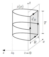
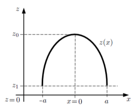
Figure III.1: (a) The rectangular loop is located at $z=0$. The corresponding world sheet $z(x)$ lives in the bulk. For $T\to\infty$, the world sheet parametrization $z(x)$ is $t$ independent. (b) A worldsheet section for fixed $t$. In this case the contour is located at a value $z_{1}$. This value can be sent to zero after substraction.

As described in the second figure, the loop is located at a value $z_{1}$ of the coordinate orthogonal to the border, in addition the corresponding minimal surface is required to be regular at the origin. Therefore the boundary conditions for the minimal surface are,

$$z(a)=z_{1}\;,z^{\prime}(0)=0\,\textrm{.}$$

The potential between static quarks can be obtained from the NG action as follows,

$$V_{\bar{q}q}(R)=\underset{T\rightarrow+\infty}{\mathrm{lim}}\frac{S_{NG}}{T}=\frac{1}{\pi\alpha^{\prime}}\int_{0}^{a}dx\,\mathrm{e}^{2A(x)}\sqrt{1+z^{\prime}(x)^{2}}\,\mathrm{,}$$ (III.2)

where $R=2a$ is the interquark separation.

III.1 Hamilton-Jacobi approach

With the boundary conditions mentioned above, the on-shell NG action is a function of the interquark separarion $a$ and $z_{1}$, the location of the loop, i.e.,

$$S_{NG}=S_{NG}(a,z_{1})$$

the corresponding Hamilton-Jacobi equation is given by,

$$\frac{\partial S_{NG}(a,z_{1})}{\partial a}+H\left(z_{1},\frac{\partial S_{NG}(a,z_{1})}{\partial z_{1}},a\right)=0\,\mathrm{,}$$

where $H=H(z,p,x)$ is the Hamiltonian, $p$ the canonical conjugate momenta to $z$ and $x$ the coordinate along the spatial dimension of the loop. To make the calculations easier, it is helpfull to neglect the multiplicative factor $\frac{T}{\pi\alpha^{\prime}}$ in III.1 and reintroduce it in the final expression. Standard methods lead to,

$$H(z,p,x) = p\,z^{\prime}(z,p,x)-L(z,z^{\prime}(z,p,x),x)$$ (III.3)

$$= -\frac{\mathrm{e}^{2A(z)}}{\sqrt{1+z^{{}^{\prime}2}}}=-\sqrt{\mathrm{e}^{4A(z)}-p^{2}}\,\mathrm{,}$$

leading to the following form of the HJ equation,

$$\frac{\partial S_{NG}(a,z_{1})}{\partial a}-\sqrt{\mathrm{e}^{4A(z_{1})}-\left[\frac{\partial S_{NG}(a,z_{1})}{\partial z_{1}}\right]^{2}}=0\,\textrm{.}$$ (III.4)

In this case, since the lagrangian does not depend on the coordinate $x$, the Hamiltonian is a constant of motion $E$, thus,

$$\frac{\partial S_{NG}(a,z_{1})}{\partial a}=\sqrt{\mathrm{e}^{4A(z_{1})}-\left[\frac{\partial S_{NG}(a,z_{1})}{\partial z_{1}}\right]^{2}}=-E$$

and the value of $E$ can be obtained from (III.3) as follows,

$$E=-\frac{\mathrm{e}^{2A(z)}}{\sqrt{1+z^{{}^{\prime}2}}}=-\mathrm{e}^{2A(z_{0})}$$

where $z_{0}$ is the maximum value of the coordinate $z$ attained by the minimal surface, which is therefore such that,

$$z_{0}=z(0)\>,\,z^{\prime}(0)=0\,\textrm{.}$$

An expression for $z_{0}$ as a fucntion of $a$ and $z_{1}$ can be obtained by means of,

$$a = \int_{0}^{a}dx=\int_{z(0)}^{z(a)}\frac{dx}{dz}\,dz$$ (III.5)

$$= \int_{z_{0}}^{z_{1}}\frac{1}{z^{\prime}}\,dz=\int_{z_{1}}^{z_{0}}\frac{\mathrm{e}^{2A(z_{0})}}{\sqrt{\mathrm{e}^{4A(z)}-\mathrm{e}^{4A(z_{0})}}}\,dz\,\textrm{.}$$ (III.6)

Having a constant of motion, a solution by separation of variables is possible,

$$S_{NG}(a,z_{1})=A(a)+Z(z_{1})$$

replacing in (III.4) gives,

$$A^{\prime}(a) = -E$$

$$Z^{\prime}(z_{1}) = \pm\sqrt{\mathrm{e}^{4A(z_{1})}-E^{2}}\,.$$

The general solution to these equations is,

$$A(a) = =-E\cdot a+A_{0}$$

$$Z(z_{1}) = -\int_{z_{inf}}^{z_{1}}\sqrt{\mathrm{e}^{4A(z)}-E^{2}}\,dz\,$$

where the integration constants $A_{0}$ and $z_{inf}$, has to be determined by choosing adequate boundary conditions. The followign boundary condition is adopted,

$$\lim_{a\to 0}S_{NG}(a,z_{1})=0\;\;,\,\forall\,z_{1}$$ (III.7)

this condition is satisfied by the following solution,

$$A(a) = =-E\cdot a$$

$$Z(z_{1}) = -\int_{z_{0}}^{z_{1}}\sqrt{\mathrm{e}^{4A(z)}-E^{2}}\,dz$$

Noting that $\lim_{a\to 0}z_{0}=z_{1}$, shows that the required boundary condition (III.7) is fullfilled.

Replacing $S_{NG}(a,z_{1})$ in (III.2), the interquark potential is given by,

$$V_{\bar{q}q}(R) = \frac{1}{2\pi\alpha^{\prime}}\bigg{[}R\,\mathrm{e}^{2A(z_{0})}+2\int_{z_{1}}^{z_{0}}\sqrt{\mathrm{e}^{4A(z)}-\mathrm{e}^{4A(z_{0})}}\,dz\bigg{]}\,,$$ (III.8)

which coincide with the results in kinar-sonnenschein:1998 . In order to express this potential in terms of $a$ and $z_{1}$, equation (III.5) can be employed to obtain $z_{0}$ as a function of is $a$ and $z_{1}$. In the AdS case $A(z)=-\ln\left(\frac{z}{L}\right)$, the integrals appearing in (III.5) and (III.8) are elliptic and can be evaluated to give expressions in terms of the hypergeometric function. In the general case, near the border, i.e. for $z_{1}\to 0$, the integrals can be evaluated up to terms proportional to positive powers of $z_{1}$, leading to,

$$V_{\bar{q}q}(R) = \frac{L^{2}}{2\pi\alpha^{\prime}}\bigg{[}\frac{R}{z_{0}^{2}}+\frac{\sqrt{\pi}\,\Gamma(-\frac{1}{4})}{4\,z_{0}\,\Gamma(\frac{5}{4})}+\frac{2}{z_{1}}\bigg{]}+\mathcal{O}(z_{1}^{3})$$

$$a = \frac{\sqrt{\pi}\,z_{0}\,\Gamma(\frac{3}{4})}{\Gamma(\frac{1}{4})}+\mathcal{O}(z_{1}^{3})\,\mathrm{.}$$ (III.9)

which clearly shows that there is a divergence for $z_{1}\to 0$. This happens also in the non-AdS case and is related to the divergence of the metric near the border. A substraction procedure should be employed to obtain a finite value. This substraction will be discussed in section 5.

IV Circular loop

The surface contoured by the circular loop is described by the following embedding,

$$x^{1} = 0$$

$$x^{\sigma} = 0\hskip 56.9055pt\forall k\neq\mu,\nu$$

$$x^{\mu} = r\,\mathrm{cos}(\varphi)$$

$$x^{\nu} = r\,\mathrm{sin}(\varphi)$$

$$x^{5} = z=z(r)\,\;\;,0\leq\varphi\leq 2\pi\;,0\leq r\leq a\mathrm{,}$$

it should be noted that the coordiante $z$ has been taken to depend only on $r$, due to the rotational symmetry of the countour and the metric. The corresponding geometrical setting is shown in Figure 4.1.

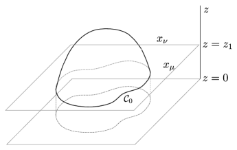
Figure IV.1: A loop located at $z=z_{1}$, and the corresponding world sheet.

The induced metric,

$$g_{ab}=G_{\mu\nu}\partial_{a}x^{\mu}\partial_{b}x^{\nu}\quad(a,b=\varphi,r)$$

and its determinant are given by,

$$g_{ab}=\begin{pmatrix}\left[1+z^{\prime}(r)^{2}\right]\mathrm{e}^{2A(z)}&0\\ 0&r^{2}\mathrm{e}^{2A(z)}\end{pmatrix}\;\;\;,\;\;\;\mathrm{det}(g_{ab})=r^{2}\,\left[1+z^{\prime}(r)^{2}\right]\mathrm{e}^{4A(z)}\,,$$

which leads to the following expression for the corresponding NG action,

$$S_{NG}=\frac{1}{\alpha^{\prime}}\int_{0}^{a}dr\,r\,\mathrm{e}^{2A(z)}\sqrt{1+z^{\prime}(r)^{2}}\,,$$ (IV.1)

where the $\varphi$ integration has been done, cancelling the $2\pi$ factor in (II.4). It is worth noting that this Lagrangian depends on the integration variable, and therefore the Hamiltonian is not a constant of motion in this case. The Euler-Lagrange equations of motion arising from this action are,

$$r\frac{z^{\prime\prime}(r)}{1+z^{\prime}(r)^{2}}+z^{\prime}(r)-2rA^{\prime}(z)=0$$ (IV.2)

the boundary conditions to be considered are,

$$z(a)=z_{1}\;,\,z^{\prime}(0)=0$$ (IV.3)

which correspond to a smooth surface contoured by a circular loop of radius $a$ located at the value $z_{1}$ of the coordinate $z$ ortogonal to the border. For the AdS case $A(z)=-\mathrm{ln}(\frac{z}{L})$, the solution to (IV.2) with the boundary conditions (IV.3) is,

$$z=\sqrt{a^{2}+z_{1}^{2}-r^{2}}\hskip 11.38109pt,0\leq r\leq a\,\mathrm{.}$$ (IV.4)

IV.1 Hamilton-Jacobi approach

In this case, the NG action is a function of the radius $a$ and the location $z_{1}$ of the circular loop. The momentum canonically conjugate to $z$ and the Hamiltonian appearing in the HJ equation are given by,

$$p(z,z^{\prime},r):=\frac{\partial L(z,z^{\prime},r)}{\partial z^{\prime}}=\frac{1}{\alpha^{\prime}}\frac{r\,z^{\prime}\,\mathrm{e}^{2A(z)}}{\sqrt{1+z^{{}^{\prime}2}}}\Rightarrow z^{\prime}(z,p,a)=\pm\frac{\alpha^{\prime}\,p}{\sqrt{r^{2}\mathrm{e}^{4A(z)}-\alpha^{\prime 2}\,p^{2}}}\,\mathrm{.}$$

$$H(z,p,r) = p\,z^{\prime}(z,p,r)-L(z,z^{\prime}(z,p,r),r)\vspace{3mm}$$ (IV.5)

$$= -\frac{p}{z^{\prime}(z,p,r)}=\mp\frac{1}{\alpha^{\prime}}\sqrt{r^{2}\,\mathrm{e}^{4A(z)}-\alpha^{\prime 2}p^{2}}\,.$$

Replacing in the HJ equation,

$$\frac{\partial S_{NG}(a,z_{1})}{\partial a}+H\left(z_{1},\frac{\partial S_{NG}(a,z_{1})}{\partial z_{1}},a\right)=0\,\mathrm{,}$$

leads to,

$$\frac{\partial S_{NG}(a,z_{1})}{\partial a}\mp\frac{1}{\alpha^{\prime}}\sqrt{a^{2}\,\mathrm{e}^{4A(z_{1})}-\alpha^{\prime 2}\left[\frac{\partial S_{NG}(a,z_{1})}{\partial z_{1}}\right]^{2}}=0\,\mathrm{,}$$ (IV.6)

which implies,

$$\left[\frac{\partial S_{NG}(a,z_{1})}{\partial a}\right]^{2}+\left[\frac{\partial S_{NG}(a,z_{1})}{\partial z_{1}}\right]^{2}=\frac{1}{\alpha^{\prime 2}}a^{2}\,\mathrm{e}^{4A(z_{1})}\,\mathrm{.}$$ (IV.7)

In the AdS case this equation is,

$$\left[\frac{\partial S_{NG}(a,z_{1})}{\partial a}\right]^{2}+\left[\frac{\partial S_{NG}(a,z_{1})}{\partial z_{1}}\right]^{2}=\frac{L^{4}}{\alpha^{\prime 2}}\frac{a^{2}}{z_{1}^{4}}\,\mathrm{,}$$

whose solution with the boundary condition,

$$\underset{a\rightarrow 0^{+}}{\mathrm{lim}}S_{NG}(a,z_{1})\,\equiv 0\quad(z_{1}=\mathrm{cte)}\>\mathrm{,}$$ (IV.8)

is,

$$S_{NG}^{AdS}(a,z_{1})=\frac{L^{2}}{\alpha^{\prime}}\left[\sqrt{1+\frac{a^{2}}{z_{1}^{2}}}-1\right]\,\mathrm{.}$$ (IV.9)

which coincides with what is obtained by replacing the solution (IV.4) in the NG action (IV.1).

IV.2 Expansion in powers of the radius $a$

An expansion of the on-shell NG action for the circular loop in powers of $a$, allows to obtain information about the gluon condensates in the dual gauge theory Shifman:1980ui Andreev:2007vn Quevedo:2013iya . It is not totally straightfoward to perform such an expansion. This can be seem from the result (IV.9) for the on-shell NG action in the AdS case. The series expansion of $S_{NG}^{AdS}(a,z_{1})$ in powers of $a$ is given by,

$$\frac{\alpha^{\prime}}{L^{2}}\,S_{NG}^{AdS}(a,z_{1})=\frac{a^{2}}{2z_{1}^{2}}-\frac{a^{4}}{8z_{1}^{4}}+\frac{a^{6}}{16z_{1}^{6}}+\mathcal{O}(a^{7})$$ (IV.10)

which is convergent for $\frac{a}{z_{1}}<1$. Therefore such an expansion is not suited to reproduce the behaviour of $S_{NG}^{AdS}(a,z_{1})$ for $z_{1}\to 0$ and $a$ fixed. Indeed, (IV.9) shows that,

$$\frac{\alpha^{\prime}}{L^{2}}\,S_{NG}^{AdS}(a,z_{1})\overset{{}_{z_{1}\ll 1}}{=}\frac{a}{z_{1}}$$ (IV.11)

In this respect it is convenient to consider the NG action in terms of the variables $w_{1}=\frac{z_{1}}{a}$ and $a$ instead of $z_{1}$ and $a$. Doing this for the AdS case gives,

$$\frac{\alpha^{\prime}}{L^{2}}\,S_{NG}^{AdS}(a,w_{1}a)=\frac{\sqrt{1+w_{1}^{2}}}{w_{1}}-1\>\mathrm{,}$$

whose Laurent expansion for $w_{1}\ll 1$ reproduces the divergence term $1/w_{1}$ in (IV.11), this is not the case for the expansion (IV.10).

Defining the action $S(a,w_{1})$ by,

$$S(a,w_{1})=S_{NG}(a,w_{1}a)$$

and taking into account that,

$$\frac{\partial S_{NG}(a,z_{1})}{\partial a} = \frac{\partial S(a,w_{1})}{\partial a}-\frac{w_{1}}{a}\,\frac{\partial S(a,w_{1})}{\partial w_{1}}$$

$$\frac{\partial S_{NG}(a,z_{1})}{\partial z_{1}} = \frac{1}{a}\,\frac{\partial S(a,w_{1})}{\partial w_{1}}\,\mathrm{,}$$

the HJ equation is rewritten as follows,

$$a^{2}\,\left[\frac{\partial S(a,w_{1})}{\partial a}\right]^{2}+\left(1+w_{1}^{2}\right)\left[\frac{\partial S(a,w_{1})}{\partial w_{1}}\right]^{2}$$

$$-2\,w_{1}\,a\,\frac{\partial S(a,w_{1})}{\partial a}\,\frac{\partial S(a,w_{1})}{\partial w_{1}} = \frac{1}{\alpha^{\prime 2}}\,a^{4}\,\mathrm{e}^{4A(w_{1}\cdot a)}\,\mathrm{,}$$ (IV.12)

the boundary condition (IV.8) is now,

$$0=\underset{a\rightarrow 0^{+}}{\mathrm{lim}}S_{NG}\left(a,z_{1}\right)=\begin{split}\underset{a\rightarrow 0^{+}}{\mathrm{lim}}S\left(a,\frac{z_{1}}{a}\right)\end{split} \quad(z_{1}=\mathrm{cst.)\>\mathrm{.}}$$ (IV.13)

Next the following power series expansion is considered,

$$S\left(a,w_{1}\right) = \frac{L^{2}}{\alpha^{\prime}}\,\sum_{n=0}^{\infty}s_{2n}\left(w_{1}\right)\,a{}^{2n}\>\mathrm{,}$$ (IV.14)

replacing this expansion in (IV.12) leads to,

$$\sum_{n=0}^{\infty}\left(\sum_{k=0}^{n}4(k+1)(n-k+1)\;s_{2(k+1)}(w_{1})\;s_{2(n-k+1)}(w_{1})\right)\,a^{2n+4}-$$

$$2\,w_{1}\,\sum_{n=0}^{\infty}\left(\sum_{k=0}^{n}2(k+1)\;s_{2(k+1)}(w_{1})\;s^{\prime}_{2(n-k)}(w_{1})\right)a^{2n+2}+$$

$$\left(1+w_{1}^{2}\right)\sum_{n=0}^{\infty}\left(\sum_{k=0}^{n}s^{\prime}_{2k}(w_{1})\;s^{\prime}_{2(n-k)}(w_{1})\right)\,a^{2n}-\sum_{n=0}^{\infty}\beta_{2n}\,w_{1}^{2n-4}\,a^{2n} = 0\,,$$ (IV.15)

where $\beta_{m}$ are the power series expansion coefficients of $\mathrm{e}^{4A(w_{1}a)}$, i.e.,

$$\mathrm{e}^{4A(w_{1}a)}=\frac{L^{4}}{\left(w_{1}a\right)^{4}}\,\mathrm{e}^{4f(w_{1}a)}=\frac{L^{4}}{\left(w_{1}a\right)^{4}}\,\sum_{n=0}^{\infty}\beta_{2n}\left(w_{1}a\right)^{2n}\,,$$

these coefficients can be written as polynomials in the $\alpha$ coefficients appearing in (II.3). Equating to zero the coefficient of $a^{n}$ in the l.h.s. of (IV.15), leads to,

$$2\left(1+w_{1}^{2}\right)\,s^{\prime}_{0}(w_{1})\,s^{\prime}_{2n}(w_{1})\,-4n\,w_{1\,}s^{\prime}_{0}(w_{1})\,s_{2n}(w_{1})\,+$$

$$\sum_{k=1}^{n-1}\left\{\left(1+w_{1}^{2}\right)\,s^{\prime}_{2k}(w_{1})\,s^{\prime}{}_{2(n-k)}(w_{1})\,+4k\left(n-k\right)\,s{}_{2k}(w_{1})\,s{}_{2(n-k)}(w_{1})\right.$$ (IV.16)

$$\left.-4w_{1}\,k\,s{}_{2k}(w_{1})\,s^{\prime}{}_{2(n-k)}(w_{1})\right\}-\beta_{2n}\,w_{1}^{2n-4} = 0\,,$$

valid for $n=0,1,2,\cdots$. The boundary condition (IV.13) leads to,

$$\underset{a\rightarrow 0^{+}}{\mathrm{lim}}S\left(a,z_{1}/a\right)=0\,\Longleftrightarrow\underset{a\rightarrow 0^{+}}{\mathrm{lim}}s_{2n}\left(z_{1}/a\right)\cdot a^{2n}=0\;\;\forall\,n,\,z_{1}=\textrm{cst}.$$ (IV.17)

For a given $n$, equation (IV.16) involves the functions $s_{2k}(w_{1})$ and $s^{\prime}_{2k}(w_{1})$ for $0\leq k\leq n$. Therefore starting with $n=0$, the resulting equation only involves $s_{0}(w_{1})$ and $s^{\prime}_{0}(w_{1})$, solving for them they can be replaced in the equation for $n=1$, to get $s_{2}(w_{1})$ and $s^{\prime}_{2}(w_{1})$ and so on. The equation for $n=0$ and its solution satisfying the boundary condition (IV.17) are,

$$[s^{\prime}_{0}(w_{1})]^{2}=\frac{1}{w_{1}^{4}\left(1+w_{1}^{2}\right)}\>\implies\>s{}_{0}(w_{1})=+\left(\frac{\sqrt{1+w_{1}^{2}}}{w_{1}}-1\right)\>\mathrm{,}$$ (IV.18)

where the sign in the second equation has been choosen so as to get a positive area for non-vanishing radius. For the cases with $n=1,2,\cdots$ the differential equations to be considered are of the form,

$$A^{(2n)}(w_{1})\,s^{\prime}_{2n}(w_{1})\,+B^{(2n)}(w_{1})\,s_{2n}(w_{1})\,+\,C^{(2n)}(w_{1})=0\,\textrm{,}$$ (IV.19)

the general solution to this equation is,

$$s_{2n}(w_{1}) = c^{(2n)}\,\mathrm{e}^{F(w_{1})}-\mathrm{e}^{F(w_{1})}\,\int_{0}^{w_{1}}\mathrm{e}^{-F(x)}\,\frac{C^{(2n)}(x)}{A^{(2n)}(x)}\,\mathrm{d}x\,\textrm{,}$$

$$F(w_{1}) = -\int_{0}^{w_{1}}\frac{B^{(2n)}(x)}{A^{(2n)}(x)}\,\mathrm{d}x\,\textrm{,}$$ (IV.20)

where $c^{(2n)}$ is a constant to be determined using the boundary condition (IV.17). Eq. (IV.16) implies that,

$$\frac{B^{(2n)}(x)}{A^{(2n)}(x)} =-2n \frac{w_{1}}{1+w_{1}^{2}}\quad\Longrightarrow\quad F(w_{1})=\mathrm{ln}\left[\left(1+w_{1}^{2}\right)^{n}\right]\,\textrm{,}$$

replacing in (IV.20) leads to,

$$s_{2n}(w_{1}) = c^{(2n)}\,\left(1+w_{1}^{2}\right)^{n}+\frac{1}{2}\,\left(1+w_{1}^{2}\right)^{n}\,\int_{0}^{w_{1}}\frac{x^{2}}{\left(1+x^{2}\right)^{n+\frac{1}{2}}}\,C^{(2n)}(x)\,\mathrm{d}x\,\textrm{,}$$ (IV.21)

where the following equalities were employed $A^{(2n)}(x)=2\left(1+x^{2}\right)\,s^{\prime}_{0}(x)=-\frac{2\sqrt{1+x^{2}}}{x^{2}}$. Inposing the boundary condition (IV.17) leads to,

$$c^{(2n)}=-\frac{1}{2}\int_{0}^{+\infty}\frac{x^{2}}{\left(1+x^{2}\right)^{n+\frac{1}{2}}}\,C^{(2n)}(x)\,\mathrm{d}x\,\textrm{,}$$

which replacing in (IV.21) gives,

$$s_{2n}(w_{1})=-\frac{1}{2}\,\big{(}1+w_{1}^{2}\big{)}\,\int_{w_{1}}^{+\infty}\frac{x^{2}}{\big{(}1+x^{2}\big{)}^{n+\frac{1}{2}}}\,C^{(2n)}(x)\,\mathrm{d}x\,\mathrm{,}$$ (IV.22)

the functions $C^{(2n)}$ appearing in this expression are obtained form (IV.16),

$$C^{(2n)}(x) = \sum_{k=1}^{n-1}\left\{\left(1+x{}^{2}\right)\,s^{\prime}_{2k}(x)\,s^{\prime}{}_{2(n-k)}(x)\,+\,4k\left(n-k\right)\,s{}_{2k}(x)\,s{}_{2(n-k)}(x)\right.$$ (IV.23)

$$\left.-4w_{1}\,k\,s{}_{2k}(x)\,s^{\prime}{}_{2(n-k)}(x)\right\}-\beta_{2n}\,x^{2n-4}\,\textrm{.}$$

for $n=0,1,2,3$ the results for $C^{(2n)}(x)$ and $s_{2n}(w_{1})$ are given in appendix A.

V Substraction

The substraction procedure employed is essentially the same as the one in Maldacena:1998im . It has been extended and applied to the non-AdS case in Quevedo:2013iya . The subtraction $S_{CT}$ to the NG action has a clear geometrical meaning which is illustrated in fig. V.1.

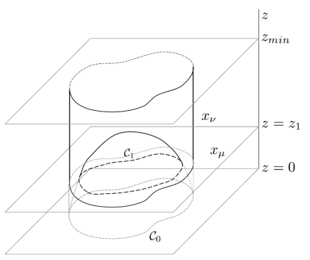
Figure V.1: Substraction scheme.

It corresponds to the area of a cylinder with section given by a countour such that the minimal area surrounded by this countour at $z=0$ intersects the plane $z=z_{1}$ with the original countour. For the case of confining warp factors the extension of this cylinder in the $z$ direction is regulated by an infrared cut-off $z_{IR}$. This is so because for those geometries the warp factor necesarily presents a minimum $z_{m}$ above which the warp factor growskinar-sonnenschein:1998 . In Quevedo:2013iya it is argued that a natural candidate for this infrared scale is the location of the warp factor minimum $z_{m}$. In any case as we shall see bellow the physical quantities to be calculated do not depend on this scale.

For the case of the rectangular loop $S_{CT}$ is given by,

$$S_{CT}=\frac{2}{2\pi\alpha^{\prime}}\int_{-\frac{T}{2}}^{\frac{T}{2}}dt\int_{z_{1}}^{z_{IR}}dz\,\mathrm{e}^{2A(z)}$$

for the AdS case this subtraction is,

$$S_{CT}^{AdS}=\frac{T}{\pi\alpha^{\prime}}\int_{z_{1}}^{z_{IR}}dz\,\frac{1}{z^{2}}=\frac{T}{\pi\alpha^{\prime}}\frac{1}{z_{1}}-\frac{T}{\pi\alpha^{\prime}}\frac{1}{z_{IR}}$$

which when substracted to $S_{NG}$ cancells the divergent term in (III.9).

For the circular loop the substracted on-shell NG action is given by,

$$S_{NG}^{sub}=S_{NG}-S_{CT}=S_{NG}-\frac{1}{2\pi\alpha^{\prime}}\,r_{0}(a,z_{1})\int_{z_{1}}^{z_{IR}}dz\,e^{2A(z)}\,,$$ (V.1)

For the AdS case the function $r_{0}(a,z_{1})$ is fixed by conformal invariance and is given by,

$$r_{0}^{AdS}(a,z_{1})=2\pi\sqrt{a^{2}+z_{1}^{2}}\,,$$ (V.2)

leading to,

$$S_{NG}^{sub,AdS}=-\frac{L^{2}}{\alpha^{\prime}}\,.$$ (V.3)

For the non-AdS case one could take $r_{0}(a,z_{1})$ to be the radius of a loop located at the boundary whose minimal surface would intersect the plane $z=z_{1}$ with a circle of radius $a$. However as explained in Quevedo:2013iya it is simpler to take the AdS expression given by (V.2), which presents no conflict with conformal invariance and leads to a finite substrated NG action even in the non-AdS case.

The choice of $z_{IR}$ does not affect the result for the condensates, since it only affects the coefficient of the perimeter in the expansion of the on-shell NG action in powers of the radius $a$.

V.1 Computing the subtraction

Fot the circular loop, in terms of $w_{1}=z_{1}/a$, the subtraction is given by,

$$S_{CT}=\frac{1}{\alpha^{\prime}}\,a\sqrt{1+w_{1}^{2}}\int_{w_{1}\cdot a}^{z_{IR}}\mathrm{e}^{2A\left(z\right)}\,\mathrm{d}z\,$$

the warp factor to be considered is given by (II.3), i.e.,

$$A(z)=-\log\left(\frac{z}{L}\right)+f(z)\;\;,\,f(z)=\sum_{k=1}\alpha_{2k}z^{2k}$$

thus,

$$\frac{\alpha^{\prime}}{L^{2}}\,S_{CT} = \frac{1}{L^{2}}\,a\sqrt{1+w_{1}^{2}}\int_{w_{1}\cdot a}^{z_{IR}}\mathrm{e}^{-2\log(\frac{z}{L})+2f(z)}\,\mathrm{d}z=\frac{1}{L^{2}}\,a\sqrt{1+w_{1}^{2}}\int_{w_{1}\cdot a}^{z_{IR}}\frac{L^{2}}{z^{2}}\mathrm{e}^{2f(z)}\,\mathrm{d}z$$

$$= a\sqrt{1+w_{1}^{2}}\int_{w_{1}\cdot a}^{z_{IR}}\frac{1}{z^{2}}\left(\mathrm{1+e}^{2f(z)}-1\right)\,\mathrm{d}z$$

$$= a\sqrt{1+w_{1}^{2}}\int_{w_{1}\cdot a}^{z_{IR}}\frac{1}{z^{2}}\,\mathrm{d}z\,+a\sqrt{1+w_{1}^{2}}\int_{w_{1}\cdot a}^{z_{IR}}\frac{\mathrm{e}^{2f(z)}-1}{z^{2}}\,\mathrm{d}z$$

$$= a\sqrt{1+w_{1}^{2}}\left.\left(-\frac{1}{z}\right)\right|_{w_{1}\cdot a}^{z_{IR}}\,+a\sqrt{1+w_{1}^{2}}\int_{w_{1}\cdot a}^{z_{IR}}\frac{\mathrm{e}^{2f(z)}-1}{z^{2}}\,\mathrm{d}z$$

$$= \frac{\sqrt{1+w_{1}^{2}}}{w_{1}}+a\sqrt{1+w_{1}^{2}}\left[-\frac{1}{z_{IR}}+\int_{w_{1}\cdot a}^{z_{IR}}\frac{\mathrm{e}^{2f(z)}-1}{z^{2}}\,\mathrm{d}z\right]\,,$$

the integrand in this last equation has no singularities in the integration region. Therefore the only singular term of this expression for $w_{1}\to 0$ is the first. This singular part coincides with the one in the AdS case. Indeed it is produced by the AdS term $-\log\left(\frac{z}{L}\right)$ of the warp factor. Thus the singular part of the counterterm is not affected by the addition of $f(z)$ to the warp factor.

V.2 The subtracted NG action

For the rectangular loop, the substracted NG action is given by,

$$S_{NG}^{sub} = S_{NG}-S_{CT}$$ (V.4)

$$= \frac{T}{2\pi\alpha^{\prime}}\bigg{[}R\,\mathrm{e}^{2A(z_{0})}+2\int_{z_{1}}^{z_{0}}\sqrt{\mathrm{e}^{4A(z)}-\mathrm{e}^{4A(z_{0})}}\,dz\bigg{]}-\frac{T}{\pi\alpha^{\prime}}\int_{z_{1}}^{z_{IR}}\mathrm{e}^{2A(z)}\,dz$$

$$= \frac{T}{2\pi\alpha^{\prime}}\bigg{[}R\,\mathrm{e}^{2A(z_{0})}+2\int_{z_{1}}^{z_{0}}\sqrt{\mathrm{e}^{4A(z)}-\mathrm{e}^{4A(z_{0})}}-\mathrm{e}^{2A(z)}\,dz\bigg{]}$$

$$-\frac{T}{\pi\alpha^{\prime}}\int_{z_{0}}^{z_{IR}}\mathrm{e}^{2A(z)}\,dz$$

The first integral is now finite even when $z_{1}\to 0$. This can be seen by noting that the integrand has no singularities and is well behaved when $z\to 0$, this is shown bellow,

$$\sqrt{\mathrm{e}^{4A(z)}-\mathrm{e}^{4A(z_{0})}}-\mathrm{e}^{2A(z)} = \sqrt{\mathrm{e}^{-4\log(\frac{z}{L})+4f(z)}-\mathrm{e}^{-4\log(\frac{z_{0}}{L})+4f(z_{0})}}-\mathrm{e}^{-2\log(\frac{z}{L})+2f(z)}$$

$$= \sqrt{\frac{L^{4}}{z^{4}}\mathrm{e}^{4f(z)}-\frac{L^{4}}{z_{0}^{4}}\mathrm{e}^{4f(z_{0})}}-\frac{L^{2}}{z^{2}}\mathrm{e}^{2f(z)}$$

$$= L^{2}\mathrm{e}^{2f(z)}\,\frac{\sqrt{1-\left(\frac{z}{z_{0}}\right)^{4}\mathrm{e}^{4\left[f(z_{0})-f(z)\right]}}-1}{z^{2}}$$

$$= L^{2}\mathrm{e}^{2f(z)}\,\frac{-\frac{1}{2}\left(\frac{z}{z_{0}}\right)^{4}\mathrm{e}^{4\left[f(z_{0})-f(z)\right]}+\mathcal{O}\left(\left(\frac{z}{z_{0}}\right)^{4}\mathrm{e}^{4\left[f(z_{0})-f(z)\right]}\right)^{2}}{z^{2}}$$

where in the last step the power series expansion of the square root was employed. The second integral in (V.4) is convergent and depends on the infrared cutoff $z_{IR}$. It is shown in kinar-sonnenschein:1998 that when the interquark separation is big ($R=2a\gg L$) the value of $z_{0}$ goes to $z_{m}$, the minimum of the warp factor, and consequently the interquark potential has a linear dependence on $R$,

$$V_{\bar{q}q}(R) = \sigma\,R+V_{0}\quad\textrm{if}\>R\gg L$$

where $\sigma=\frac{\mathrm{e}^{2A(z_{m})}}{2\pi\alpha^{{}^{\prime}}}$ is the quark-antiquark string tension. Warp factors such that $\mathrm{e}^{2A(z_{m})}\neq 0$ predict linear confinement as happens in QCD.

For the circular loop, according to (V.1), the subtracted NG action $S_{NG}^{sub}$ can be written as follows,

$$\frac{\alpha^{\prime}}{L^{2}}\,S_{NG}^{sub}(a,w_{1}) = \frac{\alpha^{\prime}}{L^{2}}\,S_{NG}(a,w_{1})-\frac{\alpha^{\prime}}{L^{2}}\,S_{CT}(a,w_{1})$$

$$= -1+\sum_{n=1}^{\infty}s_{2n}\left(w_{1}\right)\,a{}^{2n}-a\sqrt{1+w_{1}^{2}}\left[-\frac{1}{z_{IR}}+\int_{w_{1}\cdot a}^{z_{IR}}\frac{\mathrm{e}^{2f(z)}-1}{z^{2}}\,\mathrm{d}z\right]$$

$$\underset{w_{1}\rightarrow 0}{\longrightarrow} -1+\varPhi\left(z_{IR},\left\{\alpha_{2n}\right\}_{n=1}^{\infty}\right)\,a+\sum_{n=1}^{\infty}s_{2n}(0)\,a{}^{2n}\,\textrm{,}$$

where,

$$\varPhi\left(z_{IR},\left\{\alpha_{2n}\right\}_{n=1}^{\infty}\right) := \frac{1}{z_{IR}}-\int_{0}^{z_{IR}}\frac{\mathrm{e}^{2f(z)}-1}{z^{2}}\,\mathrm{d}z\,\textrm{.}$$

In the, limit $w_{1}\to 0$ with $a$ fixed the result for substracted on-shell NG action up to order $a^{6}$ is,

$$\frac{\alpha^{\prime}}{L^{2}}\,S_{NG}^{sub}\left(a\,,\,z_{1}=0\right) = -1+\varPhi\,a+2\alpha_{2}\,a^{2}+\left[\left(\frac{34}{3}-8\,\log(4)\right)\alpha_{2}^{2}+\frac{2}{3}\,\alpha_{4}\right]\,a^{4}\>$$

$$+\frac{2}{45}\big{[}\left(1774-2280\,\log\left(4\right)+720\,\log^{2}\left(4\right)\right)\alpha_{2}^{3}\vspace{3mm}$$

$$+\left(326-240\,\log\left(4\right)\right)\alpha_{2}\,\alpha_{4}+9\,\alpha_{6}\big{]}\,a^{6}+\ldots\mathrm{.}$$

Taking $\alpha_{2}=0$ (which corresponds to the absence of a dimension $2$ condensate in the border gauge theory) the calculation can be extended to higher orders. The result in this case up to order $a^{10}$ is,

$$\frac{\alpha^{\prime}}{L^{2}}\,S_{NG}^{sub}\left(a\,,\,z_{1}=0\right) = -1+\left.\varPhi\right|_{\alpha_{2}=0}\,a+\frac{2}{3}\,\alpha_{4}\,a^{4}\,+\frac{2}{5}\,\alpha_{6}\,a^{6}$$

$$+\left[\left(\frac{4222}{945}-\frac{32\,\log(4)}{9}\right)\alpha_{4}^{2}+\frac{2}{7}\alpha_{8}\right]\,a^{8}$$

$$+\left[\frac{4\left(2999-2520\,\log(4)\right)}{1575}\alpha_{4}\alpha_{6}+\frac{2}{9}\alpha_{10}\right]\,a^{10}+\ldots\mathrm{.}$$

VI Comparison with other computations

In this section the computations done above are compared with the analogous ones computed using the $\epsilon$-scheme. This is particularly relevant since, although the results coincide for the case of the rectangular loop, this is not the case for the circular loop. The result for the expansion coefficients $s_{2n}$ of the substracted NG action in powers of the radius $a$ in the limit $z_{1}\to 0$ for the case of the circular loop do not coincide between both schemes. The source of this coincidence and discrepancy are analysed below. In order to do this it is necesary to consider the process of regularization/substraction involved in the $\epsilon$-scheme. The $\epsilon$-regularization scheme is despicted in the following figure,

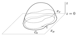
Figure VI.1: The $\epsilon$ regularization. .

For the non-conformal case this scheme is considered in Andreev:2007vn . It consists in locating the countour of the loop at the boundary $z=0$, obtaining the corresponding minimal surface and computing its area up to a value of the coordinate orthogonal to the border which is an amount $\epsilon$ less than the one of the original countour. Thus varying the diameter of the countour or the cut-off $\epsilon$ amounts to the same thing for the on-shell NG action. In addition, the boundary conditions are given at a value of $z$ that does not correspond to the location of the base of the surface whose area is calculated. In other words, the value of the $z$ coordinate corresponding to the location of the loop countour is not a variable and is fixed to zero. Therefore this scheme is not well suited for employing the HJ method. Nevertheless, the value of the on-shell NG action can be calculated by solving the equation of motion (IV.2) with boundary conditions,

$$z(a)=0\;,\,z^{\prime}(0)=0$$

and replacing in the NG action. Alternativedly, one can employ the solution to the equation of motion (IV.2) with the boundary conditions (IV.3) and take the limit $z_{1}\to 0$ in the integrand of the NG action. This last approach was employed in Quevedo:2013iya .

The substraction to be employed is the same as the one described in section V.

VI.1 The rectangular loop

The solution to the equations of motion for this case can be obtained by noting that the Hamiltonian corresponding to the Lagrangian appearing in (III.1) is a constant of motion $E$, given by,

$$E=-\frac{e^{2A}}{\sqrt{1+z^{\prime}(x)^{2}}}$$

where the ^′ indicates derivative respect to $x$. This leads to the following linear ordinary diferential equation,

$$z^{\prime}(x)=\sqrt{\frac{e^{4A}}{E^{2}}-1}$$

from which it is simple to obtain $x$ as a function of $z$,

$$x(z)=a-\int_{z_{1}}^{z}dz\frac{E}{\sqrt{e^{4A}-E^{2}}}$$ (VI.1)

this solution satisfies the boundary condition $x(z_{1})=a$, and therefore corresponds to a pair of static quarks located at $z=z_{1}$ and separated a distance $2a$. The relation between $z_{1}$, $z_{0}$, $E$ and $a$ can be obtained using that by definition $x(z_{0})=0$, leading to,

$$a=\int_{z_{1}}^{z_{0}}dz\frac{E}{\sqrt{e^{4A}-E^{2}}}$$ (VI.2)

In order to insert this solution in the Nambu-Goto action it is convenient to consider an alternative embedding of the same surface in the five dimensional space. In this embedding one considers $x$ as a function of $z$. It is given by,

$$x^{1} = t\hskip 42.67912pt,\;t\in\bigl{[}{\textstyle{\textstyle-\frac{T}{2},\frac{T}{2}}}\bigr{]}$$

$$x^{i} =x= x(z)\qquad\;,\;x\in[-a,a]$$

$$x^{k} = 0\hskip 42.67912pt,\,\forall k\neq i$$

$$x^{5} = z\,\mathrm{.}$$

the NG action is given in terms of this embedding by,

$$S_{NG}=\frac{1}{2\pi\alpha^{\prime}}\int_{-\frac{T}{2}}^{\frac{T}{2}}dt\int_{z_{1}}^{z_{0}}dz\,\mathrm{e}^{2A(z)}\sqrt{1+x^{\prime}(z)^{2}}$$ (VI.3)

where now the ^′ indicates derivative respect to $z$, $z_{1}$ is the location of the loop countour and $z_{0}$ the maximum value of $z$ attained by the minimal surface. Evaluation of the NG action in the solution of the equations of motion amounts to replace (VI.1) in (VI.3). The integrand in (VI.3) is independent of $z_{1}$, because $x^{\prime}(z)$ is independent of $z_{1}$ as implied by (VI.1). The lower integration limit is common to the HJ and the $\epsilon$-regularization. The upper limit of integration is to be determined as a function of $a$ and $z_{1}$ by means of (VI.2). For the $\epsilon$-regularization this amounts to take $z_{1}\to 0$ in (VI.2). The function $z_{0}(a,z_{1})$ just gives the maximum of the minimal surface, this function has no singularities for any value of $z_{1}\geq 0$. Therefore taking the limit $z_{1}\to 0$, before or after the integration makes no difference. Thus the result for the substracted NG action is the same for both schemes.

VI.2 Circular loop

The results for the expansion coefficients $s_{2n}$ of the NG action in powers of the radius $a$ for the case of the circular loop are shown in the table bellow. The first column corresponds to the results computed with HJ-scheme. The second column corresponds to the results computed in Quevedo:2013iya using the $\epsilon$-scheme . The first two rows in column $\epsilon$ also coincide with the results in Andreev:2007vn , which takes $\alpha_{n}=\delta_{n2}\alpha_{2}$. In the $\epsilon$-computation the loop is located at $z=0$.

$s_{2n}$	HJ	$\epsilon$
$s_{2}$	$2\alpha_{2}$	$\frac{10}{3}\alpha_{2}$
$s_{4}$	$\frac{2}{3}(17-24\log 2)\alpha_{2}^{2}+\frac{2}{3}\alpha_{4}$	$\frac{14}{9}(17-24\log 2)\alpha_{2}^{2}+\frac{14}{9}\alpha_{4}$
$s_{6}$	$\frac{2}{5}\alpha_{6}$	$\frac{3}{5}\alpha_{6}$
$s_{8}$	$\frac{2}{945}(2111-3360\log 2)\alpha_{4}^{2}+\frac{2}{7}\alpha_{8}$	$\frac{11}{5670}[(2111-3360\log 2)\alpha_{4}^{2}+270\alpha_{8}]$
$s_{10}$	$\frac{4}{1575}(2999-5040\log 2)\alpha_{4}\alpha_{6}+\frac{2}{9}\alpha_{10}$	$\frac{13}{4725}[(2999-5040\log 2)\alpha_{4}\alpha_{6}+175\alpha_{10}]$

Table 1: Results for the expansion coefficients of the NG action for the circular loop in powers of the radius $a$.

These two approaches where considered in Drukker:1999zq for the case of the supersymmetric conformal theory. They essentially differ in the regularization employed. In Drukker:1999zq it is shown that in the AdS case for smooth surfaces both regularizations lead to the same results, except in what respects to zig-zag symmetry. The HJ-regularization respects this symmetry but the $\epsilon$-regularization does not. Bellow, these regularizations are compared for the non-AdS case.

Clearly the results appearing in the two colums in table 1 are different. Bellow, it is shown that the two computations would reduce to a single one if an interchange of limits and integration would be valid, which is not the case.

The results for the $HJ$-regularization can be computed either by the HJ approach or solving the differential equation and replacing the solution in the NG action. Both methods lead to the same results. In the second approach there appear terms in the integrand that go to zero when $z_{1}\to 0$ but survive after integration. These terms are responsable for the discrepancy with the $\epsilon$-regularization which, as mentioned before, is equivalent to taking the limit $z_{1}\to 0$ in the integrand before performing the integral. In appendix B a concrete example is considered which shows how these terms arise for the case of the coefficient $s_{2}$.

The main difference between both approaches is that, in the HJ-regularization, boundary conditions for the minimal surface are taken at its border, i.e. where the base loop lies. In the $\epsilon$-regularization boundary conditions are taken at $z=0$ , which is not the location of the calculated area border. This implies that in this last case, the calculted area does not correspond to the area of a minimal surface, whose border lies at $z=0$, but to a fraction of it. In the limit $\epsilon\to 0$ the difference would vanish, however the divergence of the metric for $z\to 0$, gives a non vanishing contribution, which accounts for the difference between both results. In this respect it is worth noting, that such difference is not seen in the AdS case, simply because in that case conformal invariance requires the vanishing of the condensates.

VII Concluding remarks

In this work the HJ approach has been employed for the calculation of minimal areas on asymptotically AdS spaces. These calculations are relevant, from the holographic point of view, in obaining expectation values of Wilson loops in the gauge theory living at the border of these spaces. In this respect it is worth noting that,

• This approach directly calculates the minimal area without need to solve the equations of motion and replace the solution in the NG action. This makes the calculation more direct and in practice much simpler.

• In this approach variations of the on-shell classical action under changes in its boundary conditions are studied. The location of the loop countour is one of these conditions. Therefore the HJ-approach also leads to a natural regularization, which consists in moving the location of the countour out of the border.

Regarding the issue of regularization schemes it was shown that different schemes lead to different results. If one requires zig-zag symmetry to be respected then, as shown in Drukker:1999zq , the HJ scheme should be choosen. In this respect it is important to note that the HJ-scheme for any value of the regularization parameter $z_{1}$, computes the area of a minimal surface. This is not the case for the $\epsilon$-scheme.

Appendix A: The first terms in the expansion in powers of the radius.

$$C^{(2)}(x) = -\frac{\beta_{2}}{x^{2}}\,\textrm{,}$$

$$s_{2}(w_{1}) = -w_{1}\,\sqrt{1+w_{1}^{2}}\,\frac{\beta_{2}}{2}+\frac{\beta_{2}}{2}\,\left(1+w_{1}^{2}\right).$$

$$C^{(4)}(x) = \left(1+x^{2}\right)\,s^{\prime}_{2}(x)^{2}-4\,x\,s^{\prime}_{2}(x)\,s_{2}(x)+4\,s_{2}(x)^{2}-\beta_{4}\,\textrm{,}$$

$$s_{4}(w_{1}) = \frac{1}{24}\left\{4\beta_{4}+4\beta_{4}\left(2+w_{1}^{2}\right)w^{2}-4\beta_{4}\,w_{1}^{3}\,\sqrt{w_{1}^{2}+1}\right.$$

$$+3\beta_{2}^{2}\left[w_{1}^{2}\left(9w_{1}^{2}-9w_{1}\sqrt{w_{1}^{2}+1}+14\right)-8\sqrt{w_{1}^{2}+1}+5w_{1}\right]$$

$$\left.+12\beta_{2}^{2}\left(1+w_{1}^{2}\right)^{2}\left[2\,\arcsin(w_{1})-\log\left(1+w_{1}^{2}\right)-\log\left(4\right)\right]\right\}\,\textrm{.}$$

$$C^{(6)}(x) = 2\left(1+x^{2}\right)\,s^{\prime}_{2}(x)\,s^{\prime}_{4}(x)-8x\,s_{4}(x)\,s^{\prime}_{2}(x)-4x\,s{}_{2}(x)\,s^{\prime}_{4}(x)+16\,s{}_{2}(x)\,s{}_{4}(x)-\beta_{6}\,x^{2}\,\textrm{,}$$

$$s_{6}(w_{1}) = -\frac{1}{48}\left(1+w_{1}^{2}\right)^{3}\left\{-\frac{24}{5}\beta_{6}-24\beta_{2}^{3}\,\log^{2}(4)+3\beta_{2}^{3}\left[36\,\log(4)-73\right]+\frac{4}{3}\beta_{2}\beta_{4}\left[24\log(4)-59\right]\right.$$

$$-\frac{8\left(3\beta_{2}^{2}+\beta_{4}\right)\beta_{2}}{\left(1+w_{1}^{2}\right)^{2}}+\frac{204\beta_{2}^{3}+48\beta_{2}\beta_{4}}{1+w_{1}^{2}}-24\beta_{2}^{3}\,\log^{2}\left(1+w_{1}^{2}\right)-96\beta_{2}^{3}\,\log(2)\,\log\left(1+w_{1}^{2}\right)$$

$$+4\left(27\beta_{2}^{3}+8\beta_{2}\beta_{4}\right)\,\log\left(1+w_{1}^{2}\right)+\frac{192\beta_{2}^{3}\,w_{1}\,\arcsin(w_{1})}{\sqrt{1+w_{1}^{2}}}+\frac{96\beta_{2}^{3}\,\arcsin(w_{1})}{1+w_{1}^{2}}$$

$$-\frac{48\beta_{2}^{3}\,\log\left(4+4w_{1}^{2}\right)\left(1+2w_{1}\,\sqrt{1+w_{1}^{2}}-2\left(1+w_{1}^{2}\right)\arcsin(w_{1})\right)}{w^{2}+1}$$

$$-96\beta_{2}^{3}\,\arcsin^{2}(w_{1})-216\beta_{2}^{3}\,\arcsin(w_{1})-64\beta_{2}\beta_{4}\,\arcsin(w_{1})$$

$$\left.+w_{1}\,\frac{72\beta_{6}\,w_{1}^{4}+45\beta_{2}^{3}\left(73w_{1}^{4}+112w_{1}^{2}+40\right)+20\beta_{2}\beta_{4}\left(59w_{1}^{4}+104w_{1}^{2}+48\right)}{15\left(1+w_{1}^{2}\right)^{5/2}}\right\}\,\textrm{.}$$

Appendix B: The difference between the $z_{1}$-regularization and the $\epsilon$-regularization

In terms of the variables,

$$t=\sqrt{1+\left(\frac{z_{1}}{a}\right)^{2}-\left(\frac{r}{a}\right)^{2}}\;\;,\psi(t)=\left(\frac{z}{a}\right)^{2}$$

the NG action is,

$$S_{NG}=\frac{L^{2}}{\alpha^{\prime}}\int_{w_{1}}^{\sqrt{1+w_{1}^{2}}}\frac{e^{2(a^{2}\alpha_{2}\psi+a^{4}\alpha_{4}\psi^{2})}t\sqrt{4+\frac{\left(1+w_{1}^{2}-t^{2}\right)\psi^{\prime}(t)^{2}}{t^{2}\psi\left(t\right)}}}{2\psi\left(t\right)}dt\;.$$ (VII.1)

the solution to the equation of motion with the boundary conditions,

$$\psi(w_{1})=w_{1}^{2}\;\equiv(z(a)=z_{1})\;,\;\psi^{\prime}(\sqrt{1+w_{1}^{2}})=0\;,\equiv(z^{\prime}(0)=0)\text{ }$$

up to order $a^{2}$ is given by,

$$\psi(t) = t^{2}-4a^{2}\alpha_{2}\left(w_{1}^{2}+1\right)\left(\left(w_{1}^{2}+1\right)\log\left(-t^{2}+w_{1}^{2}+1\right)+\right.$$

$$\left.+(w_{1}-t)\left(-t+2\sqrt{w_{1}^{2}+1}-w_{1}\right)\right.$$

$$\left.+2\left(w_{1}^{2}+1\right)\tanh^{-1}\left(\frac{t}{\sqrt{w_{1}^{2}+1}}\right)-2\left(w_{1}^{2}+1\right)\sinh^{-1}(w_{1})\right)$$

replacing in (VII.1) gives the following expression for the integrand up to order $a^{2}$,

$$I(w_{1},t) = \frac{\sqrt{1+w_{1}^{2}}}{t^{2}}+a^{2}\frac{2\alpha_{2}\sqrt{w_{1}^{2}+1}}{t^{4}}\left(2t^{4}+4t^{2}w_{1}^{2}-2t^{2}w_{1}\sqrt{w_{1}^{2}+1}\right.$$

$$\left.-t^{2}w_{1}^{2}\log\left(-t^{2}+w_{1}^{2}+1\right)-t^{2}\log\left(-t^{2}+w_{1}^{2}+1\right)+6w_{1}^{2}\log\left(-t^{2}+w_{1}^{2}+1\right)\right.$$

$$\left.+3\log\left(-t^{2}+w_{1}^{2}+1\right)+2\left(w_{1}^{2}+1\right)\left(t^{2}-3\left(w_{1}^{2}+1\right)\right)\sinh^{-1}(w_{1})\right.$$

$$\left.-2\left(w_{1}^{2}+1\right)\left(t^{2}-3w_{1}^{2}-3\right)\tanh^{-1}\left(\frac{t}{\sqrt{w_{1}^{2}+1}}\right)+3w_{1}^{4}\log\left(-t^{2}+w_{1}^{2}+1\right)\right.$$

$$\left.+3t^{2}-6t\,w_{1}^{2}\sqrt{w_{1}^{2}+1}-6t\sqrt{w_{1}^{2}+1}-3w_{1}^{4}-3w_{1}^{2}+6w_{1}\sqrt{w_{1}^{2}+1}+6w_{1}^{3}\sqrt{w_{1}^{2}+1}\right)$$

the last term in this integrand is proportional to $w_{1}^{3}/t^{4}$, which vanish when $w_{1}\to 0$. However integrating and then taking the limit, they lead to a non-vanishing result,

$$\int_{w_{1}}^{\sqrt{1+w_{1}^{2}}}dt\;\frac{w_{1}^{3}}{t^{4}}=\left.-\frac{1}{3}\frac{w_{1}^{3}}{t^{3}}\right|_{w_{1}}^{\sqrt{1+w_{1}^{2}}}\stackrel{{{}_{w_{1}\to 0}}}{{=}}\frac{1}{3}\,\textrm{.}$$

References

• [1] G. ’t Hooft. A Planar Diagram Theory for Strong Interactions. Nucl.Phys., B72:461, 1974.
• [2] J. M. Maldacena. The Large N limit of superconformal field theories and supergravity. Adv.Theor.Math.Phys., 2:231–252, 1998.
• [3] E. Witten. Anti-de Sitter space and holography. Adv.Theor.Math.Phys., 2:253–291, 1998.
• [4] S.S. Gubser, I. R. Klebanov, and A. M. Polyakov. Gauge theory correlators from noncritical string theory. Phys.Lett., B428:105–114, 1998.
• [5] O. Aharony, S. S. Gubser, J. M. Maldacena, H. Ooguri, and Y. Oz. Large N field theories, string theory and gravity. Phys.Rept., 323:183–386, 2000.
• [6] S. S. Gubser. Dilaton driven confinement. 1999.
• [7] T. Sakai and S. Sugimoto. Low energy hadron physics in holographic QCD. Prog.Theor.Phys., 113:843–882, 2005.
• [8] L. Da Rold and A. Pomarol. Chiral symmetry breaking from five dimensional spaces. Nucl.Phys., B721:79–97, 2005.
• [9] J. Erlich, E. Katz, D. T. Son, and M. A. Stephanov. QCD and a holographic model of hadrons. Phys.Rev.Lett., 95:261602, 2005.
• [10] J. Polchinski and M. J. Strassler. The String dual of a confining four-dimensional gauge theory. 2000.
• [11] C. Csaki and M. Reece. Toward a systematic holographic QCD: A Braneless approach. JHEP, 0705:062, 2007.
• [12] J. M. Maldacena. Wilson loops in large N field theories. Phys.Rev.Lett., 80:4859–4862, 1998.
• [13] S. Rey and J. Yee. Macroscopic strings as heavy quarks in large N gauge theory and anti-de Sitter supergravity. Eur.Phys.J., C22:379–394, 2001.
• [14] Nadav Drukker, David J. Gross, and Hirosi Ooguri. Wilson loops and minimal surfaces. Phys.Rev., D60:125006, 1999.
• [15] R. Carcasses Quevedo, J.L. Goity, and R. Trinchero. QCD condensates and holographic Wilson loops for asymptotically AdS spaces. Phys.Rev., D89(3):036004, 2014.
• [16] U. Gursoy and E. Kiritsis. Exploring improved holographic theories for QCD: Part I. JHEP, 0802:032, 2008.
• [17] J. L. Goity and R. C. Trinchero. Holographic models and the QCD trace anomaly. Phys.Rev., D86:034033, 2012.
• [18] Y. Kinar, E. Schreiber, and J. Sonnenschein. Q anti-Q potential from strings in curved space-time: Classical results. Nucl.Phys., B566:103–125, 2000.
• [19] M. A. Shifman. Wilson Loop in Vacuum Fields. Nucl.Phys., B173:13, 1980.
• [20] O. Andreev and V. I. Zakharov. Gluon Condensate, Wilson Loops and Gauge/String Duality. Phys.Rev., D76:047705, 2007.