Origin of the 30 THz emission detected during the 2012 March 13 solar flare at 17:20 UT
Solar Physics

Abstract

Solar observations in the infrared domain can bring important clues on the response of the low solar atmosphere to primary energy released during flares. At present the infrared continuum has been detected at 30 THz (10 $\mu$m) in only a few flares. SOL2012-03-13 , which is one of these flares, has been presented and discussed in Kaufmann et al. (2013). No firm conclusions were drawn on the origin of the mid-infrared radiation. In this work we present a detailed multi-frequency analysis of the SOL2012-03-13 event, including observations at radio millimeter and sub–millimeter wavelengths, in hard X-rays (HXR), gamma-rays (GR), H$\alpha$, and white-light. HXR/GR spectral analysis shows that SOL2012-03-13 is a GR line flare and allows estimating the numbers of and energy contents in electrons, protons and $\alpha$ particles produced during the flare. The energy spectrum of the electrons producing the HXR/GR continuum is consistent with a broken power-law with an energy break at $\sim$ 800 keV. It is shown that the high-energy part (above $\sim$ 800 keV) of this distribution is responsible for the high-frequency radio emission ($>$ 20 GHz) detected during the flare. By comparing the 30 THz emission expected from semi-empirical and time-independent models of the quiet and flare atmospheres, we find that most ($\sim$80%) of the observed 30 THz radiation can be attributed to thermal free–free emission of an optically-thin source. Using the F2 flare atmospheric model (Machado et al., 1980) this thin source is found to be at temperatures T $\sim$ 8000 K and is located well above the minimum temperature region. We argue that the chromospheric heating, which results in 80 % of the 30 THz excess radiation, can be due to energy deposition by non-thermal flare accelerated electrons, protons and $\alpha$ particles. The remaining 20% of the 30 THz excess emission is found to be radiated from an optically-thick atmospheric layer at T $\sim$ 5000 K, below the temperature minimum region, where direct heating by non-thermal particles is insufficient to account for the observed infrared radiation.

1 Introduction

S-Intro Solar flare continuum observations from the mid-infrared domain (a few tens of THz) to the millimeter–sub-millimeter radio domain provide in principle unique diagnostics of energy transport processes from the flare energy release region to the chromosphere and of the most energetic flare accelerated particles (e.g. Trottet and Klein, 2013, and references therein). Since year 2000, radio observations at 212 and 405 GHz have been routinely obtained by the Solar Submillimeter Telescope (SST) and more recently high-cadence imaging observations of both the quiet Sun and flares have been obtained at 30 THz (Kaufmann et al., 2008, and references therein). The 2012 March 13 flare at $\sim$ 17:22 UT ( SOL2012-03-13) was the first flare observed at 30 THz (Kaufmann et al., 2013). Since then other flares detected at 30 THz have been reported in the literature (Kaufmann et al., 2015, and references therein). During SOL2012-03-13  the time evolution of the 30 THz impulsive emission was found to be similar to that of the radio (1-212 GHz), hard X-ray and white-light emission. The 30 THz emitting source was also co-spatial with a region of flare-enhanced white light continuum. No firm conclusion on the origin of the 30 THz infrared emission observed during SOL2012-03-13 was drawn by Kaufmann et al. (2013). Nevertheless, they suggested that it is consistent with heating of the flaring atmosphere below the temperature minimum region which cannot be due to direct heating by hard X-ray emitting electrons, at least within the classic thick-target model. On the other hand, theoretical work by Ohki and Hudson (1975) raised the possibility that the infrared continuum at wavelengths shorter than $\sim$ 20 $\mu$m may arise from an optically-thin source at temperatures in the range of 10⁴–10⁵ K. This latter possibility is in line with the results of time-dependent simulations of the chromospheric heating by electron beams performed by Kašparová et al. (2009a).

The main goal of this paper is to investigate what is the origin of the infrared continuum detected at 30 THz during SOL2012-03-13. For that we have performed a detailed analysis of multi-frequency observations including measurements in radio millimeter and sub millimeter wavelengths, hard X-ray (HXR) and gamma-ray (GR), H$\alpha$, and white-light (WL). The instrumentation used to collect these data is briefly described in Section S-Inst and an overview of the observations is presented in Section S-Over. Section S-xrgr is devoted to the analysis of HXR/GR spectra from which numbers and energy contents of electrons, protons and $\alpha$ particles accelerated during SOL2012-03-13 are estimated. In Section S-rad we discuss the relationship between HXR/GR and radio emitting electrons. The origin of the 30 THz emission is examined in Section S-30T by using semi-empirical time-independent models of both the quiet and flare chromosphere. In Section S-Resp we provide an estimate of the energy deposited by flare accelerated electrons, protons and $\alpha$ particles in the atmospheric layers which radiate the 30 THz emission and we examine if it can account for the energy radiated at 30 THz. The final Section summarizes the main conclusions.

2 Instrumentation

S-Inst

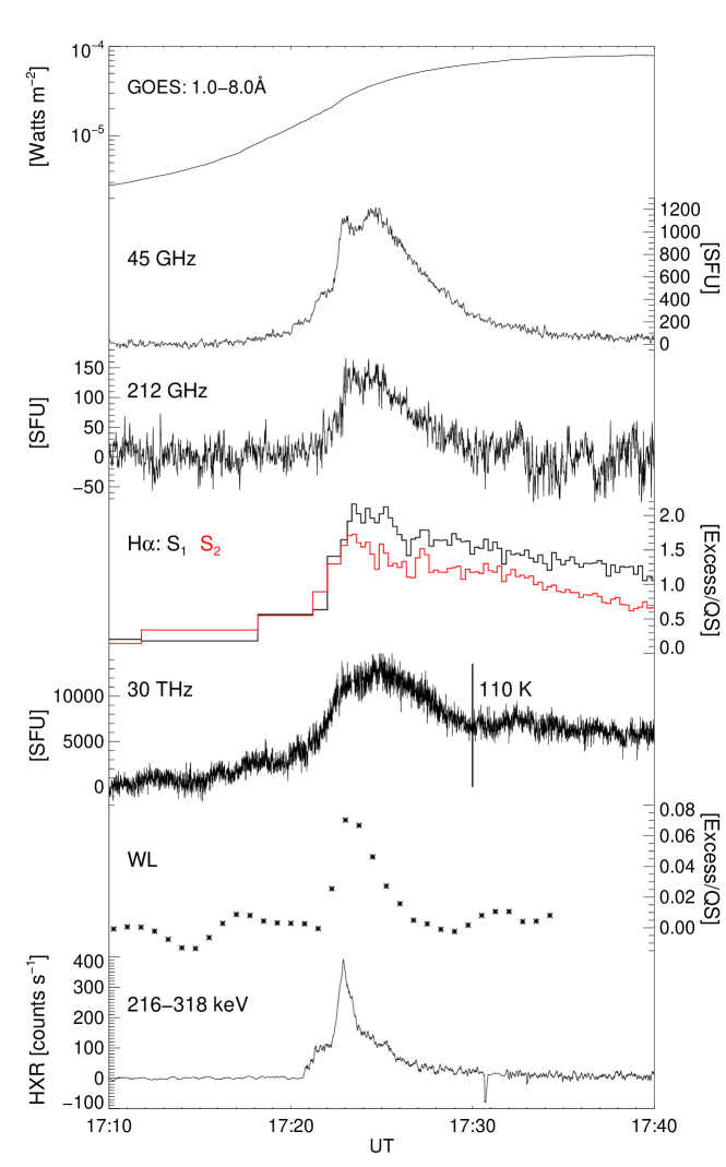
Figure 1.: Temporal evolution of the flare SOL2012-03-13 in various wavelength domains Fig˙over

Radio data at 45 GHz and 90 GHz were obtained by the radio polarimeters described in Valio et al. (2013). For the SOL2012-03-13 flare the uncertainty on flux densities is about 20%. Observations at 212 and 405 GHz have been provided by the SST. The atmospheric opacity was estimated to be 0.47 and 2.2 Nepers, at 212 and 405 GHz respectively. At 212 GHz the flux density accuracy is estimated to be 20%. At 405 GHz the 1 $\sigma$ detection threshold was $\sim$ 55 sfu, and no significant emission was detected.

In the HXR and GR domain, the SOL2012-03-13 flare has been detected by the Gamma-Ray Burst Monitor (GBM) on Fermi (Meegan et al., 2009). GBM is composed of twelve sodium-iodide (Na I) and two bismuth germanium oxide (BGO) detectors. In the present analysis we have used the most sunward Na I and BGO detectors. The Na I data consist in 128 energy channels covering the energy range 4 keV–2000 keV and the BGO data also consist of 128 energy channels but in the 113–50,000 keV range.

The 30 THz instrumental setup at El Leoncito is reported in Marcon et al. (2008) and Kaufmann et al. (2008). For the present solar flare the data calibration and the determination of the excess flux density relative to quiet Sun have been described in details in Kaufmann et al. (2013). The accuracy of flux density measurements has been estimated to be $\sim$ 25%. The diffraction limit of the instrument is $\sim$ 15^′′ and the source position uncertainty is $\sigma\sim$ 3^′′ as obtained from fitting of the 30 THz limb. The bandwidth of the instrument is $\sim$ 17 THz and in the following, we assume that the 30 THz emission does not depend on frequency within this bandwidth.

H$\alpha$ observations were obtained with the H-Alpha Solar Telescope for Argentina (HASTA; Bagalá et al., 1999). HASTA provides solar full disk images with a time resolution of 5 seconds in flare mode and a spatial resolution of 2^′′. Excess emission due to the flare has been normalized to the quiet Sun emission.

The above data set has been complemented by radio observations at 1.415, 2.695, 4.995 and 8.8 GHz from the Sagamore Hill-station of the US Air Force Radio Solar Telescope Network (RSTN) (Guidice, 1979). During SOL2012-03-13 there were no reliable 15.4 GHz measurements. We have also used WL images from the Helioseismic and Magnetic Imager (HMI; Scherrer et al., 2012) on board the Solar Dynamic Observatory (SDO) obtained every 45 s with a spatial resolution better than $\sim$ 1 ^′′  .

3 Observation overview

S-Over

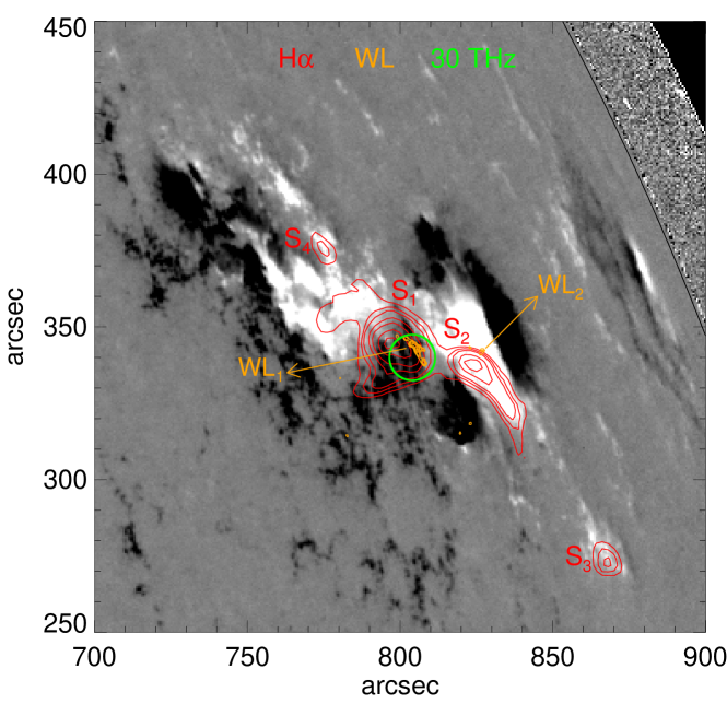
Figure 2.: Projections of H$\alpha$ (17:22:53 UT, red contours), WL (17:23:00 UT, yellow contours) and 30 THz (17:22:54 UT, green circle) sources on a SDO/HMI vector magnetogram obtained at 17:13:15 UTFig˙images

The flare SOL2012-03-13 occurred in NOAA active region AR 11429 located at N18W64 on 2012 March 13 at 22:00 UT. It was associated with a M7.9 soft X-ray (SXR) event detected by the Geostationary Operational Environmental Satellite (GOES) and with a H$\alpha$ flare of importance 1B. From top to bottom Fig. Fig_over displays the time profile of the SXR (1-8 Å) from GOES, radio (45 and 212 GHz), H$\alpha$, flare excess mid-infrared (30 THz), WL, and 216-318 keV HXR emissions detected during SOL2012-03-13. Except H$\alpha$ measurements, these observations have been presented in Kaufmann et al. (2013). The HXR light curve consists in an impulsive burst which started at $\sim$ 17:20:53 UT with a maximum at $\sim$ 17:22:54 UT and lasted for about ten minutes. This impulsive peak is seen from radio to optical wavelengths, i.e. from the corona down to the low chromosphere. At radio wavelengths, there are two peaks of apparently similar flux densities. There is a change of the decay slope of the HXR emission which corresponds to the second radio peak. The H$\alpha$, 30 THz and WL emissions show a broad peak which encompasses the two radio and HXR peaks. In addition to this impulsive phase, there is a long-lasting and slowly varying component seen at all wavelengths except in HXR and WL. For example at 45 GHz, although it is weak ($\sim$ 40-50 sfu), the gradual emission is still visible after 19:00 UT.

Figure Fig_images shows the projections of the H$\alpha$, WL and 30 THz sources, obtained around the maximum of the impulsive peak, on a vector magnetogram recorded by SDO/HMI at 17:13:15 UT. The flare enhanced H$\alpha$ emission arises from four sources (red contours) marked S₁, S₂, S₃ and S₄. S₁ and S₂ are close to the two WL emitting regions, WL₁ and WL₂, shown by yellow contours (see also Figures  3 and 10 in Kaufmann et al., 2013). The larger extents of WL₁ and WL₂ are respectively $\sim$ 10^′′ and 2^′′. The projections of WL₁ and WL₂ and S₁ and S₂ are located on opposite magnetic field polarities and are connected by a bright loop shown at 211 Å in Figure 5 of Kaufmann et al. (2013). At 30 THz only the source corresponding to S1 and to WL₁, the stronger WL emitting region, is detected within the sensitivity of the present setup of the 30 THz instrument. Since the 30 THz source is not resolved by the instrument, it is marked by a green circle whose diameter is the diffraction limit of the instrument (15^′′) in both directions. Figure Fig_images thus indicates that the 30 THz source and the WL barycenter emission, which is close to maximum of WL₁, are located close to each other. However, the uncertainty on the 30 THz source position (3 $\sigma\sim$ 9^′′) prevents to draw any conclusion on the relative height of both sources, for relative heights lower than few thousands of km. While the time profiles of S₁ and S₂ show a clear impulsive phase counterpart (see Figure Fig_over), the remote sources S₃ and S₄ only show a slowly varying emission that will not be considered in the following.

4 Electron and ion numbers and energy contents around the maximum of SOL2012-03-13

S-xrgr

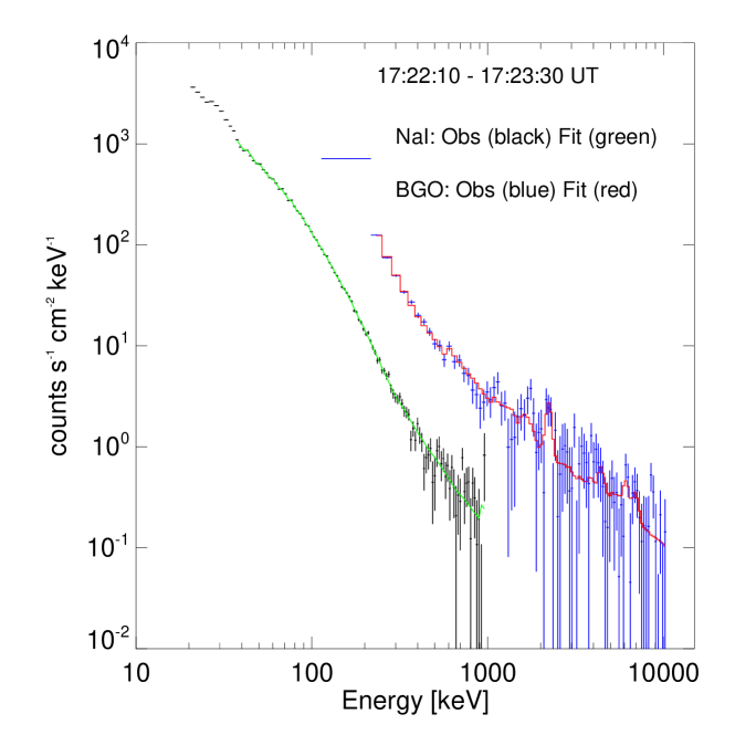
Figure 3.: HXR/GR spectrum around the maximum of SOL2012-03-13 obtained by combining BGO and Na I measurements of the GBM instrument on Fermi (error bars). The green and red curves show the model spectrun fitted to GBM observations (see text).Fig˙ferm

Figure Fig_ferm shows the mean excess count rate spectrum in the 20-10,000 keV range recorded by the most sunward NaI (black error bars) and the most sunward BGO (blue error bars) detectors, for a 80 s time interval around the peak of the HXR/GR emission. In the 36-1000 keV range, the observed NaI count rate spectrum is well represented by the expected count rate spectrum shown by the green line. This latter spectrum has been obtained by convolving a triple power-law photon spectrum with the NaI detector calibration matrix. The triple power-law spectrum represents the electron bremsstrahlung spectrum in the $\sim$ 35-1000 keV range. It is defined by the normalization factor at 50 keV, the power-law indices $\gamma_{1}$, $\gamma_{2}$ and $\gamma_{3}$ and the break energies Ebr₁ and Ebr₂ displayed in Table T1. In the 216-10,000 keV range, the BGO count rate spectrum is well represented by the expected count rate spectrum (red line) obtained for a photon spectrum which is the sum of a broken power-law, of the 2.2 MeV neutron capture line and of a template of narrow nuclear lines. We used the nuclear line template, included as standard within OSPEX (Schwartz et al., 2002), calculated for a flare at an heliocentric angle of $60^{\circ}$ by assuming a downward isotropic distribution of ions with a power-law energy distribution of index 4 and an $\alpha$/p ratio of 0.22. The broken power-law represents the electron bremsstrahlung spectrum in the 200-10,000 keV range. It is defined by the normalization factor at 50 keV, the power-law indices $\Gamma_{1}$ and $\Gamma_{2}$ and the break energy Ebra (see Table T2). For the fitting procedure we have used the OSPEX package of Solar Soft.

Table 1.: Parameters of the photon spectrum fitted to the NaI measurements in the 35-1000 keV T1

photons/s/cm2/keV	$\gamma_{1}$	Ebr1	$\gamma_{2}$	Ebr2	$\gamma_{3}$
at 50 keV		keV		keV
4.7 $\pm$ 1.5	3.3$\pm$ 0.2	94 $\pm$ 10	3.8 $\pm 0.2$	282 $\pm$ 20	2.4 $\pm$ 0.2

Table 2.: Parameters of the photon spectrum fitted to the BGO measurements in the 200-10,000 keV T2

photons/s/cm2/keV	$\Gamma_{1}$	Ebra	$\Gamma_{2}$	2.2 MeV line	narrow lines
at 50 keV		keV		photons/s	photons/s
5.7 $\pm$ 1.9	3.6 $\pm$ 0.2	388 $\pm$ 50	2.3 $\pm$ 0.2	0.054 $\pm$ 0.018	0.11 $\pm$ 0.04
electrons/s/keV	$\delta_{1}$	Ebre	$\delta_{2}$
at 50 keV		[keV]
$5.6\times 10^{33}$	4.7	800	3.5

Figure  Fig_ferm shows that: (i) the electron bremsstrahlung continuum extends up to at least 10,000 keV and (ii) there is clear 2.2 MeV line emission and weak narrow GR line emission indicating that $\sim$ 1-100 MeV protons and $\sim$ 1-100 MeV/nucleon ions have been accelerated during SOL2012-03-13. The photon fluxes derived from both Na I and BGO data agree well (within better than 25%) between 200-700 keV. However, because the responses of NaI and BGO detectors are quite different, a given incident photon spectrum will produce different count spectra in both types of detectors as shown in Figure  Fig_ferm. Above $\sim$ 400 keV, the 1-$\sigma$ uncertainty is smaller for BGO than for Na I. In the following we will only consider the photon spectrum derived from BGO data since we are interested in microwave emitting electrons and in GR line radiation. In order to derive the spectrum of electrons from this photon spectrum we further assume that this electron spectrum is also a broken power law. The electron spectrum is then derived by using an electron-to-thick-target bremsstrahlung code including both relativistic effects and electron-electron bremsstrahlung and by varying its parameters until a good agreement with the photon spectrum is reached. The obtained parameters are displayed in Table T2. The mean flux of $>$ 50 keV electrons between 17:22:10 and 17:23:30 UT is found to be F${}_{\rm{e}}(>50~{}\rm{keV})\sim 8\times 10^{34}$ electrons s^-1 corresponding to a mean energy flux $\Phi_{\rm{e}}(>50~{}\rm{keV})\sim 9\times 10^{27}$ ergs s^-1 . The nuclear line template is normalized so that an amplitude of 1 corresponds to 8.5946 $\times$ 10²⁹ protons with energies above 30 MeV. Here the amplitude of the nuclear line template is 0.11 $\pm$ 0.04 s^-1 (see Table T2). It is well documented that ions with energies down to almost 1 MeV/nucleon contribute to the GR line emission. For the assumed energy power-law index of 4 we then get mean proton and $\alpha$ fluxes at the top of the atmosphere: F${}_{\rm{p}}(>\rm{1~{}MeV})\sim 2.6\times 10^{33}$ protons s^-1, F${}_{\rm{\alpha}}(\rm{>1~{}MeV/nucl})\sim 5.6\times 10^{32}$ $\alpha$ s^-1. These correspond to energy fluxes of respectively $\Phi_{\rm{p}}(\rm{>1~{}MeV})=6.2\times 10^{27}$ ergs s^-1 and $\Phi_{\rm{\alpha}}(\rm{>1~{}MeV})\sim 5.4\times 10^{27}$ ergs s^-1. Since the uncertainty on the determination of photon fluxes is about 30%, the above values of particle and energy fluxes suffer from the same uncertainty. The broad GR line emission has not been taken into account to get the above estimates because, due to the poor statistics, the observed GR line spectrum is not well defined. Nevertheless, we have checked that the inclusion of broad lines lead to estimates of proton and $\alpha$ particle fluxes and energy fluxes that stay within the 30% uncertainty. It should be noted that $\Phi_{\rm{p}}\sim\Phi_{\rm{\alpha}}$ and that $\Phi_{\rm{e}}(>50~{}\rm{keV})\sim\Phi_{\rm{p}}(\rm{>1~{}MeV})+\Phi_{\rm{\alpha}}(\rm{>1~{}MeV})$.

5 Relationship between radio and HXR/GR emitting electrons during the impulsive phase

S-rad

Figure 4.: Radio spectrum: in both panels the vertical error bars show the radio spectrum observed in the 1-212 GHz frequency range around the maximum of the impulsive phase of SOL2012-03-13.̇ At 405 GHz the arrow indicates the upper limit of the flux density. The gyrosynchrotron spectra computed for $\rm{B=700~{}G}$ and $\rm{T_{trap}=2~{}s}$ , $\rm{E}_{\rm{max}}=10,000~{}\rm{keV}$ and $\rm{E}_{\rm{min}}=$ 30 keV (solid line), 400 keV (dotted line) and 800 keV (dashed line) are over plotted in the upper panel while results for $\rm{E}_{\rm{min}}=30~{}\rm{keV}$ and $\rm{E}_{\rm{max}}=$ 10,000 keV (solid line), 7,000 keV (dotted line) and 4,000 keV (dashed line) are over plotted in the lower panel (see text).Fig˙gyro

Figure Fig_gyro displays the averaged radio spectrum (vertical error bars) observed during the same time interval (17:22:10–17:23:30 UT) as the HXR/GR spectrum analyzed in Section S-xrgr. Its shape is reminiscent of a gyrosynchrotron spectrum with a turnover frequency somewhere between 10 and 30 GHz. It is generally admitted that the 1-200 GHz (cm-mm) radio emission and the HXR/GR continuum are both radiated by a closely related population of electrons accelerated in the corona (e.g. Bastian, Benz, and Gary, 1998; Pick and Vilmer, 2008). Briefly stated: (i) the gyrosynchrotron emission is radiated by the instantaneous population of electrons present in the coronal portion of magnetic loops connected to the acceleration region, while (ii) the HXR/GR bremsstrahlung continuum is produced by thick-target interactions of precipitating electrons at the chromospheric foot points of these loops. It is also well documented that for magnetic field of a few hundred Gauss the cm–mm emission is radiated by electrons with energies ranging from a few hundreds of keV to a few MeV (e.g. Ramaty, 1969; Pick, Klein, and Trottet, 1990; Ramaty et al., 1994). As a first approximation we thus assume that the instantaneous spectrum of radio emitting electrons is given by (e.g. Trottet et al., 1998): $\rm{N}_{\rm{R}}(\rm{E})\approx F_{\rm{X}}(\rm{E})~{}\rm{T}_{\rm{trap}}$ electrons keV^-1 where $\rm{T}_{\rm{trap}}$ is the time spent by the accelerated electrons in the cm–mm radio emitting region and F${}_{\rm{X}}(\rm{E)}$ is the electron flux spectrum displayed in Table T2. Without multi-frequency cm-mm imaging observations it is not possible to constrain radio source models with inhomogeneous magnetic field B and ambient density N_amb. In the following we thus compute the gyrosynchrotron emission produced by $\rm{N}_{\rm{R}}(\rm{E})$ in a radio emitting region of constant N_amb and uniform B. Such a simple model is not able to account for the $<$ 10 GHz optically-thick radio emission, but it allows one, in principle, to reasonably match the optically-thin part of the radio spectrum observed at 45, 90 and 212 GHz during the present flare. The gyrosynchrotron emission has then been computed for $\rm{B}=700$ G, $\rm{T}_{\rm{trap}}=2~{}s$ and N${}_{\rm{amb}}=5\times 10^{10}~{}\rm{cm}^{-3}$. The diameter and thickness of the radio source normal to and along the line of sight have been set to 14,000 and 2000 km respectively and the angle between B and the line of sight to $45^{\circ}$. The gyrosynchrotron code used is that by Ramaty (1969); Ramaty et al. (1994) adapted to take into account a broken power-law electron spectrum.

Figure Fig_gyro (upper panel) shows the results for an electron population with a high energy cutoff $\rm{E}_{\rm{max}}=10,000~{}\rm{keV}$ and different low-energy cutoffs $\rm{E}_{\rm{min}}=$ 30 keV (solid line), 400 keV (dotted line) and 800 keV (dashed line). In Fig. Fig_gyro (lower panel), $\rm{E}_{\rm{min}}=30~{}\rm{keV}$ and $\rm{E}_{\rm{max}}=$ 10,000 keV (solid line), 7,000 keV (dotted line) and 4,000 keV (dashed line). Figure Fig_gyro shows that the optically-thin part of the observed radio spectrum is emitted by electrons in the $\sim$ 800 to 7,000–10,000 keV energy range, that is above the break energy of the electron spectrum deduced from the HXR/GR photon spectrum. This is consistent with earlier findings (Trottet et al., 1998, 2000, 2008). B and T_trap, which fix the value of N_R, are not independent parameters in the data fitting process. Indeed, the same flux densities can be obtained for larger B and lower T_trap and vice versa. $\rm{B\sim 700~{}G}$ and $\rm{T_{trap}\sim 2~{}s}$ appears to be a reasonable set of values. On one hand, a substantial increase of B would lead to a too high turnover frequency. On the other hand, a decrease of B would imply an increase of $\rm{N_{R}}$. Since there is no physical reason to have E_min larger than a few tens of keV, a too low value of B would lead to an unreasonably high density of non-thermal electrons in the radio source compared to $\rm{N_{amb}}$.

6 Origin of the 30 THz emission

S-30T

In the following we assume that both the quiet and flare 30 THz emission is thermal emission from the chromosphere. The aim of this section is to search from which atmospheric layer(s) the 30 THz emission observed during the SOL2012-03-13 flare (see Section S-Over and Kaufmann et al., 2013) arises. As we do not know the actual flaring atmosphere, to achieve this, a first approach employs time-independent models of both the flaring and quiet lower atmospheres of the Sun. Such semi-empirical models are based on hydrostatic and statistical equilibria. For a given temperature structure the full non-LTE radiative transfer is solved numerically in order to obtain the synthetic flare spectrum. This synthetic spectrum is compared to observed spectral features (both lines and continuum) and the temperature structure is adjusted in order to get a good agreement with observations.

Tab_model Model h_max $\rm{\tau_{30}}$ $\Delta\rm{h}$ $\rm{T_{b30}}$ $\Delta$T_b30 $\Delta$S₃₀ [km] [km] [K] [K] [sfu] C7 180 1.1 130–270 4700 FLA 180 1.1 130–270 4900 200 1000 F1 180 1.4 140–300 5000 300 1500 F2 1070 0.2 960–1100 7100 2400 12,300

Table 3.: Height ( h_max), opacity ($\rm{\tau_{30}}$) at the maximum of CF₃₀. The altitudinal range $\Delta\rm{h}$ over which CF is larger than half of its maximum value. $\rm{T_{b30}}$ is the derived brightness temperature at 30 THz. $\Delta$T_b30 is the increase of $\rm{T_{b30}}$ with respect to C7 and $\Delta$S₃₀ is the excess flux density with respect to C7 for a 30 THz emitting source of 10^′′ diameter.

In order to compare expectations from flare models with quiet Sun conditions we have used the C7  model for the quiet solar atmosphere (Avrett and Loeser, 2008). The flare atmospheric models considered hereafter are: the FLA model constructed by Mauas, Machado, and Avrett (1990) to account for the WL continuum emission observed during the SOL1983-06-15 flare, and the F1 and F2 models representative of respectively weak and medium-size flares (Machado et al., 1980). We have restricted our analysis to these models because they are well documented in the literature and because SOL2012-03-13 is a medium size flare. We take their temperature height profiles as inputs and use the PAKAL radiative transfer code (De la Luz et al., 2010; De la Luz, Lara, and Raulin, 2011), which is similar to the PANDORA code used by Avrett and Loeser (2003), in order to: (i) compute the densities of electrons and of the most important ion species, including $\rm{H^{-}}$, as a function of height h and, (ii) determine the absorption coefficient $\rm{\kappa_{30}(h)}$ and the opacity $\rm{\tau_{30}(h)}$ for a 30 THz emitting region at a longitude of 60^∘. Following Heinzel and Avrett (2012), we then compute the contribution function $\rm{CF_{30}(h)}$ as a function of h, given by:

$$\mathrm{CF_{30}(h)}=\rm{\eta_{30}(h)e^{-\tau_{30}(h)}\ ,\quad\eta_{30}(h)=\kappa_{30}(h)B_{30}(T(h))\ },$$ (1)

where T(h) is the local temperature and $\rm{B_{30}(T(h))}$ the Planck source function. $\rm{CF_{30}(h)}$ allows us to identify, for each model, the atmospheric layers which contribute most to the 30 THz emission. For a given model the brightness temperature at 30 THz is given by:

$$\mathrm{T_{b30}=\int Te^{-\tau_{30}}d\tau_{30}}.\$$ (2)

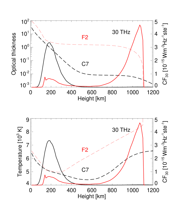
Figure 5.: Top: Opacity $\tau_{30}$ (dashed lines) and contribution function CF (solid lines) as a function of height above the photosphere. Red curves represent F2 model results, while black curves are for C7. Bottom: Atmospheric local temperature (dashed lines) and CF (solid lines) as a function of height. Fig˙c7f2

For each atmospheric model Table 3 displays h_max and $\rm{\tau_{30}}$ at the maximum of $\rm{CF_{30}}$, the altitude range $\Delta\rm{h}$ at half of the $\rm{CF_{30}}$ maximum, the expected brightness temperature $\rm{T_{b30}}$, the excess brightness temperature $\Delta\rm{T_{b30}}$ and the corresponding excess flux density $\Delta$S₃₀ (for a 10^′′ source) with respect to values obtained for C7. The dashed lines in Figure Fig_c7f2 show $\rm{\tau_{30}}$ (top) and T (bottom) as a function of h for C7 (black) and F2 (red). The corresponding height profiles of CF₃₀(h) (solid lines) are over plotted in both panels. The 30 THz emission from C7, FLA and F1 arises from an atmospheric layer LC7_l centered at h_max $\sim$ 180  km, where $\rm{\tau_{30}}\sim 1$, which extends from $\sim$ 130–140 to 270–300 km . Thus, for these models, the 30 THz radiation arises from an optically thick layer located below the temperature minimum region at temperatures around 5000 K. For the quiet Sun, this is consistent with earlier results (see e.g. Figure 2 in Deming et al., 1991). FLA and F1 cannot explain the 30 THz emission observed during SOL2012-03-13 because they lead to $\Delta$S₃₀$\sim$ 1000-1500 sfu, which is about one order of magnitude lower than the observed value $\sim$ 12,000 sfu at the maximum of the 30 THz burst. On the contrary, F2 leads to $\Delta$S₃₀ $\sim$ 12,300 sfu, which is in agreement with the observed value. In F2, the maximum of CF₃₀ occurs at h_max $\sim$ 1070 km where $\rm{\tau_{30}}$ $<$ 1 so that the 30 THz radiation arises mostly ($\sim$ 80%) from an atmospheric layer LF2, $\Delta$h_h $\sim$ 960-1100 km, located above the temperature minimum region at temperatures around 8000 K. Figure Fig_c7f2 shows that for F2, in addition to the LF2 layer, there is an optically thick 30 THz emitting layer, slightly below the temperature minimum, in the altitude range $\Delta h_{1}\sim$ 130–270 km. This latter source contributes moderately ($\sim$ 20%) to the total emission. Its temperature is a few tens of kelvin larger than that of the quiet Sun so that it represents only less than 1% of the quiet Sun emission. This is in line with earlier theoretical expectations by Ohki and Hudson (1975) which indicate that the contrast between the quiet and flare infrared emission in the 10-40 THz range is about ten times higher for an optically thin source at about 10⁴ K than for an optically thick source around 5000 K. This is also consistent with results of time-dependent numerical simulations (see Figure 3 in Kašparová et al., 2009a). The F2 flare model appears thus as a plausible atmospheric model to account for the 30 THz emission radiated during SOL2012-03-13.

7 30 THz chromospheric response to flare accelerated particles

S-Resp The 30 THz time profile (see Figure Fig_over) exhibits an impulsive emission, which encompasses the two radio and HXR peaks, superimposed on a long-lasting and slowly varying component (see Section S-Over). This suggests that the 30 THz impulsive burst results, directly or indirectly, from chromospheric heating due to energy deposition by non-thermal particles (electrons, protons and $\alpha$ particles) while the slowly varying emission is generated by some slower process like, e.g., conduction fronts. In the following we focus on the chromospheric heating by particles accelerated during SOL2012-03-13. A proper treatment of this problem, which is beyond the scope of the present study, should account for the temporal evolution of the flaring atmosphere due to time dependent heating by particles as in Kašparová et al. (2009a, b). Here, we simply consider C7 as the initial atmosphere model at t₀ $\sim$ 17:20:45 UT (beginning of the HXR and 30 THz radiation) and F2 as the atmosphere model that is reached at t₁ $\sim$ 17:24:50 UT (maximum of the observed 30 THz radiation). For a given atmosphere model we have calculated the energy deposition per centimeter by non-thermal particles $\Theta(N)$ (erg cm^-1) as a function of the hydrogen column depth $N$ (see Eq. edep3 in the Appendix). In the following we use height $h$ to parametrize altitude above the photosphere in a given atmosphere, considering $\Theta(h)$ rather than $\Theta(N)$. These computations are presented in detail in the Appendix. They extend previous works (e.g. Emslie, 1978) by considering that the degree of ionization varies with $N$ and retaining the energy-dependence of the Coulomb logarithm, which is particularly important for ions.

As a first approach, we have computed the total energy deposited by particles accelerated between t₀ and t₁ as a function of $h$ in C7. For that we have integrated the BGO count rate spectrum spectrum from t₀ to t₁ and estimated the mean flux of electrons, protons and $\alpha$ particles in the same way as in Section S-xrgr and multiplied by t${}_{1}-\rm{t}_{0}$ = 245 s . This leads to $\mathcal{F}_{0\rm{e}}(>50~{}\rm{keV})\sim 10^{37}$, $\mathcal{F}_{0\rm{p}}(>\rm{30~{}MeV})\sim 8.5\times 10^{30}$ and $\mathcal{F}_{0\rm{\alpha}}(\rm{>30~{}MeV/nucl})\sim 1.9\times 10^{30}$ for respectively the total numbers of $>$ 50 keV electrons, $>$ 30 MeV protons and $>$ 30 MeV/nucl $\alpha$ particles accelerated between t₀ and t₁. We then use these normalizations in Eq. (edep3) to calculate the energy deposited per cm due to electrons, protons and ions, and sum over these to obtain the total energy deposited by particles per cm $\rm{E^{tot}}\rm{(h)}$. Figure fig_edep shows $\rm{E}\rm^{tot}{(h)}$ as a function of h in the pre-flare atmosphere C7 for the ensemble of accelerated particles as well as the contributions from electrons, protons and $\alpha$ particles separately. As stated in Section S-30T most of the 30 THz emission arises from the LF2 layer marked by red vertical dashed lines in Figure fig_edep. The altitude range of the C7 layer LC7 (750–820 km), which covers the same range of mass column densities ($3.5\times 10^{-3}$–$6.2\times 10^{-3}$ g cm^-2) as LF2, is marked by the black dashed lines in the Figure fig_edep. Such a range of column density is consistent with that indicated by Machado, Emslie, and Avrett (1989). As a rough approximation we assume that the total energy deposited by particles between t₀ and t₁ in LC7, E${}_{\rm{par}}^{\rm{LC7}}$, may account for the 30 THz emission from LF2. By integrating $\rm{E}\rm{{}^{tot}{(h)}}$ over the LC7 altitude range we get E${}_{\rm{par}}^{\rm{LC7}}\sim 3\times 10^{29}$ erg. The total amount of energy radiated at 30 THz between t₀ and t₁ is given by:

$$\mathrm{E_{30}^{tot}=10^{-15}~{}4\pi~{}R^{2}\Delta\nu\int_{t_{0}}^{t_{1}}\Delta S_{30}(t)dt~{}\sim~{}10^{28}~{}erg},\$$ (3)

where R=1 AU=1.5 $\times$ 10¹¹ m, $\Delta\nu$ is the observed frequency bandwidth in Hz (see Section S-Inst) and $\Delta\rm{S_{30}(t)}$ the excess flux density at 30 THz in sfu. E${}_{\rm{par}}^{\rm{LC7}}$ is about thirty times larger than E${}_{\rm{30}}^{\rm{tot}}$. Thus, direct heating by non-thermal particles appears as a possible mechanism to account for the $\sim$ 80% of the impulsive 30 THz emission which arises from LF2. This latter statement remains valid even if we included a range of initial pitch angles, mirroring and pitch angle scattering in the energy deposition calculation (see Appendix). On the other hand, the energy   6$\times 10^{26}$ erg deposited by particles in LC7_l, which corresponds to about the same mass column density and altitude ranges as the equivalent layer in F2 (see Section S-30T) is too small to account for the remaining 20% of the 30 THz radiation. The heating in the LC7_l layer may thus be due to some indirect mechanism, such as radiative backwarming of the deep chromosphere from the LF2 layer (e.g., Metcalf, Canfield, and Saba, 1990; Kerr and Fletcher, 2014) or radiative coupling of the upper chromosphere and temperature minimim regions (Machado, Emslie, and Avrett, 1989). It should be noted that a harder ion distribution (e.g. $\delta=2$) would deposit a greater fraction of its total energy content in the deeper atmosphere. To this extent the calculations here, with a fixed value of $\delta=4$ should be regarded as illustrative. The statistical quality of the $\gamma$-ray spectrum for this event does not justify more detailed investigation, however.

Figure Fig_over shows that the evolution of the H$\alpha$ emission from the S₁ and S₂ kernels (see Figure Fig_images) is similar to that of the 30 THz excess flux density. Because the H$\alpha$ emission arises from a $\sim$ 10⁴ K plasma, the altitudes of S₁ and S₂ should be close to that of the 30 THz source at $\sim$ 8000 K. This suggests that direct heating by particles is also responsible for the impulsive H$\alpha$ radiation while, like for the 30 THz emission, the slowly-varying, long-lasting component is due to some other process. A detailed and quantitative analysis of the WL emission is beyond the scope of this study. Nevertheless, as remarked in Section S-Over, the WL time profile exhibits only the impulsive emission and not the slowly-varying, long-lasting component. This suggests that the mechanism responsible for the 30 THz and H$\alpha$ slowly-varying, long-lasting component is not efficient enough to produce WL emission whether it arises from direct particle heating from a LF2-like layer or from indirect heating of the deep chromosphere (LC7_l layer). The former hypothesis is consistent with the heights of WL sources, $\sim$ 800–1000 km above the photosphere estimated by e.g. Krucker et al. (2015) for some flares.

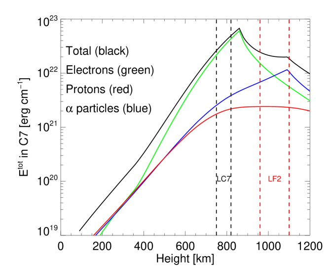
Figure 6.: Energy deposition per unit of height in C7 (E^tot) by flare accelerated particles as a function of height. The dashed vertical lines in red show the F2 atmospheric layer (LF2) from which $\sim$ 80% of the 30 THz emission arises. The black vertical lines show the C7 layer (LC7) which covers the same mass column density as the LF2 layer.fig˙edep

8 Summary

S-Sum The SOL2012-03-13 flare is the first event that have been detected in the mid-infrared domain at 30 THz (Kaufmann et al., 2013). The combined analysis of the 30 THz data with HXR/GR, WL, H$\alpha$ and 1-400 GHz radio observations has allowed us to estimate the numbers of electrons, protons and $\alpha$ particles accelerated during the flare and to discuss the origin of the 30 THz emission. The main findings can be summarized as follows:

• The HXR/GR observations of the Gamma-ray Burst Monitor on FERMI have revealed that SOL2012-03-13 is a gamma-ray line flare detected up to at least 10 MeV. The numbers and energy contents of HXR/GR emitting electrons, protons and $\alpha$ particles have been estimated. The energy content in protons and $\alpha$ particles with energies above 1 MeV/nucl. is found to be similar to the energy content in $>$ 50 keV electrons. This indicates that, in addition to electrons, protons and $\alpha$ particles may substantially contribute to the heating of the chromosphere during flares such as SOL2012-03-13.

• The observed 1–200 GHz radio spectrum is reminiscent of gyrosynchrotron radiation. The optically-thin part of the radio spectrum ($>$ 10–20 GHz) is radiated by HXR/GR emitting electrons with energies greater than $\sim$ 800 keV. The spectrum of these high energy electrons is harder than that of lower energy electrons.

• Assuming that the 30 THz emission is thermal emission from the chromosphere we have used time independent semi-empirical models of both the quiet and flaring atmospheres in order to identify from which atmospheric layers the 30 THz emission arises. In agreement with earlier works we find that the quiet Sun 30 THz radiation is emitted by an optically thick layer, at temperatures around 5000 K, below the temperature minimum region. During the flare, the measured flux density excess at 30 THz is consistent with that expected from the F2 model by Machado et al. (1980) which is representative of medium size flares. In this model, about 80% of the 30 THz emission arises from an atmospheric layer LF2 ($\sim$ 960–1100 km above the photosphere) at temperatures around 8000 K well above the temperature minimum region. At 30 THz, this layer is not optically thick ($\tau<1$). The remaining 20% of the 30 THz emission arises from an optically-thick layer, slightly below the temperature minimum region in F2, which covers similar altitude and mass column density ranges to those of the emitting layer in the quiet Sun.

• The energy deposited by electrons, protons and $\alpha$ particles in the quiet Sun layer which covers the same range of mass column density (3.5–6.2 $\times 10^{-3}$ g cm^-2) has been calculated by taking into account that the degree of ionization varies with height and by retaining the energy-dependence of the Coulomb logarithm. This energy is found to be about thirty times greater than that radiated at 30 THz. Thus energy deposition by accelerated particles is a plausible mechanism responsible for the heating of the LF2 layer which gives rise to $\sim$ 80% of the observed 30 THz emission during the impulsive phase of SOL2012-03-13. On the other hand, the energy deposited by particles in the deep chromosphere is too small to account for the remaining 20% of the 30 THz flux density radiated from below the temperature minimum region in F2. A possible, but not unique, scenario is that the impulsive WL emission and 20% of the 30 THz radiation arises from an optically-thick layer, below the temperature minimum region, heated by e.g. backwarming from the upper chromosphere where most of the energy transported by accelerated particles is deposited.

• The 30 THz and H$\alpha$ exhibit a long-lasting and slowly varying component which is not observed in the WL and HXR/GR domains. This indicates that the chromospheric heating giving rise to this component is due to a different mechanism than energy deposition by accelerated particles and that the efficiency of this mechanism is not sufficient to produce long-lasting WL emission.

In summary, using time-independent semi-empirical models of the quiet and flare atmosphere, we have shown that thermal emission from the chromosphere heated by accelerated particles provides a plausible quantitative interpretation of the 30 THz emission in gross agreement with that observed during the impulsive phase of SOL2012-03-13. Time dependent numerical models of energy deposition by accelerated particle such as developed by Kašparová et al. (2009a) are needed to confirm our conclusion. Moreover, if the 30 THz emission arises from a quasi optically-thin chromospheric layer like LF2, the emission spectrum between $\sim$ 10–100 THz is expected to be rather flat or even slightly decreasing with increasing frequencies (see Figure 2 in Ohki and Hudson, 1975). Observations at frequencies above 30 THz such as those recently obtained from the McMath-Pierce Solar Facility at Kitt Peak (Penn et al., 2015) should allow us to test the validity of such an expectation, and thus of the thermal interpretation of the infrared emission from flares proposed in this work. In the near future, the combination of McMath observations and measurements at 3 and 7 GHz by Solar-T (Kaufmann et al., 2014) should allow to complete our understanding of the chromospheric response to flare energy release.

Acknowledgements

The authors thank G. Chambe and K.-L. Klein for their suggestions and critical comments. We thank STFC for support through grant ST/L000741/1 (ALM). Some of ALM contribution was carried out while on study leave at CRAAM, Mackenzie Presbyterian University, São Paulo with FAPESP financial support. PJAS acknowledges the European Community’s Seventh Framework Programme (FP7/2007-2013) under grant agreement no. 606862 (F-CHROMA) for financial support. VDL thanks Catedras-CONACyT project 1045. This research was partially supported by Brazil agencies FAPESP (contract 2013/24155-3),CNPq (contract 312788/2013-4), Mackpesquisa and U.S. AFOSR. We are grateful to the referee, Säm Krucker, for his constructive recommendations.

app In order to compute the energy deposited by accelerated electrons, protons and $\alpha$ particles in the chromosphere as a function of depth, we inject particles with an energy spectrum $F_{0}(E)$ (MeV^-1) at the top of the atmosphere. We parametrize position in the atmosphere using the hydrogen column depth $N$. The energy deposited (erg cm^-1) at depth $N$ is (following Emslie, 1978)

$$\Theta(N)\,=\,\int_{E_{min}(N)}^{\infty}\frac{F_{0}(E_{0})}{v(E)}\left|\frac{\mathrm{d}E}{\mathrm{d}t}(E,N)\right|\mathrm{d}E_{0}.\ilabel{edep1}$$ (4)

Here $E_{min}(N)$ is the minimum energy of particle that can reach depth $N$. In Equation (edep1) $E$ should be understood as depending on $E_{0}$ and $N$: it is the energy that a particle of initial energy $E_{0}$ has when it has reached depth $N$.

An ion of energy $E$ and charge $z$ loses energy with depth at a rate given by (Gould, 1972b; Emslie, 1978; Olive and Particle Data Group, 2014)

$$\frac{\mathrm{d}E}{\mathrm{d}N}\,=\,-\frac{K}{\beta^{2}}\Lambda_{eff}(E,N)\ilabel{eloss}$$ (5)

Here $\beta$ is particle speed in units of the speed of light, $K$ is given by

$$K=\frac{4\pi e^{4}}{m_{e}c^{2}}z^{2}\,,$$

$$\Lambda_{eff}(E,N)\,=\,x\Lambda+(1-x)\Lambda^{\prime},$$ (6)

where $x$ is the degree of ionisation and $\Lambda$ and $\Lambda^{\prime}$ are the Coulomb logarithms appropriate to slowing on electrons, and on neutral atoms respectively. For ions, expressions for $\Lambda$ are given in e.g. Butler and Buckingham (1962); Gould (1972a). For $\Lambda^{\prime}$ we used the Bethe-Bloch form (Olive and Particle Data Group, 2014), neglecting the correction for the polarisation of the medium which is negligible in the low-density conditions of the solar atmosphere. We estimate the effects of the atmospheric chemical composition on energy loss by multiplying $\Lambda^{\prime}$ by

$$\sum_{n}\frac{a_{n}}{a_{H}}\frac{Z_{n}}{A_{n}}\,=\,1.16$$

where $n$ sums over atomic species and $A_{n}$, $Z_{n}$ and $a_{n}$ are the atomic number, atomic weight and abundance relative to hydrogen of species $n$. Also we generalise $x=n_{e}/n_{H}$ so that it is no longer quite the “degree of ionisation” and may take values $>1$, dependent on the local electron density.

$\Lambda$ and $\Lambda^{\prime}$ for electrons are given in Gould (1972a); Emslie (1978). In using only Equation (eloss) we neglect pitch-angle scattering. Scattering in angle is unimportant for fast ions and relativistic electrons - the only particles that can reach the LC7_l layer. For non-relativistic electrons it reduces the mean range by 2/3 (Brown, 1972), although dispersion means that electrons will stop and deposit energy over a range of depths up to their full vertical stopping depth (Bai, 1982). For the present purposes of estimation we neglect pitch-angle scattering completely.

Figure 7.: The effective Coulomb logarithm, $\Lambda_{eff}$ through the atmosphere for protons of energy 1, 10 and 100 MeV.lamplot

Figure lamplot shows the value of $\Lambda_{eff}$ throughout the chromospheric portion of the C7 atmosphere of Avrett and Loeser (2003), for protons of energies 1, 10 and 100 MeV. The importance of retaining the energy-dependence of $\Lambda$ has been emphasised elsewhere (MacKinnon and Toner, 2003). The variable degree of ionisation means that $\Lambda_{eff}$ also depends strongly on position. Thus the energy loss rate of Equation (eloss) is not separable in energy and depth, and analytical heating rates like those of Emslie (1978) may not be used (although an energy loss rate appropriate to a completely neutral atmosphere would give a good approximation below about 1000 km).

To evaluate the energy deposition $\Theta$ we need to assume a form for $F_{0}(E_{0})$, e.g. a single power law:

$$F_{0}(E_{0})\,=\,\frac{\mathcal{F}_{0}}{E_{*}}(\delta-1)\left(\frac{E_{0}}{E_{*}}\right)^{-\delta},\ilabel{eff0}$$ (7)

where $\mathcal{F}_{0}$ is the number of particles injected above energy $E_{*}$. Then applying Equation (eloss) in Equation (edep1) gives

$$\Theta(N)\,=\,8.16\times 10^{-31}z^{2}n_{H}(N)\mathcal{F}_{0}E_{*}^{\delta-1}(\delta-1)\int_{E_{min}(N)}^{\infty}E^{-\delta}\frac{\Lambda_{eff}(E,N)}{\beta^{2}(E)}\mathrm{d}E_{0}\ilabel{edep3}$$ (8)

Again, $E$ in the integrand of Equation (edep3) is understood to be a function of $E_{0}$ and $N$: the energy at depth $N$ of a particle that had energy $E_{0}$ at injection. Since we cannot obtain analytical expressions for $E(E_{0},N)$ we calculate it via numerical integration of Equation (eloss), with numerical interpolation as necessary between the tabulated points of a given atmosphere model, as needed for each of the abscissae of a numerical evaluation of the energy deposition (Equation (edep3)). More elaborate forms of $F_{0}(E_{0})$, e.g. the broken power-law deduced for electrons, are straightforwardly substituted in Equation (edep1) as necessary.

References

- Avrett and Loeser (2003) Avrett, E.H., Loeser, R.: 2003, Solar and Stellar Atmospheric Modeling Using the Pandora Computer Program. In: Piskunov, N., Weiss, W.W., Gray, D.F. (eds.) Modelling of Stellar Atmospheres, IAU Symp. 210, 21P.
- Avrett and Loeser (2008) Avrett, E.H., Loeser, R.: 2008, Models of the Solar Chromosphere and Transition Region from SUMER and HRTS Observations: Formation of the Extreme-Ultraviolet Spectrum of Hydrogen, Carbon, and Oxygen. ApJS 175, 229.
- Bagalá et al. (1999) Bagalá, L.G., Bauer, O.H., Fernández Borda, R., Francile, C., Haerendel, G., Rieger, R., Rovira, M.G.: 1999, The New H Solar Telescope at the German-Argentinian Solar Observatory. In: A. Wilson & et al. (ed.) Magnetic Fields and Solar Processes, SP-448, 469.
- Bai (1982) Bai, T.: 1982, Transport of energetic electrons in a fully ionized hydrogen plasma. ApJ 259, 341.
- Bastian, Benz, and Gary (1998) Bastian, T.S., Benz, A.O., Gary, D.E.: 1998, Radio Emission from Solar Flares. ARA&A 36, 131.
- Brown (1972) Brown, J.C.: 1972, The Directivity and Polarisation of Thick Target X-Ray Bremsstrahlung from Solar Flares. Sol. Phys. 26, 441.
- Butler and Buckingham (1962) Butler, S.T., Buckingham, M.J.: 1962, Energy loss of a fast ion in a plasma. Phys. Rev. 126, 1.
- De la Luz, Lara, and Raulin (2011) De la Luz, V., Lara, A., Raulin, J.-P.: 2011, Synthetic Spectra of Radio, Millimeter, Sub-millimeter, and Infrared Regimes with Non-local Thermodynamic Equilibrium Approximation. ApJ 737, 1.
- De la Luz et al. (2010) De la Luz, V., Lara, A., Mendoza-Torres, J.E., Selhorst, C.L.: 2010, Pakal: A Three-dimensional Model to Solve the Radiative Transfer Equation. ApJS 188, 437.
- Deming et al. (1991) Deming, D., Jennings, D.E., Jefferies, J., Lindsey, C.: 1991, In: Cox, A.N., Livingston, W.C., Matthews, M.S. (eds.) Physics of the infrared spectrum, 933.
- Emslie (1978) Emslie, A.G.: 1978, The collisional interaction of a beam of charged particles with a hydrogen target of arbitrary ionization level. Astrophys. J. 224, 241.
- Gould (1972a) Gould, R.J.: 1972a, Energy loss of a relativistic ion in a plasma. Physica 58(3), 379.
- Gould (1972b) Gould, R.J.: 1972b, Energy loss of fast electrons and positrons in a plasma. Physica 60, 145.
- Guidice (1979) Guidice, D.A.: 1979, Sagamore Hill Radio Observatory, Air Force Geophysics Laboratory, Hanscom Air Force Base, Massachusetts 01731. Report. In: Bull. Am. Astron. Soc., Bull. Am. Astron. Soc. 11, 311.
- Heinzel and Avrett (2012) Heinzel, P., Avrett, E.H.: 2012, Optical-to-Radio Continua in Solar Flares. Sol. Phys. 277, 31.
- Kaufmann et al. (2008) Kaufmann, P., Levato, H., Cassiano, M.M., Correia, E., Costa, J.E.R., Giménez de Castro, C.G., Godoy, R., Kingsley, R.K., Kingsley, J.S., Kudaka, A.S., Marcon, R., Martin, R., Marun, A., Melo, A.M., Pereyra, P., Raulin, J., Rose, T., Silva Valio, A., Walber, A., Wallace, P., Yakubovich, A., Zakia, M.B.: 2008, New telescopes for ground-based solar observations at submillimeter and mid-infrared. In: Soc. Photo-Optical Instr. Eng. (SPIE) Conf. Ser., Soc. Photo-Optical Instr. Eng. (SPIE) Conf. Ser. 7012.
- Kaufmann et al. (2013) Kaufmann, P., White, S.M., Freeland, S.L., Marcon, R., Fernandes, L.O.T., Kudaka, A.S., de Souza, R.V., Aballay, J.L., Fernandez, G., Godoy, R., Marun, A., Valio, A., Raulin, J.-P., Giménez de Castro, C.G.: 2013, A Bright Impulsive Solar Burst Detected at 30 THz. ApJ 768, 134.
- Kaufmann et al. (2014) Kaufmann, P., Marcon, R., Abrantes, A., Bortolucci, E.C., T. Fernandes, L.O., Kropotov, G.I., Kudaka, A.S., Machado, N., Marun, A., Nikolaev, V., Silva, A., da Silva, C.S., Timofeevsky, A.: 2014, THz photometers for solar flare observations from space. Exp. Astron. 37, 579.
- Kaufmann et al. (2015) Kaufmann, P., White, S.M., Marcon, R., Kudaka, A.S., Cabezas, D.P., Cassiano, M.M., Francile, C., Fernandes, L.O.T., Hidalgo Ramirez, R.F., Luoni, M., Marun, A., Pereyra, P., de Souza, R.V.: 2015, Bright 30 THz Impulsive Solar Bursts. J. Geophys. Res. 120, 4155.
- Kašparová et al. (2009a) Kašparová, J., Heinzel, P., Karlický, M., Moravec, Z., Varady, M.: 2009a, Far-IR and Radio Thermal Continua in Solar Flares. Centr. Europ. Astrophys. Bull. 33, 309.
- Kašparová et al. (2009b) Kašparová, J., Varady, M., Heinzel, P., Karlický, M., Moravec, Z.: 2009b, Response of optical hydrogen lines to beam heating. I. Electron beams. A&A 499, 923.
- Kerr and Fletcher (2014) Kerr, G.S., Fletcher, L.: 2014, Physical Properties of White-light Sources in the 2011 February 15 Solar Flare. ApJ 783, 98.
- Krucker et al. (2015) Krucker, S., Saint-Hilaire, P., Hudson, H.S., Haberreiter, M., Martinez-Oliveros, J.C., Fivian, M.D., Hurford, G., Kleint, L., Battaglia, M., Kuhar, M., Arnold, N.G.: 2015, Co-Spatial White Light and Hard X-Ray Flare Footpoints Seen Above the Solar Limb. ApJ 802, 19.
- Machado, Emslie, and Avrett (1989) Machado, M.E., Emslie, A.G., Avrett, E.H.: 1989, Radiative backwarming in white-light flares. Sol. Phys. 124, 303.
- Machado et al. (1980) Machado, M.E., Avrett, E.H., Vernazza, J.E., Noyes, R.W.: 1980, Semiempirical models of chromospheric flare regions. ApJ 242, 336.
- MacKinnon and Toner (2003) MacKinnon, A.L., Toner, M.P.: 2003, Warm thick target solar gamma -ray source revisited. A&A 409, 745.
- Marcon et al. (2008) Marcon, R., Kaufmann, P., Melo, A.M., Kudaka, A.S., Tandberg-Hanssen, E.: 2008, Association of Mid-Infrared Solar Plages with Calcium K Line Emissions and Magnetic Structures. PASP 120, 16.
- Mauas, Machado, and Avrett (1990) Mauas, P.J.D., Machado, M.E., Avrett, E.H.: 1990, The white-light flare of 1982 June 15 - Models. ApJ 360, 715.
- Meegan et al. (2009) Meegan, C., Lichti, G., Bhat, P.N., Bissaldi, E., Briggs, M.S., Connaughton, V., Diehl, R., Fishman, G., Greiner, J., Hoover, A.S., van der Horst, A.J., von Kienlin, A., Kippen, R.M., Kouveliotou, C., McBreen, S., Paciesas, W.S., Preece, R., Steinle, H., Wallace, M.S., Wilson, R.B., Wilson-Hodge, C.: 2009, The Fermi Gamma-ray Burst Monitor. ApJ 702, 791.
- Metcalf, Canfield, and Saba (1990) Metcalf, T.R., Canfield, R.C., Saba, J.L.R.: 1990, Flare heating and ionization of the low solar chromosphere. II - Observations of five solar flares. ApJ 365, 391.
- Ohki and Hudson (1975) Ohki, K., Hudson, H.S.: 1975, The solar-flare infrared continuum. Sol. Phys. 43, 405.
- Olive and Particle Data Group (2014) Olive, K.A., Particle Data Group: 2014, Review of Particle Physics. Chin. Phys. C 38(9), 090001.
- Penn et al. (2015) Penn, M., Jennings, D., Jhabvala, M., Lunsford, A.: 2015, Infrared Flare Observations at 5 and 10 Microns. In: AAS/AGU Triennial Earth-Sun Summit 1, 30704.
- Pick and Vilmer (2008) Pick, M., Vilmer, N.: 2008, Sixty-five years of solar radioastronomy: flares, coronal mass ejections and Sun Earth connection. A&A Rev. 16, 1.
- Pick, Klein, and Trottet (1990) Pick, M., Klein, K.-L., Trottet, G.: 1990, Meter-decimeter and microwave radio observations of solar flares. ApJS 73, 165.
- Ramaty (1969) Ramaty, R.: 1969, Gyrosynchrotron Emission and Absorption in a Magnetoactive Plasma. ApJ 158, 753.
- Ramaty et al. (1994) Ramaty, R., Schwartz, R.A., Enome, S., Nakajima, H.: 1994, Gamma-ray and millimeter-wave emissions from the 1991 June X-class solar flares. ApJ 436, 941.
- Scherrer et al. (2012) Scherrer, P.H., Schou, J., Bush, R.I., Kosovichev, A.G., Bogart, R.S., Hoeksema, J.T., Liu, Y., Duvall, T.L., Zhao, J., Title, A.M., Schrijver, C.J., Tarbell, T.D., Tomczyk, S.: 2012, The Helioseismic and Magnetic Imager (HMI) Investigation for the Solar Dynamics Observatory (SDO). Sol. Phys. 275, 207.
- Schwartz et al. (2002) Schwartz, R.A., Csillaghy, A., Tolbert, A.K., Hurford, G.J., McTiernan, J., Zarro, D.: 2002, RHESSI Data Analysis Software: Rationale and Methods. Sol. Phys. 210, 165.
- Trottet and Klein (2013) Trottet, G., Klein, K.-L.: 2013, Far infrared solar physics . Mem. Soc. Astron. It. 84, 405.
- Trottet et al. (1998) Trottet, G., Vilmer, N., Barat, C., Benz, A., Magun, A., Kuznetsov, A., Sunyaev, R., Terekhov, O.: 1998, A multiwavelength analysis of an electron-dominated gamma-ray event associated with a disk solar flare. A&A 334, 1099.
- Trottet et al. (2000) Trottet, G., Rolli, E., Magun, A., Barat, C., Kuznetsov, A., Sunyaev, R., Terekhov, O.: 2000, The fast and slow H chromospheric responses to non-thermal particles produced during the 1991 March 13 hard X-ray/gamma-ray flare at ~ 08 UTC. A&A 356, 1067.
- Trottet et al. (2008) Trottet, G., Krucker, S., Lüthi, T., Magun, A.: 2008, Radio Submillimeter and -Ray Observations of the 2003 October 28 Solar Flare. ApJ 678, 509.
- Valio et al. (2013) Valio, A., Kaufmann, P., Giménez de Castro, C.G., Raulin, J.-P., Fernandes, L.O.T., Marun, A.: 2013, POlarization Emission of Millimeter Activity at the Sun (POEMAS): New Circular Polarization Solar Telescopes at Two Millimeter Wavelength Ranges. Sol. Phys. 283, 651.