Universality of market superstatistics

We use a continuous-time random walk (CTRW) to model market fluctuation data from times when traders experience excessive losses or excessive profits. We analytically derive “superstatistics” that accurately model empirical market activity data (supplied by Bogachev, Ludescher, Tsallis, and Bunde) that exhibit transition thresholds. We measure the interevent times between excessive losses and excessive profits, and use the mean interevent time as a control variable to derive a universal description of empirical data collapse. Our superstatistic value is a weighted sum of two components, (i) a power-law corrected by the lower incomplete gamma function, which asymptotically tends toward robustness but initially gives an exponential, and (ii) a power-law damped by the upper incomplete gamma function, which tends toward the power-law only during short interevent times. We find that the scaling shape exponents that drive both components subordinate themselves and a “superscaling” configuration emerges. We use superstatistics to describe the hierarchical activity when component (i) reproduces the negative feedback and component (ii) reproduces the stylized fact of volatility clustering. Our results indicate that there is a functional (but not literal) balance between excessive profits and excessive losses that can be described using the same body of superstatistics, but different calibration values and driving parameters.

1 Introduction

Financial markets fluctuate as traders estimate risk levels and strive to make a profit. The interevent interval between times when market returns are producing excessive profits and times when they are producing excessive losses can be described using a continuous-time random walk (CTRW) formalism (see Refs.  (?, ?, ?, ?) and references therein).

Empirical market data on excessive profits and losses  (?, ?, ?, ?) define excessive profits as those greater than some positive fixed threshold $Q$ and excessive losses as those below some negative threshold $-Q$. The mean interevent time between losses versus $Q$ has been used as an aggregated basic variable.

Interevent times constitute a universal stochastic measurement of market activity on timescales that range from one minute to one month  (?, ?). The mean interevent time can be used as a control variable that produces a universal description of empirical data collapse  (?), i.e., the distribution of interevent times for a fixed mean interevent time is a universal statistical quantity unaffected by time scale, type of market, asset, or index.

This distribution can be described using (i) the CTRW valley model (see Refs.  (?, ?) and references therein), which treats time intervals as random variables, and (ii) generalized extreme value statistics for stochastic dependent basic processes  (?), which are $q$-exponentials not ad hoc statistics  (?, ?). Inter-event times in a multifractal structure of financial markets  (?, ?) and in the single-step memory in order-book transaction dynamics  (?) are foundational in the analysis of double-action market activity.

2 Principal goal

Our principal goal is to model the empirical data associated with single-variable statistics, i.e., (i) the mean inter-event time period $R_{Q}$ between extreme (excessive) losses, defined as those below a negative threshold $-Q$, as a function of the $Q(>0)$ value and (ii) the distribution $\psi_{Q}(\Delta_{Q}t)$ of inter-event times between losses $\Delta_{Q}t$, previously described using ad hoc $q$-exponentials.

Because no empirical data associated with item (i) are available, in our study of excessive profits we will focus on item (ii) and use the empirical data provided in Refs.  (?, ?, ?, ?). Note that the $q$-exponentials used in Refs.  (?, ?, ?, ?) cannot produce the key empirical data in item (i), and thus in our approach we use superstatistics. Because small losses and profits are of little concerm to traders, we focus on medium to high $Q$-values. Our goal is to provide market superstatistics that have universality.

3 Basic achievement

We here find an analytical closed form of the mean interevent time period $R_{Q}$ between excessive (extreme) losses that is greater than some threshold $Q$, i.e.,

$$\tau R_{Q}^{-1}=P(-\varepsilon\leq-Q)=P(\varepsilon\geq Q)=\int_{Q}^{\infty}D(\varepsilon)d\varepsilon,$$ (1)

where $\tau$ is a time unit and $D(\varepsilon)$ the density of returns given by the Weibull distribution of extreme (or excessive) losses  (?, ?, ?),

$$D(\varepsilon)=\frac{\eta}{\bar{\varepsilon}}\left(\frac{\varepsilon}{\bar{\varepsilon}}\right)^{\eta-1}\exp\left(-\left(\frac{\varepsilon}{\bar{\varepsilon}}\right)^{\eta}\right),\;\bar{\varepsilon},\;\eta>0.$$ (2)

Note that we consider random variable $\varepsilon$ to be an increment of some underlying stochastic process. Values of this random variable can, in general, be dependent  (?). Here we consider case $\eta<1$ (see Table 1) which means that distribution $D(\varepsilon)$ is, for $\varepsilon/\bar{\varepsilon}\gg 1$, a decreasing truncated power-law  (?).

Reference  (?) uses the Weibull distribution to describe the statistics of interevent times between subsequent transactions for a given asset. We use the Weibull distribution and the conditional exponential distribution of the CTRW valley model to derive superstatistics or complex statistics associated with the threshold of excessive losses or profits.

Substituting (2) into (1), we obtain

$$R_{Q}=\exp\left(\left(\frac{Q}{\bar{\varepsilon}}\right)^{\eta}\right),$$ (3)

i.e., $\ln R_{Q}$ increases vs. the relative variable $Q/\bar{\varepsilon}$ according to a power-law.

The solid curves in Fig. 1 indicate the predictions generated by (3) and fit the empirical data (the points are represented by different marks). This basic agreement enables us to construct the corresponding superstatistics and allows us to study the successive empirical data (given in Secs. 4 and 5). Because the statistical error is low we are able to determine $\eta$ and $\bar{\varepsilon}$ and derive the subsequent parameters that define the shape of the superstatistics. For example, the empirical data in Fig. 1 indicates that the value of the shape parameter exponent is $\eta<1$ (cf. Table 1), which for large losses or profits (i.e., $\varepsilon\gg\bar{\varepsilon}$) makes the Weibull distribution (2) a stretched exponentially truncated power-law. In contrast, the results presented in Ref.  (?) are incomplete because they allow no analogous comparison with theoretical predictions based on the $q$-exponential.

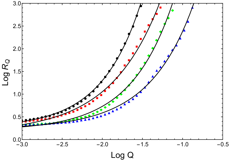
Figure 1: Mean interevent time period $R_{Q}$ vs. threshold $Q$ for four typical classes of quotations. Black circles, red squares, green rhomboids, and blue triangles concern US/GBP exchange rate, S&P 500 index, IBM stock, and WTI (the crude oil) empirical data (from January 2000 to June 2010), respectively, taken from Fig. 2 in ref.  (?) (plotted from the top curve down to the bottom one.) The solid, well fitted curves present predictions of our formula (3) - values of their fitted parameters $\bar{\varepsilon}$ and $\eta$ are shown in tab. 1 (the unimportant multiplicative calibration parameter is not presented there). Subtle wavy deviations from these predictions are not considered in this work. (Empirical data were used by permission of the EPL.)

Table 1: Values of exponent $\eta$ and quantity $\bar{\varepsilon}$ obtained from the fit of predictions of formula (3) to the empirical data (all of them plotted in Fig. 1) representing the exchange rate US Dollar against Great British Pound, the index S&P 500, the IBM stock, and crude oil (WTI).

Index/Par.	$\eta$	$\bar{\varepsilon}$
US/GBP	0.8756$\pm$0.0156	0.0037$\pm$0.0003
S&P500	0.6981$\pm$0.0292	0.0035$\pm$0.0005
IBM	0.8246$\pm$0.0236	0.0078$\pm$0.0007
WTI	0.7855$\pm$0.0182	0.0131$\pm$0.0008

4 Superstatistics

We next construct an unnormalized, unconditional distribution $\psi_{Q}(\Delta_{Q}t)$ of the interevent time stochastic variable, $\Delta_{Q}t$, in the form of superstatistics based on the Weibull distribution used in Sec. 3,

$$\psi_{Q}(\Delta_{Q}t)=\int_{Q}^{\infty}\psi_{Q}(\Delta_{Q}t|\varepsilon)D(\varepsilon)d\varepsilon.$$ (4)

Here we assume the conditional distribution $\psi_{Q}(\Delta_{Q}t|\varepsilon)$ is in the exponential form

$$\psi_{Q}(\Delta_{Q}t|\varepsilon)=\frac{1}{\tau_{Q}(\varepsilon)}\exp\left(-\frac{\Delta_{Q}t}{\tau_{Q}(\varepsilon)}\right).$$ (5)

Because it is conditional, the next (subsequent) loss is exactly $\varepsilon$, and the relaxation time is given by the stretched exponential

$$\tau_{Q}(\varepsilon)=\tau_{Q}(0)\exp\left((B_{Q}\varepsilon)^{\eta}\right)$$ (6)

as a straightforward extension of the exponential relaxation time used in the canonical version of the CTRW introduced by  (?, ?, ?, ?) in the context of photocurrent relaxation in amorphous films. Here $\tau_{Q}(0)$ is a free ($\varepsilon$-independent) relaxation time, and quantity $B_{Q}(>0)$ is independent of variable $\varepsilon$. Quantity $B_{Q}$ is a formal analog of an inverse temperature and we will later derive its scaling with the control threshold $Q$ value. We use the $\eta$ exponent in (2) to reduce the number of free exponents in (6) (Ockham’s razor principle) and to derive superstatistics $\psi_{Q}(\Delta_{Q}t)$ in an exact closed analytical form. Note that the stochastic dependence of interevent time $\Delta_{Q}t$ on loss $\varepsilon$ assumed in (5) is confirmed when smaller losses appear more frequently than larger ones. This is described by definition (6) in which mean time $\langle\Delta_{Q}t\rangle_{\varepsilon}=\tau_{Q}(\varepsilon)$ is a monotonically increasing function of $\varepsilon$. This creates an expanding hierarchy of interevent times where larger losses and profits appear less frequently than smaller ones. To make larger losses or profits appear more frequently than smaller ones, we create the opposite hierarchy of losses and profits using

$$\tau_{Q}^{\prime}(\varepsilon)=\tau_{Q}(0)\exp\left(-(B_{Q}\varepsilon)^{\eta}\right).$$ (7)

In this opposite case (which is also analytically solvable) we encounter a clustering phenomenon in which shorter time intervals separate the larger values of losses/profits rather than the smaller ones. This complementary case is briefly discussed in Sec. 5.

Substituting (6) and (5) into (4) we finally derive a superstatistics in the searched form

$$\psi_{Q}(\Delta_{Q}t) = \frac{1}{\tau_{Q}(Q)}\frac{\alpha_{Q}}{(\Delta_{Q}t/\tau_{Q}(Q))^{1+\alpha_{Q}}}$$ (8)

$$\times {\bf\gamma}_{Euler}(1+\alpha_{Q},\Delta_{Q}t/\tau_{Q}(Q)),$$

where the scaling shape exponent

$$\alpha_{Q}=\frac{1}{(B_{Q}\bar{\varepsilon})^{\eta}}=\frac{1}{\ln\left(\tau_{Q}(\bar{\varepsilon})/\tau_{Q}(0)\right)},$$ (9)

and the lower incomplete gamma function

$${\bf\gamma}_{Euler}(1+\alpha_{Q},\Delta_{Q}t/\tau_{Q}(Q))=\int_{0}^{\Delta_{Q}t/\tau_{Q}(Q)}y^{\alpha_{Q}}\exp(-y)dy.$$ (10)

The significant step in the derivation of formula (8) is the replacement of the running variable $\varepsilon$, present in the integration (4), with a new running variable $y=\Delta_{Q}t/\tau_{Q}(\varepsilon)$. This changes the stretched exponential to exponential in the overall function under the integral in (4) making the integration a straightforward (exact and closed) operation. Note that the first equality in (9) gives a straightforward, formal generalization of the corresponding exponent obtained within the canonical CTRW valley model  (?, ?, ?, ?), where $B_{Q}$ is the thermodynamic $\beta$, $\bar{\varepsilon}$ is the mean valley depth, and the exponent value is $\eta=1$.

Equation (8) asymptotically (for $\Delta_{Q}t/\tau_{Q}(Q)\gg 1$) takes a power-law form

$$\psi_{Q}(\Delta_{Q}t)\approx\frac{1}{\tau_{Q}(Q)}\frac{\alpha_{Q}}{(\Delta_{Q}t/\tau_{Q}(Q))^{1+\alpha_{Q}}}{\bf\Gamma}_{Euler}(1+\alpha_{Q})$$ (11)

of the relative interevent time $\Delta_{Q}t/\tau_{Q}(Q)$ while initially (for $\Delta_{Q}t/\tau_{Q}(Q)\ll 1$) it takes an exponential form

$$\psi_{Q}(\Delta_{Q}t)\approx\frac{1}{\tau_{Q}(Q)}\frac{\alpha_{Q}}{1+\alpha_{Q}}\exp\left(-\frac{1+\alpha_{Q}}{2+\alpha_{Q}}\Delta_{Q}t/\tau_{Q}(Q)\right).$$ (12)

For $\alpha_{Q}\gg 1$, Eq. (8) reduces to the $\alpha_{Q}$-independent exponential

$$\psi_{Q}(\Delta_{Q}t)\approx\frac{1}{\tau_{Q}(Q)}\exp\left(-\Delta_{Q}t/\tau_{Q}(Q)\right),$$ (13)

which is consistent with Eq. (12).

Note that our approach is based solely on the relaxation time (6) as a function of a single variable $\varepsilon$. Only $\varepsilon=0,\bar{\varepsilon},Q$, is used, and parameter $Q$ is the external control threshold, i.e., by using (6) and (3), we obtain

$$\ln R_{Q}=\frac{\ln\left(\tau_{Q}(Q)/\tau_{Q}(0)\right)}{\ln\left(\tau_{Q}(\bar{\varepsilon})/\tau_{Q}(0)\right)}.$$ (14)

Thus using (9) and (3) we find

$$\frac{\tau_{Q}(Q)}{\tau_{Q}(0)}=R_{Q}^{1/\alpha_{Q}}.$$ (15)

Equations (9) and (14) show the decisive role of the relaxation time $\tau_{Q}(\varepsilon)$, but its ab initio derivation is difficult. Note that Fig. 2 and Table 2 show a data collapse for a given (fixed) value of a single control (aggregated) variable $R_{Q}$.

Figure 2: Collected plots of empirical distributions (colored marks) and theoretical superstatistics, $\psi_{Q}(\Delta_{Q}t)$, (black solid curves), which are predictions of our formula (8) (while the dashed curves were given by q-exponential shown by eq. (3) in  (?)) vs. interevent time, $\Delta_{Q}t$, for the monthly returns (a), for the relative daily price returns for sixteen typical examples of financial data in the period 1962-2010 (b), from minutes over the hours to daily returns for NASDAQ between March 16, 2004 and June, 2006 (c), and for the detrended minute-by-minute eight most typical examples of financial data (d). (All empirical data were drawn from  (?, ?) for permission of EPL and PRE.)

Table 2: Values of exponent $\alpha_{Q}$ and quantity $\tau_{Q}(Q)$ obtained from the fit of formula (8) to the empirical data representing companies shown in Fig. 2 in plots (a), (b), (c) and (d) for $R_{Q}=$2, 5, 10, 30, 70.

	Fig. 2(a)		Fig. 2(b)		Fig. 2(c)		Fig. 2(d)
$R_{Q}$	$\alpha_{Q}$	$\tau_{Q}(Q)$	$\alpha_{Q}$	$\tau_{Q}(Q)$	$\alpha_{Q}$	$\tau_{Q}(Q)$	$\alpha_{Q}$	$\tau_{Q}(Q)$
2	1000	1.7699	1000	1.5436	1000	1.6129	1000	1.6129
5	3.50	3.125	2.30	2.70	3.30	3.330	3.60	3.70
10	2.10	5.0	2.0	5.0	2.0	4.550	2.10	5.0
30	-	-	1.050	5.560	1.0	5.0	1.10	5.260
70	-	-	0.550	4.760	0.550	6.670	0.50	5.260

We analytically prove that $R_{Q}$ is the control variable that allows a universal form of (8) that depends solely on $R_{Q}$. This variable was similarly used previously in connection with the $q$-exponential  (?). Using this universal form requires that we assume that the $B_{Q}$ in (6) and (9)) depends on $Q$ in a power-law form, or the relevant scaling relation of scaling variable $Q$,

$$B_{Q}=B^{1/\eta}\frac{Q^{\zeta}}{\bar{\varepsilon}^{1+\zeta}}=\frac{B^{1/\eta}}{\bar{\varepsilon}}\ln^{\zeta/\eta}R_{Q},$$ (16)

where prefactor $B$ and exponent $\zeta$ are $Q$-independent positive control parameters. Note that the second equality is a scaling relation having $\ln R_{Q}$ as a scaling variable. Thus from (9), (3), and (16) we obtain the superscaling of the scaling variable $\ln R_{Q}$ (or the scaling of scaling, i.e., the scaling of the scaling exponent),

$$\frac{1}{\alpha_{Q}}=B\ln^{\zeta}R_{Q},$$ (17)

which we further verify by examining data, e.g., for the IBM company, which are typical of the empirical data used.

From (6), (3), and (15) we next obtain the scaling relation of the scaling variable $\ln R_{Q}$,

$$\frac{\tau_{Q}(Q)}{\tau_{Q}(0)}=\exp\left(\ln^{1+\zeta}R_{Q}^{B^{1/(1+\zeta)}}\right)\Leftrightarrow\ln\left(\tau_{Q}(Q)/\tau_{Q}(0)\right)=B\ln^{1+\zeta}R_{Q}.$$ (18)

Note that quantities $B_{Q}$, $\frac{1}{\alpha_{Q}}$, and $\frac{\tau_{Q}(Q)}{\tau_{Q}(0)}$ all depend on the single control variable $\ln R_{Q}$. We will describe and discuss the $R_{Q}$-dependence of $\tau_{Q}(0)$ below, and will use the corresponding empirical data to confirm all the $R_{Q}$-dependencies.

4.1 Empirical verification of our formulas

Figure 3 shows the agreement between the predictions of (8) and the empirical data for IBM for $R_{Q}=2$, 5, 10, 30, and 70.

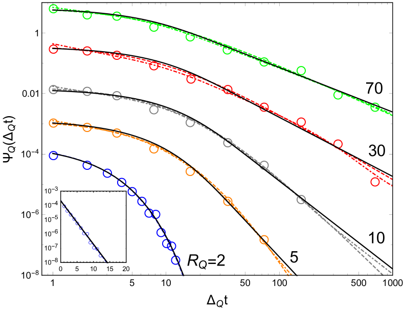
Figure 3: The superstatistics, $\psi_{Q}(\Delta_{Q}t)$, vs. interevent time, $\Delta_{Q}t$, in log-log scale for the daily price returns of IBM (empty colored circles) in the period 1962-2010 for $R_{Q}$=2, 5, 10, 30 and 70 (in units of days). Black solid curves are predictions of our formula (8) while the dashed curves were given by q-exponential shown by eq. (3) in  (?). The dashed-dotted curves are considered in Sec. 5. For $R_{Q}\geq 5$ the power-law relaxation of $\psi_{Q}(\Delta_{Q}t)$ is well seen for $\Delta_{Q}t>30$. The inset is the plot of $\psi_{Q}(\Delta_{Q}t)$ vs. $\Delta_{Q}t$ in the semi-logarithmic scale for $R_{Q}$=2 to clearly present the exponential form of the superstatistics. This exponential form was expected due to eq. (13) as $\alpha_{Q}$ is very large in this case (see tab. 3). (Empirical data were drawn from  (?) for permission of EPL.)

Table 3 shows the fit of quantities $\alpha_{Q}$ and $\tau_{Q}(Q)$.

Table 3: Values of exponent $\alpha_{Q}$ and quantity $\tau_{Q}(Q)$ obtained directly from the fit of formula (8) to the empirical data representing IBM company shown in Fig. 3 for $R_{Q}$=2, 5, 10, 30, and 70.

$R_{Q}$	$Q$	$\alpha_{Q}$	$\tau_{Q}(Q)$
2	0.0050	1000	1.4286
5	0.01389	3.0	3.330
10	0.02145	1.90	5.0
30	0.03442	0.950	4.550
70	0.04508	0.470	3.850

Figure 4(a) shows the good fit of (17) (solid curve) to the data (black circles) also found in the third column in Table 3.

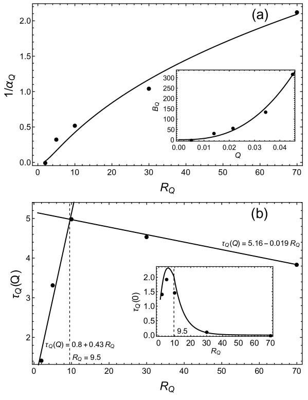
Figure 4: Key dependence of quantities: (a) $1/\alpha_{Q}$ and (b) $\tau_{Q}(Q)$ vs. $R_{Q}$ obtained, for instance, for the IBM company. Black circles in main plots represent empirical data (shown in tab. 3), while solid curves are theoretical predictions. For (a) the solid curve was obtained by the fit of formula (17) to empirical data, where the fit parameters $B$ and $\zeta$ were shown in tab. 4. The indirect empirical data for the inset plot were found from eq. (9), where $\alpha_{Q}$ was taken from tab. 3, while $\eta$ and $\bar{\varepsilon}$ from tab. 1 for the IBM company. The solid curve in this inset plot is the prediction of eq. (16) for mentioned above parameters $B$ and $\zeta$. For (b) the broken line or both solid straight lines are linear regressions (i.e. given by $\tau_{Q}(Q)=a_{s}\,R_{Q}+b_{s},\;\mbox{where}\;s=L\;\mbox{for the lhs straight line}$ and $s=R\;\mbox{for the rhs straight line}$; here $\tau_{0}(0)=a_{L}+b_{L}=1.24$ as $R_{Q=0}=1$). Multiplicative and additive calibration parameters $a_{s}$ and $b_{s}$ defining both straight lines are shown in tab. 6. Hence, we have an additional interpretation of $\tau_{Q}(Q)$ as equal $R_{Q}$ up to some multiplicative and additive calibration parameters. The solid curve in the inset plot (i.e. $\tau_{Q}(0)$ vs. $R_{Q}$) was obtained from formula (18), where $B$ and $\zeta$ comes from tab. 4, while $\tau_{Q}(Q)$ was defined by above given straight lines.

This fit allows us to determine the parameter $B$ and exponent $\zeta$ (see Table 4).

Table 4: Universal parameter $B$ and universal exponent $\zeta$, defining dependence of $B_{Q}$ vs. $Q$, obtained from the good fit of formula (17) (solid curve) to the empirical data (black circles) shown in Fig. 4a, for instance, for very representative IBM company.

$B$	$\zeta$
0.04798$\pm 0.0249$	2.6096$\pm 0.3478$

The inset plot shows the good agreement between the (16) prediction (solid curve) and the data (black circles). We prepared the data by putting the first equality in (9) into the third column of Table 5, where the $\bar{\varepsilon}$ and $\eta$ of IBM is supplied in Table 1.

Table 5: Values of elementary quantities $B_{Q}$ and $\tau_{Q}(0)$ derived from key quantities $\alpha_{Q}$ and $\tau_{Q}(Q)$ found from the fit of formula (8) to the empirical data representing IBM company shown in Fig. 3 for $R_{Q}$=2, 5, 10, 30, and 70 for $\eta$=0.8246 and $\bar{\varepsilon}$=0.0078 given in tab. 1.

$R_{Q}$	$Q$	$B_{Q}$	$\tau_{Q}(0)$
$2$	$0.0050$	$0.0295$	$1.4286$
$5$	$0.01389$	$33.82951$	$1.94745$
$10$	$0.02145$	$58.86516$	$1.48793$
$30$	$0.03442$	$136.43324$	$1.26807\times 10^{-1}$
$70$	$0.04508$	$320.29882$	$4.56615\times 10^{-4}\approx 0$

Figure 4(b) shows a plot of $\tau_{Q}(Q)$ vs. $Q$, where $\tau_{Q}(Q)$ comes from the fourth column of Table 3. The plot consists of a broken straight line or two crossing straight lines. Table 6 shows the parameters of linear regressions $a_{s}$ and $b_{s}$, with $s=L,R$, that define the dependence of both straight lines on $R_{Q}$. The inset plot uses (15) and (17) to calculate (i) the data points (black circles) with $\tau_{Q}(Q)$ supplied by Table 3, and (ii) the solid curve, using the analytical form of $\tau_{Q}(Q)$.

Table 6: Parameters of linear regressions $a_{s}$ and $b_{s}$, $s=L,R$, defining dependence of both straight lines on $R_{Q}$, presented in Fig. 4b for the IBM company.

Parameters	$L$	$R$
$a_{s}$	0.430	-0.019
$b_{s}$	0.80	5.160

Thus by analytically and empirically proving the $R_{Q}$-dependence of the superstatistics $\psi_{Q}(\Delta_{Q}t)$ we explain the empirical data collapse shown in Fig. 2.

5 Discussion and concluding remarks

We find an explicit closed form of the threshold interevent time superstatistics (8) that is valid for excessive losses, is the foundation of the continuous time random walk (CTRW) formalism, and that is useful in the study of a double action market (see  (?) and refs. therein). These superstatistics are more credible than the $q$-exponential distribution that is applied ad hoc in this context in Ref.  (?, ?), and they agree with the key empirical relation between the mean interevent time $R_{Q}$ and the threshold $Q$ (see Fig. 1).

We model the empirical data collapse (cf. Fig. 2) using superstatistics as a function of a single aggregated variable $R_{Q}$ and obtain, for example, the scaling shape exponent $1/\alpha_{Q}$ as a power-law function of $\ln R_{Q}$ and the superscaling form of (17) that is dependent upon universal exponent $\zeta$ and prefactor $B$.

Note that (8) accurately describes the empirical statistics of excessive profits. Here $Q$ defines the threshold for excessive profits instead of excessive losses (see the plots in Fig. 5). We thus can use the same superstatistics to demonstrate the functional but not literal symmetry between excessive losses and profits. The symmetry is not literal because different control parameters $B$ and $\zeta$ and driving parameters $a_{s}$ and $b_{s}$ ($s=L,R$) are used. Because of large statistical errors in the empirical data, we cannot empirically verify the universality of excessive profit behavior. For example, for $R_{Q}=10$ exponent $1.70\leq\alpha_{Q}\leq 3.10$ and $0.10\leq\tau_{Q}(Q)\leq 0.25$, for $R_{Q}=30$ we have $0.90\leq\alpha_{Q}\leq 1.50$ and $0.12\leq\tau_{Q}(Q)\leq 0.35$, and finally for $R_{Q}=70$ we have $0.60\leq\alpha_{Q}\leq 1.10$ and $0.08\leq\tau_{Q}(Q)\leq 0.36$, which exhibit ranges that are too extended.

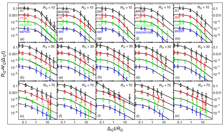
Figure 5: Statistics of interevent times between arithmetic profit returns of daily closing for various markets (from stock exchange and forex to resource market) and time periods. All empirical data (discrete marks with bars) were taken from ref.  (?). Solid curves are predictions of our formula (8) as it can be applied both for losses and profits. Dashed curves shown, for instance, in plots (a), (b), and (c) are fitted by q-exponential (remaining twelve plots are very similarly fitted therefore, the fits are not visualized herein). However, the possible empirical data collapse would be incredible in this case because errors of empirical data points are too large. (Empirical data were drawn from  (?) for permission of PRE.)

Note that if we substitute $\tau_{Q}^{\prime}(\varepsilon)$ given by (7)—the case opposite to that defined by (6)—into (5), and use a derivation analogous to the one that produced (8), we obtain a result complementary to (8), i.e.,

$$\psi_{Q}^{\prime}(\Delta_{Q}t) = \frac{1}{\tau_{Q}^{\prime}(Q)}\frac{\alpha_{Q}}{(\Delta_{Q}t/\tau_{Q}^{\prime}(Q))^{1+\alpha_{Q}}}$$ (19)

$$\times {\bf\gamma}_{Euler}^{\prime}(1+\alpha_{Q},\Delta_{Q}t/\tau_{Q}^{\prime}(Q)),$$

where

$${\bf\gamma}_{Euler}^{\prime}(1+\alpha_{Q},\Delta_{Q}t/\tau_{Q}^{\prime}(Q))=\int_{\Delta_{Q}t/\tau_{Q}^{\prime}(Q)}^{\infty}y^{\alpha_{Q}}\exp(-y)dy$$ (20)

$$= {\bf\Gamma}_{Euler}(1+\alpha_{Q})-{\bf\gamma}_{Euler}(1+\alpha_{Q},\Delta_{Q}t/\tau_{Q}^{\prime}(Q)),$$

is the upper gamma function, which for $\Delta_{Q}t/\tau_{Q}^{\prime}(Q)\gg 1$ truncates the power-law in (19). In the opposite case of $\Delta_{Q}t/\tau_{Q}^{\prime}(Q)\ll 1$ we obtain

$$\psi_{Q}^{\prime}(\Delta_{Q}t)\approx\frac{1}{\tau_{Q}^{\prime}(Q)}\frac{\alpha_{Q}}{(\Delta_{Q}t/\tau_{Q}^{\prime}(Q))^{1+\alpha_{Q}}}{\bf\Gamma}_{Euler}(1+\alpha_{Q}),$$ (21)

which is only formally identical to (11). Figure 3 shows the best predictions of the weighted sum of superstatistics (dashed dotted curves) given by (8) and (19). Note that this continues to agree with the corresponding empirical data for IBM.

We use (2), (6), and (9) to obtain the moment $\langle(\Delta_{Q}t)^{m}\rangle,\,m=0,1,2,\ldots$ in an explicit closed form,

$$\langle(\Delta_{Q}t)^{m}\rangle = \frac{\int_{0}^{\infty}(\Delta_{Q}t)^{m}\,\psi_{Q}(\Delta_{Q}t)d(\Delta_{Q}t)}{\int_{Q}^{\infty}D(\varepsilon)d\varepsilon}$$ (22)

$$= \frac{m!\int_{Q}^{\infty}[\tau_{Q}(\varepsilon)]^{m}D(\varepsilon)d\varepsilon}{\int_{Q}^{\infty}D(\varepsilon)d\varepsilon}$$

$$= R_{Q}(\tau_{Q}(Q))^{m}\frac{m!}{1-m/\alpha_{Q}},\;\;m=0,1,2,\ldots,$$

where the first equality gives the definition. Note that the moments of arbitrary order, as well as $\alpha_{Q}$ and $\tau_{Q}(Q)$, depend solely on $R_{Q}$. Note also that $\langle(\Delta_{Q}t)^{m}\rangle$ is finite only for $\alpha_{Q}>m$, and that otherwise it diverges. This is in contrast to the behavior of $R_{Q}$, which, because of its quantile (not momentum) origin, is always finite, e.g., for IBM $\langle\Delta_{Q}t\rangle$ is finite only for $R_{Q}\leq 10$ (see Table 3). We thus have two radically different cases, finite interevent time and infinite interevent time $\langle\Delta_{Q}t\rangle$, about which there is much in the literature (see, e.g.,  (?, ?, ?, ?) and refs. therein). Infinite interevent time is particularly interesting when it takes into consideration ergodicity breaking  (?, ?).

Note that using our microscopic model to simulate agent behavior  (?, ?) gives results very close to those predicted by (8). An approach using agent-based modeling in this context was recently explored by other authors  (?).

It is our hope that this work will constitute a strong contribution to the research effort searching for universal properties in market behavior.

• Acknowledgments Two of us (M.J. and T.G.) are grateful to the Foundation for Polish Science for financial support. The work of H.E.S. was supported by NSF Grant CMMI 1125290, DTRA Grant HDTRA1-14-1-0017 and ONR Grant N00014-14-1-0738. One of us (R.K.) is grateful for inspiring discussions with Shlomo Havlin (during The Third Nikkei Econophysics Symposium, Tokyo 2004), Armin Bunde (during his visit at Faculty of Physics University of Warsaw in 2011), and Constantino Tsallis (during the SMSEC2014 in Kobe).

References and Notes

- 1. G. Pfister and H. Scher, Adv. Phys. 27, 747 (1978).
- 2. J. W. Haus and K. W. Kehr, Phys. Rep. 150, 263 (1987).
- 3. R. Kutner and F. Świtała, Quant. Finance 3, 201 (2003).
- 4. T. Sandev, A. Chechkin. H. Kantz. R. Mentzler, An Int. J. Theory and Applications 18, 1006 (2015).
- 5. J. Ludescher, C. Tsallis, A. Bunde, Eur. Phys. Let. 95, 68002 (2011).
- 6. J. Ludescher and A. Bunde, Phys. Rev. E 90, 062809 (2014).
- 7. M. I. Bogachev and A. Bunde, Phys. Rev. E 78, 036114 (2008).
- 8. M. I. Bogachev and Bunde, Phys. Rev. E 80, 026131 (2009).
- 9. K. W. Kehr, R. Kutner, K. Binder, Phys. Rev. B 23, 4931 (1981).
- 10. E. Bertin and M. Clusel, J. Phys. A: Math. Gen. 39, 7607 (2006).
- 11. J. Perelló, J. Masoliver, A. Kasprzak, and R. Kutner, Phys. Rev. E 78, 036108 (2008).
- 12. A. Kasprzak, R. Kutner, J. Perelló, J. Masoliver, Eur. Phys. J. B 76, 513 (2010).
- 13. T. Gubiec and R. Kutner, Phys. Rev. E 82, 046119 (2010).
- 14. Y. Malevergne and D. Sornette, Extreme Financial Risks. From Dependence to Risk Management (Springer-Verlag, Berlin, 2006).
- 15. P. Embrechts, C. Klüppelberg C., Th, Mikosch, Modelling Extremal Events for Insurance and Finance (Springer-Verlag, Berlin, 1997).
- 16. J. Franke, W. Härdle, Ch. Hafner, Statistics of Financial Markets, (Springer-Verlag, Berlin, 2004).
- 17. B. B. Mandelbrot, Fractals and Scaling in Finance (Springer-Verlag, New York, 1997).
- 18. P. Ch. Ivanov, A. Yuen, B. Podobnik, Lee Y. Youngki, Phys. Rev. E 69, 056107 (2004).
- 19. E. W. Montroll and G. H. Weiss, J. Math. Phys. 6, 167 (1965).
- 20. G. H. Weiss, Aspects and Applications of the Random Walk (North-Holland, Amsterdam, 1994).
- 21. H. Scher and E. W. Montroll, Phys. Rev. B 12, 2455 (1975).
- 22. V. Gontis, S. Havlin, A. Kononovicius, B. Podobnik, H. Eugene Stanley, private communication.
- 23. J. H. P. Schulz and E. Barkai, Phys. Rev. E 91, 062129 (2015).
- 24. R. Kutner and M. Regulski, Physica A 264, 84 (1999).
- 25. R. Kutner and M. Regulski, Physica A 264, 107 (1999).
- 26. G. Bel and E. Barkai, Phys. Rev. Lett. 94, 240602 (2005).
- 27. G. Bel and E. Barkai, Phys. Rev. E 73, 016125 (2006).
- 28. M. Denys, T. Gubiec, R. Kutner, Acta Phys. Pol. A 123, 513 (2013).
- 29. M. Denys, T. Gubiec, R. Kutner, arXiv:1411.1689v1[q-fin.ST] (2014).
-
1.