Space-filling curves of self-similar sets (I): Iterated function systems with order structures

Abstract.

This paper is the first paper of three papers in a series, which intend to provide a systematic treatment for the space-filling curves of self-similar sets.

In the present paper, we introduce a notion of linear graph-directed IFS (linear GIFS in short). We show that to construct a space-filling curve of a self-similar set, it is amount to explore its linear GIFS structures. Some other notions, such as chain condition, path-on-lattice IFS, and visualizations of space-filling curves are also concerned.

In sequential papers [7] and [23], we obtain a universal algorithm to construct space-filling curves of self-similar sets of finite type, that is, as soon as the IFS is given, the computer will do everything automatically. Our study extends almost all the known results on space-filling curves.

MSC 2000: 28A80, 37A05,37B10.

1. Introduction

Space-filling curves have fascinated mathematicians for over a century. Its history started with the monumental result of Peano in 1890 ([22]). One year later, Hilbert gave an alternative construction, now called Hilbert curve. In 1921, Sierpiński discovered Sierpiński space-filling curve, and it was generalized by Pólya. (See [5].) For variations of the above constructions, see the survey book of Sagan [25].

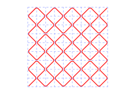
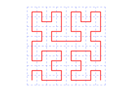
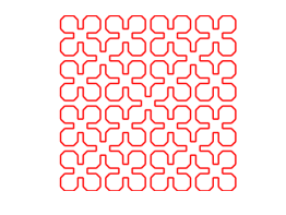
Figure 1. Space-filling curves of Peano, Hilbert and Sierpiński.

Around 1970’s, several remarkable progresses have been made: J. Heighway, a physicist, found the Heighway dragon ([13, 8]); W. Gosper, a computer scientist, found the Gosper island ([13]); H. Lindenmayer, a biologist, introduced L-system ([17]), which becomes a powerful method to produce space-filling curves later.

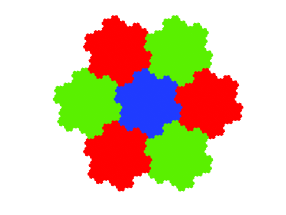
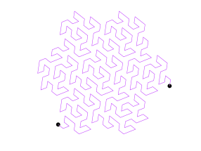
Figure 2. The Gosper island is a 7-reptile, and the Gosper curve is an optimal parametrization.

Two important facts are gradually recognized: All the constructions are based on certain self-similar structures, and certain ‘substitution rules’ play an essential role in the constructions.

Next major progress was made by Dekking [9] (1982), where he claimed that he “introduce a powerful method of describing and generating space-filling curves”. This paper has important impact on both space-filling curves and fractal geometry. On the fractal geometry aspect, [9] leads to the emerge of the notion of graph-directed iterated function system. On the space-filling curve aspect, Dekking’s method has been accepted by computer scientists and as the “vector method”.

In recent years, various interesting constructions of space-filling curves appear on the internet, for example, “www.fractalcurves.com” (see [29]) and “teachout1.net/village/” (see [27]). Besides, space-filling curves of higher dimensional cubes have been studied by Milne [21] and Gilbert [14]. For applications of space-filling curves, see Bader [3] and the references therein.

In this paper and two sequential papers, we unveil the mystery of space-filling curves by providing a rigorous and systematic treatment.

First, let us specify our meaning of space-filling curves. We call an onto mapping from an interval $[a,b]$ to a self-similar set $K$ an optimal parametrization, if it is almost one-to-one, measure-preserving and $1/s$-Hölder continuous, where $s=\dim_{H}K$ is the Hausdorff dimension of $K$. (For precise definition, see Section 2.) It is observed that most classical space-filling curves fulfill the above requirements ([21, 14]), while some others like the Lebesgue curve does not (see Figure 3(right)). It is proper to call an optimal parametrization a space-filling curve if $K$ has non-empty interior, and call it a fractal-filling curve otherwise. However, for simplicity, we shall just call an optimal parametrization a space-filling curve.

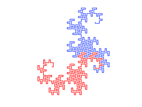
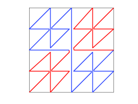
Figure 3. Heighway dragon curve and Lebesgue curve.

The main contribution of this paper is that we introduce a notion of linear GIFS to describe and handle space-filling curves. The graph-directed iterated function system, or GIFS in short, is an important notion in fractal geometry. We equip the functions in a GIFS with a partial order and call it an ordered GIFS, and this order induces a dictionary order of the associated symbolic space. An ordered GIFS is called a linear GIFS, if every two consecutive cylinders have non-empty intersections (see Section 3 for precise definition). We show that

Theorem 1.1.

Let $\{E_{j}\}_{j=1}^{N}$ be the invariant sets of a linear graph-directed IFS satisfying the open set condition and $0<\mathcal{H}^{\delta}(E_{j})<\infty$ for $j=1,\dots,N$, where $\delta$ is the similarity dimension, then $E_{j}$ admits optimal parametrizations for every $j=1,\dots,N$.

The proof of Theorem 1.1 is constructive; hence, to construct space-filling curves is amount to seek a linear GIFS structure of the given set. The common point of the L-language method and Dekking’s vector method is that, first they construct a linear GIFS, and then verify the open set condition.

Remark 1.1.

$(i)$ The notion of linear GIFS can be regarded as a completion of the study of Dekking [9].

$(ii)$ After we finished this paper, we acknowledge that an idea similar to our linear GIFS has appeared in Akiyama and Loridant [1, 2] when studying the parameterizations of boundaries of self-affine tiles.

For an ordered GIFS, one can associate to each invariant set $E_{j}$ a head (the point with the lowest coding) and a tail (the point with the highest coding). Using heads and tails, we define a chain condition (see Section 4) which provides a simple and practical criterion of linear GIFS.

Theorem 1.2.

An ordered GIFS is a linear GIFS if and only if it satisfies the chain condition.

To ‘see’ a space-filling curve, we need to visualize or to approximate a space-filling curve. Using linear GIFS, in Section 6, we give a precise definition of visualizations of a space-filling curve.

To illustrate our theory, we give a brief introduction to the path-on-lattice IFS in Section 5. A nice collection of space-filling curves given by path-on-lattice IFS, many of them are well-known, can be found in the website [29]. A detailed study of the path-on-lattice IFS can be found in [28].

To find the linear GIFS structure of a given self-similar set is a hard question. This question is studied in sequential papers [7] and [23]. We show that

Theorem 1.3.

([7] and [23]) Let $K$ be a connected self-similar set satisfying the open set condition. if $K$ has the finite skeleton property, then it admits optimal parametrizations. In particular, if $K$ satisfies a finite type condition (another important condition in fractal geometry), then it possesses finite skeletons and hence admits optimal parameterizations.

Our theory gives a universal algorithm to find space-filling curves of self-similar set of finite type, that is, as soon as the IFS is given, the computer will do everything. Our study extends almost all the known results on space-filling curves, and shows the internal relation between the space-filling curve and the recent developments of fractal geometry.

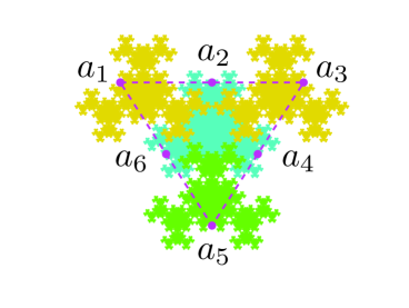
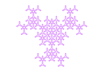
Figure 4. The four-star tile and a space-filling curve.

Example 1.2.

The four-star tile. Pictures in Figure 4 are taking from [27], but there is no explanation how to obtain the space-filling curve. Our study will fill all the gaps from the left picture to the right in Figure 4, which is interesting and highly non-trivial ([7]). A sketch of the approach is provided in Section 7.

The paper is organized as follows. In Section 2, we define optimal parametrization for general compact sets. We introduce the linear GIFS and the chain condition in Section 3 and Section 4, respectively. Section 5 is devoted to the path-on-lattice IFS on the plane. Visualizations of space-filling curves are discussed in Section 6. Section 7 studies the four-star tile. In Section 8, we prove Theorem 1.1, using a measure-recording GIFS.

2. Optimal parameterizations of self-similar sets

Let $K\subset\mathbb{R}^{d}$ be a non-empty compact set. We call $K$ a self-similar set, if it is a union of small copies of itself, precisely, there exist similitudes $S_{1},\dots,S_{N}:\mathbb{R}^{d}\to\mathbb{R}^{d}$ such that

$$K=\bigcup_{j=1}^{N}S_{j}(K).$$

In fractal geometry, the family $\{S_{1},\dots,S_{N}\}$ is called an iterated function system, or IFS in short; $K$ is called the invariant set of the IFS [16, 11]. We denote by ${\mathcal{H}}^{s}$ the $s$-dimensional Hausdorff measure. A set $E\subset\mathbb{R}^{d}$ is called an $s$-set, if $0<{\mathcal{H}}^{s}(E)<\infty$ for some $s\geq 0$.

The IFS $\{S_{1},\dots,S_{N}\}$ is said to satisfy the open set condition (OSC), if there is an open set $U$ such that $\bigcup_{i=1}^{N}S_{i}(U)\subset U$ and the sets $S_{i}(U)$ are disjoint. It is well-known that, if a self-similar set $K$ satisfies the open set condition, then it is an $s$-set. (See [11].)

Remark 2.1.

If an IFS satisfies the OSC condition, and $\dim_{H}K$ equals the space dimension, then $K$ has non-empty interior ([26]), and it is a self-similar tile. Especially, if the contraction ratios of $S_{i}$ are all equal to $r$, then $K$ is called a reptile. (In this case, we must have $r=1/\sqrt[d]{N}$, where $d$ is the dimension of the space.)

Motivated by the studies of the space-filling curves, it is natural to define an optimal parametrization of more general sets (see [6]). Denote ${\mathcal{L}}$ the one-dimensional Lebesgue measure.

Definition 2.2.

Let $K\subset{\mathbb{R}}^{d}$ be an $s$-set. An onto mapping $\psi:[0,1]\rightarrow K$ is called an optimal parametrization of $K$ if the following three conditions are fulfilled.

1. $\psi$ is almost one-to-one, precisely, there exist $K^{\prime}\subset K$ and $I^{\prime}\subset[0,1]$ such that ${\mathcal{H}}^{s}(K\setminus K^{\prime})={\mathcal{L}}([0,1]\setminus I^{\prime})=0$ and $\psi:~{}I^{\prime}\to K^{\prime}$ is a bijection;

2. $\psi$ is measure-preserving in the sense that

   $${\mathcal{H}}^{s}(\psi(F))=c{\mathcal{L}}(F)\text{ and }{\mathcal{L}}(\psi^{-1}(B))=c^{-1}{\mathcal{H}}^{s}(B),$$

   for any Borel set $F\subset[0,1]$ and any Borel set $B\subset K$, where $c={\mathcal{H}}^{s}(K)$.

3. $\psi$ is $1/s$-Hölder continuous, that is, there is a constant $c^{\prime}>0$ such that

   $$|\psi(x)-\psi(y)|\leq c^{\prime}|x-y|^{\frac{1}{s}}\ \text{ for all }x,y\in[0,1].$$

Our main concern is: Does every connected self-similar set admit an optimal parametrization? According to the theorem of Mazurkiewicz-Hahn ([25]), a set is the image of $[0,1]$ under a continuous mapping if and only if it is compact, connected, and locally connected. We note that a connected self-similar set fulfills these conditions, since a self-similar set is locally connected as soon as it is connected ([15]).

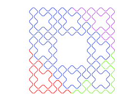
Figure 5. Optimal parameterizations of the Sierpiński gasket and carpet. A detailed study of the carpet is carried out in [7].

For parameterizations of fractal sets, the previous studies focused on the Hölder continuity. de Rham [10], Hata [15] and Remes [24] showed the existence of $1/s$-Hölder continuous parameterizations for certain classes of self-similar sets. Akiyama and Loridant [1, 2] showed the existence when $K$ is the boundary of a class of self-affine tiles (their motivation is to provide an alternative way to show the disk-like property of some planar tiles). Martín and Mattila [19] gave some negative results when $K$ is disconnected.

3. Linear GIFS

In this section, we introduce the notion of linear GIFS.

Let us start with the definition of GIFS. Let $G=(\mathcal{A},\Gamma)$ be a directed graph with vertex set $\mathcal{A}$ and edge set $\Gamma$. Let

$${\mathcal{G}}=\left(g_{\boldsymbol{\gamma}}:\mathbb{R}^{d}\rightarrow\mathbb{R}^{d}\right)_{{\boldsymbol{\gamma}}\in\Gamma}$$

be a family of similitudes. We call the triple $(\mathcal{A},\Gamma,{\mathcal{G}})$, or simply ${\mathcal{G}}$, a graph-directed iterated function system (GIFS). We call $({\mathcal{A}},\Gamma)$ the base graph of the GIFS. Very often but not always, we set ${\mathcal{A}}$ to be $\{1,\dots,N\}$.

Let $\Gamma_{ij}$ be the set of edges from state $i$ to $j$. It is well known that there exist unique non-empty compact sets $\{E_{i}\}_{i=1}^{N}$ satisfying

(3.1) $$E_{i}=\bigcup_{j=1}^{N}\bigcup_{{\boldsymbol{\gamma}}\in\Gamma_{ij}}g_{{\boldsymbol{\gamma}}}(E_{j}),\quad 1\leq i\leq N.$$

We call $\{E_{j}\}_{j=1}^{N}$ the invariant sets of the GIFS ([20][4]).

We say the above GIFS satisfies the open set condition (OSC), if there exist open sets $U_{1},\dots,U_{N}$ such that

$$\bigcup_{j=1}^{N}\bigcup_{\gamma\in\Gamma_{ij}}g_{\gamma}(U_{j})\subset U_{i},\quad 1\leq i\leq N,$$

and the left-hand sides are non-overlapping unions ([20][12]).

Remark 3.1.

It is seen that the set equations (3.1) give all the information of a GIFS, and hence provide an alternative way to define a GIFS. We shall call (3.1) the set equation form of a GIFS.

3.1. Symbolic space related to a graph $G$

Let $G$ be a directed-graph. A sequence of edges in $G$, denoted by ${\boldsymbol{\omega}}=\omega_{1}\omega_{2}\dots\omega_{n}$, is called a path, if the terminate state of $\omega_{i}$ coincides with the initial state of $\omega_{i+1}$ for $1\leq i\leq n-1$. We will use the following notations to specify the sets of finite or infinite paths on $G=(\mathcal{A},\Gamma)$. For $i\in\mathcal{A}$, let

$$\Gamma_{i}^{k},\ \Gamma_{i}^{\ast}\text{ and }\Gamma_{i}^{\infty}$$

be the set of all paths with length $k$, the set of all paths with finite length, and the set of all infinite paths, emanating from the state $i$, respectively. Note that $\Gamma_{i}^{\ast}=\bigcup_{k\geq 1}\Gamma_{i}^{k}$.

For a sequence ${\boldsymbol{\omega}}=(\omega_{k})_{k=1}^{\infty}$, set ${\boldsymbol{\omega}}|_{n}=\omega_{1}\omega_{2}\dots\omega_{n}$ be the prefix of $\omega$ of length $n$. For an infinite path ${\boldsymbol{\omega}}=(\omega_{n})_{n=1}^{\infty}\in\Gamma_{i}^{\infty}$, we call

$$[\omega_{1}\dots\omega_{n}]:=\{{\boldsymbol{\gamma}}\in\Gamma_{i}^{\infty};~{}~{}{\boldsymbol{\gamma}}|_{n}=\omega_{1}\dots\omega_{n}\}$$

the cylinder associated with $\omega_{1}\dots\omega_{n}$.

For a path ${\boldsymbol{\gamma}}=\gamma_{1}\dots\gamma_{n}$, we denote

$$E_{\boldsymbol{\gamma}}:=g_{\gamma_{1}}\circ\cdots\circ g_{\gamma_{n}}(E_{t({\boldsymbol{\gamma}})}),$$

where $t({\boldsymbol{\gamma}})$ denotes the terminate state of the path $\boldsymbol{\gamma}$ (also $\gamma_{n}$). Iterating (3.1) $k$-times, we obtain

(3.2) $$E_{i}=\bigcup_{{\boldsymbol{\gamma}}\in\Gamma_{i}^{k}}E_{\boldsymbol{\gamma}}.$$

We define a projection $\pi:(\Gamma_{1}^{\infty},\dots,\Gamma_{N}^{\infty})\rightarrow(\mathbb{R}^{d},\dots,\mathbb{R}^{d})$, where $\pi_{i}:\Gamma_{i}^{\infty}\rightarrow\mathbb{R}^{d}$ is defined by

(3.3) $$\{\pi_{i}({\boldsymbol{\omega}})\}:=\bigcap_{n\geq 1}E_{\boldsymbol{\omega|_{n}}}.$$

For $x\in E_{i}$, we call ${\boldsymbol{\omega}}$ a coding of $x$ if $\pi_{i}({\boldsymbol{\omega}})=x$. It is folklore that $\pi_{i}(\Gamma_{i}^{\infty})=E_{i}$.

3.2. Order GIFS and linear GIFS

Let $({\mathcal{A}},\Gamma,\mathcal{G})$ be a GIFS. To study the ‘advanced’ connectivity property of the invariant sets, we equip a partial order on the edge set $\Gamma$ enlightened by set equation (3.2). Let $\Gamma_{i}=\Gamma_{i}^{1}$ be the set of edges emanating from the vertex $i$.

Definition 3.2.

We call the quadruple $({\mathcal{A}},\Gamma,\mathcal{G},\prec)$ an ordered GIFS, if $\prec$ is a partial order on $\Gamma$ such that

1. $\prec$ is a linear order when restricted on $\Gamma_{j}$ for every $j\in{\mathcal{A}}$;

2. elements in $\Gamma_{i}\text{ and }\Gamma_{j}$ are not comparable if $i\neq j$.

We denote the edges in $\Gamma_{i}$ by $\gamma_{i,1},\gamma_{i,2},\dots,\gamma_{i,\ell_{i}}$ in an ascending order. For simplicity, we use the following equations to describe an order GIFS (equation form of an ordered GIFS):

$$E_{i}=g_{\gamma_{i,1}}(E_{t(\gamma_{i,1})})+g_{\gamma_{i,2}}(E_{t(\gamma_{i,2})})+\dots+g_{\gamma_{i,\ell_{i}}}(E_{t(\gamma_{i,\ell_{i}})}),\quad i=1,\dots,N,$$

where we use ‘$+$’ instead of ‘$\cup$’ to emphasize the order.

The order $\prec$ induces a dictionary order on each $\Gamma_{i}^{k}$, namely, $\gamma_{1}\gamma_{2}\dots\gamma_{k}\prec\omega_{1}\omega_{2}\dots\omega_{k}$ if and only if $\gamma_{1}\dots\gamma_{\ell-1}=\omega_{1}\dots\omega_{\ell-1}$ and $\gamma_{\ell}\prec\omega_{\ell}$ for some $1\leq\ell\leq k$. Observe that $(\Gamma_{i}^{k},\prec)$ is a linear order. Now we can define the linear GIFS.

Definition 3.3.

Let $({\mathcal{A}},\Gamma,\mathcal{G},\prec)$ be an ordered GIFS with invariant sets $\{E_{i}\}_{i=1}^{N}$. It is termed a linear GIFS, if for all $i\in{\mathcal{A}}$ and $k\geq 1$,

$$E_{\boldsymbol{\gamma}}\cap E_{\boldsymbol{\omega}}\neq\emptyset$$

provided ${\boldsymbol{\gamma}}$ and ${\boldsymbol{\omega}}$ are adjacent paths in $\Gamma_{i}^{k}$.

3.3. Linear IFS

An IFS $\{S_{1},\dots,S_{N}\}$ is a special class of GIFS, where the vertex set is a singleton, and the edge set consists of $N$ self edges which we denote by $1,\dots,N$. The IFS becomes an ordered IFS, if we assume the natural order $1\prec 2\prec\cdots\prec N$.

Remark 3.4.

For an IFS, the associated symbolic space is much simpler. Let $\Sigma=\{1,\dots,N\}$. For $m\geq 1$, we denote $\Sigma^{m}=\{1,2\cdots N\}^{m}$, $\Sigma^{\ast}=\bigcup_{m=0}^{\infty}{\Sigma^{m}}$, and $\Sigma^{\infty}=\{1,2\cdots N\}^{\mathbb{N}}$. For convention, instead of calling $\omega_{1}\dots\omega_{n}\in\Sigma^{n}$ a path, we call it a word. For $i_{1}i_{2}\dots i_{m}\in\Sigma^{*}$, we call $[i_{1}i_{2}\dots i_{m}]=\{{\boldsymbol{\omega}}\in\Sigma^{\infty}~{};~{}~{}{\boldsymbol{\omega}}|_{m}=i_{1}i_{2}\dots i_{m}\}$ a cylinder.

Denote by $K$ the invariant set of the IFS. The projection map $\pi:\Sigma^{\infty}\rightarrow K$ is

$$\{\pi({\boldsymbol{\omega}})\}=\bigcap_{1}^{\infty}S_{{\boldsymbol{\omega}}|_{m}}(K),$$

where $S_{i_{1}i_{2}\dots i_{m}}=S_{i_{1}}\circ S_{i_{2}}\circ\cdots\circ S_{i_{m}}$. We call ${\boldsymbol{\omega}}$ a coding of $x$ if $\pi({\boldsymbol{\omega}})=x$.

Clearly, the von Koch curve is generated by a linear IFS. In Section 5, we shall show that the Peano curve is generated by a linear IFS, while the Heighway dragon and the Hilbert curve are generated by linear GIFS’.

Example 3.5.

Sierpiński curve. Let $T_{1},T_{2},T_{3}$ and $T_{4}$ be a partition of the unit square indicated by Figure 6(right). In Figure 6(left), $T_{j}$, $1\leq j\leq 4$, is divided into $4$ small triangles, where the numbers indicate the order of the small triangles. The four small triangles are images of $T_{j}$ under a map of the form $(x+b)/2$. Hence, we obtain a linear GIFS. Precisely,

$$T_{1}=\frac{T_{1}}{2}+\frac{T_{2}}{2}+\frac{T_{4}+1}{2}+\frac{T_{1}+1}{2}.$$

Similarly equations can be obtained for $T_{2},T_{3}$ and $T_{4}$.

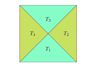
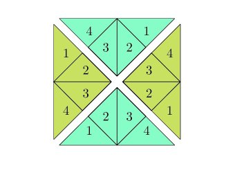
Figure 6. A linear GIFS which generates the Sierpinski curve.

4. The chain condition, proof of Theorem 1.2

Let $(\mathcal{A},\Gamma,{\mathcal{G}},\prec)$ be an ordered GIFS. Denote the invariant sets by $\{E_{i}\}_{i\in{\mathcal{A}}}$. For an edge $\omega\in\Gamma$, recall that $g_{\omega}$ is the associated similitude and $t(\omega)$ is the terminate state.

For $i\in\mathcal{A}$, a path ${\boldsymbol{\omega}}\in\Gamma_{i}^{\infty}$ is called the lowest path, if ${\boldsymbol{\omega}}|_{n}$ is the lowest path in $\Gamma_{i}^{n}$ for all $n$; in this case, we call $a=\pi_{i}({\boldsymbol{\omega}})$ the head of $E_{i}$. Similarly, we define the highest path ${\boldsymbol{\omega}}^{\prime}$ of $\Gamma_{i}^{\infty}$, and we call $b=\pi_{i}({\boldsymbol{\omega}}^{\prime})$ the the tail of $E_{i}$.

Definition 4.1.

An ordered GIFS is said to satisfy the chain condition, if for any $i\in{\mathcal{A}}$, and any two adjacent edges $\omega,\gamma\in\Gamma_{i}$ with $\omega\prec\gamma$,

$$g_{\omega}(\text{tail of }(E_{t(\omega)})=g_{\gamma}(\text{ head of }E_{t(\gamma)}).$$

Clearly, for an ordered IFS $\{S_{1},\dots,S_{N}\}$, the lowest coding is $1^{\infty}$ and the highest coding is $N^{\infty}$. Therefore, the head of $K$ is the fixed point of $S_{1}$, denoted by $Fix(S_{1})$, and the tail of $K$ is $Fix(S_{N})$. Consequently, the chain condition hold if and only if

(4.1) $$S_{i+1}(\text{Fix}(S_{1}))=S_{i}(\text{Fix}(S_{N}))\text{ for }i=1,2,\dots,N-1,$$

Condition (4.1) first appeared in Hata [15], when dealing with the $1/s$-Hölder continuous parametrization of self-similar sets.

Proof of Theorem 1.2..

Suppose $(\mathcal{A},\Gamma,{\mathcal{G}},\prec)$ satisfies the chain condition. Let $i\in\mathcal{A}$, and let ${\boldsymbol{\omega}}$ and ${\boldsymbol{\gamma}}$ be two adjacent paths in $\Gamma_{i}^{n}$ with ${\boldsymbol{\omega}}\prec{\boldsymbol{\gamma}}$. Let ${\boldsymbol{\eta}}={\boldsymbol{\omega}}\wedge{\boldsymbol{\gamma}}$ be the largest common prefix of ${\boldsymbol{\omega}}$ and ${\boldsymbol{\gamma}}$. Then ${\boldsymbol{\omega}}$ and ${\boldsymbol{\gamma}}$ can be written as ${\boldsymbol{\omega}}={\boldsymbol{\eta}}\omega_{k+1}\dots\omega_{n}$ and ${\boldsymbol{\gamma}}={\boldsymbol{\eta}}\gamma_{k+1}\dots\gamma_{n}$. The fact ${\boldsymbol{\omega}}$ and ${\boldsymbol{\gamma}}$ are adjacent implies that

(i) $\omega_{k+1}$ and $\gamma_{k+1}$ are adjacent edges in $\Gamma_{j}$ where $j=t({\boldsymbol{\eta}})$, and $\omega_{k+1}\prec\gamma_{k+1}$;

(ii) $\omega_{k+2}\dots\omega_{n}$ is the highest path in $\Gamma_{t(\omega_{k+1})}^{n-k-1}$ and $\gamma_{k+2}\dots\gamma_{n}$ is the lowest path in $\Gamma_{t(\gamma_{k+1})}^{n-k-1}$.
By item (ii), we have $b=\big{(}\text{tail of }E_{t(\omega_{k+1})}\big{)}\in E_{\omega_{k+2}\dots\omega_{n}}$ since the coding of $b$ is initialled by $\omega_{k+2}\dots\omega_{n}$. Hence

$$g_{\omega_{k+1}}(\text{tail of }E_{t(\omega_{k+1})})\in E_{\omega_{k+1}\dots\omega_{n}}.$$

Similarly,

$$g_{\gamma_{k+1}}(\text{head of }E_{t(\gamma_{k+1})})\in E_{\gamma_{k+1}\dots\gamma_{n}}.$$

Therefore $E_{\omega_{k+1}\dots\omega_{n}}\cap E_{\gamma_{k+1}\dots\gamma_{n}}\neq\emptyset$ by the chain condition. So

$$E_{{\boldsymbol{\omega}}}\cap E_{{\boldsymbol{\gamma}}}=g_{{\boldsymbol{\eta}}}(E_{\omega_{k+1}\dots\omega_{n}}\cap E_{\gamma_{k+1}\dots\gamma_{n}})\neq\emptyset,$$

which proves that the GIFS is linear.

On the other hand, assume that $({\mathcal{A},\Gamma,{\mathcal{G}},\prec})$ is a linear GIFS. Fix $i\in\mathcal{A}$. Let $\omega_{1}$ and $\gamma_{1}$ be adjacent edges in $\Gamma_{i}$ satisfying $\omega_{1}\prec\gamma_{1}$. Let $(\omega_{k})_{k=2}^{\infty}$ be the highest path in $\Gamma_{t(\omega_{1})}^{\infty}$ and $(\gamma_{k})_{k=2}^{\infty}$ be the lowest path in $\Gamma_{t(\gamma_{1})}^{\infty}$. Denote

$${\boldsymbol{\omega}}|_{k}=\omega_{1}\dots\omega_{k}\text{ and }{\boldsymbol{\gamma}}|_{k}=\gamma_{1}\dots\gamma_{k},$$

then for all $k\geq 1$, ${\boldsymbol{\omega}}|_{k}$ and ${\boldsymbol{\gamma}}|_{k}$ are adjacent path in $\Gamma_{i}^{k}$ and so $E_{{\boldsymbol{\omega}}|_{k}}\cap E_{{\boldsymbol{\gamma}}|_{k}}\neq\emptyset$. As we know that

$$g_{\omega_{1}}(\text{tail of }E_{t(\omega_{1})})=\pi_{v}((\omega_{p})_{p\geq 1})\in E_{{\boldsymbol{\omega}}|_{k}},$$

$$g_{\gamma_{1}}(\text{head of }E_{t(\gamma_{1})})=\pi_{v}((\gamma_{p})_{p\geq 1})\in E_{{\boldsymbol{\gamma}}|_{k}}$$

for all $k\geq 1$ , so the distance between $g_{\omega_{1}}(\text{tail of }E_{t(\omega_{1})})$ and $g_{\gamma_{1}}(\text{head of }E_{t(\gamma_{1})})$ can be arbitrarily small. Thus

$$g_{\omega_{1}}(\text{tail of }E_{t(\omega_{1})})=g_{\gamma_{1}}(\text{head of }E_{t(\gamma_{1})}),$$

and the chain condition is verified. The theorem is proved. ∎

Corollary 4.2.

An ordered IFS $\{S_{1},\dots,S_{N}\}$ is a linear IFS if and only if (4.1) holds.

5. Path-on-lattice IFS on the plane

In this section, we study the path-on-lattice IFS on the plane (which we denote by ${\mathbb{C}}$).

Let $\mathbb{L}=\mathbb{Z}+i\mathbb{Z}$ be the square lattice or $\mathbb{L}=\mathbb{Z}+\omega\mathbb{Z}$ be the triangle lattice in the plane, where $\omega=\exp(2\pi i/3)$. We define two points in $\mathbb{L}$ to be neighbors if their distance is $1$. Then we obtain a graph and we still denote it by $\mathbb{L}$.

Let $P$ be a path in $\mathbb{L}$ passing through the points $0=z_{0},z_{1},\dots,z_{n-1},z_{n}=d$ in turn. Let $\Phi=\{\phi_{k}\}_{k=1}^{n}$ be an ordered IFS on $\mathbb{C}$ such that

(5.1) $$\phi_{k}(\{0,d\})=\{z_{k-1},z_{k}\},\text{ for all }k=1,\dots,n.$$

We call such $\Phi$ a path-on-lattice IFS with respect to the path $P$. Clearly the mapping $\phi_{k}$ has the form $\phi_{k}(z)=\alpha z+\beta,\text{ or }\phi_{k}(z)=\alpha\bar{z}+\beta$ with $\alpha,\beta\in{\mathbb{C}}$, and there are four choices of $\phi_{k}$ for each $k$. If we indicate the four mappings by line segments with a half-arrow, then the IFS can be described by a path consisting of marked line segments. If all $\phi_{k}$ are of the form $\alpha z+\beta$, then we say $\Phi$ is reflection-free.

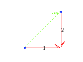
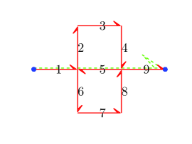
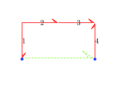
Figure 7. Paths for Heighway dragon curve, Peano curve and Hilbert curve.

Theorem 5.1.

The path-on-lattice IFS is either a linear IFS, or its invariant set can be generated by a linear GIFS with two states. Moreover, the linear GIFS satisfies the OSC if the original IFS does.

Proof.

Let $\{\phi_{k}\}_{k=1}^{n}$ be a path-on-lattice IFS defined by (5.1). Let $K$ be the invariant set.

For $k=1,\dots,n$, define

(5.2) $$v_{k}=\left\{\begin{array}[]{rl}1,&\text{ if }(\phi_{k}(0),\phi_{k}(d))=(z_{k-1},z_{k}),\\ -1,&\text{ if }(\phi_{k}(0),\phi_{k}(d))=(z_{k},z_{k-1}).\end{array}\right.$$

We define an ordered GIFS with two state $\{1,-1\}$ as follows:

(5.3) $$\left\{\begin{array}[]{l}E_{1}=\phi_{1}(E_{v_{1}})+\dots+\phi_{n}(E_{v_{n}}),\\ E_{-1}=\phi_{n}(E_{-v_{n}})+\dots+\phi_{1}(E_{-v_{1}}).\end{array}\right.$$

(One may think that the first equation is corresponding the path $P$, and the second equation is corresponding to the reverse path of $P$.) Clearly $E_{1}=E_{-1}=K$.

We shall show that the head and tail of $E_{1}$ are $0$ and $d$ respectively, and the head and tail of $E_{-1}$ are $d$ and $0$ respectively; then using (5.2), we deduce that the GIFS (5.3) satisfies the chain condition. According to $v_{1}=\pm 1$ and $v_{n}=\pm 1$, we have four choices.

Let us denote the $k$-th edge emanating from $E_{i}$ by $\lambda_{i,k}$. If $v_{1}=1$ and $v_{n}=1$, then the first edge emanating from the vertex $1$ is a self-edge, and hence $(\lambda_{1,1})^{\infty}$ is the lowest coding. It follows that the head of $E_{1}$ is $0$. Similarly, the highest coding emanating from vertex $1$ is $(\lambda_{1,n})^{\infty}$, and so that the tail of $E_{1}$ is $d$. By the same argument, the head of $E_{-1}$ is $d$ and the tail of $E_{-1}$ is $0$.

The other three cases can be proved in the same manner. Moreover, if all $v_{k}$ equal $1$, or all $v_{k}$ equal $-1$, then GIFS (5.3) degenerates to a linear IFS.

As for the open set condition, if the original IFS satisfies the OSC with an open set $U$, then GIFS (5.3) satisfies the OSC with open sets $\{U,U\}$. The theorem is proved. ∎

Remark 5.1.

Algorithms of checking the open set condition of path-on-lattice IFS are discussed in [28]. For the path-on-lattice IFS (5.1), if $n=\|d\|^{2}$ and the OSC holds, then $K$ is a reptile (see Remark 2.1).

Example 5.2.

We give several space-filling curves generated by path-on-lattice IFS’. All of them are reflection-free. The visualizations will be explained in next section.

(1) Heighway dragon. The IFS is given by the path in Figure 7 (left), that is,

$$\phi_{1}(z)=\frac{1-i}{2}z,~{}\phi_{2}(z)=-\frac{1+i}{2}z+(1+i).$$

Denote the Heighway dragon by $H$. By Theorem 5.1, $v_{1}=1,v_{2}=-1$, and $\{H,H\}$ are the invariant sets of the following two-states linear GIFS:

$$\left\{\begin{array}[]{c}E_{1}=\phi_{1}(E_{1})+\phi_{2}(E_{-1})\\ E_{-1}=\phi_{2}(E_{1})+\phi_{1}(E_{-1}),\end{array}\right.$$

(2) Peano curve. The IFS is given by the path in Figure 7(middle). Then $v_{1}=\cdots=v_{9}=1$, and it is a linear IFS: $E=\phi_{1}(E)+\phi_{2}(E)+\cdots+\phi_{9}(E).$

(3) Hilbert curve. The IFS is given by the path in Figure 7(right). Clearly $v_{1}=v_{4}=-1,v_{2}=v_{3}=1$, and the corresponding linear GIFS is:

$$\left\{\begin{array}[]{c}E_{1}=\phi_{1}(E_{-1})+\phi_{2}(E_{1})+\phi_{3}(E_{1})+\phi_{4}(E_{-1})\\ E_{-1}=\phi_{4}(E_{1})+\phi_{3}(E_{-1})+\phi_{2}(E_{-1})+\phi_{1}(E_{1}).\end{array}\right.$$

Example 5.3.

Gosper curve and anti-Gosper curve. The IFS of the Gosper curve is given by the path in Figure 8 (top-left). Clearly $v_{1}=v_{4}=v_{5}=v_{6}=1$, $v_{2}=v_{3}=v_{7}=-1$, and the corresponding linear GIFS can be obtained accordingly.

If we forget the arrows of a path $P$, then we obtain a broken line and we call it the trace of $P$. It is shown in [28] that, among the path-on-lattice IFS’ which are reflection-free and have the same trace as the Gosper curve (there are $128$ of them), none of them satisfies the open set condition except the Gosper curve and anti-Gosper curve. (The path of the anti-Gosper curve is determined by $v_{1}=v_{2}=v_{5}=1$ and $v_{3}=v_{4}=v_{6}=v_{7}=-1$. See Figure 8(bottom).)

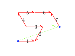
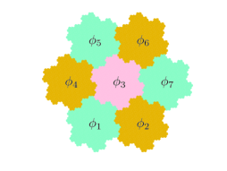
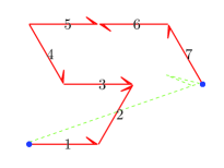
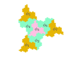
Figure 8. Marked paths for Gosper island and anti-Gosper island.

6. Visualizations of space-filling curves

We consider the visualizations of linear GIFS’ in this section.

Let us start with linear IFS’. Let $\mathcal{S}=\{S_{i}\}_{i=1}^{N}$ be a linear IFS satisfying the open set condition. According to Theorem 1.1, an optimal parametrization $\varphi$ of $K$ can be constructed accordingly. To visualize the limit curve $\varphi$, we need to choose an initial pattern; indeed, the initial pattern can be any curve, but a suitable choice will make the visualization beautiful.

Let us denote by $L_{0}$ the initial pattern, and let $a$ and $b$ be its initial and terminate point, respectively. (Often $L_{0}$ is chosen to be a line segment, which we denote by $\overline{[a,b]}$.)

Fix an $n\geq 1$. For ${\boldsymbol{\omega}}\in\{1,\dots,N\}^{n}$, we denote by $x_{\omega}=S_{\boldsymbol{\omega}}(x)$, and denote ${\boldsymbol{\omega}}^{+}$ the follower of ${\boldsymbol{\omega}}$ (if ${\boldsymbol{\omega}}\neq(N)^{n})$). Connecting $S_{{\boldsymbol{\omega}}}(a)$ and $S_{{\boldsymbol{\omega}}}(b)$ by $S_{{\boldsymbol{\omega}}}(L_{0})$, and connecting $S_{{\boldsymbol{\omega}}}(b)$ and $S_{{\boldsymbol{\omega}}^{+}}(a)$ by a line segment, we obtain the curve

$$L_{n}=\sum_{|{\boldsymbol{\omega}}|=n}\big{(}~{}S_{\boldsymbol{\omega}}(L_{0})+\overline{[b_{{\boldsymbol{\omega}}},a_{{\boldsymbol{\omega}}^{+}}]}~{}\big{)}.$$

Here we use $\sum$ to indicate that $L_{n}$ is the joining of small curves, where the order in given by ${\boldsymbol{\omega}}$. We call $L_{n}$ the $n$-th approximation of the space-filling curve $\varphi$. Different choices of initial patterns may give very different approximations in appearance, though the limit curve is the same.

Example 6.1.

Peano curve. The linear GIFS structure is given in Example 5.2. Figure 9(left and middle) shows two different $2$nd approximations of the Peano curve. For the left picture, the initial pattern $L_{0}=\{3/2\}$ is a singleton, and for the middle picture, $L_{0}=\overline{[\epsilon,3-\epsilon]}$ with $\epsilon=0.4$.

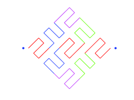
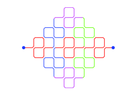
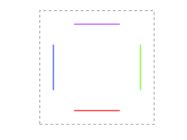
Figure 9. Left and middle: Visualizations of Peano curve. Right: Initial patterns of the Sierpiński curve. The red, green, purple and blue line segments are initial patterns for $T_{1},T_{2},T_{3}$ and $T_{4}$, respectively. The dotted square is the unit square.

As for a linear GIFS, we have to choose an initial pattern for each $E_{j}$, which we denote by $L_{0}^{1},\dots,L_{0}^{N}$. Denote the initial point of the pattern $L_{0}^{j}$ by $a_{j}$ and the end point by $b_{j}$. We define the $n$-th approximation of $E_{j}$ to be

$$L_{n}^{j}=\sum_{{\boldsymbol{\omega}}\in\Gamma_{j}^{n}}\big{(}~{}g_{{\boldsymbol{\omega}}}(L_{0}^{t({\boldsymbol{\omega}})})+\overline{[b_{{\boldsymbol{\omega}}},a_{{\boldsymbol{\omega}}^{+}}]}~{}\big{)},$$

where $b_{{\boldsymbol{\omega}}}=g_{{\boldsymbol{\omega}}}(b_{t({\boldsymbol{\omega}})})$ and $a_{{\boldsymbol{\omega}}^{+}}=g_{{\boldsymbol{\omega}}^{+}}(a_{t({\boldsymbol{\omega}}^{+})})$.

Example 6.2.

For space-filling curves in this example, the linear GIFS structures are given in Example 3.5, 5.2 and 5.3. The visualizations and initial patterns are listed in the following table.

Hilbert curve	Fig. 1(middle)	3rd	$L_{0}^{1}=L_{0}^{2}=\{1+{\mathbf{i}}\}$
Heighway dragon	Fig. 5(left)	8th	$L_{0}^{1}=L_{0}^{2}=\{(1+{\mathbf{i}})/2\}$
Gosper curve	Fig. 2(right)	3rd	$L_{0}^{1}=\overline{[0,d]},L_{0}^{2}=\overline{[d,0]}$ where $d=2+e^{{\mathbf{i}}\pi/3}$
Sierpiński curve	Fig. 1(right)	3rd	Fig. 9(right)

7. The four-star tile

The four-tile star is a $4$-reptile generated by the IFS

$$S_{1}(z)=-\frac{z}{2},\ S_{2}(z)=-\frac{z}{2}-{\mathbf{i}},\ S_{3}(z)=-\frac{z}{2}+\exp({\mathbf{i}}\frac{5\pi}{6}),\ S_{4}(z)=-\frac{z}{2}+\exp({\mathbf{i}}\frac{\pi}{6}).$$

Actually, the $S_{j}$ map the big dotted triangle to the four small triangles in Figure 4. [27] gave a visualization of the four-star tile without any explain (see Figure 4). The mathematical theory behind are provided in [7], and here we give a sketch of it.

7.1. Skeleton

We introduce the notion of skeleton of a self-similar set in [7]. (A skeleton is a kind of vertex set of a fractal.) It is shown that $\{a_{1},\dots,a_{6}\}$ is a skeleton of the four-star tile, where $a_{1}=\frac{4}{3}\exp({\mathbf{i}}\frac{5\pi}{6}),\ a_{2}=\frac{2}{3}{\mathbf{i}},\ a_{3}=\frac{a_{1}}{\omega},\ a_{4}=\frac{a_{2}}{\omega},\ a_{5}=\frac{a_{1}}{\omega^{2}},\ a_{6}=\frac{a_{2}}{\omega^{2}},$ and $\omega=\exp({\mathbf{i}}2\pi/3)$. (See Figure 10 and 11.)

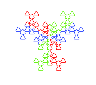
Figure 10. Another visualization of the four-star tile.

7.2. Substitution rule.

Let us consider the polygon $P$ with vertices $a_{1},a_{2},\dots,a_{6}$. Here we regard $P$ as a graph with directed edges, where each edge has the clock-wise orientation. Let us denote the edges by $x,y,z,u,v,w$. (See Figure 11(left).) Figure 11(right) indicates the graph

$$S_{1}(P)\cup S_{2}(P)\cup S_{3}(P)\cup S_{4}(P)$$

which consist of $24$ directed edges. A Eulerian path of the graph is indicated by Figure 11(right), and the path is divided into $6$ parts indicated by different colors.

Replacing a segment in Figure 11(left) by the broken lines in Figure 11(right) with the same color, we obtain a substitution rule.

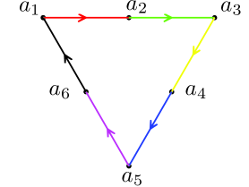
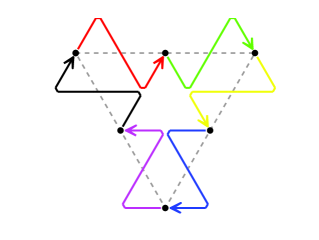
Figure 11. Substitution rule of the Four-star tile

7.3. Linear GIFS.

To precise the meaning of the substitution rule, we introduce the following linear GIFS:

$$\left\{\begin{array}[]{l}X=S_{3}(U)+S_{3}(V)+S_{3}(W)+S_{1}(U),\\ Y=S_{1}(V)+S_{4}(Z)+S_{4}(U)+S_{4}(V),\\ Z=S_{4}(W)+S_{4}(X)+S_{4}(Y)+S_{1}(W),\\ U=S_{1}(X)+S_{2}(V)+S_{2}(W)+S_{2}(X),\\ V=S_{2}(Y)+S_{2}(Z)+S_{2}(U)+S_{1}(Y),\\ W=S_{1}(Z)+S_{3}(X)+S_{3}(Y)+S_{3}(Z).\\ \end{array}\right.$$

It is shown that the four-star tile coincides with $X\cup Y\cup Z\cup U\cup V\cup W$, and it is a non-overlapping union (in Lebesgue measure).

7.4. Visualizations.

Figure 12(left) provides the initial patterns of the third visualization in Figure 4. If we choose the initial patterns in Figure 12(right), we obtain the visualization in Figure 10(right).

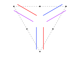
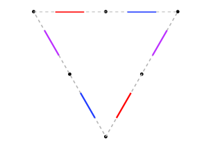
Figure 12. Initial patterns for four-star tile.

8. Proof of Theorem 1.1; Measure-recording GIFS

In this section, we show that the invariant sets of a linear GIFS with the open set condition admit optimal parameterizations. An auxiliary GIFS, called the measure-recording GIFS, will play an important role.

8.1. Preliminaries to dimensions and measures of graph-directed sets

Let $(\mathcal{A},\Gamma,\mathcal{G})$ be the GIFS given by (3.1).

We say a directed-graph $({\mathcal{A}},\Gamma)$ is strongly connected, if there exists a path from $i$ to $j$ for any pair $i,j\in\mathcal{A}$.

Let $r_{e}$ denote the contraction ratio of the similitude $g_{e}$ associated with $e\in\Gamma$. Define a matrix $M(t)$, $t>0$, as

(8.1) $$M(t)=\left(\sum_{e\in\Gamma_{ij}}r_{e}^{t}\right)_{1\leq i,j\leq N}.$$

Then there exists a unique positive number $\delta$ , called the similarity dimension of the GIFS, such that

$$\rho(M(\delta))=1$$

where $\rho(M)$ denotes the spectral radius of a matrix $M$. (See [20], [12].)

Theorem 8.1.

([20]) Let $(\mathcal{A},\Gamma,\mathcal{G})$ be a GIFS satisfying the OSC and let $\delta$ be the similarity dimension. Then

(i) $\dim_{H}E_{i}=\delta$; and $0<H^{\delta}(E_{i})<\infty$ for all $i=1,2,\dots,N$ if $\Gamma$ is strongly connected.

(ii) $(H^{\delta}(E_{1}),\dots,H^{\delta}(E_{N}))^{\prime}$ is an eigenvector of $M(\delta)$ corresponding to eigenvalue $1$.

(iii) ${\mathcal{H}}^{\delta}(E_{\boldsymbol{\omega}}\cap E_{\boldsymbol{\gamma}})=0$ for any incomparable ${\boldsymbol{\omega}},{\boldsymbol{\gamma}}\in\Gamma_{i}^{\ast}$. (Two paths are said to be comparable if one of them is a prefix of the other.)

In the rest of the section, we will always assume that ${\mathcal{G}}$ satisfies the OSC, and that $0<\mathcal{H}^{\delta}(E_{i})<\infty$ for all $i=1,\dots,N$. Let us denote

$$h_{i}={\mathcal{H}}^{\delta}(E_{i})\ \text{ and }\ \mu_{i}={\mathcal{H}}^{\delta}|_{E_{i}},\quad i=1,\dots,N.$$

Now, we define Markov measures on the symbolic spaces $\Gamma_{i}^{\infty}$, $i\in\mathcal{A}$. For an edge $e\in\Gamma$ such that $e\in\Gamma_{ij}$, set

(8.2) $$p_{e}=\frac{h_{j}}{h_{i}}r_{e}^{\delta}.$$

Using Theorem 8.1(ii), it is easy to verify that $(p_{e})_{e\in\Gamma}$ satisfies

(8.3) $$\sum_{j\in{\mathcal{A}}}\sum_{e\in\Gamma_{ij}}p_{e}=1,\text{ for all }i\in\mathcal{A}.$$

We call $(p_{e})_{e\in\Gamma}$ a probability weight vector. Let $\mathbb{P}_{i}$ be a Borel measure on $\Gamma_{i}^{\infty}$ satisfying the relations

(8.4) $$\mathbb{P}_{i}([\omega_{1}\dots\omega_{n}])=h_{i}p_{\omega_{1}}\dots p_{\omega_{n}}$$

for all cylinder $[\omega_{1}\dots\omega_{n}]$. The existence of such measures are guaranteed by (8.3). We call $\{{\mathbb{P}_{i}}\}_{i=1}^{N}$ the Markov measures induced by the GIFS ${\mathcal{G}}$. The following result is folklore, see for instance [20, 18].

Theorem 8.2.

Suppose the GIFS ${\mathcal{G}}$ satisfies the OSC and $0<h_{i}<+\infty$ for all $i$. Let $\pi_{i}:\Gamma_{i}^{\infty}\to E_{i}$ be the projections defined by (3.3). Then

$$\mu_{i}=\mathbb{P}_{i}\circ\pi_{i}^{-1}.$$

8.2. Measure-recording GIFS of a linear GIFS

Let $(\mathcal{A},\Gamma,\mathcal{G},\prec)$ be a linear GIFS such that the open set condition is fulfilled and $0<h_{i}={\mathcal{H}}^{\delta}(E_{i})<\infty$ for all $i$. Set

$$F_{i}=[0,h_{i}],\quad i=1,\dots,N.$$

Fix a state $i$. We list the edges in $\Gamma_{i}$ in the ascendent order with respect to $\prec$:

$$\gamma_{1},\dots,\gamma_{\ell_{i}}.$$

Recall that $t(\gamma)$ denotes the terminate state of an edge $\gamma$. Then according to the set equation form of ${\mathcal{G}}$, $E_{i}$ can be written as

$$E_{i}=g_{\gamma_{1}}(E_{t(\gamma_{1})})+\cdots+g_{\gamma_{\ell_{i}}}(E_{t(\gamma_{\ell_{i}})}).$$

Let

$$f_{\gamma_{k}}(x)=r_{\gamma_{k}}^{\delta}x+b_{k}:~{}~{}\mathbb{R}\longrightarrow\mathbb{R},\quad 1\leq k\leq\ell_{i}$$

be similitudes such that

(8.5) $$F_{i}=f_{\gamma_{1}}(F_{t(\gamma_{1})})+\cdots+f_{\gamma_{\ell_{i}}}(F_{t(\gamma_{\ell_{i}})})$$

where the right hand side is a non-overlapping union of consecutive intervals from left to right. Indeed, we must have $b_{k}=\sum_{j=1}^{k-1}h_{t(\gamma_{j})}r_{\gamma_{j}}^{\delta}$, and (8.5) holds by equation (8.3). Doing this for all $i\in{\mathcal{A}}$, then (8.5) give us an ordered GIFS with the natural order. We denote this GIFS by

$$(\mathcal{A},\Gamma,{\mathcal{G}}^{*},\prec),$$

and call it the measure-recording GIFS of $({\mathcal{A}},\Gamma,{\mathcal{G}},\prec)$.

Clearly, the measure-recording GIFS inherits the graph structure and the order structure of the original GIFS; moreover, it records the Hausdorff measure information of the original GIFS. The following facts are obvious.

• $\{F_{i}\}_{i=1}^{N}$ are the invariant sets of the measure-recording GIFS.

• For an edge $e\in\Gamma$, the contraction ratio of $f_{e}$ is $r_{e}^{\delta}$, and the similarity dimension $\delta^{*}$ of ${\mathcal{G}}^{*}$ is $1$.

• ${\mathcal{G}}^{*}$ satisfies the OSC.

• The measure-recording GIFS shares the same symbolic spaces with the original GIFS.

Let

$$\pi_{i}:\Gamma_{i}^{\infty}\rightarrow E_{i}\text{ and }\rho_{i}:\Gamma_{i}^{\infty}\rightarrow F_{i},\quad i=1,\dots,N,$$

be projections w.r.t. the GIFS $({\mathcal{G}})$ and $({\mathcal{G}}^{*})$, respectively. (See (3.3).) Then

Lemma 8.1.

The Markov measure induced by the measure-recording GIFS coincides with that induced by the original GIFS.

Proof.

Let $(p_{e})_{e\in\Gamma}$ and $(p_{e}^{*})_{e\in\Gamma}$ be the probability weights corresponding to ${\mathcal{G}}$ and ${\mathcal{G}}^{*}$, respectively. Since

$$p_{e}=\frac{h_{j}}{h_{i}}(r_{e})^{\delta}=\frac{\mathcal{L}(F_{j})}{\mathcal{L}(F_{i})}(r_{e}^{\delta})^{\delta^{*}}=p_{e}^{*},$$

the two systems define the same probability weight vector and hence define the same Markov measure. ∎

Define

(8.6) $$\psi_{i}:=\pi_{i}\circ\rho_{i}^{-1}.$$

The following lemma verifies that $\psi_{i}$ is a well-defined mapping from $F_{i}$ to $E_{i}$.

Lemma 8.2.

Suppose $x\in F_{i}$ has two $\rho_{i}$-codings, say $\rho_{i}^{-1}(x)=\{{\boldsymbol{\omega}},{\boldsymbol{\gamma}}\}.$ Then

$$\pi_{i}({\boldsymbol{\omega}})=\pi_{i}({\boldsymbol{\gamma}}).$$

Proof.

Write ${\boldsymbol{\omega}}=(\omega_{k})_{k=1}^{\infty}$ and ${\boldsymbol{\gamma}}=(\gamma_{k})_{k=1}^{\infty}$. We claim that $\omega_{1}\dots\omega_{n}$ and $\gamma_{1}\dots\gamma_{n}$ are adjacent for all $n\geq 1$, for otherwise, there exists $\eta_{1}\dots\eta_{n}$ such that

$$\omega_{1}\dots\omega_{n}\prec\eta_{1}\dots\eta_{n}\prec\gamma_{1}\dots\gamma_{n},$$

and the interval $F_{\eta_{1}\dots\eta_{n}}$ separates $F_{\omega_{1}\dots\omega_{n}}$ and $F_{\gamma_{1}\dots\gamma_{n}}$, contradicting to $\rho_{i}({\boldsymbol{\omega}})=\rho_{i}({\boldsymbol{\gamma}})=x$. Our claim is proved. It follows that $E_{\omega_{1}\dots\omega_{n}}\cap E_{\gamma_{1}\dots\gamma_{n}}\neq\emptyset$, since $(\mathcal{A},\Gamma,\mathcal{G},\prec)$ is a linear GIFS. Hence $|\pi_{i}({\boldsymbol{\omega}})-\pi_{i}({\boldsymbol{\gamma}})|\leq\text{diam }E_{{\boldsymbol{\omega}}|_{n}}+\text{diam }E_{{\boldsymbol{\gamma}}|_{n}}$, so the distance between $\pi_{i}({\boldsymbol{\omega}})$ and $\pi_{i}({\boldsymbol{\gamma}})$ can be arbitrarily small, which implies that $\pi_{i}({\boldsymbol{\omega}})=\pi_{i}({\boldsymbol{\gamma}})$. ∎

Now, we prove Theorem 1.1 by showing that the mapping $\psi_{i}$ is an optimal parametrization of $E_{i}$.

8.3. Proof of Theorem 1.1.

Let ${\mathcal{G}}^{*}$ be the measure-recording GIFS of ${\mathcal{G}}$. Let $\psi_{i}=\pi_{i}\circ\rho_{i}^{-1}.$ Let $\nu_{i}={\mathcal{L}}|_{F_{i}}$ be the restriction of the Lebesgue measure on $F_{i}$, $\mu_{i}={\mathcal{H}}^{s}|_{E_{i}}$, and ${\mathbb{P}}_{i}$ be the common Markov measure of ${\mathcal{G}}$ and ${\mathcal{G}}^{*}$. Then $\nu_{i}=\mathbb{P}_{i}\circ\rho_{i}^{-1}$, $\mu_{i}=\mathbb{P}_{i}\circ\pi_{i}^{-1}$ by Theorem 8.2.

(i) First, we prove that $\psi_{i}$ is almost one to one.

Let $Q_{i}$ be the set of points in $E_{i}$ possessing more than one $\pi_{i}$-codings. Since

$$Q_{i}=\bigcup_{n\geq 1}\bigcup_{{{\boldsymbol{\gamma}}\neq{\boldsymbol{\omega}}\in\Gamma_{i}^{n}}}E_{\boldsymbol{\gamma}}\cap E_{\boldsymbol{\omega}},$$

and $\mu_{i}(E_{{\boldsymbol{\gamma}}}\cap E_{{\boldsymbol{\omega}}})=0$ by Theorem 8.1(iii), we obtain $\mu_{i}(Q_{i})=0$. Denote

$$\Delta_{i}=\pi_{i}^{-1}(Q_{i}),$$

then $\pi_{i}$ is injective when restricted to $\Gamma_{i}^{\infty}\setminus\Delta_{i}$, and ${\mathbb{P}}_{i}(\Delta_{i})=\mu_{i}(Q_{i})=0$.

Similarly, let $Q_{i}^{\prime}$ be the set of points in $F_{i}$ possessing more than one $\rho_{i}$-codings, then $\nu_{i}(Q_{i}^{\prime})=0$. Let $\Delta_{i}^{\prime}=\rho_{i}^{-1}(Q_{i}^{\prime})$, then $\rho_{i}$ is injective when restricted to $\Gamma_{i}^{\infty}\setminus\Delta_{i}^{\prime}$, and ${\mathbb{P}}_{i}(\Delta_{i}^{\prime})=\nu_{i}(Q_{i}^{\prime})=0$.

Let

$$F_{i}^{\prime}=\rho_{i}(\Gamma_{i}^{\infty}\setminus(\Delta_{i}\cup\Delta_{i}^{\prime})),\quad E_{i}^{\prime}=\pi_{i}(\Gamma_{i}^{\infty}\setminus(\Delta_{i}\cup\Delta_{i}^{\prime})),$$

Then $\psi_{i}:F_{i}^{\prime}\to E_{i}^{\prime}$ is one-to-one, $\nu_{i}(F_{i}\setminus F_{i}^{\prime})\leq\mathbb{P}_{i}(\Delta_{i}\cup\Delta_{i}^{\prime})=0$, and $\mu_{i}(E_{i}\setminus E_{i}^{\prime})\leq\mathbb{P}_{i}(\Delta_{i}\cup\Delta_{i}^{\prime})=0$.

(ii) Secondly, we prove that $\psi_{i}$ is measure-preserving. For any Borel set $B\subset\mathbb{R}^{d}$, we need to show that $\nu_{i}(\psi_{i}^{-1}(B))=\mu_{i}(B)$; due to (i), it suffices to show this hold for $B\subset E_{i}^{\prime}$. Indeed, for $B\subset E_{i}^{\prime}$, we have

$$\nu_{i}(\psi_{i}^{-1}(B))=\nu_{i}(\rho_{i}\circ\pi_{i}^{-1}(B))=\mathbb{P}_{i}\circ\rho_{i}^{-1}\circ\rho_{i}\circ\pi_{i}^{-1}(B)=\mathbb{P}_{i}\circ\pi_{i}^{-1}(B)=\mu_{i}(B),$$

where the third equality holds since $\rho_{i}$ is a bijection when restricted to $(\Gamma_{i}^{\infty}\setminus(\Delta_{i}\cup\Delta_{i}^{\prime}))$. Similarly, for any Borel set $B\subset\mathbb{R}$, one can show that $\mu_{i}(\psi_{i}(B))=\nu_{i}(B).$

(iii) Finally, we prove the $1/\delta$-Hölder continuity of $\psi_{i}$.

Let $x_{1},x_{2}$ be two points in $F_{i}=[0,h_{i}]$. Let $k$ be the smallest integer such that $x_{1},x_{2}$ belong to two different cylinders of rank $k$, say, $x_{1}\in\rho_{i}([{\boldsymbol{\omega}}])$, $x_{2}\in\rho_{i}([{\boldsymbol{\gamma}}])$, where ${\boldsymbol{\omega}}\neq{\boldsymbol{\gamma}}\in\Gamma_{i}^{k}$. It is seen that ${\boldsymbol{\omega}}=\omega_{1}\dots\omega_{k}$ and ${\boldsymbol{\gamma}}$ differ only at the last edge, that is,

$${\boldsymbol{\gamma}}=\omega_{1}\dots\omega_{k-1}\gamma_{k}.$$

We consider two cases according to ${\boldsymbol{\omega}}$ and ${\boldsymbol{\gamma}}$ are adjacent or not.

Case 1.   ${\boldsymbol{\omega}}$ and ${\boldsymbol{\gamma}}$ are not adjacent. (See figure 13.)

Figure 13. ${{\boldsymbol{\omega}}}$ and ${{\boldsymbol{\gamma}}}$ are not adjacent

Then there is a cylinder ${\boldsymbol{\eta}}=\omega_{1}\dots\omega_{k-1}\eta_{k}$ between ${\boldsymbol{\omega}}$ and ${\boldsymbol{\gamma}}$, so

$$|x_{1}-x_{2}|\geq\text{diam}~{}F_{\boldsymbol{\eta}}\geq h\cdot r_{{\boldsymbol{\eta}}}^{\delta}\geq h\cdot r_{{\boldsymbol{\omega}}^{*}}^{\delta}\cdot r_{\min}^{\delta},$$

where ${\boldsymbol{\omega}}^{*}=\omega_{1}\dots\omega_{k-1}$ is the path obtained by deleting the last edge in ${\boldsymbol{\omega}}$, and

$$h=\min\{h_{i};~{}i=1,\dots,N\},\quad r_{\min}=\min\{r_{e};~{}e\in\Gamma\}.$$

Since $x_{1},x_{2}$ belong to $\rho_{i}([{\boldsymbol{\omega}}^{*}])$, the images of $x_{1}$ and $x_{2}$ under $\pi_{i}\circ\rho_{i}^{-1}$, which we denote by $y_{1}$ and $y_{2}$ respectively, belong to $\pi_{i}([{\boldsymbol{\omega}}^{*}])=E_{{\boldsymbol{\omega}}^{*}}$. It follows that

(8.7) $$|y_{1}-y_{2}|\leq\text{diam }E_{{\boldsymbol{\omega}}^{*}}\leq D\cdot r_{{\boldsymbol{\omega}}^{*}}\leq D\cdot r_{\min}^{-1}\cdot h^{-1/\delta}\cdot|x_{1}-x_{2}|^{1/\delta},$$

where

$$D=\max_{1\leq i\leq N}\text{ diam }E_{i}.$$

Case 2.   ${\boldsymbol{\omega}}$ and ${\boldsymbol{\gamma}}$ are adjacent. (See figure 14(left).)

Figure 14. ${{\boldsymbol{\omega}}}$ and ${{\boldsymbol{\gamma}}}$ are adjacent

Let $x_{3}$ be the intersection of $F_{\boldsymbol{\omega}}$ and $F_{\boldsymbol{\gamma}}$. Let $k^{\prime}$ be the smallest integer such that $x_{1}$ and $x_{3}$ belong to different cylinders of rank $k^{\prime}$, say, $x_{1}\in\rho_{i}([{\boldsymbol{\omega}}^{\prime}])$ and $x_{3}\in\rho_{i}([{\boldsymbol{\omega}}^{\prime\prime}])$ (see Figure 14(right)), then $|x_{1}-x_{3}|\geq\text{diam}~{}F_{{\boldsymbol{\omega}}^{\prime\prime}}$ since $x_{3}$ is an endpoint.

Let $y_{3}=\psi_{i}(x_{3})$. Similar to Case 1, we have

$$|y_{1}-y_{3}|\leq D\cdot r_{\min}^{-1}\cdot h^{-1/\delta}\cdot|x_{1}-x_{3}|^{1/\delta}.$$

By the same argument, we have

$$|y_{2}-y_{3}|\leq D\cdot r_{\min}^{-1}\cdot h^{-1/\delta}\cdot|x_{2}-x_{3}|^{1/\delta}.$$

Hence, by the fact $x_{3}$ locates between $x_{1}$ and $x_{2}$,

(8.8) $$|y_{1}-y_{2}|\leq 2D\cdot r_{\min}^{-1}\cdot h^{-1/\delta}\cdot|x_{1}-x_{2}|^{1/\delta}.$$

Therefore, (8.7) and (8.8) verify the $1/\delta$- Hölder continuity of $\psi_{i}$. $\Box$

Remark 8.3.

We note that the initial point $\psi_{i}(0)$ is the head of $E_{i}$, and the terminate point $\psi_{i}(h_{i})$ is the tail of $E_{i}$.

Remark 8.4.

In some text books, the space-filling curves is concerned; for example, ‘Real Analysis’ by Stein and Shakarchi (2005), ‘Topology’ by Munkres (2000), ‘Basic Topology’ by Armstrong (1997). The above proof extends the arguments in these books.

References

- [1] S. Akiyama and B. Loridant: Boundary parametrization of planar self-affine tiles with collinear digit set, Sci. China Math., 53 (2010), 2173–2194.
- [2] S. Akiyama and B. Loridant: Boundary parametrization of self-affine tiles, J. Math. Soc. Japan, 63 (2011), no. 2, 525–579.
- [3] M. Bader: Space-filling curves. An introduction with applications in scientific computing. Texts in Computational Science and Engineering, 9. Springer, Heidelberg, 2013.
- [4] T. Bedford: Dimension and dynamics of fractal recurrent sets, J. London Math. Soc.(2), 33 (1986) 89–100.
- [5] D. Ciesielska: On the 100 anniversary of the Sierpiński space-filling curve, Wiadomoci Matematyczne 48 (2012), no. 2, 69.
- [6] X. R. Dai and Y. Wang: Peano curves on connected self-similar sets, Unpublished note (2010).
- [7] X. R. Dai, H. Rao and S. Q. Zhang: Space-filling curves of self-similar sets (II): Finite skeleton, Eulerian path and substitution rule. Preprint 2015.
- [8] C. Davis and D. E. Knuth: Number representations and dragon curves I, II, Recreational Math. 3 (1970), 66–81 and 133–149.
- [9] F. M. Dekking: Recurrent sets, Adv. in Math., 44 (1982), no. 1, 78–104.
- [10] G. de Rham: Sur quelques courbes définies par des équations fonctionnelles, Rend. Sem. Mat. Torino, 16 (1957), 101–113.
- [11] K. J. Falconer: Fractal Geometry, Mathematical Foundations and Applications, Wiley, New York, 1990.
- [12] K. J. Falconer: Techniques in fractal geometry, John Wiley & Sons, Ltd., Chichester, 1997.
- [13] M. Gardner: In which “monster” curves force redefinitions of the word “curve”, Scientific American, 235 (1976), 124–133.
- [14] W. J. Gilbert: A cube-filling Hilbert curve, Mathematical Intelligencer, 6 (1984), no. 3, 78.
- [15] M. Hata: On the structure of self-similar sets, Japan J. Appl. Math., 2 (1985), 381–414.
- [16] J. E. Hutchinson: Fractal and self similarity, Indian Univ. Math. J., 30 (1981), 713–747.
- [17] A. Lindenmayer: Mathematical models for cellular interacton in development, Parts I and II, Journal of Theoretical Bilology, 30 (1968), 280–315.
- [18] J. Luo and Y. M. Yang: On single-matrix graph-directed iterated function systems, J. Math. Anal. Appl., 372 (2010), no. 1, 8–18.
- [19] M. A. Martín and P. Mattila: On the parametrizations of self-similar and other fractal sets, Trans. Amer. Soc., 128 (2000), 2641–2648.
- [20] D. Mauldin and S. Williams: Hausdorff dimension in graph directed constructions, Trans. Amer. Math. Soc., 309 (1988), 811–829.
- [21] S. C. Milne: Peano curves and smoothness of functions, Adv. Math., 35 (1980), 129–157.
- [22] G. Peano: Sur une courbe qui remplit toute une aire plane, Math. Ann., 36 (1890), 157–160.
- [23] H. Rao and S. Q. Zhang: Space-filling curves of self-similar sets (III): Primitive and consistency. Preprint 2015.
- [24] M. Remes: Hölder parametrizations of self-similar sets, Ann. Acad. Sci. Fenn. Math. Diss., no. 112, (1998), 68 pp.
- [25] H. Sagan: Space-Filling Curve, Springer-Verlag, New York, 1994.
- [26] A. Schief: Separation properties for self-similar sets, Proc. Amer. Math. Soc., 122 (1994), 114–115.
- [27] G. Teachout: Spacefilling curve designs featured in the web site: http://teachout1.net/village/.
- [28] Y.M. Yang and S. Q. Zhang, Path-on-lattice IFS and space-filling curves. Preprint 2015.
- [29] J. Ventrella: Fractal Curves in the web site :http://www.fractalcurves.com/.