Uncertainties in Galactic Chemical Evolution Models

Abstract

We use a simple one-zone galactic chemical evolution model to quantify the uncertainties generated by the input parameters in numerical predictions for a galaxy with properties similar to those of the Milky Way. We compiled several studies from the literature to gather the current constraints for our simulations regarding the typical value and uncertainty of the following seven basic parameters: the lower and upper mass limits of the stellar initial mass function (IMF), the slope of the high-mass end of the stellar IMF, the slope of the delay-time distribution function of Type Ia supernovae (SNe Ia), the number of SNe Ia per M_⊙ formed, the total stellar mass formed, and the final mass of gas. We derived a probability distribution function to express the range of likely values for every parameter, which were then included in a Monte Carlo code to run several hundred simulations with randomly selected input parameters. This approach enables us to analyze the predicted chemical evolution of 16 elements in a statistical manner by identifying the most probable solutions along with their 68 % and 95 % confidence levels. Our results show that the overall uncertainties are shaped by several input parameters that individually contribute at different metallicities, and thus at different galactic ages. The level of uncertainty then depends on the metallicity and is different from one element to another. Among the seven input parameters considered in this work, the slope of the IMF and the number of SNe Ia are currently the two main sources of uncertainty. The thicknesses of the uncertainty bands bounded by the 68 % and 95 % confidence levels are generally within 0.3 and 0.6 dex, respectively. When looking at the evolution of individual elements as a function of galactic age instead of metallicity, those same thicknesses range from 0.1 to 0.6 dex for the 68 % confidence levels and from 0.3 to 1.0 dex for the 95 % confidence levels. The uncertainty in our chemical evolution model does not include uncertainties relating to stellar yields, star formation and merger histories, and modeling assumptions.

1. Introduction

Numerical simulations in astrophysics are challenging because of their multi-scale nature. In principle, galactic chemical evolution models need to resolve both the evolution of stars and the evolution of galaxies. In practice, this is problematic because stellar evolution implies timescales as low as a few seconds in advanced burning stages, while galaxies have lifetimes that spread over billions of years. In addition, stars occupy an insignificant fraction of the volume of a galaxy, which is a concern for hydrodynamic simulations. Of course, it is not possible to resolve all of these different scales with the computational power currently available. In order to consistently follow the chemical evolution of a galaxy, simulations need to incorporate subgrid treatments to include the physics that cannot be spatially or temporarily resolved. This is done by using the previously calculated outputs of other simulations that fully focus on the unresolved problem (e.g., stellar evolution), or by using simplified analytical models.

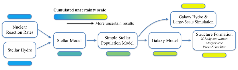
Figure 1.— Growth of uncertainties in chemical evolution studies from stellar to cosmological scales. This diagram only serves as a qualitative visualization and may not be complete.

Stellar models represent the building blocks of chemical evolution models by providing, in the form of yield tables, the mass ejected by stars for different elements and metallicities (e.g., Portinari et al. 1998; Iwamoto et al. 1999; Chieffi & Limongi 2004; Travaglio et al. 2004; Meynet & Maeder 2005; Nomoto et al. 2006; Heger & Woosley 2010; Karakas 2010; Pignatari et al. 2013a). These stellar yields are then converted into simple stellar populations (SSPs) by using stellar lifetimes and an initial mass function (IMF). In this context, an SSP refers to a mass element that is converted into stars according to a presented star formation rate. In hydrodynamical simulations, SSP units are used to inject mass locally around individual star particles (e.g., Oppenheimer & Davé 2008; Wiersma et al. 2009; Hopkins et al. 2012; Brook et al. 2014). This procedure can be applied on galactic and cosmological scales. In semi-analytical models, SSP units are combined together to inject mass in the gas reservoirs of a galaxy (e.g., Benson & Bower 2010; Tumlinson 2010; Crosby et al. 2013; Yates et al. 2013; De Lucia et al. 2014; Gómez et al. 2014; Côté et al. 2015). Usually, these models can be used in a cosmological context by combining them with N-body simulations and merger trees.

Chemical evolution studies can also be applied to the circumgalactic, intergalactic, and intracluster medium. Galactic outflows, gas stripping, and galaxy disruptions are responsible for entraining enriched material beyond the galactic scale (see Martel et al. 2012; Benítez-Llambay et al. 2013; Shen et al. 2013). From the production of the elements in stars to the enrichment of intergalactic gas, there is a chain of models integrated with each other. Stellar models are actually not the starting point of this chain – they depend on nuclear physics for defining the production of new elements in stellar interiors (e.g., Wiescher et al. 2012) and on hydrodynamic experiments and simulations for constraining the behavior of gas experiencing phenomena such as turbulence and mixing (e.g., Meakin & Arnett 2007; Woodward et al. 2008, 2015; Arnett et al. 2010; Herwig et al. 2014; Smith & Arnett 2014) or exposed to more extreme conditions during supernova explosions (e.g., Janka et al. 2012; Burrows 2013; Hix et al. 2014; Wongwathanarat et al. 2015).

Although this chain of models offers a very efficient way to create solid links between different scales despite the limitation of current computational resources, it is critical to acknowledge that a great deal of uncertainty is attached to the numerical predictions coming out of this chain, particularly at galactic and cosmological scales. At every scale, each model deals with their own sets of assumptions and uncertainties. Each time a model in the chain uses the results of the models that precede it, it ends up implicitly including the uncertainties of these preceding models (Figure 1). In that sense, chemical evolution studies may already hide potential uncertainties beyond observational errors. In order to move toward a better quantification of the global level of uncertainty pertaining to chemical evolution modeling, it is important to establish the uncertainties at every step along the chain. In this paper, we focus on the SSP and galactic levels, as a critical component of this bigger picture between nuclear astrophysics and cosmology simulations.

As clearly demonstrated by Romano et al. (2010), the choice of stellar yields is a major source of uncertainty in galactic chemical evolution models (see also Gibson 1997, 2002; Wiersma et al. 2009; Mollá et al. 2015). In addition, all of those yields are affected by nuclear reaction rate uncertainties (e.g., Rauscher et al. 2002; El Eid 2004; Herwig et al. 2006; Tur et al. 2007, 2009, 2010; Pignatari et al. 2010, 2013b; Iliadis et al. 2011; Wiescher et al. 2012; Parikh et al. 2013; Travaglio et al. 2014) and by stellar modeling assumptions (e.g., Woosley et al. 2002; Hirschi et al. 2005; Karakas 2014; Karakas & Lattanzio 2014; Jones et al. 2015; Lattanzio et al. 2015).

Another source of uncertainty is the input parameters associated with SSPs. Romano et al. (2005) studied the impact of the IMF (see also Mollá et al. 2015) and the stellar lifetimes, while Matteucci et al. (2009), Wiersma et al. (2009), and Yates et al. (2013) explored the impact of the delay-time distribution (DTD) function used to calculate the rate of Type Ia supernovae (SNe Ia). However, all of these studies focused on the uncertainties resulting from the different options offered in the literature, and not on the uncertainties in the measurements that were used to constrain the input parameters in the first place.

The goal of the present paper is to complement the work discussed above by using the simplest possible model – a closed-box, single-zone model – and by exploring the impact of the uncertainties associated with a range of input parameters corresponding to the measurements of several observationally estimated quantities relating to the stellar IMF, to SNe Ia properties, and to the global properties of the Milky Way galaxy. We do not claim that a closed-box model is representative of the Milky Way, which is why we do not compare our results with observational data in this paper. We are only using the Galaxy as a test case to constrain the uncertainty of some of our input parameters in order to understand how they affect our predictions. More realistic chemical evolution models designed to reproduce the Milky Way can be found in the literature (e.g., Chiappini et al. 2001; Kobayashi et al. 2011; Minchev et al. 2013; Mollá et al. 2015; Shen et al. 2015; van de Voort et al. 2015; Wehmeyer et al. 2015).

Our aim in this work is to place lower bounds on the uncertainties in predictions relating to some of the most fundamental input parameters in all chemical evolution models. In future papers, we will expand our approach to include galactic inflows and outflows, variable star formation rates, the effect of mergers and environment, and varied stellar evolution models and nuclear physics input. Ultimately, our goal is to obtain a quantification of uncertainty in chemical evolution modeling. It will be useful to develop intuition about what types of predictions from modern chemical evolution models are reliable when compared to modern observational data sets. Furthermore, realistic uncertainties will be critical when comparing these models to modern stellar surveys using statistical techniques such as Bayesian Markov Chain Monte Carlo (e.g., Gómez et al. 2012, 2014; Gelman 2014). Galactic chemical evolution models are an important tool for probing stellar models. This requires that we know how reliable the chemical evolution models are.

This paper is organized as follows. In Section 2, we briefly describe our galactic chemical evolution code and our choice of stellar yields. We describe, in Section 3, the seven input parameters varied in our code and present compilations of the different studies used to constrain them. The probability distribution function (PDF), the average value, and the uncertainty of each parameter are calculated in Section 4. We present in Section 5 the overall uncertainties in the chemical evolution of 16 elements, along with the individual contribution of each parameter. We discuss some caveats and limitations relating to our results in Section 6. Finally, our conclusions are given in Section 7.

2. Chemical Evolution Code

In this paper, we use the SYGMA module (C. Ritter et al. in preparation), which stands for Stellar Yields for Galactic Modeling Applications, to calculate the composition of the stellar ejecta coming out of SSP units as a function of time and metallicity using a set of stellar yields. We also use a simplified version of the OMEGA module (Côté et al. 2016), which stands for One-zone Model for the Evolution of GAlaxies, to combine the contribution of several SSPs to calculate the chemical evolution of a gas reservoir. These python codes are part of an upcoming numerical pipeline designed to create permanent connections between nuclear physics, stellar evolution, and galaxy evolution. These modules will ultimately be used to probe the impact of nuclear physics and stellar modeling assumptions on galactic chemical evolution, but will also provide input data for simulations aiming to study chemical evolution in a cosmological context.

2.1. Closed Box Model

The presented version of OMEGA is a classical one-zone, closed-box galaxy model (see Talbot & Arnett 1971) with a continuous star formation history (SFH) where stars form and inject new elements within the same gas reservoir, using SYGMA to create an SSP at every timestep. Single-zone, closed-box models solve the following equation at each timestep during a simulation (e.g., Pagel 2009):

$$M_{\rm gas}(t+\Delta t)=M_{\rm gas}(t)+\Big{[}\dot{M}_{\rm ej}(t)-\dot{M}_{\star}(t)\Big{]}\Delta t,$$ (1)

where, $M_{\rm gas}(t)$ and $\Delta t$ are, respectively, the mass of the gas reservoir at time $t$, and the duration of the timestep. $\dot{M}_{\rm ej}(t)$ and $\dot{M}_{\star}(t)$ are the stellar mass loss rate and the star formation rate. In this paper, we ignore the contribution of galactic inflows and outflows. As mentioned in Section 1, our goal is not to present a sophisticated chemical evolution code, but rather to focus on the impact of basic input parameters on numerical predictions.

We use a set of stellar yields to calculate the mass ejected by stars (see Section 2.2), and accordingly the chemical composition of the gas reservoir is known at any time $t$. When gas is converted into stars to form an SSP, the mass of each element locked away is calculated following the current chemical composition of the gas reservoir. The metallicity of an SSP formed at time $t$ is then represented by the gas metallicity at that time, which is given by

$$Z_{\mathrm{gas}}(t)=\frac{M_{\mathrm{gas}}(t)-M_{\mathrm{H}}(t)-M_{\mathrm{He}}(t)}{M_{\mathrm{gas}}(t)}.$$ (2)

At each timestep, the total stellar ejecta is calculated by considering the mass $M$, the metallicity $Z$, and the age $\tau$ of every individual SSP,

$$\dot{M}_{\rm ej}(t)\Delta t=\sum_{i=1}^{N_{\mathrm{SSP}}}\sum_{\mathrm{X=1}}^{N_{X}}\dot{M}_{\mathrm{ej}_{X}}(M_{i},Z_{i},\tau_{i})\Delta t.$$ (3)

In this last equation, $i$ and $N_{\mathrm{SSP}}$ refer to the $i^{\mathrm{th}}$ SSP and the total number of SSPs that have formed by time $t$. $N_{X}$ represents the number of chemical elements $X$ considered in the stellar yields. The input parameters used in our model are presented in Section 3.

2.2. Stellar Yields

We use the NuGrid collaboration’s yield set that includes AGB stars from 1 to $7\,$M_⊙ and massive stars from 12 to $25\,$M_⊙ at metallicities (given in mass fraction) of $Z=0.02$, $0.01$, $0.006$, $0.001$, and $10^{-4}$ (C. Ritter, private communication). All data sets are available online and can be explored through WENDI. For this work, we used the yields associated with version 1.0 of the online NuPyCEE (NuGrid Python Chemical Evolution Environment) package. NuGrid provides all stable elements from hydrogen up to bismuth along with many isotopes. The complete stellar evolution calculations were performed with MESA (Paxton et al. 2011) while the post-processing was done using NuGrid’s MPPNP code (Pignatari et al. 2013a). We used the same nuclear reaction rates in all of our calculations. The explosive nucleosynthesis for massive stars was calculated with the semi-analytical model presented in Pignatari et al. (2013a). The original Set1 yields calculated with the GENEC code (Hirschi et al. 2004; Eggenberger et al. 2008) for $Z=0.02$ and $Z=0.01$ can be found in Pignatari et al. (2013a). The yields used in this work were calculated with the same approach and assumptions, but with MESA instead of GENEC. We complement the presently available NuGrid yields with the SN Ia yields of Thielemann et al. (1986), which are based on the W7 model of Nomoto et al. (1984), and the zero-metallicity yields of Heger & Woosley (2010) who provide masses between 10 and $100\,$M_⊙.

3. Input Parameters

In this section, we briefly describe the input parameters used in our chemical evolution code. We selected a subset of parameters, mostly associated with SSPs, to explore the impact of their uncertainties in our numerical predictions. For each of these selected parameters, we have gathered a compilation of observational and numerical studies to constrain their typical value and uncertainty. It should be noted that in some studies, the upper and lower limits of the uncertainty did not have the same value. However, since we only want to have a general sense of the current level of uncertainties, we always take the average of the upper and lower limits in order to work with a single $\pm$ value (as presented in every table in this section). For our approach, this approximation is convenient since we can thereafter apply a Gaussian function on every considered study to derive the PDF of our input parameters (see Section 4).

3.1. Lower Mass Limit of the IMF

The minimum stellar mass, often called the hydrogen-burning minimum mass, refers to the lowest possible mass for an object to ignite nuclear fusion (see Chabrier & Baraffe 2000; Kroupa et al. 2013). Although the lower mass limit of the IMF, $M_{\mathrm{low}}$, can be measured observationally (Barnabè et al. 2013), the generally adopted value for the minimum stellar mass comes from the predictions of evolutionary stellar models, which can be seen in Table LABEL:tab_uncer_m_low. Most of the uncertainties contained in this last table represent the mass separation between models producing brown dwarfs and models producing stars. The resulting uncertainties should then be considered as lower limits, since modeling assumptions must add a significant (albeit difficult to quantify) degree of uncertainty.

Table 1Compilation of the Predicted Minimum Stellar Mass.

References	$M_{\rm min}$ [M⊙]
Hayashi & Nakano (1963)	0.075 $\pm$ 0.005
Kumar (1963)	0.080 $\pm$ 0.010
Grossman & Graboske (1971)	0.085 $\pm$ 0.005
Straka (1971)	0.085 $\pm$ 0.004
Burrows et al. (1997)	0.078 $\pm$ 0.0025
Chabrier & Baraffe (2000)	0.079 $\pm$ 0.004

As long as $M_{\mathrm{low}}$ does not change within an order of magnitude, its exact value is not crucial for SSPs and galactic chemical evolution, since these stars have lifetimes that are too long to contribute to the chemical enrichment process. However, modifying the lower mass limit of the IMF changes the number of more massive stars in stellar populations (by changing the fractional amount of massive stars), which can in turn modify the rate with which the galactic gas gets enriched.

3.2. Upper Mass Limit of the IMF

As with the lower mass limit, the upper mass limit $M_{\rm up}$ of the IMF has an impact on the total number of stars that participate in the chemical enrichment process. This parameter can be estimated by looking at the most massive component of stellar clusters. To do so, observations need to focus on clusters young enough (typically with ages less than $\sim$ 3Myr) so that the current stellar mass function is as close as possible to the actual IMF. Moreover, the clusters need to be massive enough to allow a comprehensive sampling of the IMF at the high-mass end. According to observations, the maximum stellar mass observed in a cluster seems to reach a ceiling value when the cluster has a total stellar mass above roughly 10${}^{4}\,$M_⊙ (Weidner & Kroupa 2006; Weidner et al. 2010, 2013). We present in Table LABEL:tab_uncer_m_up a compilation of the mass of the most massive star observed in stellar clusters that respect the above conditions. It is worth noting that the derived stellar mass depends on the stellar model used to match observations (Martins 2015).

Table 2Compilation of the maximum stellar mass observed in stellar clusters. From left to right, the columns represent the reference paper, the observed stellar cluster, and the mass of the most massive star with its uncertainty.

References	Stellar Cluster	$M_{\rm up}$ [M⊙]
Crowther et al. (2010)	NGC 3603	166 $\pm$ 20
Weidner et al. (2010)∗		150 $\pm$ 50
Weidner et al. (2013)		121 $\pm$ 35
Weidner & Kroupa (2006)	Trumpler 14/16	120 $\pm$ 15
Weidner et al. (2010)∗		150 $\pm$ 50
Weidner et al. (2013)		100 $\pm$ 45
Figer (2005)	Arches	126 $\pm$ 15
Crowther et al. (2010)		135 $\pm$ 15
Weidner et al. (2010)∗		135 $\pm$ 15
Weidner et al. (2013)		111 $\pm$ 40
Wu et al. (2014)	W49	140 $\pm$ 40
Oey & Clarke (2005)	9 clusters	160 $\pm$ 40
∗ We took the value that was not present in the compilation
of Weidner et al. (2013).

The stellar cluster R136, which hosts a very massive star with a possible initial mass around $320\,$M_⊙ (Crowther et al. 2010), is not included in our compilation. This extreme case points toward a higher upper mass limit than the ones shown in Table LABEL:tab_uncer_m_up (see also Popescu & Hanson 2014). The possible observation of a pair-instability SN presented in Gal-Yam et al. (2009) also supports the existence of very massive stars in the nearby Universe. However, such massive stars could be the product of binary interactions and stellar mergers, and not the result of the star formation process (Banerjee et al. 2012; Pan et al. 2012; Fujii & Portegies Zwart 2013; Schneider et al. 2014). For this reason, we choose to exclude R136 from our sample. In addition, there is a general agreement that the upper mass of the IMF should be around $150\,$M_⊙ (Weidner & Kroupa 2004; Figer 2005; Oey & Clarke 2005; Koen 2006; Zinnecker & Yorke 2007; Kroupa et al. 2013).

This implies, however, that we are excluding pair-instability SNe in our calculations, although they could be important at low metallicity (e.g., Heger & Woosley 2002; Cooke & Madau 2014; Kozyreva et al. 2014). We also ignore, for now, the contribution of hypernovae. We refer to Nomoto et al. (2013) and Kobayashi et al. (2006, 2014) for more information on the impact of those high-energy explosions in the chemical evolution of galaxies. As explained below in Section 3.9.1, we do not consider stellar yields for stars more massive than 30 M_⊙. Therefore, the upper mass limit of the IMF affects the total mass of gas locked into stars, but not the chemical evolution. The uncertainty caused by $M_{\rm up}$ is therefore significantly underestimated in our work. Nevertheless, we decided to present our compilation (Table LABEL:tab_uncer_m_up) for the sake of completeness and for future reference.

3.3. Slope of the IMF

The IMF is certainly the most important aspect to consider when modeling a stellar population, because it sets the number ratio of low-mass to massive stars. In the original IMF proposed by Salpeter (1955), $\xi(M_{i})\propto M_{i}^{-\alpha}$, a unique $\alpha$ index of 2.35 was used for the entire stellar mass range. However, more recently, for $M_{i}$ $<$ $1\,$M_⊙, the IMF has been modified to account for the lower number of observed stars compared to the Salpeter IMF (e.g., Kroupa 2001; Chabrier 2003). Through their winds and explosions, stars with different initial masses $M_{i}$ do not eject the same type or relative quantities of elements into their surroundings. Varying the IMF can therefore have an impact on the predicted chemical evolution of a galaxy. Although many studies support the idea of a universal IMF (see Bastian et al. 2010), there are still uncertainties associated with the exact value of its slope at the high-mass end.

Table 3Compilation of estimates of the slope of the high-mass end of the observed stellar initial mass function. From left to right, the columns represent the reference paper, the target galaxy used to derived the IMF, and the slope of the IMF with its uncertainty. LMC and SMC stand for Large and Small Magellanic Cloud.

References	Galaxy	$\alpha$
Salpeter (1955)	Milky Way	2.35 $\pm$ 0.20
Massey (1998)	Milky Way	2.26 $\pm$ 0.34
	LMC	2.37 $\pm$ 0.26
	SMC	2.30 $\pm$ 0.10
Massey & Hunter(1998)	LMC	2.30 $\pm$ 0.10
Kroupa (2001)	Milky Way	2.30 $\pm$ 0.70
Slesnick et al. (2002)	Milky Way	2.30 $\pm$ 0.20
Baldry & Glazebrook (2003)	Luminosity∗	2.15 $\pm$ 0.20
Chabrier (2003)	Milky Way	2.30 $\pm$ 0.30
Dib (2014)	Milky Way	2.07 $\pm$ 0.25
Weisz et al. (2015)	M31	2.45 $\pm$ 0.045
	Milky Way	2.16 $\pm$ 0.10
	LMC	2.29 $\pm$ 0.10
∗ Derived from galaxy luminosity densities.

In the present work, we use the IMF of Chabrier (2003), where we modify the slope of the power law for stars more massive than $1\,$M_⊙. This approach was proposed by Weisz et al. (2015) who observed a steep slope of 2.45 in the IMF of the M31 galaxy. We use the compilation presented in Table LABEL:tab_uncer_imf to set the slope of the IMF, however. Aside from the work of Salpeter (1955), Kroupa (2001), and Chabrier (2003), every study presented in Table LABEL:tab_uncer_imf focuses on the IMF of massive stars by looking at young stellar clusters.

3.4. Delay-Time Distribution of SNe Ia

As opposed to core-collapse supernovae (CC SNe) that always explode at the end of the lifetime of massive stars (e.g., Zwicky 1938; Bethe 1990; Heger et al. 2003), a certain time is needed for SNe Ia to occur after the emergence of white dwarfs (e.g., Hillebrandt et al. 2013). Their rate of appearance must then be modeled by considering a delay-time distribution (DTD) function, $\phi(t)$, that can be seen as the probability of a white dwarf to explode as a function of time. For any SSP, following Greggio (2005) and Wiersma et al. (2009), we define the rate of explosion as

$$R_{\mathrm{Ia}}(t)=A_{\mathrm{Ia}}f_{\mathrm{wd}}(t)\phi(t),$$ (4)

where $A_{\mathrm{Ia}}$ and $f_{\mathrm{wd}}(t)$ represent a normalization constant and the fraction of progenitor stars that have turned into white dwarfs by time $t$, which are stars with initial mass between 3 and $8\,$M_⊙ (e.g., Maoz & Mannucci 2012). The fraction of white dwarfs is calculated from the lifetime of intermediate-mass stars and the IMF. This quantity thus depends on the input parameters that characterize the slope of the IMF and its mass boundary. For the DTD function, we adopt a power law of the form $t^{-\beta}$ with $\beta$ being close to unity (Maoz et al. 2014). This function implies a prompt appearance of explosions and is in good agreement with the higher rate of SNe Ia observed in bluer galaxies (Mannucci et al. 2005; Li et al. 2011).

Table 4Compilation of the observed slope associated with the delay-time distribution function of SNe Ia. From left to right, the columns represent the reference paper, the indicator used to derive the DTD function along with the SN Ia rate, and the slope of the DTD function with its uncertainty. All references in this table have been taken from the review of Maoz et al. (2014).

References	Indicators	$\beta$
Totani et al. (2008)	Elliptical galaxies	1.08 $\pm$ 0.15
Maoz et al. (2010)	Galaxy clusters	1.20 $\pm$ 0.30
Graur et al. (2011)	Cosmic SFH	1.10 $\pm$ 0.27
Maoz et al. (2012)	Individual galaxies	1.07 $\pm$ 0.07
Perrett et al. (2012)	Cosmic SFH	1.07 $\pm$ 0.15
Graur et al. (2014)	Cosmic SFH	1.00 $\pm$ 0.16

Measuring $\beta$ is not an easy task since it relies on the observation of only a few SNe Ia distributed across cosmic time. In general, the main idea is to connect the evolution of the explosion rate to a quantity that probes the formation of the progenitor stars, which is often the cosmic SFH or the SFH of individual galaxies. Table LABEL:tab_uncer_dtd presents a compilation of different studies that derived the slope of this DTD function. We refer to Maoz et al. (2014) for a review of the different methods commonly used to derive the shape of this function, and to Matteucci & Recchi (2001), Strolger et al. (2004), Matteucci et al. (2006), Pritchet et al. (2008), and Ruiter et al. (2009, 2011) for alternative forms of DTD functions.

Table 5Compilation of the derived normalization for the number of SNe Ia formed in a stellar population. From left to right, the columns represent the reference paper, the number of observed SNe Ia, and the derived number of SNe Ia per stellar mass formed with its uncertainty. For reference, the number of CC SNe in a stellar population is about 10^-2 SN M${}_{\odot}^{-1}$ for a Chabrier IMF.

References	Nb SNe Ia	$N_{\rm Ia}$
		[$10^{-3}$ SNe M${}_{\odot}^{-1}$]
Maoz et al. (2010)	SN rates∗	4.65 $\pm$ 1.25
Graur et al. (2011)	96	1.00 $\pm$ 0.50
Maoz et al. (2011)	82	2.30 $\pm$ 0.60
Maoz & Mannucci (2012)	SN rates	2.00 $\pm$ 1.00
Maoz et al. (2012)	132	1.30 $\pm$ 0.15
Perrett et al. (2012)	691	0.57 $\pm$ 0.15
Graur & Maoz (2013)	90	0.80 $\pm$ 0.40
Graur et al. (2014)	13	0.90 $\pm$ 0.40
Rodney et al. (2014)	24	0.98 $\pm$ 1.03
∗The authors used SN rate compilations to derive $N_{\mathrm{IA}}$.

3.5. Number of SNe Ia

The normalization of the rate of SNe Ia is an important parameter since it sets the total number of Type Ia explosions occurring during the lifetime of a galaxy. For any SSP formed during a simulation, the normalization constant can be calculated by integrating equation (4),

$$A_{\mathrm{Ia}}=\frac{N_{\mathrm{Ia}}M_{\mathrm{SSP}}}{\int_{0}^{t_{H}}f_{\mathrm{wd}}(t)\phi(t)dt},$$ (5)

where $N_{\mathrm{Ia}}$, $M_{\mathrm{SSP}}$, and $t_{H}$ are, respectively, the total number of SNe Ia per unit of stellar mass formed, the mass of the SSP, and the Hubble time. In that last equation, every quantity is known besides $N_{\mathrm{Ia}}$. We assume that an SSP is created at each timestep, and calculate its corresponding mass, $M_{\mathrm{SSP}}$, from the star formation rate and the duration of the timestep at the time of formation.

In the case of CC SNe, the number of explosions per stellar mass formed is easily calculable from the IMF (but see Section 3.9.1) and one could in principle use the rate ratio of CC SNe relative to SNe Ia observed in the local Universe to derive $N_{\mathrm{IA}}$. However, only looking at current rates is misleading because SNe Ia may come from any old or young stellar population, whereas CC SNe only probe stellar populations younger than about 40 Myr. This ratio is far from universal: SNe Ia are more frequent than CC SNe in elliptical galaxies, and CC SNe are more frequent than SNe Ia in star-forming spiral galaxies (Cappellaro et al. 1997, 1999; Mannucci et al. 2005; Li et al. 2011).

Therefore, in order to constrain the normalization constant of SNe Ia for individual SSPs, which should not depend on the type of galaxy, we need to rely on works that integrated the explosion rates over a significant amount of time, ideally across the Hubble time. Because the rate of SNe Ia is usually given in units of [SN yr^-1 M${}_{\odot}^{-1}$], its integration over time yields a value in units of [SN M${}_{\odot}^{-1}$] that can directly be used in equation (5) for any stellar population. Table LABEL:tab_uncer_NIa presents different studies that provide such a value. We again refer to Maoz et al. (2014) for more information about the methodology behind the normalization of DTD functions.

3.6. Current Stellar Mass

To normalize our SFH (see Section 3.8), we use the current stellar mass, $M_{\star,f}$, of the Milky Way (Table LABEL:tab_uncer_M_stel). This quantity can be defined by

$$M_{\star,f}=M_{\star,\mathrm{tot}}-M_{\mathrm{ej}},$$ (6)

where $M_{\star,\mathrm{tot}}$ and $M_{\mathrm{ej}}$ represent, respectively, the total stellar mass obtained by integrating the SFH and the total mass of gas returned by all SSPs. Before running a simulation, we calculate $f_{\mathrm{ej}}$, which is the average fraction of gas returned by SSPs, using the IMF and our five non-zero-metallicity sets of yields. The total stellar mass formed in our simulations is then given by

$$M_{\star,\mathrm{tot}}=\frac{M_{\star,f}}{1-f_{\mathrm{ej}}}.$$ (7)

We found that the fraction of gas returned by our SSPs ranges from 0.25 to 0.51 with an average value of 0.36. However, we did not include ejecta for stars more massive than 30 M_⊙ (see Section 3.9.1).

Table 6Compilation of the derived current stellar mass of the Milky Way. The contribution of halo stars is not included in this table.

References	Methodology	$M_{\star}$ [$10^{10}\,$M⊙]
Flynn et al. (2006)	Luminosity density	5.15 $\pm$ 0.80
McMillan (2011)	Bayesian analysis	6.43 $\pm$ 0.63
Bovy & Rix (2013)	Stellar dynamics	5.20 $\pm$ 1.70
Licquia &	Bayesian analysis	6.08 $\pm$ 1.14
Newman (2014)

3.7. Current Mass of Gas

The last parameter considered in this work is the final mass of gas, $M_{\mathrm{gas},f}$, present at the end of our simulations. According to Kubryk et al. (2015), the current mass of gas in the Milky Way is $(8.1\pm 4.5)\times 10^{9}$ M_⊙ for the disk, and $(1.1\pm 0.8)\times 10^{9}$ M_⊙ for the bulge. Because we use a single-zone model, we combine these two values to obtain $M_{\mathrm{gas},f}=(9.2\pm 5.3)\times 10^{9}$ M_⊙. We use $M_{\mathrm{gas},f}$ to calculate the initial mass of gas, $M_{\mathrm{gas},i}$, present at the beginning of our simulations. Since we use a closed-box model, this quantity is simply defined by

$$M_{\mathrm{gas},i}=M_{\mathrm{gas},f}+M_{\star,f}.$$ (8)

3.8. Star Formation History

To derive the SFH of our simulated galaxies, we use the following relation between the star formation rate and the mass of gas present at time $t$ (e.g., Somerville & Davé 2015),

$$\dot{M}_{\star}(t)=f_{\star}M_{\mathrm{gas}}(t),$$ (9)

where $f_{\star}$ is a constant free parameter and represents the star formation efficiency in units of [yr^-1]. Before running a simulation, we use a recurrence formula derived from equation (1) to find the value of $f_{\star}$ that will generate the right gas-to-stellar mass ratio at the end of our simulations. Using the $f_{\mathrm{ej}}$ parameter defined in Section 3.6 to represent the mass returned by stars, the approximated evolution of the gas reservoir for the $n^{\mathrm{th}}$ step is given by

$$M_{\mathrm{gas}}(t_{n+1})\approx M_{\mathrm{gas}}(t_{n})+f_{\mathrm{ej}}\dot{M}_{\star}(t_{n})\Delta t_{n}-\dot{M}_{\star}(t_{n})\Delta t_{n}.$$ (10)

Substituting equation (9) into equation (10) yields

$$M_{\mathrm{gas}}(t_{n+1})\approx M_{\mathrm{gas}}(t_{n})+f_{\star}\left(f_{\mathrm{ej}}-1\right)M_{\mathrm{gas}}(t_{n})\Delta t_{n},$$ (11)

which simplifies to

$$M_{\mathrm{gas}}(t_{n+1})\approx M_{\mathrm{gas}}(t_{n})\left[1+f_{\star}\left(f_{\mathrm{ej}}-1\right)\Delta t_{n}\right].$$ (12)

Starting with $n=0$, $M_{\mathrm{gas}}(t_{0})=M_{\mathrm{gas},i}$, and a first guess for $f_{\star}$, equation (12) is looped over all the pre-defined timesteps of the forthcoming simulation to calculate the final mass of gas. If the final gas content differs by more than 1 % of the desired value, which is $M_{\mathrm{gas},f}$ (see Section 3.7), the operation is repeated with a revised value for $f_{\star}$ until the criteria is respected. By design, since the initial mass of gas is $M_{\mathrm{gas},i}$ and the final mass of gas is $\sim$ $M_{\mathrm{gas},f}$, the selected star formation efficiency will form the right amount of stars (see equation 8).

We found that our approximation only deviates by less than 2 % from the actual values recovered at the end of our simulations. The SFH is calculated with the $M_{\star,f}$ and $M_{\mathrm{gas},f}$ parameters and is therefore affected by their uncertainties. Because the $f_{\mathrm{ej}}$ parameter is implied in the calculation, the derived SFH also depends on the IMF.

3.9. Other Parameters

Besides the seven input parameters described above, there are other parameters used in the calculation that we do not include in our uncertainty calculation. Those additional parameters, described in the next sub-sections, do not necessarily have direct observational constraints with measurable uncertainties. Furthermore, some of those parameters are more associated with modeling assumptions than with observable quantities. Because of the lack of quantified uncertainties, it is difficult to include them in our Monte Carlo calculation (see Section 4). As a result, we simply decided to ignore their impact in this analysis.

3.9.1 Upper Mass Limit for CC SNe Progenitors

As described in Section 3.2, it is possible for molecular clouds to form very massive stars up to $\sim$ $100\,$M_⊙. However, the fate of such massive stars is still uncertain and not fully understood. In addition, many CC SNe yields do not provide progenitor stars more massive than $40\,$M_⊙ (e.g., Woosley & Weaver 1995; Chieffi & Limongi 2004; Nomoto et al. 2006), although yields for pair-instability SNe are available (e.g., Kozyreva et al. 2014). In order to cover the entire stellar mass range in chemical evolution models, the yields of the most massive stars can be extended and used to represent all of the more massive stars included in the mass range covered by the IMF. However, doing so implies that all massive stars produce a CC SN at the end of their lifetime, which is not in agreement with the black hole mass distribution observed in our Galaxy (Belczynski et al. 2012; Fryer et al. 2012). In fact, numerical studies have shown that many massive stars should directly collapse into black holes instead of producing an explosion (e.g., Zhang et al. 2008; Ugliano et al. 2012). According to Woosley et al. (2002) and Heger et al. (2003), this is most likely to be the case for stars more massive than $25\,$M_⊙.

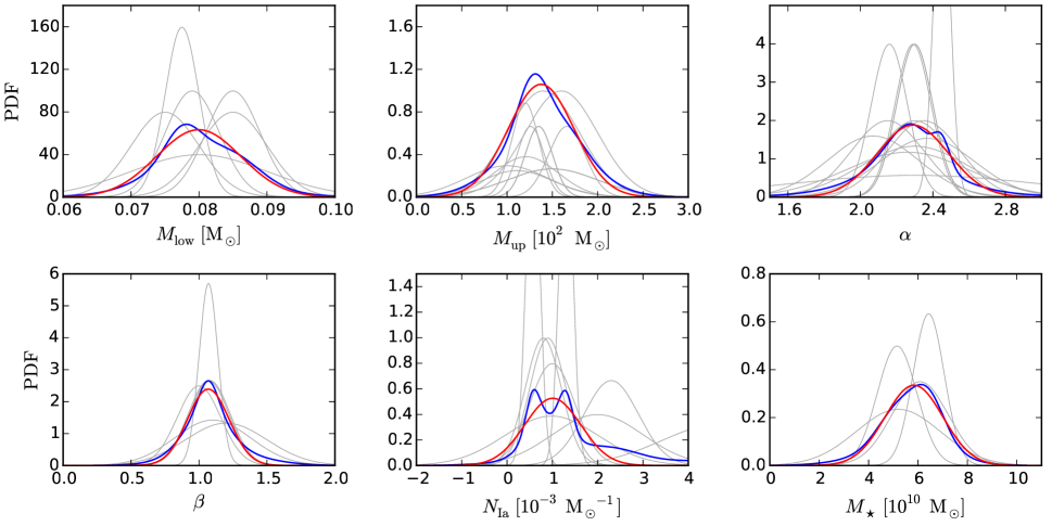
Figure 2.— Probability distribution functions of six of our seven input parameters. The gray, blue, and red lines represent respectively the different observational constraints, the normalized sum of these constraints, and the Gaussian fit of the normalized sum. In the $M_{\mathrm{up}}$ panel, most of the gray lines are actually not normalized to one. Since the mass of the most massive star varies from one stellar cluster to another, we wanted each cluster considered in Table LABEL:tab_uncer_m_up to have the same statistical weight. To do so, the normalization factor of each study has been divided by the number of studies that focused on the same cluster.

Because the most massive stars available in our set of yields is $25\,$M${}_{\odot}\,$(except for zero-metallicity stars), and because of the observed black hole mass distribution, we introduce an initial stellar mass threshold $M_{\mathrm{thresh}}$ of $30\,$M_⊙ above which stars do not release any ejecta. We added this parameter by simplicity, since we are not sure yet how to treat the most massive stars within a SSP. It is beyond the scope of this paper to study how this threshold impacts our results. However, because of this choice, the impact of the upper mass limit of the IMF is underestimated in our work (see Section 3.2). It is worth noting that an initial stellar mass threshold may not exist. Recent simulations by Ugliano et al. (2012) suggests that direct black hole formation and successful CC explosion are both possible outcomes for progenitor stars more massive than 15 M_⊙, with no direct correlation with the initial stellar mass. A further source of complications is given by the lack of observations of CC SN progenitors with initial mass above $\sim$ $18\,$M_⊙ (Smartt 2015), which is far below what is usually assumed in chemical evolution models.

3.9.2 Transition Metallicity

All of our simulations start with a gas reservoir that has a primordial composition. We first use the zero-metallicity yields of Heger & Woosley (2010) until the gas reservoir becomes enriched with metals. When that happens, we switch and instead use the yields for $Z=10^{-4}$ (currently the lowest metallicity available with NuGrid), until the metallicity of the gas actually reaches $Z=10^{-4}$ ([Fe/H] $\simeq$ $-2.3$), above which we start to interpolate the yields according to the metallicity. We therefore never interpolate the yields when the gas reservoir has a non-zero metallicity between $Z=0$ and $Z=10^{-4}$, since we use the logarithm of $Z$ for our interpolations. There is, instead, a transition metallicity $Z_{\mathrm{trans}}$ above which we stop using the zero-metallicity yields. It is worth noting that several studies do support the existence of a transition metallicity around 10${}^{-5}-10^{-3}$ $Z_{\odot}$, between metal-free and metal-poor stars (Bromm et al. 2001; Bromm & Loeb 2003; Schneider et al. 2006; Clark et al. 2008; Dopcke et al. 2011; Schneider et al. 2012; Meece et al. 2014; Smith et al. 2015). However, in our case, we do not fix the value of $Z_{\mathrm{trans}}$. It simply refers to the first non-zero metallicity occurring in the simulations, which can differ from one run to another depending on the values of our input parameters.

3.9.3 Minimum Mass for CC SNe

In the calculation of the stellar ejecta coming out of SSPs, we assume a transition initial stellar mass $M_{\mathrm{trans}}$, fixed a $8\,$M_⊙, above which stars produce CC SNe. According to several studies, this delimitation between intermediate-mass and massive stars should roughly be between 7 and $10\,$M_⊙ (e.g., Timmes et al. 1996; Poelarends et al. 2008; Smartt 2009; Jones et al. 2013; Farmer et al. 2015; Woosley & Heger 2015). The value of this parameter is mainly affected by the physics assumptions made in stellar models. Since our work in this paper focusses on the impact of uncertainties in the measurements of input parameters, and not on the impact of stellar modeling assumptions, $M_{\mathrm{trans}}$ is kept constant at $8\,$M_⊙ in all of our simulations, although recent simulations of super-AGB stars suggest a higher value (see Poelarends et al. 2008; Jones et al. 2013; Farmer et al. 2015). We do, however, consider the lower mass limit of the IMF in the uncertainty calculation even if its value and uncertainty depends on modeling assumptions in stellar models. We only do this because we want to have a complete sampling of the parameters describing the IMF.

3.9.4 SNe Ia Progenitors

In the calculation of the rate of SNe Ia and its normalization, we need to define the explosion progenitors in order to calculate the fraction of white dwarfs used in equations (4) and (5). According to many studies, those progenitors should be stars with initial masses between 3 and $8\,$M_⊙ (e.g., Dahlen et al. 2004; Maoz & Mannucci 2012). However, there is no uncertainty derived for the lower and upper limits of this mass interval. Using 3 and $8\,$M_⊙ is therefore an assumption rather than a measurement with an uncertainty. We do not consider the different evolutionary channels and the possibility that different types of SN Ia may contribute to the chemical inventory of galaxies with relatively different delay times and different numbers (e.g., Hillebrandt et al. 2013; Seitenzahl et al. 2013; Kobayashi et al. 2015; Marquardt et al. 2015). Therefore, the SN Ia contribution must be considered in our work to be an average representative of different potential SN Ia populations.

4. Probability Distribution Functions

In order to consider all the studies compiled in the previous section, we first associated a Gaussian function to each one of them, by centering the function on the mean value, taking the uncertainty as the standard deviation $\sigma$, and finally normalizing to one (gray lines in Figure 2). Our goal here is not to investigate which works are the most relevant, but rather to use all of them to establish an order of magnitude of the current state of uncertainties regarding these observations. For each parameter, we therefore summed all the Gaussians, normalized the resulting curve to one (blue lines), and fitted a new Gaussian function on top of this resulting curve (red lines).

Table 7List of the seven input parameters used in this work to generate uncertainties in our numerical predictions. The value and uncertainty of each parameter are the mean value and the standard deviation taken from the corresponding Gaussian fit presented in Figure 2.

Parameter	Description	Typical value	References
Simple Stellar Population
$M_{\rm low}$	Lower mass limit of the IMF [$10^{-2}\,$M⊙]	8.00 $\pm$ 0.62	Table LABEL:tab_uncer_m_low
$M_{\rm up}$	Upper mass limit of the IMF [M⊙]	138 $\pm$ 36	Table LABEL:tab_uncer_m_up
$\alpha$	Slope of the IMF	2.29 $\pm$ 0.20	Table LABEL:tab_uncer_imf
$\beta$	Slope of the DTD of SNe Ia	1.07 $\pm$ 0.15	Table LABEL:tab_uncer_dtd
$N_{\rm Ia}$	Number of SNe Ia [$10^{-3}$ M${}_{\odot}^{-1}$]	1.01 $\pm$ 0.62	Table LABEL:tab_uncer_NIa
Galaxy
$M_{\star}$	Current stellar mass∗ [$10^{10}\,$M⊙]	5.84 $\pm$ 1.17	Table LABEL:tab_uncer_M_stel
$M_{\mathrm{gas},f}$	Current mass of gas∗∗ [$10^{9}\,$M⊙]	9.2 $\pm$ 5.3	Kubryk et al. (2015)
∗   This parameter is used to calibrate the SFH (see Section 3.6).
∗∗This parameter is used to derive the initial mass of gas (see equation 8).

We used the mean and the standard deviation of the fitted functions to set the typical value and the uncertainty of our model input parameters (Table LABEL:tab_param). However, it should be kept in mind that these numbers are the result of assuming that all the works presented in this section are both independent and equally significant. Neither of these assumptions is true, strictly speaking; multiple different observational estimates use the same astronomical objects to derive constraints, and the techniques used are of varying quality and sophistication, and have different attendant systematic errors. That said, the degree of accuracy of the assumptions of independence and equal significance is both hard to quantify and to express statistically, and thus we use the fitting technique described above to give an approximate description of the uncertainty in our knowledge.

To incorporate these input uncertainties into galactic chemical evolution predictions, we use a Monte Carlo algorithm and run several simulations where the value of each parameter are assumed to be independent, and are randomly selected using its fitted Gaussian function as a PDF. When using this approach, for a parameter having a PDF given by $g(x)$, the probability of randomly selecting a certain value $x_{r}$ is directly proportional to $g(x_{r})$. In other words, values close to the mean value $x_{0}$ are more likely to be picked than values that are further away, simply because the Gaussian PDF $g(x)$ reaches its global maxima when $x=x_{0}$. As shown in Figure 2, some PDFs can generate negative values for our parameters, which is not physical. In the code, we limit our random selection to positive values only.

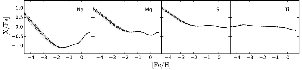
Figure 3.— Predicted chemical abundances relative to Fe and their uncertainties, generated by varying only the current stellar mass ($M_{\star,f}$) and the current mass of gas ($M_{\mathrm{gas},f}$), as a function of [Fe/H] for four elements. The solid lines represent the median values whereas the dashed and dotted lines are the 68% and 95% confidence levels.

This method enables the exploration of a wide range of model input parameters, and also takes into consideration the notion that some values of these parameters are more probable than others. By running a significant number of simulations using this technique, one ends up having many predicted model outputs that cover a range of possible solutions, but where most of the predictions are located near the most probable solution. In other words, the PDF of an input parameter, as processed by the model, induces a related distribution function of predictions related to the evolution of each element as a function of [Fe/H]. Given the complexity of even a simple chemical evolution model, the distribution functions of the input parameters and the model outputs are not necessarily functionally related – as shown in the next sections, even if Gaussian functions are assumed for the PDF of each input parameter, the induced PDFs of the observational predictions are not necessarily Gaussian.

5. Results

The goal of this paper is to illustrate and quantify the impact of input parameters on the level of uncertainty associated with one-zone galactic chemical evolution calculations. To do so, we first ran 700 simulations where all the input parameters were independently and simultaneously selected using the Gaussian probability distribution functions described in Section 4. Then, we took each parameter individually and ran an additional set of 300 simulations where we only varied the considered parameter and kept all the others at their most probable value. This enabled us to have an idea of the contribution of each parameter on the overall uncertainty. We also ran another set of 300 simulations where we simultaneously varied $M_{\star,f}$ and $M_{\mathrm{gas},f}$ (see Section 5.1), since they both affect our numerical predictions in a similar way.

Throughout this section, we do not show any figure regarding the lower and upper mass limits of the IMF, because our simulations demonstrated that these two parameter do not generate a significant amount of uncertainty. This is mainly because the stellar yields in this work are only applied on stars with initial mass between 1 and $30\,$M_⊙ (see Sections 3.2 and 3.9.1 for discussions).

5.1. Speed of the Early Chemical Enrichment

Although the current analysis is very specific to our choice of galactic setup, this section gives the logic behind the generation of uncertainty caused by the parameters regulating the final mass of gas and the stellar mass formed during a simulation. Figure 3 presents chemical evolution predictions for four elements where only $M_{\star,f}$ and $M_{\mathrm{gas},f}$ have been varied. For each plotted element, the gray shaded area illustrates at a given metallicity the full range of possible solutions, whereas the solid, dashed, and dotted lines represent the median value and the 68% and 95% confidence levels, respectively. As shown in this figure, there is a clear correlation between the level of uncertainty and the steepness of the slope of [X/Fe] for [Fe/H] $\lesssim$ $-2$.

Figure 4.— Predicted chemical abundances relative to Fe and their uncertainties, generated by varying only the number of SNe Ia ($N_{\mathrm{Ia}}$), as a function of [Fe/H] for 16 elements. The lines are the same as in Figure 3.

Modifying the final mass of gas and the final stellar mass varies the initial stellar-to-gas mass ratio at the beginning of our simulations. The early [Fe/H] concentration is therefore affected by these parameters because the stellar mass sets the amount of iron ejected by stars and the mass of gas sets the amount of hydrogen in the gas reservoir. However, having a larger or smaller stellar concentration does not modify the [X/Fe] abundances, since those are determined by the ejecta of the first stellar populations. The uncertainties seen in Figure 3 are then mainly generated by horizontal shifts toward higher or lower [Fe/H], which have a greater impact when the element under consideration has a steep slope in its [X/Fe] evolution. However, overall, the uncertainties generated by $M_{\star,f}$ and $M_{\mathrm{gas},f}$ are not significant in our case.

5.2. SNe Ia and Late Enrichment

Figure 4 presents the uncertainty caused by $N_{\mathrm{Ia}}$, the total number of Type Ia explosions that occur per unit of solar mass formed in an SSP. The first noticeable feature is the lack of uncertainty below [Fe/H] $\sim$ $-1.5$, which is caused by the delay between the formation of intermediate-mass stars and the onset of the first SNe Ia. In our case, this [Fe/H] value is associated with a galactic age of $\sim\,150$ Myr. For the Milky Way, observations suggest that SNe Ia only started to be relevant around [Fe/H] $\sim$ $1$ (e.g., Matteucci & Greggio 1986; Chiappini et al. 2001). This discrepancy is mainly caused by our closed-box assumption. Indeed, by having the entire gas reservoir at the beginning of simulations, instead of gradually adding gas with inflows, there is an undesirable high initial gas-to-stellar mass ratio that dilutes the metals ejected by the first stellar populations (see also Lynden-Bell 1975; Chiosi 1980). This reduces the rate at which [Fe/H] is increasing and moves the onset of SNe Ia to metallicities lower than what is expected from observations.

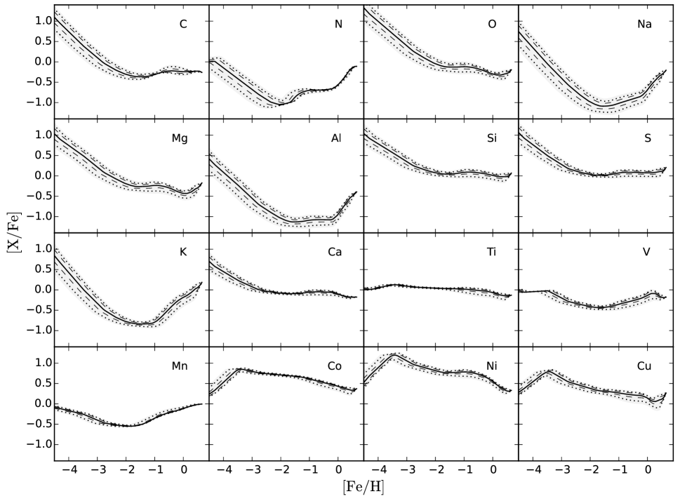
Figure 5.— Predicted chemical abundances relative to Fe and their uncertainties, generated by varying only the slope of the high-mass end of the stellar IMF ($\alpha$), as a function of [Fe/H] for 16 elements. The lines are the same as in Figure 3.

For the vast majority of elements presented in Figure 4, modifying the number of SNe Ia generates a diagonal shift in the predictions (along the upper left to lower right diagonal). For example, adding more Type Ia explosions will increase [Fe/H] but will also decrease [X/Fe]. This is why there is generally a diagonal cut in the uncertainty shape at high [Fe/H]. For metallicities that are below the beginning of this diagonal cut, all the 300 possible predictions are included in the statistical analysis. But at higher metallicities, only a fraction of these predictions have sufficient SNe Ia to reach such high iron abundances.

As seen in Figure 4, the level of uncertainty is not always the same from one element to another. Elements that are not significantly produced by SNe Ia, such as the CNO elements, are the most affected by the $N_{\mathrm{Ia}}$ parameter. This is because the variation of the number of explosions only modifies the iron content in the [X/Fe] vs [Fe/H] relations. But in the case of other elements, such as Ca and Ni, for which SNe Ia have a contribution of about 10% to 50% (according to our set of yields), the predictions become less affected by the number of explosions. The idea behind this trend is that increasing $N_{\mathrm{Ia}}$ forces the gas reservoir to look like the ejecta of an SN Ia. Since these explosions already contribute significantly to the production of such elements, the chemical abundances relative to iron eventually become saturated when $N_{\mathrm{Ia}}$ is increased.

Because of the direction of the diagonal shift in the [X/Fe] vs [Fe/H] space caused by the variation of $N_{\mathrm{Ia}}$, elements showing a positive slope in their evolution (increasing [X/Fe] with increasing [Fe/H]) will systematically tend to have a higher level of uncertainty than the ones showing a negative slope (decreasing [X/Fe] with increasing [Fe/H]). Mn is an exception, since this element and Fe are both mainly ejected by SNe Ia. As seen in Tolstoy et al. (2009), the evolution of alpha elements relative to iron in nearby dwarf spheroidals usually shows a steeper negative slope than in the Milky Way. This means that the variation of $N_{\mathrm{Ia}}$ should generate less uncertainty when tuning a galactic chemical evolution model to represent a dwarf galaxy, even if SNe Ia contribute significantly to their chemical evolution (e.g., Venn et al. 2012). As was pointed out in the previous section, the level of uncertainty is tightly connected to the specific shape and slope of each prediction, which in turn is directly related to the choice of stellar yields and the type of galaxy considered.

Figure 6.— Predicted chemical abundances relative to Fe and their uncertainties as a function of [Fe/H] for 16 elements, including all model parameters varied simultaneously. The lines are the same as in Figure 3.

The slope of the DTD function of SNe Ia, $\beta$, has an impact similar to that of the total number of explosions in the sense that it also produces diagonal shifts in the predictions. However, the slope of the DTD function does not modify the total number of explosions associated with each stellar population. The uncertainties generated by $\beta$ are on average three times lower than the ones generated by $N_{\mathrm{Ia}}$, which is mainly caused by the different input level of uncertainty of these two parameters (see Table LABEL:tab_param).

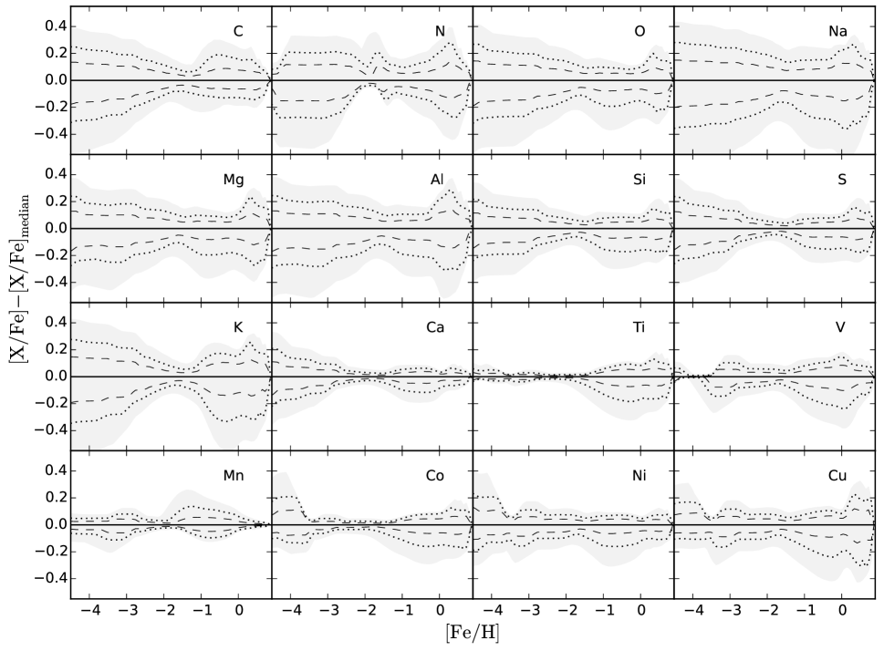
Figure 7.— Uncertainties in our predictions as a function of [Fe/H] for 16 elements, including all model parameters varied simultaneously. This is the analogous of Figure 6 where the median values have been subtracted from all predictions.

5.3. Slope of the IMF and Stellar Yields

The slope of the high-mass end of the IMF is the most significant parameter in the generation of uncertainties in our model. As seen in Figure 5, this parameter impacts the predictions at every metallicity. Although the uncertainties vary substantially from one element to another, the most important notion to remember is that the IMF mostly affects the prediction when iron and the considered elements are produced in different stars. Otherwise, modifying the relative numbers of stars with different initial mass will not change the [X/Fe] abundance ratios, although it can modify [Fe/H].

It is instructive to consider the very-low-metallicity parts of Figure 5 below [Fe/H] $\sim$ $-2$. At these metallicities, no SN Ia has occurred yet and the chemical evolution is then purely driven by the yields of massive stars at Z $=$ 0 and 10^-4 (see Section 3.9.2), which simplifies the analysis. As an example, in the case of C, N, O, Na, Mg, and Al, the level of uncertainty has a continuous-looking shape, since these elements and Fe are not ejected by the same stars, both at Z $=$ 0 and 10^-4. For Si, S, K, and Ca, there is a tightening feature around [Fe/H] of $-2$ since these elements and Fe are mainly ejected by the same stars at Z $=$ 10^-4, but by different stars at Z $=$ 0. Only the very-low-metallicity end of [X/Fe] is then affected by the IMF. For Ti and Mn, their evolution do not significantly depend on the slope of the IMF since they are all generally ejected by the same stars that the ones responsible for the ejection of Fe, for Z $=$ 0 and 10^-4. This demonstrates that the uncertainties produced by the slope of the IMF are directly connected to the choice of stellar yields and the number of metallicities available with these yields. The same logic is applicable at higher metallicities. The analysis is, however, somewhat more complex since iron now comes from both the CC SNe of young stellar populations and the SNe Ia of older stellar populations.

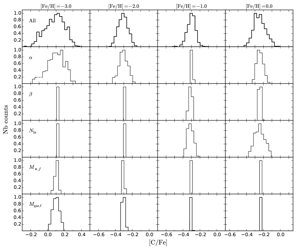
Figure 8.— Probability distribution functions of [C$/$Fe] taken at different [Fe$/$H]. In the first row, all the parameters are included in the uncertainties. In the remaining rows, each parameter has been considered individually in order to provide an estimate of their contribution to the overall uncertainty.

Carbon shows an interesting low level of uncertainties around [Fe/H] of $-$1 (see Figure 5). This special case corresponds to a cross-over point, which means that a prediction below the median at [Fe/H] $<$ $-$1 will be above the median at [Fe/H] $>$ $-$1, and vice versa. From our set of stellar yields, carbon is mainly ejected by low-mass stars, which explains the [C/Fe] bump seen at [Fe/H] $\sim$ $-0.5$. In addition, carbon yields at $Z=10^{-4}$ are 50% larger compared to yields at $Z=0.001$, and 85% larger compared to yields at $Z=0.006$. Having a steeper IMF creates more low-metallicity stars, since [Fe/H] initially increases at a slower pace due to the reduced number of massive stars. This case corresponds to the lines far below the median line of [C/Fe] at early times. However, once low-mass stars start to contribute to the ejection of carbon, the high number of low-metallicity stars maximizes the amplitude of the bump located at [Fe/H] $\sim$ $-0.5$, thus creating the cross-over point.

5.4. Overall Uncertainty

Figures 6 and 7 show the overall uncertainty associated with our predictions coming from our one-zone model, which is the result of varying all the parameters simultaneously. The overall level of uncertainty evolves as a function of [Fe/H] and varies from one element to another. By combining these figures with the results presented in the previous sections, it is now possible to analyze the uncertainty of each element in a different manner. As an example, the top row of Figure 8 presents the overall PDFs of [C/Fe] for four different [Fe/H] values, whereas the following rows illustrate the contribution of the individual parameters. This figure is useful for visualizing which input parameters have the most impact and at which metallicity. In the case of carbon, the slope of the IMF is the main contributor of the overall uncertainties at low [Fe/H] (i.e., early in the galaxy’s star formation process). At high [Fe/H] (i.e., later in time), the total number of SNe Ia dominates the uncertainties.

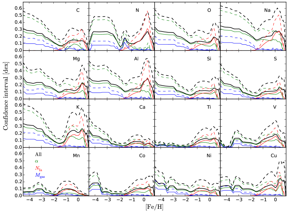
Figure 9.— Evolution of the confidence intervals of [X/Fe] as a function of [Fe/H] and parameters. The solid and dashed lines represent respectively the thickness of the confidence intervals within 68% and 95%. The black lines include all seven parameters in the generation of the uncertainties. The coloured lines, as indicated, show the estimated individual contribution of the three most important parameters.

It is worth noting that summing all of the uncertainties obtained by varying the individual parameters one at a time will not reproduce the overall uncertainty presented in Figures 6 and 7. Indeed, when varying only one parameter, its uncertainty is only induced into a specific prediction, since all of the other parameters are kept constant. However, when all parameters are varied at the same time, the uncertainty induced by a single parameter becomes spread in all the possible predictions generated by the random selection of the other parameters. It is then important to reiterate that our analysis of individual contributions is only an estimate. Nevertheless, it turns out to be an efficient way to evaluate which parameter generates the most uncertainties in galactic chemical evolution models.

In Figure 9, we show a different representation of the information contained in Figure 8, but for all 16 elements discussed in prior sections. We calculate the thickness of the 68% and 95% confidence intervals for every element as a function of [Fe/H]. This figure only includes the overall uncertainties and the contributions of the three parameters that contribute the most to the global uncertainty, which are the slope of the stellar IMF, the total number of SNe Ia, and the final mass of the gas reservoir of the galaxy. A local minimum in the overall uncertainty is often seen around [Fe/H] $\sim$ $-1.5$, which is partially caused by the rise of SNe Ia. For some elements such as Ti, the contribution of the IMF also starts to increase at the same metallicity. As mentioned throughout this paper, the derived amount of uncertainty also depends on the stellar yields and should be taken with caution.

5.5. Impact of the Reference Element

Although the measurement of Fe has observational conveniences, other elements can be used to study the chemical evolution of galaxies (see the discussion found in Cayrel et al. 2004). As an example, the upper panel of Figure 10 presents the overall uncertainty of [Ti/Mg] as a function of [Mg/H]. Compared to Figure 6, the uncertainties in the predictions of Ti at high metallicity are greatly reduced when plotted relative to Mg instead of Fe. This is partially because SNe Ia are not the main source of production of Mg and Ti, which eliminates large amount of uncertainty generated by $N_{\mathrm{Ia}}$, the number of SNe Ia in SSPs (see Section 5.2). On the other hand, because of the uncertainty in the slope of the IMF, the predictions are a lot more uncertain at low metallicity when using Mg instead of Fe, since Ti and the reference element (Mg) are no longer ejected by the same stars in our stellar yields at $Z=0$ and $Z=10^{-4}$.

As seen in the lower panel of Figure 10, the predicted evolution of Mn is now very uncertain when plotted relative to Mg, despite the fact that Mn was one of the elements with the lowest level of uncertainty when plotted relative to Fe (see Figure 6). The element of reference then have a significant impact on the amount of uncertainties generated by input parameters. As a general remark, the predicted evolution of [X/X_ref] as a function of [X_ref/H] will always be more uncertain when the elements X and X_ref are not ejected by the same stars.

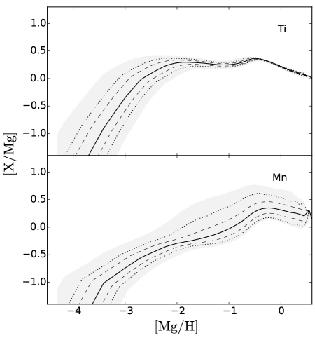
Figure 10.— Predicted chemical abundances and their uncertainties as a function of [Mg/H] for Ti and Mn, including all model parameters varied simultaneously. The lines are the same as in Figure 3.

5.6. Evolution of Individual Elements

Looking at the abundances of one element against another one ([X/X_ref] vs [Y/X_ref]) is convenient for comparing with observational data. However, it is hiding the uncertainties in the evolution of individual elements. As shown in Figure 11, the amount of uncertainty is larger for [X/H] as a function of time than for [X/Fe] as a function of [Fe/H] (see Figure 7). This means the overall amount of uncertainty associated with one specific element depends on the way numerical predictions are shown. For example, Figure 7 suggests that our predictions for Ti are almost free of uncertainty at low metallicity, which is a misleading conclusion when referring to Figures 10 and 11. In this last figure, there is a certain similarity in the shape of the uncertainty envelope (gray shaded area) for Na, Al, and K. As seen in Figure 6, these three elements show a similar U-shape in the [X/Fe]-[Fe/H] space, reinforcing the idea that the level of uncertainty also depends on the global shape of numerical predictions.

6. Discussion

So far, we have demonstrated that some input parameters in a closed-box, single-zone model can induce significant amount of uncertainties in numerical predictions. This is an important step in our long-term project which aims to better quantify the uncertainties inherent in more complex chemical evolution models. Our study is, however, subject to a variety of limitations and caveats. In the next sections, we briefly discuss some of them and highlight additional sources of uncertainty in chemical evolution studies.

6.1. Stellar Yields

For the sake of simplicity, we choose to use a single set of yields, which includes five metallicities between $Z=10^{-4}$ and $Z=0.02$ for massive and AGB stars (see Section 2.2), the SN Ia yields of Thielemann et al. (1986), and the zero-metallicity yields of Heger & Woosley (2010) for the first stellar populations formed in our simulation. It is known that different stellar evolution codes and different research groups produce different nucleosynthetic yields (Gibson 1997, 2002; Romano et al. 2010; Mollá et al. 2015). But, besides the SN Ia and zero-metallicity yields, all of our stellar models have been calculated with the MESA code and were post-processed with NuGrid’s nucleosynthesis code MPPNP in order to have a consistent set of assumptions.

However, even if a set of yields is calculated with the same code, there are always sources of uncertainties attached to nuclear reaction networks and modeling assumptions. For example, the choice of mass cut which defines where the explosion is launched inside a massive star has a significant impact on chemical evolution predictions. In this work, we used a prescription derived by Fryer et al. (2012) (see also Pignatari et al. 2013a) to tune the mass cut of our stellar models in order to reproduce the observed neutron-star and black hole mass distribution functions (Belczynski et al. 2012). The explosive yields generated by this prescription are different than those generated with a mass-cut prescription based on the electronic mass fraction value ($Y_{e}$). This is particularly true for Ni and Cu, as shown in Figure 12. For the explosive yields produced with the $Y_{e}$ prescription, we launched the explosion from the location where $Y_{e}=0.4992$ (see Arnett 1996 for more information). It is however beyond the scope of this paper to fall into a detailed analysis of the impact modeling assumptions in CC SN calculations. A description of the yields produced by different mass-cut prescriptions will be presented in C. Ritter et al. (in preparation).

6.2. Interpolation of Stellar Yields

Because of the large metallicity range covered in galactic chemical evolution, yields are usually interpolated according the logarithm of $Z$. Although we can interpolate between $Z=10^{-4}$ and $Z=0.02$, we cannot follow the same interpolation law between $Z=0$ and $Z=10^{-4}$. Thus, there is no interpolation below [Fe/H] $\simeq-2.3$. The only $Z$-dependency considered in the early chemical evolution is the transition between the use of zero-metallicity yields and $Z=10^{-4}$ yields, which occurs as soon as the primordial gas reservoir becomes enriched by the first stars. The lack of very-low-metallicity stellar yields, especially for CC SNe, represents an additional hidden source of uncertainty for numerical predictions at [Fe/H] $\lesssim$ $-2.5$. This situation also occurs with the yields of Woosley & Weaver (1995) and Nomoto et al. (2006). But it should be noted that efforts has been made to provide stellar yields at very-low metallcity (e.g., Chieffi & Limongi 2004; Hirschi 2007). However, the calculation of very-low-metallicity yields is challenging and involves physical problems, such as hydrogen ingestion events, that are difficult to solve in one-dimensional calculations (e.g., Herwig et al. 2011).

Even when interpolation is possible between metallicities, the number of metallicity bins in our input yields, and also the number of stellar mass bins, may substantially affect our results. The extent of this is unclear – no study has been made to determine the “minimum acceptable” grid of models.

6.3. Galactic Chemical Evolution Model

We use a closed-box model with a constant star formation efficiency. We explicitly ignore inflow of low-metallicity gas (i.e., accretion), outflow of high-metallicity gas (i.e., galactic winds), and all aspects of galaxy formation including the growth of the galactic potential well, and stochasticity due to mergers. This was done deliberately – we want to consider the simplest possible model. Considering more complex models surely add more realism and flexibility in the predictions, but it also introduce new sources of uncertainty as more parameters and more assumptions are implemented. In future work, we plan to highlight this by expanding our uncertainty study beyond the closed-box model.

6.4. Initial Mass Function

Although we used a Chabrier IMF, there are other possible IMFs (Kroupa, Salpeter, lognormal, etc.) that have been used to fit the local observational data. We cannot readily include them simultaneously with the approach described in Section 4, because these IMFs have different functional forms and often possess discontinuities. We can perform our analysis for other IMFs, but the results are likely to remain qualitatively the same, though quantitatively somewhat different. We further assume that the stellar IMF is the same in all young star clusters, and implicitly everywhere in the universe at all times. For example, we assume extremely low-metallicity stars have the same IMF as solar-metallicity stars. This is not particularly defensible – environment and redshift possibly have an effect on stellar IMF (e.g., Tumlinson 2007; Cappellari et al. 2012; Conroy & van Dokkum 2012; Chattopadhyay et al. 2015). The PDF of our input parameters defining the IMF could in fact vary as a function of time in our simulations, which would modify the contribution of $\alpha$, $M_{\mathrm{low}}$, and $M_{\mathrm{up}}$ on the generation of uncertainties.

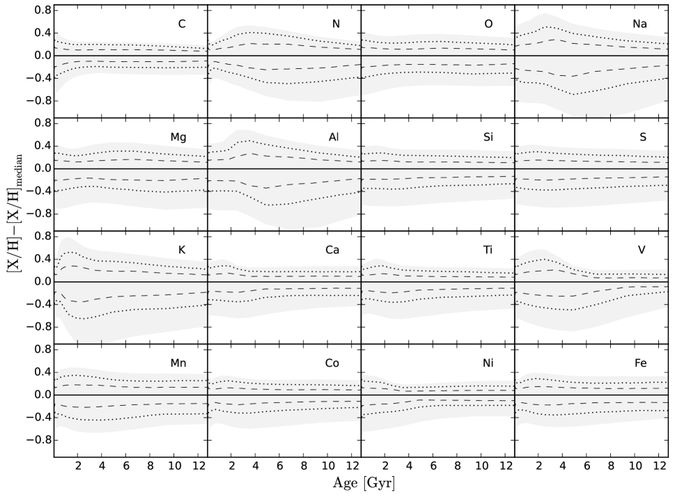
Figure 11.— Uncertainties in our predictions as a function of galactic age for 16 elements relative to H, including all model parameters varied simultaneously. The lines are the same as in Figure 3.

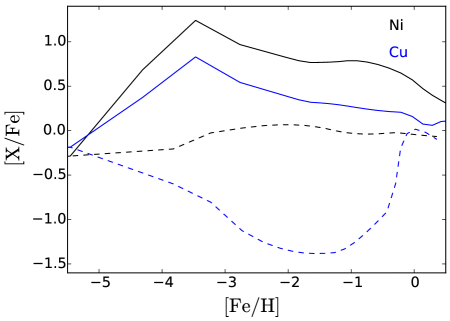
Figure 12.— Predicted abundances of Ni and Cu, relative to Fe, as a function of [Fe/H] using two different mass-cut prescriptions for the CC SN yield calculations. The solid lines represent the prescription of Fryer et al. (2012), designed to reproduce the observed neutron-star and black-hole mass distribution functions, while the dashed lines represent the Ye prescription (see text in Section 6.1). For this figure, we set all parameters to their typical value (see Table LABEL:tab_param).

We only include the contribution of CC SNe for stars with initial mass below $M_{\mathrm{thresh}}=30\,$M_⊙. If we were to include them, deriving the yields of those more massive stars becomes tricky and uncertain, since we need to rely on an extrapolation rather than on a safer interpolation between stellar models. The result of such an extrapolation depends on the available maximum stellar initial mass included in the set of yields, which is $25\,$M_⊙ in our case (except for the zero-metallicity yields of Heger & Woosley 2010). Because of this, and because $M_{\mathrm{thresh}}$ is not yet an observationally estimated quantity, addressing this issue in more detail is beyond the scope of this paper. Moreover, there are still uncertainties regarding the fate of stars more massive than $\sim$ $15\,$M_⊙ (see Section 3.9.1).

6.5. Generation of Uncertainties

The method that we use to calculate the Gaussian distributions describing our input parameters is relatively simple – we create a distribution from the normalized values of the parameters from a variety of observations and fit a Gaussian distribution to it, which gives us a mean and a standard deviation. This assumes that the observations are independent and use the same methods, which is not true. In reality, most observational works use different approaches varying in accuracy and sophistication. It is difficult and typically highly subjective to quantify the statistical weight of each observed quantity, which would nevertheless be useful in order to generate more representative PDFs.

We assume that all of our input parameters are uncorrelated. This allows us to randomly and independently choose their value in each simulation. However, there must be correlations, especially between the slope of the IMF and the number of SNe Ia. Adding a correlation between these two parameters would increase the amount of uncertainty at the high-metallicity end of our [X/Fe]-[Fe/H] predictions. All the 16 considered elements, besides C, N, and Mn, are mainly ejected by massive stars. A correlation between the IMF and the number of SNe Ia would therefore favors more SNe Ia (more iron) when the number of massive stars is reduced, and vice-versa. For C and N, such a correlation would reduce the level of uncertainty, as these elements are mainly ejected by low- and intermediate-mass stars, which includes the progenitors of SNe Ia.

Some parameters have not been included in the generation of the uncertainties (see Section 3.9). In addition, we did not considered uncertainties associated with stellar yields, modeling assumptions, star formation histories, and galaxy evolution environment. The uncertainties derived in this paper thus represent a lower limit of the real uncertainties inherent in chemical evolution models.

7. Summary and Conclusions

Using a simple chemical evolution code, the goal of this paper was to quantify the uncertainties induced in numerical predictions by seven input parameters describing the IMF, the rate of SNe Ia, and the basic properties of the Milky Way. To do so, we compiled observational and numerical work from the literature in order to derive the typical value and the PDF of each parameter. We then ran several hundred simulations using a Monte Carlo algorithm to randomly select the input parameters from their individually determined PDFs. Using this approach, we have been able to quantify in a statistical manner the uncertainties in the chemical evolution of our simulated galaxies by providing the most probable predictions along with their 68% and 95% confidence levels. Our main conclusions are the following.

• When considering the variation of all parameters simultaneously, these parameters produce an overall uncertainty roughly between 0 and 0.6 dex when abundances are plotted against metallicity. However, the level of uncertainty is metallicity-dependent and is different from one element to another, since every element has its own evolution pattern and production site. The amount of uncertainty can reach 1 dex when looking at the evolution of an individual element as a function of time instead of metallicity.

• The overall uncertainties are produced by a combination of different input parameters that contribute at different metallicities. The current mass of gas and the current stellar mass of the galaxy only affect the early chemical evolution below [Fe/H] $\sim$ $-2$. On the other hand, the slope of the delay-time distribution function and the total number of SNe Ia only affect the predictions above [Fe/H] $\sim$ $-1.5$, whereas the slope of the IMF has generally an impact at all metallicities.

• Among the seven input parameters included in this study, the slope of the high-mass end of the stellar IMF and the total number of SNe Ia contribute the most to the overall uncertainties when abundances are plotted against metallicity. These parameters have a stronger impact when the considered element and the reference element (e.g., iron) are not ejected by the same stars.

• Input parameters do not modify the overall trends seen in numerical predictions. Characteristic features in the [X/Fe]$-$[Fe/H] or [X/Mg]$-$[Mg/H] space, such as the slope and the curvature of the predictions, or the presence of bumps, cannot be modified by varying the input parameters. Such features are mainly caused by the choice of stellar yields and the type of galaxy considered. In other words, the input parameters only spread their uncertainties on top of predictions already pre-defined by these two last ingredients.

Our work showed that some input parameters in one-zone, closed-box calculations add a significant amount of uncertainty that is often comparable to or even larger than the scatter seen in observational data, despite the fact that we did not include the uncertainties associated with stellar yields, galaxy formation, and modeling assumptions. It is then very clear that the uncertainties derived in this paper represent only a lower limit of what must be the real and concerning amount of uncertainty inherent in galactic chemical evolution models. For the moment, we cannot apply our uncertainty quantification to more realistic models such as multi-zone and open-box models or chemo-dynamical simulations, since further investigation is needed. However, all of those more sophisticated models should also be affected by their own parameters in a similar way. Most of the parameters explored in this work, especially for the IMF and SNe Ia, are fundamental and must somehow be implemented in every chemical evolution model or simulation.

References

- Arnett (1996) Arnett, D. 1996, Supernovae and Nucleosynthesis: An Investigation of the History of Matter from the Big Bang to the Present (Princeton University Press)
- Arnett et al. (2010) Arnett, D., Meakin, C., & Young, P. A. 2010, ApJ, 710, 1619