1 Introduction
An interesting area of electromagnetism for its applications and the arising theoretical problems is the scattering process from obliquely incident time-harmonic plane waves by an infinitely long cylinder. The basic waves in the propagation domain satisfy Maxwell’s equations [1 , 3 , 16 , 18 ] and due to the symmetry of the problem it is equivalent to find two scalar fields satisfying a pair of two-dimensional Helmholtz equations with different wavenumbers. The complication appears in the boundary conditions. Even for the case of a perfect conductor, in the boundary conditions appear tangential derivatives which make the analysis more difficult.
There are many studies providing analytical or numerical solutions [2 , 13 , 19 , 20 , 21 , 22 , 24 , 25 ] . The proposed methods are based on specific geometries or well known numerical schemes without examining the well-posedness of the corresponding boundary value problem.
Recently, Wang and Nakamura [23 ] used a more elegant theoretical analysis to prove well-posedness of the problem based on the integral equation approach. They proved theoretical and numerical results for the case of homogeneous impedance cylinder using integral equations. For the theoretical analysis they used properties of the Cauchy singular integrals and proved that the derived system is of Fredholm type with index zero. For the numerical results they applied a specific decomposition of the kernels and formulations using Hilbert’s and Symm’s integral operators. Considering trigonometric interpolation, they introduced an efficient numerical scheme.
The case for general dielectric cylinders is not considered yet, however the same authors, in a later work [17 ] , investigated a more complicated model having also a non-homogeneous part, in the sense that the permittivity and the permeability of the exterior medium are non-constants and smooth in a bounded domain surrounding the cylinder. The main theoretical analysis providing uniqueness and existence in non-homogeneous materials is much harder. For the well-posedness they used the Lax-Phillips method [7 ] .
In this work, we examine the case of infinite dielectric cylinder illuminated by a transverse magnetic polarized electromagnetic plane wave, known as oblique incidence. More precisely, in the second Section starting from Maxwell’s equations we describe initially the derivation of the mathematical model for the scattering process from obliquely incident time-harmonic plane waves for the case of infinite inhomogeneous cylinder. We assume that transmission conditions hold on the boundary. The boundary conditions involve normal and tangential derivatives of the fields.
In Section 3, we formulate the direct problem in differential form. We derive the Helmholtz equations and the exact form of the boundary conditions in the case of homogeneous cylinder. We prove that the problem is uniquely solvable using Green’s formulas and Rellich’s lemma. Considering the direct method, initially applied in transmission problems in [5 , 8 , 9 ] , we formulate the problem into an equivalent system of integral equations. We show that this system is of Fredholm type in an appropriate Sobolev space setting. Due to uniqueness of the boundary value problem existence follows from Fredholm alternative. The system consists of compact, singular and hypersingular operators. We consider Maue’s formula [14 ] , as in the case of the normal derivative of the double layer potential, to reduce the hypersingularity of the tangential derivative of the double layer potential.
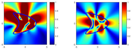
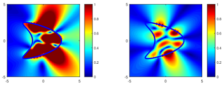
In the last Section we investigate numerically the problem by a collocation method based on Kress’s method for two dimensional integral equation with strongly singular operators [10 ] . We transform the system of integral equations to a linear system by parametrizing the operators and considering well-known quadrature rules. We derive accurate numerical results for the four fields, interior and exterior, and we compute numerically the far-field patterns of the two exterior fields computed for a specific boundary value problem. Namely, we consider boundary data corresponding to analytic fields derived from point sources, where the interior and exterior fields have singularities outside of their domain of consideration.
2 Formulation of the direct scattering problem for an inhomogeneous cylinder
We consider the scattering problem of an electromagnetic wave by a penetrable cylinder in ℝ 3 superscript ℝ 3 \mathbbm{R}^{3} 𝒙 = ( x , y , z ) ∈ ℝ 3 , 𝒙 𝑥 𝑦 𝑧 superscript ℝ 3 \bm{x}=(x,y,z)\in\mathbbm{R}^{3}, Ω i n t = { 𝒙 : ( x , y ) ∈ Ω , z ∈ ℝ } , subscript Ω 𝑖 𝑛 𝑡 conditional-set 𝒙 formulae-sequence 𝑥 𝑦 Ω 𝑧 ℝ \Omega_{int}=\{\bm{x}:(x,y)\in\Omega,z\in\mathbbm{R}\}, Ω Ω \Omega ℝ 2 superscript ℝ 2 \mathbbm{R}^{2} Γ . Γ \Gamma. Ω i n t subscript Ω 𝑖 𝑛 𝑡 \Omega_{int} z 𝑧 z Ω Ω \Omega ϵ 0 subscript italic-ϵ 0 \epsilon_{0} μ 0 subscript 𝜇 0 \mu_{0} Ω e x t := ℝ 3 ∖ Ω ¯ i n t . assign subscript Ω 𝑒 𝑥 𝑡 superscript ℝ 3 subscript ¯ Ω 𝑖 𝑛 𝑡 \Omega_{ext}:=\mathbbm{R}^{3}\setminus\overline{\Omega}_{int}. Ω i n t subscript Ω 𝑖 𝑛 𝑡 \Omega_{int} μ ( 𝒙 ) = μ ( x , y ) 𝜇 𝒙 𝜇 𝑥 𝑦 \mu(\bm{x})=\mu(x,y) ϵ ( 𝒙 ) = ϵ ( x , y ) italic-ϵ 𝒙 italic-ϵ 𝑥 𝑦 \epsilon(\bm{x})=\epsilon(x,y) ( x , y ) ∈ Ω , z ∈ ℝ . formulae-sequence 𝑥 𝑦 Ω 𝑧 ℝ (x,y)\in\Omega,\,z\in\mathbbm{R}.
We define for 𝒙 ∈ Ω e x t , t ∈ ℝ formulae-sequence 𝒙 subscript Ω 𝑒 𝑥 𝑡 𝑡 ℝ \bm{x}\in\Omega_{ext},\,t\in\mathbbm{R} 𝑯 e x t ( 𝒙 , t ) superscript 𝑯 𝑒 𝑥 𝑡 𝒙 𝑡 \bm{H}^{ext}(\bm{x},t) 𝑬 e x t ( 𝒙 , t ) superscript 𝑬 𝑒 𝑥 𝑡 𝒙 𝑡 \bm{E}^{ext}(\bm{x},t) 𝑯 i n t ( 𝒙 , t ) superscript 𝑯 𝑖 𝑛 𝑡 𝒙 𝑡 \bm{H}^{int}(\bm{x},t) 𝑬 i n t ( 𝒙 , t ) superscript 𝑬 𝑖 𝑛 𝑡 𝒙 𝑡 \bm{E}^{int}(\bm{x},t) 𝒙 ∈ Ω i n t , t ∈ ℝ . formulae-sequence 𝒙 subscript Ω 𝑖 𝑛 𝑡 𝑡 ℝ \bm{x}\in\Omega_{int},\,t\in\mathbbm{R}.
∇ × 𝑬 e x t + μ 0 ∂ 𝑯 e x t ∂ t \displaystyle\operatorname{\nabla\times}\bm{E}^{ext}+\mu_{0}\frac{\partial\bm{H}^{ext}}{\partial t} = 0 , absent 0 \displaystyle=0, ∇ × 𝑯 e x t − ϵ 0 ∂ 𝑬 e x t ∂ t \displaystyle\operatorname{\nabla\times}\bm{H}^{ext}-\epsilon_{0}\frac{\partial\bm{E}^{ext}}{\partial t} = 0 , absent 0 \displaystyle=0, 𝒙 ∈ Ω e x t , 𝒙 subscript Ω 𝑒 𝑥 𝑡 \displaystyle\bm{x}\in\Omega_{ext}, (1)
∇ × 𝑬 i n t + μ ∂ 𝑯 i n t ∂ t \displaystyle\operatorname{\nabla\times}\bm{E}^{int}+\mu\frac{\partial\bm{H}^{int}}{\partial t} = 0 , absent 0 \displaystyle=0, ∇ × 𝑯 i n t − ϵ ∂ 𝑬 i n t ∂ t \displaystyle\operatorname{\nabla\times}\bm{H}^{int}-\epsilon\frac{\partial\bm{E}^{int}}{\partial t} = 0 , absent 0 \displaystyle=0, 𝒙 ∈ Ω i n t . 𝒙 subscript Ω 𝑖 𝑛 𝑡 \displaystyle\bm{x}\in\Omega_{int}.
On the boundary Γ , Γ \Gamma,
𝒏 ^ × 𝑬 i n t = 𝒏 ^ × 𝑬 e x t , 𝒏 ^ × 𝑯 i n t = 𝒏 ^ × 𝑯 e x t , 𝒙 ∈ Γ , formulae-sequence bold-^ 𝒏 superscript 𝑬 𝑖 𝑛 𝑡 bold-^ 𝒏 superscript 𝑬 𝑒 𝑥 𝑡 formulae-sequence bold-^ 𝒏 superscript 𝑯 𝑖 𝑛 𝑡 bold-^ 𝒏 superscript 𝑯 𝑒 𝑥 𝑡 𝒙 Γ \bm{\hat{n}}\times\bm{E}^{int}=\bm{\hat{n}}\times\bm{E}^{ext},\quad\bm{\hat{n}}\times\bm{H}^{int}=\bm{\hat{n}}\times\bm{H}^{ext},\quad\bm{x}\in\Gamma,
where 𝒏 ^ bold-^ 𝒏 \bm{\hat{n}} Ω e x t subscript Ω 𝑒 𝑥 𝑡 \Omega_{ext}
In order to take advantage of the symmetry of the specific medium, we probe the cylinder with an incident transverse magnetic (TM) polarized electromagnetic plane wave, the so-called oblique incidence in the literature. An arbitrary time-harmonic incident electromagnetic plane wave has the form:
𝑬 i n c ( 𝒙 , t ; 𝒅 ^ , 𝒑 ^ ) superscript 𝑬 𝑖 𝑛 𝑐 𝒙 𝑡 bold-^ 𝒅 bold-^ 𝒑 \displaystyle\bm{E}^{inc}(\bm{x},t;\bm{\hat{d}},\bm{\hat{p}}) = 1 k 0 2 ϵ 0 ∇ × ∇ × ( 𝒑 ^ e i k 0 𝒙 ⋅ 𝒅 ^ ) e − i ω t , \displaystyle=\frac{1}{k_{0}^{2}\sqrt{\epsilon_{0}}}\operatorname{\nabla\times}\operatorname{\nabla\times}\left(\bm{\hat{p}}\,e^{ik_{0}\bm{x}\cdot\bm{\hat{d}}}\right)e^{-i\omega t},
𝑯 i n c ( 𝒙 , t ; 𝒅 ^ , 𝒑 ^ ) superscript 𝑯 𝑖 𝑛 𝑐 𝒙 𝑡 bold-^ 𝒅 bold-^ 𝒑 \displaystyle\bm{H}^{inc}(\bm{x},t;\bm{\hat{d}},\bm{\hat{p}}) = 1 i k 0 μ 0 ∇ × ( 𝒑 ^ e i k 0 𝒙 ⋅ 𝒅 ^ ) e − i ω t , \displaystyle=\frac{1}{ik_{0}\sqrt{\mu_{0}}}\operatorname{\nabla\times}\left(\bm{\hat{p}}\,e^{ik_{0}\bm{x}\cdot\bm{\hat{d}}}\right)e^{-i\omega t},
where ω > 0 𝜔 0 \omega>0 k 0 = ω μ 0 ϵ 0 subscript 𝑘 0 𝜔 subscript 𝜇 0 subscript italic-ϵ 0 k_{0}=\omega\sqrt{\mu_{0}\epsilon_{0}} 𝒑 ^ bold-^ 𝒑 \bm{\hat{p}} 𝒅 ^ bold-^ 𝒅 \bm{\hat{d}} 𝒅 ^ ⟂ 𝒑 ^ . perpendicular-to bold-^ 𝒅 bold-^ 𝒑 \bm{\hat{d}}\perp\bm{\hat{p}}.
In the following, due to the linearity of the problem we suppress the time-dependence and we consider the fields only as functions of the space variable 𝒙 𝒙 \bm{x} θ 𝜃 \theta z 𝑧 z ϕ italic-ϕ \phi 𝒅 ^ bold-^ 𝒅 \bm{\hat{d}} 𝒅 ^ = ( sin θ cos ϕ , sin θ sin ϕ , − cos θ ) bold-^ 𝒅 𝜃 italic-ϕ 𝜃 italic-ϕ 𝜃 \bm{\hat{d}}=(\sin\theta\cos\phi,\sin\theta\sin\phi,-\cos\theta) 𝒑 ^ = ( cos θ cos ϕ , cos θ sin ϕ , sin θ ) , bold-^ 𝒑 𝜃 italic-ϕ 𝜃 italic-ϕ 𝜃 \bm{\hat{p}}=(\cos\theta\cos\phi,\cos\theta\sin\phi,\sin\theta), θ ∈ ( 0 , π / 2 ) ∪ ( π / 2 , π ) . 𝜃 0 𝜋 2 𝜋 2 𝜋 \theta\in(0,\pi/2)\cup(\pi/2,\pi).
𝑬 i n c ( 𝒙 ; 𝒅 ^ , 𝒑 ^ ) superscript 𝑬 𝑖 𝑛 𝑐 𝒙 bold-^ 𝒅 bold-^ 𝒑
\displaystyle\bm{E}^{inc}(\bm{x};\bm{\hat{d}},\bm{\hat{p}}) = 1 ϵ 0 𝒅 ^ × 𝒑 ^ × 𝒅 ^ e i k 0 𝒙 ⋅ 𝒅 ^ = 1 ϵ 0 𝒑 ^ e i k 0 𝒙 ⋅ 𝒅 ^ , absent 1 subscript italic-ϵ 0 bold-^ 𝒅 bold-^ 𝒑 bold-^ 𝒅 superscript 𝑒 ⋅ 𝑖 subscript 𝑘 0 𝒙 bold-^ 𝒅 1 subscript italic-ϵ 0 bold-^ 𝒑 superscript 𝑒 ⋅ 𝑖 subscript 𝑘 0 𝒙 bold-^ 𝒅 \displaystyle=\frac{1}{\sqrt{\epsilon_{0}}}\,\bm{\hat{d}}\times\bm{\hat{p}}\times\bm{\hat{d}}\,e^{ik_{0}\bm{x}\cdot\bm{\hat{d}}}=\frac{1}{\sqrt{\epsilon_{0}}}\,\bm{\hat{p}}\,e^{ik_{0}\bm{x}\cdot\bm{\hat{d}}},
𝑯 i n c ( 𝒙 ; 𝒅 ^ , 𝒑 ^ ) superscript 𝑯 𝑖 𝑛 𝑐 𝒙 bold-^ 𝒅 bold-^ 𝒑
\displaystyle\bm{H}^{inc}(\bm{x};\bm{\hat{d}},\bm{\hat{p}}) = 1 μ 0 𝒅 ^ × 𝒑 ^ e i k 0 𝒙 ⋅ 𝒅 ^ = 1 μ 0 ( sin ϕ , − cos ϕ , 0 ) e i k 0 𝒙 ⋅ 𝒅 ^ . absent 1 subscript 𝜇 0 bold-^ 𝒅 bold-^ 𝒑 superscript 𝑒 ⋅ 𝑖 subscript 𝑘 0 𝒙 bold-^ 𝒅 1 subscript 𝜇 0 italic-ϕ italic-ϕ 0 superscript 𝑒 ⋅ 𝑖 subscript 𝑘 0 𝒙 bold-^ 𝒅 \displaystyle=\frac{1}{\sqrt{\mu_{0}}}\bm{\hat{d}}\times\bm{\hat{p}}\,e^{ik_{0}\bm{x}\cdot\bm{\hat{d}}}=\frac{1}{\sqrt{\mu_{0}}}(\sin\phi,-\cos\phi,0)\,e^{ik_{0}\bm{x}\cdot\bm{\hat{d}}}.
Taking into account the cylindrical symmetry of the medium and the z 𝑧 z ( x , y ) 𝑥 𝑦 (x,y) z . 𝑧 z. β = k 0 cos θ 𝛽 subscript 𝑘 0 𝜃 \beta=k_{0}\cos\theta κ 0 = k 0 2 − β 2 = k 0 sin θ subscript 𝜅 0 superscript subscript 𝑘 0 2 superscript 𝛽 2 subscript 𝑘 0 𝜃 \kappa_{0}=\sqrt{k_{0}^{2}-\beta^{2}}=k_{0}\sin\theta
𝑬 i n c ( 𝒙 ; 𝒅 ^ , 𝒑 ^ ) = 𝒆 i n c ( x , y ) e − i β z , 𝑯 i n c ( 𝒙 ; 𝒅 ^ , 𝒑 ^ ) = 𝒉 i n c ( x , y ) e − i β z , formulae-sequence superscript 𝑬 𝑖 𝑛 𝑐 𝒙 bold-^ 𝒅 bold-^ 𝒑
superscript 𝒆 𝑖 𝑛 𝑐 𝑥 𝑦 superscript 𝑒 𝑖 𝛽 𝑧 superscript 𝑯 𝑖 𝑛 𝑐 𝒙 bold-^ 𝒅 bold-^ 𝒑
superscript 𝒉 𝑖 𝑛 𝑐 𝑥 𝑦 superscript 𝑒 𝑖 𝛽 𝑧 \displaystyle\bm{E}^{inc}(\bm{x};\bm{\hat{d}},\bm{\hat{p}})=\bm{e}^{inc}(x,y)\,e^{-i\beta z},\quad\bm{H}^{inc}(\bm{x};\bm{\hat{d}},\bm{\hat{p}})=\bm{h}^{inc}(x,y)\,e^{-i\beta z}, (2)
where
𝒆 i n c ( x , y ) superscript 𝒆 𝑖 𝑛 𝑐 𝑥 𝑦 \displaystyle\bm{e}^{inc}(x,y) = 1 ϵ 0 𝒑 ^ e i κ 0 ( x cos ϕ + y sin ϕ ) , absent 1 subscript italic-ϵ 0 bold-^ 𝒑 superscript 𝑒 𝑖 subscript 𝜅 0 𝑥 italic-ϕ 𝑦 italic-ϕ \displaystyle=\frac{1}{\sqrt{\epsilon_{0}}}\,\bm{\hat{p}}\,e^{i\kappa_{0}(x\cos\phi+y\sin\phi)},
𝒉 i n c ( x , y ) superscript 𝒉 𝑖 𝑛 𝑐 𝑥 𝑦 \displaystyle\bm{h}^{inc}(x,y) = 1 μ 0 ( sin ϕ , − cos ϕ , 0 ) e i κ 0 ( x cos ϕ + y sin ϕ ) . absent 1 subscript 𝜇 0 italic-ϕ italic-ϕ 0 superscript 𝑒 𝑖 subscript 𝜅 0 𝑥 italic-ϕ 𝑦 italic-ϕ \displaystyle=\frac{1}{\sqrt{\mu_{0}}}\,(\sin\phi,-\cos\phi,0)\,e^{i\kappa_{0}(x\cos\phi+y\sin\phi)}.
Now, we are in position to transform equations (1 z 𝑧 z 2
𝑬 s c ( 𝒙 ; 𝒅 ^ , 𝒑 ^ ) = 𝒆 s c ( x , y ) e − i β z , 𝑯 s c ( 𝒙 ; 𝒅 ^ , 𝒑 ^ ) = 𝒉 s c ( x , y ) e − i β z , 𝒙 ∈ Ω e x t , formulae-sequence superscript 𝑬 𝑠 𝑐 𝒙 bold-^ 𝒅 bold-^ 𝒑
superscript 𝒆 𝑠 𝑐 𝑥 𝑦 superscript 𝑒 𝑖 𝛽 𝑧 formulae-sequence superscript 𝑯 𝑠 𝑐 𝒙 bold-^ 𝒅 bold-^ 𝒑
superscript 𝒉 𝑠 𝑐 𝑥 𝑦 superscript 𝑒 𝑖 𝛽 𝑧 𝒙 subscript Ω 𝑒 𝑥 𝑡 \displaystyle\bm{E}^{sc}(\bm{x};\bm{\hat{d}},\bm{\hat{p}})=\bm{e}^{sc}(x,y)\,e^{-i\beta z},\quad\bm{H}^{sc}(\bm{x};\bm{\hat{d}},\bm{\hat{p}})=\bm{h}^{sc}(x,y)\,e^{-i\beta z},\quad\bm{x}\in\Omega_{ext},
where 𝒆 s c = ( e 1 s c , e 2 s c , e 3 s c ) superscript 𝒆 𝑠 𝑐 superscript subscript 𝑒 1 𝑠 𝑐 superscript subscript 𝑒 2 𝑠 𝑐 superscript subscript 𝑒 3 𝑠 𝑐 \bm{e}^{sc}=(e_{1}^{sc},e_{2}^{sc},e_{3}^{sc}) 𝒉 s c = ( h 1 s c , h 2 s c , h 3 s c ) . superscript 𝒉 𝑠 𝑐 superscript subscript ℎ 1 𝑠 𝑐 superscript subscript ℎ 2 𝑠 𝑐 superscript subscript ℎ 3 𝑠 𝑐 \bm{h}^{sc}=(h_{1}^{sc},h_{2}^{sc},h_{3}^{sc}).
𝑬 e x t ( 𝒙 ; 𝒅 ^ , 𝒑 ^ ) superscript 𝑬 𝑒 𝑥 𝑡 𝒙 bold-^ 𝒅 bold-^ 𝒑
\displaystyle\bm{E}^{ext}(\bm{x};\bm{\hat{d}},\bm{\hat{p}}) = ( 𝒆 s c ( x , y ) + 𝒆 i n c ( x , y ) ) e − i β z = 𝒆 e x t ( x , y ) e − i β z , absent superscript 𝒆 𝑠 𝑐 𝑥 𝑦 superscript 𝒆 𝑖 𝑛 𝑐 𝑥 𝑦 superscript 𝑒 𝑖 𝛽 𝑧 superscript 𝒆 𝑒 𝑥 𝑡 𝑥 𝑦 superscript 𝑒 𝑖 𝛽 𝑧 \displaystyle=\left(\bm{e}^{sc}(x,y)+\bm{e}^{inc}(x,y)\right)\,e^{-i\beta z}=\bm{e}^{ext}(x,y)\,e^{-i\beta z}, 𝒙 ∈ Ω e x t , 𝒙 subscript Ω 𝑒 𝑥 𝑡 \displaystyle\bm{x}\in\Omega_{ext},
𝑯 e x t ( 𝒙 ; 𝒅 ^ , 𝒑 ^ ) superscript 𝑯 𝑒 𝑥 𝑡 𝒙 bold-^ 𝒅 bold-^ 𝒑
\displaystyle\bm{H}^{ext}(\bm{x};\bm{\hat{d}},\bm{\hat{p}}) = ( 𝒉 s c ( x , y ) + 𝒉 i n c ( x , y ) ) e − i β z = 𝒆 e x t ( x , y ) e − i β z , absent superscript 𝒉 𝑠 𝑐 𝑥 𝑦 superscript 𝒉 𝑖 𝑛 𝑐 𝑥 𝑦 superscript 𝑒 𝑖 𝛽 𝑧 superscript 𝒆 𝑒 𝑥 𝑡 𝑥 𝑦 superscript 𝑒 𝑖 𝛽 𝑧 \displaystyle=\left(\bm{h}^{sc}(x,y)+\bm{h}^{inc}(x,y)\right)\,e^{-i\beta z}=\bm{e}^{ext}(x,y)\,e^{-i\beta z}, 𝒙 ∈ Ω e x t . 𝒙 subscript Ω 𝑒 𝑥 𝑡 \displaystyle\bm{x}\in\Omega_{ext}.
Equivalently, the interior fields are represented by
𝑬 i n t ( 𝒙 ; 𝒅 ^ , 𝒑 ^ ) = 𝒆 i n t ( x , y ) e − i β z , 𝑯 i n t ( 𝒙 ; 𝒅 ^ , 𝒑 ^ ) = 𝒉 i n t ( x , y ) e − i β z , 𝒙 ∈ Ω i n t , formulae-sequence superscript 𝑬 𝑖 𝑛 𝑡 𝒙 bold-^ 𝒅 bold-^ 𝒑
superscript 𝒆 𝑖 𝑛 𝑡 𝑥 𝑦 superscript 𝑒 𝑖 𝛽 𝑧 formulae-sequence superscript 𝑯 𝑖 𝑛 𝑡 𝒙 bold-^ 𝒅 bold-^ 𝒑
superscript 𝒉 𝑖 𝑛 𝑡 𝑥 𝑦 superscript 𝑒 𝑖 𝛽 𝑧 𝒙 subscript Ω 𝑖 𝑛 𝑡 \displaystyle\bm{E}^{int}(\bm{x};\bm{\hat{d}},\bm{\hat{p}})=\bm{e}^{int}(x,y)\,e^{-i\beta z},\quad\bm{H}^{int}(\bm{x};\bm{\hat{d}},\bm{\hat{p}})=\bm{h}^{int}(x,y)\,e^{-i\beta z},\,\,\bm{x}\in\Omega_{int},
where 𝒆 i n t = ( e 1 i n t , e 2 i n t , e 3 i n t ) superscript 𝒆 𝑖 𝑛 𝑡 superscript subscript 𝑒 1 𝑖 𝑛 𝑡 superscript subscript 𝑒 2 𝑖 𝑛 𝑡 superscript subscript 𝑒 3 𝑖 𝑛 𝑡 \bm{e}^{int}=(e_{1}^{int},e_{2}^{int},e_{3}^{int}) 𝒉 i n t = ( h 1 i n t , h 2 i n t , h 3 i n t ) . superscript 𝒉 𝑖 𝑛 𝑡 superscript subscript ℎ 1 𝑖 𝑛 𝑡 superscript subscript ℎ 2 𝑖 𝑛 𝑡 superscript subscript ℎ 3 𝑖 𝑛 𝑡 \bm{h}^{int}=(h_{1}^{int},h_{2}^{int},h_{3}^{int}).
For any field of the form
𝑬 ( 𝒙 ; 𝒅 ^ , 𝒑 ^ ) = 𝒆 ( x , y ) e − i β z , 𝑯 ( 𝒙 ; 𝒅 ^ , 𝒑 ^ ) = 𝒉 ( x , y ) e − i β z , 𝒙 ∈ ℝ 3 , formulae-sequence 𝑬 𝒙 bold-^ 𝒅 bold-^ 𝒑
𝒆 𝑥 𝑦 superscript 𝑒 𝑖 𝛽 𝑧 formulae-sequence 𝑯 𝒙 bold-^ 𝒅 bold-^ 𝒑
𝒉 𝑥 𝑦 superscript 𝑒 𝑖 𝛽 𝑧 𝒙 superscript ℝ 3 \displaystyle\bm{E}(\bm{x};\bm{\hat{d}},\bm{\hat{p}})=\bm{e}(x,y)\,e^{-i\beta z},\quad\bm{H}(\bm{x};\bm{\hat{d}},\bm{\hat{p}})=\bm{h}(x,y)\,e^{-i\beta z},\quad\bm{x}\in\mathbbm{R}^{3},
we consider the Maxwell’s equations in ℝ 3 superscript ℝ 3 \mathbbm{R}^{3} ϵ , μ italic-ϵ 𝜇
\epsilon,\mu k 2 = μ ϵ ω 2 − β 2 superscript 𝑘 2 𝜇 italic-ϵ superscript 𝜔 2 superscript 𝛽 2 k^{2}=\mu\epsilon\omega^{2}-\beta^{2} ϵ , μ ) . \epsilon,\mu). [17 ] we obtain the relations
e 1 ( x , y ) = − 1 k 2 ( i β ∂ e 3 ∂ x ( x , y ) − i μ ω ∂ h 3 ∂ y ( x , y ) ) , subscript 𝑒 1 𝑥 𝑦 1 superscript 𝑘 2 𝑖 𝛽 subscript 𝑒 3 𝑥 𝑥 𝑦 𝑖 𝜇 𝜔 subscript ℎ 3 𝑦 𝑥 𝑦 \displaystyle e_{1}(x,y)=-\frac{1}{k^{2}}\left(i\beta\frac{\partial e_{3}}{\partial x}(x,y)-i\mu\omega\frac{\partial h_{3}}{\partial y}(x,y)\right), (3)
e 2 ( x , y ) = − 1 k 2 ( i β ∂ e 3 ∂ y ( x , y ) + i μ ω ∂ h 3 ∂ x ( x , y ) ) , subscript 𝑒 2 𝑥 𝑦 1 superscript 𝑘 2 𝑖 𝛽 subscript 𝑒 3 𝑦 𝑥 𝑦 𝑖 𝜇 𝜔 subscript ℎ 3 𝑥 𝑥 𝑦 \displaystyle e_{2}(x,y)=-\frac{1}{k^{2}}\left(i\beta\frac{\partial e_{3}}{\partial y}(x,y)+i\mu\omega\frac{\partial h_{3}}{\partial x}(x,y)\right),
h 1 ( x , y ) = − 1 k 2 ( i β ∂ h 3 ∂ x ( x , y ) + i ϵ ω ∂ e 3 ∂ y ( x , y ) ) , subscript ℎ 1 𝑥 𝑦 1 superscript 𝑘 2 𝑖 𝛽 subscript ℎ 3 𝑥 𝑥 𝑦 𝑖 italic-ϵ 𝜔 subscript 𝑒 3 𝑦 𝑥 𝑦 \displaystyle h_{1}(x,y)=-\frac{1}{k^{2}}\left(i\beta\frac{\partial h_{3}}{\partial x}(x,y)+i\epsilon\omega\frac{\partial e_{3}}{\partial y}(x,y)\right),
h 2 ( x , y ) = − 1 k 2 ( i β ∂ h 3 ∂ y ( x , y ) − i ϵ ω ∂ e 3 ∂ x ( x , y ) ) . subscript ℎ 2 𝑥 𝑦 1 superscript 𝑘 2 𝑖 𝛽 subscript ℎ 3 𝑦 𝑥 𝑦 𝑖 italic-ϵ 𝜔 subscript 𝑒 3 𝑥 𝑥 𝑦 \displaystyle h_{2}(x,y)=-\frac{1}{k^{2}}\left(i\beta\frac{\partial h_{3}}{\partial y}(x,y)-i\epsilon\omega\frac{\partial e_{3}}{\partial x}(x,y)\right).
Substituting (3 1 ( e 3 , h 3 ) subscript 𝑒 3 subscript ℎ 3 (e_{3},h_{3})
k 2 ϵ ω ∇ ⋅ ( ϵ ω k 2 ∇ e 3 ) + k 2 ϵ ω J ∇ ( β k 2 ) ⋅ ∇ h 3 + k 2 e 3 \displaystyle\frac{k^{2}}{\epsilon\omega}\operatorname{\nabla\cdot}\left(\frac{\epsilon\omega}{k^{2}}\nabla e_{3}\right)+\frac{k^{2}}{\epsilon\omega}J\,\nabla\left(\frac{\beta}{k^{2}}\right)\cdot\nabla h_{3}+k^{2}e_{3} = 0 , absent 0 \displaystyle=0,
k 2 μ ω ∇ ⋅ ( μ ω k 2 ∇ h 3 ) − k 2 μ ω J ∇ ( β k 2 ) ⋅ ∇ e 3 + k 2 h 3 \displaystyle\frac{k^{2}}{\mu\omega}\operatorname{\nabla\cdot}\left(\frac{\mu\omega}{k^{2}}\nabla h_{3}\right)-\frac{k^{2}}{\mu\omega}J\,\nabla\left(\frac{\beta}{k^{2}}\right)\cdot\nabla e_{3}+k^{2}h_{3} = 0 , absent 0 \displaystyle=0,
where
𝑱 = ( 0 1 − 1 0 ) . 𝑱 matrix 0 1 1 0 \bm{J}=\begin{pmatrix}\phantom{-}0&1\\
-1&0\end{pmatrix}.
The interior and the exterior domains are characterized by different wavenumbers, given by
k 2 ( 𝒙 ) = { k i n t 2 ( 𝒙 ) := μ ( x , y ) ϵ ( x , y ) ω 2 − β 2 , 𝒙 ∈ Ω i n t , k e x t 2 ( 𝒙 ) := μ 0 ϵ 0 ω 2 − β 2 = κ 0 2 , 𝒙 ∈ Ω e x t . superscript 𝑘 2 𝒙 cases assign superscript subscript 𝑘 𝑖 𝑛 𝑡 2 𝒙 𝜇 𝑥 𝑦 italic-ϵ 𝑥 𝑦 superscript 𝜔 2 superscript 𝛽 2 𝒙 subscript Ω 𝑖 𝑛 𝑡 assign superscript subscript 𝑘 𝑒 𝑥 𝑡 2 𝒙 subscript 𝜇 0 subscript italic-ϵ 0 superscript 𝜔 2 superscript 𝛽 2 subscript superscript 𝜅 2 0 𝒙 subscript Ω 𝑒 𝑥 𝑡 k^{2}(\bm{x})=\left\{\begin{array}[]{lr}k_{int}^{2}(\bm{x}):=\mu(x,y)\,\epsilon(x,y)\,\omega^{2}-\beta^{2},&\bm{x}\in\Omega_{int},\\
k_{ext}^{2}(\bm{x}):=\mu_{0}\epsilon_{0}\omega^{2}-\beta^{2}=\kappa^{2}_{0},&\bm{x}\in\Omega_{ext}.\end{array}\right.
In this section, for completeness in the formulation of the direct problem we keep the space dependence of k i n t . subscript 𝑘 𝑖 𝑛 𝑡 k_{int}. μ ( 𝒙 ) ϵ ( 𝒙 ) > ϵ 0 μ 0 cos θ 𝜇 𝒙 italic-ϵ 𝒙 subscript italic-ϵ 0 subscript 𝜇 0 𝜃 \mu(\bm{x})\epsilon(\bm{x})>\epsilon_{0}\mu_{0}\cos\theta inf 𝒙 k i n t 2 ( 𝒙 ) > 0 . subscript infimum 𝒙 superscript subscript 𝑘 𝑖 𝑛 𝑡 2 𝒙 0 \inf_{\bm{x}}k_{int}^{2}(\bm{x})>0. e 3 e x t ( x , y ) superscript subscript 𝑒 3 𝑒 𝑥 𝑡 𝑥 𝑦 e_{3}^{ext}(x,y) h 3 e x t ( x , y ) superscript subscript ℎ 3 𝑒 𝑥 𝑡 𝑥 𝑦 h_{3}^{ext}(x,y)
Δ e 3 e x t + κ 0 2 e 3 e x t = 0 , Δ h 3 e x t + κ 0 2 h 3 e x t = 0 , 𝒙 ∈ Ω e x t , formulae-sequence Δ superscript subscript 𝑒 3 𝑒 𝑥 𝑡 subscript superscript 𝜅 2 0 superscript subscript 𝑒 3 𝑒 𝑥 𝑡 0 formulae-sequence Δ superscript subscript ℎ 3 𝑒 𝑥 𝑡 subscript superscript 𝜅 2 0 superscript subscript ℎ 3 𝑒 𝑥 𝑡 0 𝒙 subscript Ω 𝑒 𝑥 𝑡 \displaystyle\Delta e_{3}^{ext}+\kappa^{2}_{0}\,e_{3}^{ext}=0,\quad\Delta h_{3}^{ext}+\kappa^{2}_{0}\,h_{3}^{ext}=0,\quad\bm{x}\in\Omega_{ext}, (4)
and the interior fields
k i n t 2 ( 𝒙 ) ϵ ( 𝒙 ) ∇ ⋅ ( ϵ ( 𝒙 ) k i n t 2 ( 𝒙 ) ∇ e 3 i n t ) + k i n t 2 ( 𝒙 ) ϵ ( 𝒙 ) ω 𝑱 ∇ ( β k i n t 2 ( 𝒙 ) ) ⋅ ∇ h 3 i n t + k i n t 2 ( 𝒙 ) e 3 i n t = 0 , 𝒙 \displaystyle\frac{k_{int}^{2}(\bm{x})}{\epsilon(\bm{x})}\operatorname{\nabla\cdot}\left(\frac{\epsilon(\bm{x})}{k_{int}^{2}(\bm{x})}\nabla e_{3}^{int}\right)+\frac{k_{int}^{2}(\bm{x})}{\epsilon(\bm{x})\omega}\bm{J}\,\nabla\left(\frac{\beta}{k_{int}^{2}(\bm{x})}\right)\cdot\nabla h_{3}^{int}+k_{int}^{2}(\bm{x})\,e_{3}^{int}=0,\quad\bm{x} ∈ Ω i n t , absent subscript Ω 𝑖 𝑛 𝑡 \displaystyle\in\Omega_{int}, (5)
k i n t 2 ( 𝒙 ) μ ( 𝒙 ) ∇ ⋅ ( μ ( 𝒙 ) k i n t 2 ( 𝒙 ) ∇ h 3 i n t ) − k i n t 2 ( 𝒙 ) μ ( 𝒙 ) ω 𝑱 ∇ ( β k i n t 2 ( 𝒙 ) ) ⋅ ∇ e 3 i n t + k i n t 2 ( 𝒙 ) h 3 i n t = 0 , 𝒙 \displaystyle\frac{k_{int}^{2}(\bm{x})}{\mu(\bm{x})}\operatorname{\nabla\cdot}\left(\frac{\mu(\bm{x})}{k_{int}^{2}(\bm{x})}\nabla h_{3}^{int}\right)-\frac{k_{int}^{2}(\bm{x})}{\mu(\bm{x})\omega}\bm{J}\,\nabla\left(\frac{\beta}{k_{int}^{2}(\bm{x})}\right)\cdot\nabla e_{3}^{int}+k_{int}^{2}(\bm{x})\,h_{3}^{int}=0,\quad\bm{x} ∈ Ω i n t . absent subscript Ω 𝑖 𝑛 𝑡 \displaystyle\in\Omega_{int}.
Now, we are going to derive the exact form of the boundary conditions. We introduce the notations: 𝒆 t = 𝒙 ^ e 1 + 𝒚 ^ e 2 , 𝒉 t = 𝒙 ^ h 1 + 𝒚 ^ h 2 , formulae-sequence subscript 𝒆 𝑡 bold-^ 𝒙 subscript 𝑒 1 bold-^ 𝒚 subscript 𝑒 2 subscript 𝒉 𝑡 bold-^ 𝒙 subscript ℎ 1 bold-^ 𝒚 subscript ℎ 2 \bm{e}_{t}=\bm{\hat{x}}\,e_{1}+\bm{\hat{y}}\,e_{2},\,\bm{h}_{t}=\bm{\hat{x}}\,h_{1}+\bm{\hat{y}}\,h_{2}, ∇ t = 𝒙 ^ ∂ ∂ x + 𝒚 ^ ∂ ∂ y , subscript ∇ 𝑡 bold-^ 𝒙 𝑥 bold-^ 𝒚 𝑦 \nabla_{t}=\bm{\hat{x}}\tfrac{\partial}{\partial x}+\bm{\hat{y}}\frac{\partial}{\partial y}, 𝒙 ^ , 𝒚 ^ , 𝒛 ^ bold-^ 𝒙 bold-^ 𝒚 bold-^ 𝒛
\bm{\hat{x}},\bm{\hat{y}},\bm{\hat{z}} ℝ 2 . superscript ℝ 2 \mathbbm{R}^{2}. ( 𝒏 ^ , 𝝉 ^ , 𝒛 ^ ) bold-^ 𝒏 bold-^ 𝝉 bold-^ 𝒛 (\bm{\hat{n}},\bm{\hat{\tau}},\bm{\hat{z}}) 𝒏 ^ = ( n 1 , n 2 ) bold-^ 𝒏 subscript 𝑛 1 subscript 𝑛 2 \bm{\hat{n}}=(n_{1},n_{2}) 𝝉 ^ = ( − n 2 , n 1 ) bold-^ 𝝉 subscript 𝑛 2 subscript 𝑛 1 \bm{\hat{\tau}}=(-n_{2},n_{1}) Γ . Γ \Gamma. 3
𝝉 ^ ⋅ 𝒆 t ⋅ bold-^ 𝝉 subscript 𝒆 𝑡 \displaystyle\bm{\hat{\tau}}\cdot\bm{e}_{t} = − 1 k 2 ( i μ ω 𝒏 ^ ⋅ ∇ t h 3 + i β 𝝉 ^ ⋅ ∇ t e 3 ) , absent 1 superscript 𝑘 2 ⋅ 𝑖 𝜇 𝜔 bold-^ 𝒏 subscript ∇ 𝑡 subscript ℎ 3 ⋅ 𝑖 𝛽 bold-^ 𝝉 subscript ∇ 𝑡 subscript 𝑒 3 \displaystyle=-\frac{1}{k^{2}}\left(i\mu\omega\bm{\hat{n}}\cdot\nabla_{t}h_{3}+i\beta\bm{\hat{\tau}}\cdot\nabla_{t}e_{3}\right), (6)
𝝉 ^ ⋅ 𝒉 t ⋅ bold-^ 𝝉 subscript 𝒉 𝑡 \displaystyle\bm{\hat{\tau}}\cdot\bm{h}_{t} = − 1 k 2 ( − i ϵ ω 𝒏 ^ ⋅ ∇ t e 3 + i β 𝝉 ^ ⋅ ∇ t h 3 ) , absent 1 superscript 𝑘 2 ⋅ 𝑖 italic-ϵ 𝜔 bold-^ 𝒏 subscript ∇ 𝑡 subscript 𝑒 3 ⋅ 𝑖 𝛽 bold-^ 𝝉 subscript ∇ 𝑡 subscript ℎ 3 \displaystyle=-\frac{1}{k^{2}}\left(-i\epsilon\omega\bm{\hat{n}}\cdot\nabla_{t}e_{3}+i\beta\bm{\hat{\tau}}\cdot\nabla_{t}h_{3}\right),
using that 𝝉 ^ ⋅ ( 𝒛 ^ × ∇ t ⋅ ) = 𝒏 ^ ⋅ ∇ t ⋅ . \bm{\hat{\tau}}\cdot\left(\bm{\hat{z}}\times\nabla_{t}\cdot\right)=\bm{\hat{n}}\cdot\nabla_{t}\cdot.
We observe, setting zero to the z 𝑧 z 𝒏 ^ , 𝝉 ^ bold-^ 𝒏 bold-^ 𝝉
\bm{\hat{n}},\bm{\hat{\tau}} ℝ 3 , superscript ℝ 3 \mathbbm{R}^{3},
𝒏 ^ × 𝑬 = − e 3 𝝉 ^ + ( n 1 e 2 − n 2 e 1 ) 𝒛 ^ , 𝒏 ^ × 𝑯 = − h 3 𝝉 ^ + ( n 1 h 2 − n 2 h 1 ) 𝒛 ^ . formulae-sequence bold-^ 𝒏 𝑬 subscript 𝑒 3 bold-^ 𝝉 subscript 𝑛 1 subscript 𝑒 2 subscript 𝑛 2 subscript 𝑒 1 bold-^ 𝒛 bold-^ 𝒏 𝑯 subscript ℎ 3 bold-^ 𝝉 subscript 𝑛 1 subscript ℎ 2 subscript 𝑛 2 subscript ℎ 1 bold-^ 𝒛 \displaystyle\bm{\hat{n}}\times\bm{E}=-e_{3}\bm{\hat{\tau}}+(n_{1}e_{2}-n_{2}e_{1})\,\bm{\hat{z}},\quad\bm{\hat{n}}\times\bm{H}=-h_{3}\bm{\hat{\tau}}+(n_{1}h_{2}-n_{2}h_{1})\,\bm{\hat{z}}.
Then from (3 6
𝒏 ^ × 𝑬 e x t = − e 3 e x t 𝝉 ^ + 𝝉 ^ ⋅ 𝒆 t e x t 𝒛 ^ , 𝒏 ^ × 𝑯 e x t = − h 3 e x t 𝝉 ^ + 𝝉 ^ ⋅ 𝒉 t e x t 𝒛 ^ , formulae-sequence bold-^ 𝒏 superscript 𝑬 𝑒 𝑥 𝑡 superscript subscript 𝑒 3 𝑒 𝑥 𝑡 bold-^ 𝝉 ⋅ bold-^ 𝝉 subscript superscript 𝒆 𝑒 𝑥 𝑡 𝑡 bold-^ 𝒛 bold-^ 𝒏 superscript 𝑯 𝑒 𝑥 𝑡 superscript subscript ℎ 3 𝑒 𝑥 𝑡 bold-^ 𝝉 ⋅ bold-^ 𝝉 subscript superscript 𝒉 𝑒 𝑥 𝑡 𝑡 bold-^ 𝒛 \displaystyle\bm{\hat{n}}\times\bm{E}^{ext}=-e_{3}^{ext}\bm{\hat{\tau}}+\bm{\hat{\tau}}\cdot\bm{e}^{ext}_{t}\,\bm{\hat{z}},\quad\bm{\hat{n}}\times\bm{H}^{ext}=-h_{3}^{ext}\bm{\hat{\tau}}+\bm{\hat{\tau}}\cdot\bm{h}^{ext}_{t}\,\bm{\hat{z}},
for the exterior fields, where 𝒆 t e x t := 𝒙 ^ e 1 e x t + 𝒚 ^ e 2 e x t , 𝒉 t e x t := 𝒙 ^ h 1 e x t + 𝒚 ^ h 2 e x t , formulae-sequence assign subscript superscript 𝒆 𝑒 𝑥 𝑡 𝑡 bold-^ 𝒙 subscript superscript 𝑒 𝑒 𝑥 𝑡 1 bold-^ 𝒚 subscript superscript 𝑒 𝑒 𝑥 𝑡 2 assign subscript superscript 𝒉 𝑒 𝑥 𝑡 𝑡 bold-^ 𝒙 subscript superscript ℎ 𝑒 𝑥 𝑡 1 bold-^ 𝒚 subscript superscript ℎ 𝑒 𝑥 𝑡 2 \bm{e}^{ext}_{t}:=\bm{\hat{x}}\,e^{ext}_{1}+\bm{\hat{y}}\,e^{ext}_{2},\,\bm{h}^{ext}_{t}:=\bm{\hat{x}}\,h^{ext}_{1}+\bm{\hat{y}}\,h^{ext}_{2},
𝒏 ^ × 𝑬 i n t = − e 3 i n t 𝝉 ^ + 𝝉 ^ ⋅ 𝒆 t i n t 𝒛 ^ , 𝒏 ^ × 𝑯 i n t = − h 3 i n t 𝝉 ^ + 𝝉 ^ ⋅ 𝒉 t i n t 𝒛 ^ . formulae-sequence bold-^ 𝒏 superscript 𝑬 𝑖 𝑛 𝑡 superscript subscript 𝑒 3 𝑖 𝑛 𝑡 bold-^ 𝝉 ⋅ bold-^ 𝝉 subscript superscript 𝒆 𝑖 𝑛 𝑡 𝑡 bold-^ 𝒛 bold-^ 𝒏 superscript 𝑯 𝑖 𝑛 𝑡 superscript subscript ℎ 3 𝑖 𝑛 𝑡 bold-^ 𝝉 ⋅ bold-^ 𝝉 subscript superscript 𝒉 𝑖 𝑛 𝑡 𝑡 bold-^ 𝒛 \displaystyle\bm{\hat{n}}\times\bm{E}^{int}=-e_{3}^{int}\bm{\hat{\tau}}+\bm{\hat{\tau}}\cdot\bm{e}^{int}_{t}\,\bm{\hat{z}},\quad\bm{\hat{n}}\times\bm{H}^{int}=-h_{3}^{int}\bm{\hat{\tau}}+\bm{\hat{\tau}}\cdot\bm{h}^{int}_{t}\,\bm{\hat{z}}.
for the interior fields, where 𝒆 t i n t := 𝒙 ^ e 1 i n t + 𝒚 ^ e 2 i n t , 𝒉 t i n t := 𝒙 ^ h 1 i n t + 𝒚 ^ h 2 i n t formulae-sequence assign subscript superscript 𝒆 𝑖 𝑛 𝑡 𝑡 bold-^ 𝒙 subscript superscript 𝑒 𝑖 𝑛 𝑡 1 bold-^ 𝒚 subscript superscript 𝑒 𝑖 𝑛 𝑡 2 assign subscript superscript 𝒉 𝑖 𝑛 𝑡 𝑡 bold-^ 𝒙 subscript superscript ℎ 𝑖 𝑛 𝑡 1 bold-^ 𝒚 subscript superscript ℎ 𝑖 𝑛 𝑡 2 \bm{e}^{int}_{t}:=\bm{\hat{x}}\,e^{int}_{1}+\bm{\hat{y}}\,e^{int}_{2},\,\bm{h}^{int}_{t}:=\bm{\hat{x}}\,h^{int}_{1}+\bm{\hat{y}}\,h^{int}_{2}
Here, we observe that the tangential forms of the fields can be written in terms of 𝝉 ^ bold-^ 𝝉 \bm{\hat{\tau}} 𝒛 ^ , bold-^ 𝒛 \bm{\hat{z}},
𝒏 ^ × 𝑬 i n t = 𝒏 ^ × 𝑬 e x t , 𝒙 ∈ Γ , formulae-sequence bold-^ 𝒏 superscript 𝑬 𝑖 𝑛 𝑡 bold-^ 𝒏 superscript 𝑬 𝑒 𝑥 𝑡 𝒙 Γ \bm{\hat{n}}\times\bm{E}^{int}=\bm{\hat{n}}\times\bm{E}^{ext},\quad\bm{x}\in\Gamma,
is equivalent to the system
e 3 i n t = e 3 e x t , 𝝉 ^ ⋅ 𝒆 t i n t = 𝝉 ^ ⋅ 𝒆 t e x t , 𝒙 ∈ Γ , formulae-sequence superscript subscript 𝑒 3 𝑖 𝑛 𝑡 superscript subscript 𝑒 3 𝑒 𝑥 𝑡 formulae-sequence ⋅ bold-^ 𝝉 subscript superscript 𝒆 𝑖 𝑛 𝑡 𝑡 ⋅ bold-^ 𝝉 subscript superscript 𝒆 𝑒 𝑥 𝑡 𝑡 𝒙 Γ \displaystyle e_{3}^{int}=e_{3}^{ext},\quad\bm{\hat{\tau}}\cdot\bm{e}^{int}_{t}=\bm{\hat{\tau}}\cdot\bm{e}^{ext}_{t},\quad\bm{x}\in\Gamma,
and equivalently for the magnetic fields
h 3 i n t = h 3 e x t , 𝝉 ^ ⋅ 𝒉 t i n t = 𝝉 ^ ⋅ 𝒉 t e x t , 𝒙 ∈ Γ . formulae-sequence superscript subscript ℎ 3 𝑖 𝑛 𝑡 superscript subscript ℎ 3 𝑒 𝑥 𝑡 formulae-sequence ⋅ bold-^ 𝝉 subscript superscript 𝒉 𝑖 𝑛 𝑡 𝑡 ⋅ bold-^ 𝝉 subscript superscript 𝒉 𝑒 𝑥 𝑡 𝑡 𝒙 Γ \displaystyle h_{3}^{int}=h_{3}^{ext},\quad\bm{\hat{\tau}}\cdot\bm{h}^{int}_{t}=\bm{\hat{\tau}}\cdot\bm{h}^{ext}_{t},\quad\bm{x}\in\Gamma.
We define
∂ ∂ n = 𝒏 ^ ⋅ ∇ t , ∂ ∂ τ = 𝝉 ^ ⋅ ∇ t formulae-sequence 𝑛 ⋅ bold-^ 𝒏 subscript ∇ 𝑡 𝜏 ⋅ bold-^ 𝝉 subscript ∇ 𝑡 \frac{\partial}{\partial n}=\bm{\hat{n}}\cdot\nabla_{t},\quad\frac{\partial}{\partial\tau}=\bm{\hat{\tau}}\cdot\nabla_{t}
and we rewrite the above boundary conditions as
e 3 i n t superscript subscript 𝑒 3 𝑖 𝑛 𝑡 \displaystyle e_{3}^{int} = e 3 e x t , absent superscript subscript 𝑒 3 𝑒 𝑥 𝑡 \displaystyle=e_{3}^{ext}, 𝒙 ∈ Γ , 𝒙 Γ \displaystyle\bm{x}\in\Gamma, (7)
μ ( 𝒙 ) k i n t 2 ( 𝒙 ) ω ∂ h 3 i n t ∂ n + β k i n t 2 ( 𝒙 ) ∂ e 3 i n t ∂ τ 𝜇 𝒙 superscript subscript 𝑘 𝑖 𝑛 𝑡 2 𝒙 𝜔 superscript subscript ℎ 3 𝑖 𝑛 𝑡 𝑛 𝛽 superscript subscript 𝑘 𝑖 𝑛 𝑡 2 𝒙 superscript subscript 𝑒 3 𝑖 𝑛 𝑡 𝜏 \displaystyle\frac{\mu(\bm{x})}{k_{int}^{2}(\bm{x})}\omega\frac{\partial h_{3}^{int}}{\partial n}+\frac{\beta}{k_{int}^{2}(\bm{x})}\frac{\partial e_{3}^{int}}{\partial\tau} = μ 0 κ 0 2 ω ∂ h 3 e x t ∂ n + β κ 0 2 ∂ e 3 e x t ∂ τ , absent subscript 𝜇 0 subscript superscript 𝜅 2 0 𝜔 superscript subscript ℎ 3 𝑒 𝑥 𝑡 𝑛 𝛽 subscript superscript 𝜅 2 0 superscript subscript 𝑒 3 𝑒 𝑥 𝑡 𝜏 \displaystyle=\frac{\mu_{0}}{\kappa^{2}_{0}}\omega\frac{\partial h_{3}^{ext}}{\partial n}+\frac{\beta}{\kappa^{2}_{0}}\frac{\partial e_{3}^{ext}}{\partial\tau}, 𝒙 ∈ Γ , 𝒙 Γ \displaystyle\bm{x}\in\Gamma,
and
h 3 i n t superscript subscript ℎ 3 𝑖 𝑛 𝑡 \displaystyle h_{3}^{int} = h 3 e x t , absent superscript subscript ℎ 3 𝑒 𝑥 𝑡 \displaystyle=h_{3}^{ext}, 𝒙 ∈ Γ , 𝒙 Γ \displaystyle\bm{x}\in\Gamma, (8)
ϵ ( 𝒙 ) k i n t 2 ( 𝒙 ) ω ∂ e 3 i n t ∂ n − β k i n t 2 ( 𝒙 ) ∂ h 3 i n t ∂ τ italic-ϵ 𝒙 superscript subscript 𝑘 𝑖 𝑛 𝑡 2 𝒙 𝜔 superscript subscript 𝑒 3 𝑖 𝑛 𝑡 𝑛 𝛽 superscript subscript 𝑘 𝑖 𝑛 𝑡 2 𝒙 superscript subscript ℎ 3 𝑖 𝑛 𝑡 𝜏 \displaystyle\frac{\epsilon(\bm{x})}{k_{int}^{2}(\bm{x})}\omega\frac{\partial e_{3}^{int}}{\partial n}-\frac{\beta}{k_{int}^{2}(\bm{x})}\frac{\partial h_{3}^{int}}{\partial\tau} = ϵ 0 κ 0 2 ω ∂ e 3 e x t ∂ n − β κ 0 2 ∂ h 3 e x t ∂ τ , absent subscript italic-ϵ 0 subscript superscript 𝜅 2 0 𝜔 superscript subscript 𝑒 3 𝑒 𝑥 𝑡 𝑛 𝛽 subscript superscript 𝜅 2 0 superscript subscript ℎ 3 𝑒 𝑥 𝑡 𝜏 \displaystyle=\frac{\epsilon_{0}}{\kappa^{2}_{0}}\omega\frac{\partial e_{3}^{ext}}{\partial n}-\frac{\beta}{\kappa^{2}_{0}}\frac{\partial h_{3}^{ext}}{\partial\tau}, 𝒙 ∈ Γ . 𝒙 Γ \displaystyle\bm{x}\in\Gamma.
To ensure that the scattered fields are outgoing, the components must satisfy in addition the radiation conditions in ℝ 2 : : superscript ℝ 2 absent \mathbbm{R}^{2}:
lim r → ∞ r ( ∂ e 3 s c ∂ r − i κ 0 e 3 s c ) = 0 , lim r → ∞ r ( ∂ h 3 s c ∂ r − i κ 0 h 3 s c ) = 0 , formulae-sequence subscript → 𝑟 𝑟 superscript subscript 𝑒 3 𝑠 𝑐 𝑟 𝑖 subscript 𝜅 0 superscript subscript 𝑒 3 𝑠 𝑐 0 subscript → 𝑟 𝑟 superscript subscript ℎ 3 𝑠 𝑐 𝑟 𝑖 subscript 𝜅 0 superscript subscript ℎ 3 𝑠 𝑐 0 \displaystyle\lim_{r\rightarrow\infty}\sqrt{r}\left(\frac{\partial e_{3}^{sc}}{\partial r}-i\kappa_{0}e_{3}^{sc}\right)=0,\quad\lim_{r\rightarrow\infty}\sqrt{r}\left(\frac{\partial h_{3}^{sc}}{\partial r}-i\kappa_{0}h_{3}^{sc}\right)=0, (9)
where r = | ( x , y ) | , 𝑟 𝑥 𝑦 r=|(x,y)|,
Thus, the direct transmission problem for oblique incident wave, is to find the fields h 3 i n t , h 3 s c , e 3 i n t superscript subscript ℎ 3 𝑖 𝑛 𝑡 superscript subscript ℎ 3 𝑠 𝑐 superscript subscript 𝑒 3 𝑖 𝑛 𝑡
h_{3}^{int},h_{3}^{sc},e_{3}^{int} e 3 s c superscript subscript 𝑒 3 𝑠 𝑐 e_{3}^{sc} 4 5 7 8 9
We remark here that since we consider TM polarized wave, see equation (2 𝒙 ∈ Ω e x t 𝒙 subscript Ω 𝑒 𝑥 𝑡 \bm{x}\in\Omega_{ext}
e 3 i n c ( x , y ) = 1 ϵ 0 sin θ e i κ 0 ( x cos ϕ + y sin ϕ ) , h 3 i n c ( x , y ) = 0 . formulae-sequence superscript subscript 𝑒 3 𝑖 𝑛 𝑐 𝑥 𝑦 1 subscript italic-ϵ 0 𝜃 superscript 𝑒 𝑖 subscript 𝜅 0 𝑥 italic-ϕ 𝑦 italic-ϕ superscript subscript ℎ 3 𝑖 𝑛 𝑐 𝑥 𝑦 0 \displaystyle e_{3}^{inc}(x,y)=\frac{1}{\sqrt{\epsilon_{0}}}\sin\theta\,e^{i\kappa_{0}(x\cos\phi+y\sin\phi)},\quad h_{3}^{inc}(x,y)=0. (10)
3 The direct problem for a homogeneous cylinder using the integral equation method
From now on, 𝒙 ∈ ℝ 2 . 𝒙 superscript ℝ 2 \bm{x}\in\mathbbm{R}^{2}. μ ( 𝒙 ) = μ 1 𝜇 𝒙 subscript 𝜇 1 \mu(\bm{x})=\mu_{1} ϵ ( 𝒙 ) = ϵ 1 italic-ϵ 𝒙 subscript italic-ϵ 1 \epsilon(\bm{x})=\epsilon_{1} Ω 1 = Ω ⊂ ℝ 2 , Ω 0 = ℝ 2 ∖ Ω formulae-sequence subscript Ω 1 Ω superscript ℝ 2 subscript Ω 0 superscript ℝ 2 Ω \Omega_{1}=\Omega\subset\mathbbm{R}^{2},\,\Omega_{0}=\mathbbm{R}^{2}\setminus\Omega
u 0 ( 𝒙 ) subscript 𝑢 0 𝒙 \displaystyle u_{0}(\bm{x}) = e 3 s c ( 𝒙 ) , absent superscript subscript 𝑒 3 𝑠 𝑐 𝒙 \displaystyle=e_{3}^{sc}(\bm{x}), v 0 ( 𝒙 ) subscript 𝑣 0 𝒙 \displaystyle v_{0}(\bm{x}) = h 3 s c ( 𝒙 ) , absent superscript subscript ℎ 3 𝑠 𝑐 𝒙 \displaystyle=h_{3}^{sc}(\bm{x}), 𝒙 ∈ Ω 0 , 𝒙 subscript Ω 0 \displaystyle\bm{x}\in\Omega_{0},
u 1 ( 𝒙 ) subscript 𝑢 1 𝒙 \displaystyle u_{1}(\bm{x}) = e 3 i n t ( 𝒙 ) , absent superscript subscript 𝑒 3 𝑖 𝑛 𝑡 𝒙 \displaystyle=e_{3}^{int}(\bm{x}), v 1 ( 𝒙 ) subscript 𝑣 1 𝒙 \displaystyle v_{1}(\bm{x}) = h 3 i n t ( 𝒙 ) , absent superscript subscript ℎ 3 𝑖 𝑛 𝑡 𝒙 \displaystyle=h_{3}^{int}(\bm{x}), 𝒙 ∈ Ω 1 . 𝒙 subscript Ω 1 \displaystyle\bm{x}\in\Omega_{1}.
In the following, j = 0 , 1 𝑗 0 1
j=0,1 𝒙 ∈ Ω 0 𝒙 subscript Ω 0 \bm{x}\in\Omega_{0} 𝒙 ∈ Ω 1 𝒙 subscript Ω 1 \bm{x}\in\Omega_{1}
Δ u j + κ j 2 u j Δ subscript 𝑢 𝑗 subscript superscript 𝜅 2 𝑗 subscript 𝑢 𝑗 \displaystyle\Delta u_{j}+\kappa^{2}_{j}\,u_{j} = 0 , absent 0 \displaystyle=0, Δ v j + κ j 2 v j Δ subscript 𝑣 𝑗 subscript superscript 𝜅 2 𝑗 subscript 𝑣 𝑗 \displaystyle\Delta v_{j}+\kappa^{2}_{j}\,v_{j} = 0 , absent 0 \displaystyle=0, 𝒙 ∈ Ω j , 𝒙 subscript Ω 𝑗 \displaystyle\bm{x}\in\Omega_{j}, (11)
for j = 0 , 1 𝑗 0 1
j=0,1 κ 1 2 = μ 1 ϵ 1 ω 2 − β 2 , subscript superscript 𝜅 2 1 subscript 𝜇 1 subscript italic-ϵ 1 superscript 𝜔 2 superscript 𝛽 2 \kappa^{2}_{1}=\mu_{1}\epsilon_{1}\omega^{2}-\beta^{2},
u 1 subscript 𝑢 1 \displaystyle u_{1} = u 0 + e 3 i n c , absent subscript 𝑢 0 superscript subscript 𝑒 3 𝑖 𝑛 𝑐 \displaystyle=u_{0}+e_{3}^{inc}, 𝒙 ∈ Γ , 𝒙 Γ \displaystyle\bm{x}\in\Gamma, (12a)
μ ~ 1 ω ∂ v 1 ∂ n + β 1 ∂ u 1 ∂ τ subscript ~ 𝜇 1 𝜔 subscript 𝑣 1 𝑛 subscript 𝛽 1 subscript 𝑢 1 𝜏 \displaystyle\tilde{\mu}_{1}\omega\frac{\partial v_{1}}{\partial n}+\beta_{1}\frac{\partial u_{1}}{\partial\tau} = μ ~ 0 ω ∂ v 0 ∂ n + β 0 ∂ u 0 ∂ τ + β 0 ∂ e 3 i n c ∂ τ , absent subscript ~ 𝜇 0 𝜔 subscript 𝑣 0 𝑛 subscript 𝛽 0 subscript 𝑢 0 𝜏 subscript 𝛽 0 superscript subscript 𝑒 3 𝑖 𝑛 𝑐 𝜏 \displaystyle=\tilde{\mu}_{0}\omega\frac{\partial v_{0}}{\partial n}+\beta_{0}\frac{\partial u_{0}}{\partial\tau}+\beta_{0}\frac{\partial e_{3}^{inc}}{\partial\tau}, 𝒙 ∈ Γ , 𝒙 Γ \displaystyle\bm{x}\in\Gamma, (12b)
v 1 subscript 𝑣 1 \displaystyle v_{1} = v 0 , absent subscript 𝑣 0 \displaystyle=v_{0}, 𝒙 ∈ Γ , 𝒙 Γ \displaystyle\bm{x}\in\Gamma, (12c)
ϵ ~ 1 ω ∂ u 1 ∂ n − β 1 ∂ v 1 ∂ τ subscript ~ italic-ϵ 1 𝜔 subscript 𝑢 1 𝑛 subscript 𝛽 1 subscript 𝑣 1 𝜏 \displaystyle\tilde{\epsilon}_{1}\omega\frac{\partial u_{1}}{\partial n}-\beta_{1}\frac{\partial v_{1}}{\partial\tau} = ϵ ~ 0 ω ∂ u 0 ∂ n + ϵ ~ 0 ω ∂ e 3 i n c ∂ n − β 0 ∂ v 0 ∂ τ , absent subscript ~ italic-ϵ 0 𝜔 subscript 𝑢 0 𝑛 subscript ~ italic-ϵ 0 𝜔 superscript subscript 𝑒 3 𝑖 𝑛 𝑐 𝑛 subscript 𝛽 0 subscript 𝑣 0 𝜏 \displaystyle=\tilde{\epsilon}_{0}\omega\frac{\partial u_{0}}{\partial n}+\tilde{\epsilon}_{0}\omega\frac{\partial e_{3}^{inc}}{\partial n}-\beta_{0}\frac{\partial v_{0}}{\partial\tau}, 𝒙 ∈ Γ , 𝒙 Γ \displaystyle\bm{x}\in\Gamma, (12d)
where μ ~ j = μ j / κ j 2 , ϵ ~ j = ϵ j / κ j 2 , β j = β / κ j 2 formulae-sequence subscript ~ 𝜇 𝑗 subscript 𝜇 𝑗 superscript subscript 𝜅 𝑗 2 formulae-sequence subscript ~ italic-ϵ 𝑗 subscript italic-ϵ 𝑗 superscript subscript 𝜅 𝑗 2 subscript 𝛽 𝑗 𝛽 superscript subscript 𝜅 𝑗 2 \tilde{\mu}_{j}=\mu_{j}/\kappa_{j}^{2},\,\tilde{\epsilon}_{j}=\epsilon_{j}/\kappa_{j}^{2},\,\beta_{j}=\beta/\kappa_{j}^{2}
lim r → ∞ r ( ∂ u 0 ∂ r − i κ 0 u 0 ) = 0 , lim r → ∞ r ( ∂ v 0 ∂ r − i κ 0 v 0 ) = 0 . formulae-sequence subscript → 𝑟 𝑟 subscript 𝑢 0 𝑟 𝑖 subscript 𝜅 0 subscript 𝑢 0 0 subscript → 𝑟 𝑟 subscript 𝑣 0 𝑟 𝑖 subscript 𝜅 0 subscript 𝑣 0 0 \displaystyle\lim_{r\rightarrow\infty}\sqrt{r}\left(\frac{\partial u_{0}}{\partial r}-i\kappa_{0}u_{0}\right)=0,\quad\lim_{r\rightarrow\infty}\sqrt{r}\left(\frac{\partial v_{0}}{\partial r}-i\kappa_{0}v_{0}\right)=0. (13)
Theorem \thetheorem .
If κ 1 2 superscript subscript 𝜅 1 2 \kappa_{1}^{2} 11 13
Proof :
It is sufficient to show that if u 0 , v 0 , u 1 , v 1 subscript 𝑢 0 subscript 𝑣 0 subscript 𝑢 1 subscript 𝑣 1
u_{0},v_{0},u_{1},v_{1} 11 13 e 3 i n c = 0 , superscript subscript 𝑒 3 𝑖 𝑛 𝑐 0 e_{3}^{inc}=0, u 0 = v 0 = 0 subscript 𝑢 0 subscript 𝑣 0 0 u_{0}=v_{0}=0 Ω 0 subscript Ω 0 \Omega_{0} u 1 = v 1 = 0 subscript 𝑢 1 subscript 𝑣 1 0 u_{1}=v_{1}=0 Ω 1 . subscript Ω 1 \Omega_{1}. S r subscript 𝑆 𝑟 S_{r} r , 𝑟 r, Γ r , subscript Γ 𝑟 \Gamma_{r}, Ω 1 . subscript Ω 1 \Omega_{1}. Ω r = S r ∖ Ω ¯ 1 , subscript Ω 𝑟 subscript 𝑆 𝑟 subscript ¯ Ω 1 \Omega_{r}=S_{r}\setminus\overline{\Omega}_{1}, 1
Figure 1: The set Ω r subscript Ω 𝑟 \Omega_{r}
The boundary conditions of the homogeneous problem read
u 1 subscript 𝑢 1 \displaystyle u_{1} = u 0 , absent subscript 𝑢 0 \displaystyle=u_{0}, 𝒙 ∈ Γ , 𝒙 Γ \displaystyle\bm{x}\in\Gamma, (14)
μ ~ 1 ∂ v 1 ∂ n − μ ~ 0 ∂ v 0 ∂ n subscript ~ 𝜇 1 subscript 𝑣 1 𝑛 subscript ~ 𝜇 0 subscript 𝑣 0 𝑛 \displaystyle\tilde{\mu}_{1}\frac{\partial v_{1}}{\partial n}-\tilde{\mu}_{0}\frac{\partial v_{0}}{\partial n} = − β 1 ω ∂ u 1 ∂ τ + β 0 ω ∂ u 0 ∂ τ , absent subscript 𝛽 1 𝜔 subscript 𝑢 1 𝜏 subscript 𝛽 0 𝜔 subscript 𝑢 0 𝜏 \displaystyle=-\frac{\beta_{1}}{\omega}\frac{\partial u_{1}}{\partial\tau}+\frac{\beta_{0}}{\omega}\frac{\partial u_{0}}{\partial\tau}, 𝒙 ∈ Γ , 𝒙 Γ \displaystyle\bm{x}\in\Gamma,
v 1 subscript 𝑣 1 \displaystyle v_{1} = v 0 , absent subscript 𝑣 0 \displaystyle=v_{0}, 𝒙 ∈ Γ , 𝒙 Γ \displaystyle\bm{x}\in\Gamma,
ϵ ~ 1 ∂ u 1 ∂ n − ϵ ~ 0 ∂ u 0 ∂ n subscript ~ italic-ϵ 1 subscript 𝑢 1 𝑛 subscript ~ italic-ϵ 0 subscript 𝑢 0 𝑛 \displaystyle\tilde{\epsilon}_{1}\frac{\partial u_{1}}{\partial n}-\tilde{\epsilon}_{0}\frac{\partial u_{0}}{\partial n} = β 1 ω ∂ v 1 ∂ τ − β 0 ω ∂ v 0 ∂ τ , absent subscript 𝛽 1 𝜔 subscript 𝑣 1 𝜏 subscript 𝛽 0 𝜔 subscript 𝑣 0 𝜏 \displaystyle=\frac{\beta_{1}}{\omega}\frac{\partial v_{1}}{\partial\tau}-\frac{\beta_{0}}{\omega}\frac{\partial v_{0}}{\partial\tau}, 𝒙 ∈ Γ . 𝒙 Γ \displaystyle\bm{x}\in\Gamma.
We apply Green’s first identity in Ω 1 subscript Ω 1 \Omega_{1} 11
ϵ ~ 1 ∫ Γ u 1 ∂ u ¯ 1 ∂ n 𝑑 s subscript ~ italic-ϵ 1 subscript Γ subscript 𝑢 1 subscript ¯ 𝑢 1 𝑛 differential-d 𝑠 \displaystyle\tilde{\epsilon}_{1}\int_{\Gamma}u_{1}\frac{\partial\overline{u}_{1}}{\partial n}\,ds = ϵ ~ 1 ∫ Ω 1 ( | ∇ u 1 | 2 + u 1 Δ u ¯ 1 ) 𝑑 𝒙 absent subscript ~ italic-ϵ 1 subscript subscript Ω 1 superscript ∇ subscript 𝑢 1 2 subscript 𝑢 1 Δ subscript ¯ 𝑢 1 differential-d 𝒙 \displaystyle=\tilde{\epsilon}_{1}\int_{\Omega_{1}}\left(|\nabla u_{1}|^{2}+u_{1}\Delta\overline{u}_{1}\right)d\bm{x} (15)
= ϵ ~ 1 ∫ Ω 1 ( | ∇ u 1 | 2 − κ 1 2 | u 1 | 2 ) 𝑑 𝒙 , absent subscript ~ italic-ϵ 1 subscript subscript Ω 1 superscript ∇ subscript 𝑢 1 2 superscript subscript 𝜅 1 2 superscript subscript 𝑢 1 2 differential-d 𝒙 \displaystyle=\tilde{\epsilon}_{1}\int_{\Omega_{1}}\left(|\nabla u_{1}|^{2}-\kappa_{1}^{2}|u_{1}|^{2}\right)d\bm{x},
μ ~ 1 ∫ Γ v 1 ∂ v ¯ 1 ∂ n 𝑑 s subscript ~ 𝜇 1 subscript Γ subscript 𝑣 1 subscript ¯ 𝑣 1 𝑛 differential-d 𝑠 \displaystyle\tilde{\mu}_{1}\int_{\Gamma}v_{1}\frac{\partial\overline{v}_{1}}{\partial n}\,ds = μ ~ 1 ∫ Ω 1 ( | ∇ v 1 | 2 + v 1 Δ v ¯ 1 ) 𝑑 𝒙 absent subscript ~ 𝜇 1 subscript subscript Ω 1 superscript ∇ subscript 𝑣 1 2 subscript 𝑣 1 Δ subscript ¯ 𝑣 1 differential-d 𝒙 \displaystyle=\tilde{\mu}_{1}\int_{\Omega_{1}}\left(|\nabla v_{1}|^{2}+v_{1}\Delta\overline{v}_{1}\right)d\bm{x}
= μ ~ 1 ∫ Ω 1 ( | ∇ v 1 | 2 − κ 1 2 | v 1 | 2 ) 𝑑 𝒙 . absent subscript ~ 𝜇 1 subscript subscript Ω 1 superscript ∇ subscript 𝑣 1 2 superscript subscript 𝜅 1 2 superscript subscript 𝑣 1 2 differential-d 𝒙 \displaystyle=\tilde{\mu}_{1}\int_{\Omega_{1}}\left(|\nabla v_{1}|^{2}-\kappa_{1}^{2}|v_{1}|^{2}\right)d\bm{x}.
Similarly, Green’s first identity in Ω r subscript Ω 𝑟 \Omega_{r} 14 15
ϵ ~ 0 ∫ Γ r u 0 ∂ u ¯ 0 ∂ n 𝑑 s subscript ~ italic-ϵ 0 subscript subscript Γ 𝑟 subscript 𝑢 0 subscript ¯ 𝑢 0 𝑛 differential-d 𝑠 \displaystyle\tilde{\epsilon}_{0}\int_{\Gamma_{r}}u_{0}\frac{\partial\overline{u}_{0}}{\partial n}\,ds = ϵ ~ 0 ∫ Ω r ( | ∇ u 0 | 2 + u 0 Δ u ¯ 0 ) 𝑑 𝒙 + ϵ ~ 0 ∫ Γ u 0 ∂ u ¯ 0 ∂ n 𝑑 s absent subscript ~ italic-ϵ 0 subscript subscript Ω 𝑟 superscript ∇ subscript 𝑢 0 2 subscript 𝑢 0 Δ subscript ¯ 𝑢 0 differential-d 𝒙 subscript ~ italic-ϵ 0 subscript Γ subscript 𝑢 0 subscript ¯ 𝑢 0 𝑛 differential-d 𝑠 \displaystyle=\tilde{\epsilon}_{0}\int_{\Omega_{r}}\left(|\nabla u_{0}|^{2}+u_{0}\Delta\overline{u}_{0}\right)d\bm{x}+\tilde{\epsilon}_{0}\int_{\Gamma}u_{0}\frac{\partial\overline{u}_{0}}{\partial n}\,ds
= ϵ ~ 0 ∫ Ω r ( | ∇ u 0 | 2 − κ 0 2 | u 0 | 2 ) 𝑑 𝒙 absent subscript ~ italic-ϵ 0 subscript subscript Ω 𝑟 superscript ∇ subscript 𝑢 0 2 superscript subscript 𝜅 0 2 superscript subscript 𝑢 0 2 differential-d 𝒙 \displaystyle=\tilde{\epsilon}_{0}\int_{\Omega_{r}}\left(|\nabla u_{0}|^{2}-\kappa_{0}^{2}|u_{0}|^{2}\right)d\bm{x}
+ ∫ Γ u 0 ( ϵ ~ 1 ∂ u ¯ 1 ∂ n − β 1 ω ∂ v ¯ 1 ∂ τ + β 0 ω ∂ v ¯ 0 ∂ τ ) 𝑑 s subscript Γ subscript 𝑢 0 subscript ~ italic-ϵ 1 subscript ¯ 𝑢 1 𝑛 subscript 𝛽 1 𝜔 subscript ¯ 𝑣 1 𝜏 subscript 𝛽 0 𝜔 subscript ¯ 𝑣 0 𝜏 differential-d 𝑠 \displaystyle+\int_{\Gamma}u_{0}\left(\tilde{\epsilon}_{1}\frac{\partial\overline{u}_{1}}{\partial n}-\frac{\beta_{1}}{\omega}\frac{\partial\overline{v}_{1}}{\partial\tau}+\frac{\beta_{0}}{\omega}\frac{\partial\overline{v}_{0}}{\partial\tau}\right)ds
= ϵ ~ 0 ∫ Ω r ( | ∇ u 0 | 2 − κ 0 2 | u 0 | 2 ) 𝑑 𝒙 absent subscript ~ italic-ϵ 0 subscript subscript Ω 𝑟 superscript ∇ subscript 𝑢 0 2 superscript subscript 𝜅 0 2 superscript subscript 𝑢 0 2 differential-d 𝒙 \displaystyle=\tilde{\epsilon}_{0}\int_{\Omega_{r}}\left(|\nabla u_{0}|^{2}-\kappa_{0}^{2}|u_{0}|^{2}\right)d\bm{x}
+ ϵ ~ 1 ∫ Ω 1 ( | ∇ u 1 | 2 − κ 1 2 | u 1 | 2 ) 𝑑 𝒙 − β 1 ω ∫ Γ u 1 ∂ v ¯ 1 ∂ τ 𝑑 s + β 0 ω ∫ Γ u 0 ∂ v ¯ 0 ∂ τ 𝑑 s subscript ~ italic-ϵ 1 subscript subscript Ω 1 superscript ∇ subscript 𝑢 1 2 superscript subscript 𝜅 1 2 superscript subscript 𝑢 1 2 differential-d 𝒙 subscript 𝛽 1 𝜔 subscript Γ subscript 𝑢 1 subscript ¯ 𝑣 1 𝜏 differential-d 𝑠 subscript 𝛽 0 𝜔 subscript Γ subscript 𝑢 0 subscript ¯ 𝑣 0 𝜏 differential-d 𝑠 \displaystyle+\tilde{\epsilon}_{1}\int_{\Omega_{1}}\left(|\nabla u_{1}|^{2}-\kappa_{1}^{2}|u_{1}|^{2}\right)d\bm{x}-\frac{\beta_{1}}{\omega}\int_{\Gamma}u_{1}\frac{\partial\overline{v}_{1}}{\partial\tau}\,ds+\frac{\beta_{0}}{\omega}\int_{\Gamma}u_{0}\frac{\partial\overline{v}_{0}}{\partial\tau}ds
and
μ ~ 0 ∫ Γ r v 0 ∂ v ¯ 0 ∂ n 𝑑 s subscript ~ 𝜇 0 subscript subscript Γ 𝑟 subscript 𝑣 0 subscript ¯ 𝑣 0 𝑛 differential-d 𝑠 \displaystyle\tilde{\mu}_{0}\int_{\Gamma_{r}}v_{0}\frac{\partial\overline{v}_{0}}{\partial n}\,ds = μ ~ 0 ∫ Ω r ( | ∇ v 0 | 2 + v 0 Δ v ¯ 0 ) 𝑑 𝒙 + μ ~ 0 ∫ Γ v 0 ∂ v ¯ 0 ∂ n 𝑑 s absent subscript ~ 𝜇 0 subscript subscript Ω 𝑟 superscript ∇ subscript 𝑣 0 2 subscript 𝑣 0 Δ subscript ¯ 𝑣 0 differential-d 𝒙 subscript ~ 𝜇 0 subscript Γ subscript 𝑣 0 subscript ¯ 𝑣 0 𝑛 differential-d 𝑠 \displaystyle=\tilde{\mu}_{0}\int_{\Omega_{r}}\left(|\nabla v_{0}|^{2}+v_{0}\Delta\overline{v}_{0}\right)d\bm{x}+\tilde{\mu}_{0}\int_{\Gamma}v_{0}\frac{\partial\overline{v}_{0}}{\partial n}\,ds
= μ ~ 0 ∫ Ω r ( | ∇ v 0 | 2 − κ 0 2 | v 0 | 2 ) 𝑑 𝒙 absent subscript ~ 𝜇 0 subscript subscript Ω 𝑟 superscript ∇ subscript 𝑣 0 2 superscript subscript 𝜅 0 2 superscript subscript 𝑣 0 2 differential-d 𝒙 \displaystyle=\tilde{\mu}_{0}\int_{\Omega_{r}}\left(|\nabla v_{0}|^{2}-\kappa_{0}^{2}|v_{0}|^{2}\right)d\bm{x}
+ ∫ Γ v 0 ( μ ~ 1 ∂ v ¯ 1 ∂ n − β 0 ω ∂ u ¯ 0 ∂ τ + β 1 ω ∂ u ¯ 1 ∂ τ ) 𝑑 s subscript Γ subscript 𝑣 0 subscript ~ 𝜇 1 subscript ¯ 𝑣 1 𝑛 subscript 𝛽 0 𝜔 subscript ¯ 𝑢 0 𝜏 subscript 𝛽 1 𝜔 subscript ¯ 𝑢 1 𝜏 differential-d 𝑠 \displaystyle+\int_{\Gamma}v_{0}\left(\tilde{\mu}_{1}\frac{\partial\overline{v}_{1}}{\partial n}-\frac{\beta_{0}}{\omega}\frac{\partial\overline{u}_{0}}{\partial\tau}+\frac{\beta_{1}}{\omega}\frac{\partial\overline{u}_{1}}{\partial\tau}\right)ds
= μ ~ 0 ∫ Ω r ( | ∇ v 0 | 2 − κ 0 2 | v 0 | 2 ) 𝑑 𝒙 absent subscript ~ 𝜇 0 subscript subscript Ω 𝑟 superscript ∇ subscript 𝑣 0 2 superscript subscript 𝜅 0 2 superscript subscript 𝑣 0 2 differential-d 𝒙 \displaystyle=\tilde{\mu}_{0}\int_{\Omega_{r}}\left(|\nabla v_{0}|^{2}-\kappa_{0}^{2}|v_{0}|^{2}\right)d\bm{x}
+ μ ~ 1 ∫ Ω 0 ( | ∇ v 1 | 2 − κ 1 2 | v 1 | 2 ) 𝑑 𝒙 − β 0 ω ∫ Γ v 0 ∂ u ¯ 0 ∂ τ 𝑑 s + β 1 ω ∫ Γ v 1 ∂ u ¯ 1 ∂ τ 𝑑 s . subscript ~ 𝜇 1 subscript subscript Ω 0 superscript ∇ subscript 𝑣 1 2 superscript subscript 𝜅 1 2 superscript subscript 𝑣 1 2 differential-d 𝒙 subscript 𝛽 0 𝜔 subscript Γ subscript 𝑣 0 subscript ¯ 𝑢 0 𝜏 differential-d 𝑠 subscript 𝛽 1 𝜔 subscript Γ subscript 𝑣 1 subscript ¯ 𝑢 1 𝜏 differential-d 𝑠 \displaystyle+\tilde{\mu}_{1}\int_{\Omega_{0}}\left(|\nabla v_{1}|^{2}-\kappa_{1}^{2}|v_{1}|^{2}\right)d\bm{x}-\frac{\beta_{0}}{\omega}\int_{\Gamma}v_{0}\frac{\partial\overline{u}_{0}}{\partial\tau}\,ds+\frac{\beta_{1}}{\omega}\int_{\Gamma}v_{1}\frac{\partial\overline{u}_{1}}{\partial\tau}ds.
We add the above two equations and noting that
− ∫ Γ u 1 ∂ v ¯ 1 ∂ τ 𝑑 s = ∫ Γ v 1 ∂ u ¯ 1 ∂ τ 𝑑 s ¯ , ∫ Γ u 0 ∂ v ¯ 0 ∂ τ 𝑑 s = − ∫ Γ v 0 ∂ u ¯ 0 ∂ τ 𝑑 s ¯ , formulae-sequence subscript Γ subscript 𝑢 1 subscript ¯ 𝑣 1 𝜏 differential-d 𝑠 ¯ subscript Γ subscript 𝑣 1 subscript ¯ 𝑢 1 𝜏 differential-d 𝑠 subscript Γ subscript 𝑢 0 subscript ¯ 𝑣 0 𝜏 differential-d 𝑠 ¯ subscript Γ subscript 𝑣 0 subscript ¯ 𝑢 0 𝜏 differential-d 𝑠 -\int_{\Gamma}u_{1}\frac{\partial\overline{v}_{1}}{\partial\tau}\,ds=\overline{\int_{\Gamma}v_{1}\frac{\partial\overline{u}_{1}}{\partial\tau}ds},\qquad\int_{\Gamma}u_{0}\frac{\partial\overline{v}_{0}}{\partial\tau}\,ds=-\overline{\int_{\Gamma}v_{0}\frac{\partial\overline{u}_{0}}{\partial\tau}ds},
we obtain
ℑ m ( ϵ ~ 0 ∫ Γ r u 0 ∂ u ¯ 0 ∂ n 𝑑 s + μ ~ 0 ∫ Γ r v 0 ∂ v ¯ 0 ∂ n 𝑑 s ) = 0 , m subscript ~ italic-ϵ 0 subscript subscript Γ 𝑟 subscript 𝑢 0 subscript ¯ 𝑢 0 𝑛 differential-d 𝑠 subscript ~ 𝜇 0 subscript subscript Γ 𝑟 subscript 𝑣 0 subscript ¯ 𝑣 0 𝑛 differential-d 𝑠 0 \operatorname{\Im m}\left(\tilde{\epsilon}_{0}\int_{\Gamma_{r}}u_{0}\frac{\partial\overline{u}_{0}}{\partial n}\,ds+\tilde{\mu}_{0}\int_{\Gamma_{r}}v_{0}\frac{\partial\overline{v}_{0}}{\partial n}\,ds\right)=0,
or equivalently, using the radiation conditions (see equation 2.12 [23 ] )
lim r → ∞ ∫ Γ r ( ϵ 0 | u 0 | 2 + ϵ ~ 0 | ∂ u 0 ∂ n | 2 + μ 0 | v 0 | 2 + μ ~ 0 | ∂ v 0 ∂ n | 2 ) 𝑑 s = 0 . subscript → 𝑟 subscript subscript Γ 𝑟 subscript italic-ϵ 0 superscript subscript 𝑢 0 2 subscript ~ italic-ϵ 0 superscript subscript 𝑢 0 𝑛 2 subscript 𝜇 0 superscript subscript 𝑣 0 2 subscript ~ 𝜇 0 superscript subscript 𝑣 0 𝑛 2 differential-d 𝑠 0 \lim\limits_{r\rightarrow\infty}\int_{\Gamma_{r}}\left(\epsilon_{0}|u_{0}|^{2}+\tilde{\epsilon}_{0}\left|\frac{\partial u_{0}}{\partial n}\right|^{2}+\mu_{0}|v_{0}|^{2}+\tilde{\mu}_{0}\left|\frac{\partial v_{0}}{\partial n}\right|^{2}\right)ds=0.
Thus
lim r → ∞ ∫ Γ r | u 0 | 2 𝑑 s = lim r → ∞ ∫ Γ r | v 0 | 2 𝑑 s = 0 , subscript → 𝑟 subscript subscript Γ 𝑟 superscript subscript 𝑢 0 2 differential-d 𝑠 subscript → 𝑟 subscript subscript Γ 𝑟 superscript subscript 𝑣 0 2 differential-d 𝑠 0 \lim\limits_{r\rightarrow\infty}\int_{\Gamma_{r}}|u_{0}|^{2}ds=\lim\limits_{r\rightarrow\infty}\int_{\Gamma_{r}}|v_{0}|^{2}ds=0,
and by Rellich’s lemma it follows that u 0 = v 0 = 0 subscript 𝑢 0 subscript 𝑣 0 0 u_{0}=v_{0}=0 Ω 0 . subscript Ω 0 \Omega_{0}. u 0 = v 0 = 0 subscript 𝑢 0 subscript 𝑣 0 0 u_{0}=v_{0}=0 Γ Γ \Gamma u 1 = v 1 = 0 subscript 𝑢 1 subscript 𝑣 1 0 u_{1}=v_{1}=0 Γ Γ \Gamma u 1 = v 1 = 0 subscript 𝑢 1 subscript 𝑣 1 0 u_{1}=v_{1}=0 Ω 1 subscript Ω 1 \Omega_{1} □ □ \square
We define the fundamental solution of the Helmholtz equation in ℝ 2 : : superscript ℝ 2 absent \mathbbm{R}^{2}:
Φ j ( 𝒙 , 𝒚 ) = i 4 H 0 ( 1 ) ( κ j | 𝒙 − 𝒚 | ) , 𝒙 , 𝒚 ∈ Ω j , 𝒙 ≠ 𝒚 , formulae-sequence subscript Φ 𝑗 𝒙 𝒚 𝑖 4 superscript subscript 𝐻 0 1 subscript 𝜅 𝑗 𝒙 𝒚 𝒙
formulae-sequence 𝒚 subscript Ω 𝑗 𝒙 𝒚 \Phi_{j}(\bm{x},\bm{y})=\frac{i}{4}H_{0}^{(1)}(\kappa_{j}|\bm{x}-\bm{y}|),\quad\bm{x},\bm{y}\in\Omega_{j},\quad\bm{x}\neq\bm{y}, (16)
where H 0 ( 1 ) superscript subscript 𝐻 0 1 H_{0}^{(1)} f , 𝑓 f,
( S j f ) ( 𝒙 ) subscript 𝑆 𝑗 𝑓 𝒙 \displaystyle(S_{j}f)(\bm{x}) = ∫ Γ Φ j ( 𝒙 , 𝒚 ) f ( 𝒚 ) 𝑑 s ( 𝒚 ) , absent subscript Γ subscript Φ 𝑗 𝒙 𝒚 𝑓 𝒚 differential-d 𝑠 𝒚 \displaystyle=\int_{\Gamma}\Phi_{j}(\bm{x},\bm{y})f(\bm{y})ds(\bm{y}), 𝒙 ∈ Ω j , 𝒙 subscript Ω 𝑗 \displaystyle\bm{x}\in\Omega_{j}, (17)
( D j f ) ( 𝒙 ) subscript 𝐷 𝑗 𝑓 𝒙 \displaystyle(D_{j}f)(\bm{x}) = ∫ Γ ∂ Φ j ∂ n ( 𝒚 ) ( 𝒙 , 𝒚 ) f ( 𝒚 ) 𝑑 s ( 𝒚 ) , absent subscript Γ subscript Φ 𝑗 𝑛 𝒚 𝒙 𝒚 𝑓 𝒚 differential-d 𝑠 𝒚 \displaystyle=\int_{\Gamma}\frac{\partial\Phi_{j}}{\partial n(\bm{y})}(\bm{x},\bm{y})f(\bm{y})ds(\bm{y}), 𝒙 ∈ Ω j , 𝒙 subscript Ω 𝑗 \displaystyle\bm{x}\in\Omega_{j},
and their derivatives, normal and tangential as 𝒙 → Γ → 𝒙 Γ \bm{x}\rightarrow\Gamma [3 , 6 ]
∂ ∂ n ( S j f ) ( 𝒙 ) 𝑛 subscript 𝑆 𝑗 𝑓 𝒙 \displaystyle\frac{\partial}{\partial n}(S_{j}f)(\bm{x}) = ∫ Γ ∂ Φ j ∂ n ( 𝒙 ) ( 𝒙 , 𝒚 ) f ( 𝒚 ) 𝑑 s ( 𝒚 ) ∓ 1 2 f ( 𝒙 ) := ( N S j f ) ( 𝒙 ) ∓ 1 2 f ( 𝒙 ) , absent minus-or-plus subscript Γ subscript Φ 𝑗 𝑛 𝒙 𝒙 𝒚 𝑓 𝒚 differential-d 𝑠 𝒚 1 2 𝑓 𝒙 assign minus-or-plus 𝑁 subscript 𝑆 𝑗 𝑓 𝒙 1 2 𝑓 𝒙 \displaystyle=\int_{\Gamma}\frac{\partial\Phi_{j}}{\partial n(\bm{x})}(\bm{x},\bm{y})f(\bm{y})ds(\bm{y})\mp\frac{1}{2}f(\bm{x}):=(NS_{j}f)(\bm{x})\mp\frac{1}{2}f(\bm{x}), 𝒙 ∈ Γ , 𝒙 Γ \displaystyle\bm{x}\in\Gamma, (18)
∂ ∂ n ( D j f ) ( 𝒙 ) 𝑛 subscript 𝐷 𝑗 𝑓 𝒙 \displaystyle\frac{\partial}{\partial n}(D_{j}f)(\bm{x}) = ∫ Γ ∂ 2 Φ j ∂ n ( 𝒙 ) ∂ n ( 𝒚 ) ( 𝒙 , 𝒚 ) f ( 𝒚 ) 𝑑 s ( 𝒚 ) := ( N D j f ) ( 𝒙 ) , absent subscript Γ superscript 2 subscript Φ 𝑗 𝑛 𝒙 𝑛 𝒚 𝒙 𝒚 𝑓 𝒚 differential-d 𝑠 𝒚 assign 𝑁 subscript 𝐷 𝑗 𝑓 𝒙 \displaystyle=\int_{\Gamma}\frac{\partial^{2}\Phi_{j}}{\partial n(\bm{x})\partial n(\bm{y})}(\bm{x},\bm{y})f(\bm{y})ds(\bm{y}):=(ND_{j}f)(\bm{x}), 𝒙 ∈ Γ , 𝒙 Γ \displaystyle\bm{x}\in\Gamma,
∂ ∂ τ ( S j f ) ( 𝒙 ) 𝜏 subscript 𝑆 𝑗 𝑓 𝒙 \displaystyle\frac{\partial}{\partial\tau}(S_{j}f)(\bm{x}) = ∫ Γ ∂ Φ j ∂ τ ( 𝒙 ) ( 𝒙 , 𝒚 ) f ( 𝒚 ) 𝑑 s ( 𝒚 ) := ( T S j f ) ( 𝒙 ) , absent subscript Γ subscript Φ 𝑗 𝜏 𝒙 𝒙 𝒚 𝑓 𝒚 differential-d 𝑠 𝒚 assign 𝑇 subscript 𝑆 𝑗 𝑓 𝒙 \displaystyle=\int_{\Gamma}\frac{\partial\Phi_{j}}{\partial\tau(\bm{x})}(\bm{x},\bm{y})f(\bm{y})ds(\bm{y}):=(TS_{j}f)(\bm{x}), 𝒙 ∈ Γ , 𝒙 Γ \displaystyle\bm{x}\in\Gamma,
∂ ∂ τ ( D j f ) ( 𝒙 ) 𝜏 subscript 𝐷 𝑗 𝑓 𝒙 \displaystyle\frac{\partial}{\partial\tau}(D_{j}f)(\bm{x}) = ∫ Γ ∂ 2 Φ j ∂ τ ( 𝒙 ) ∂ n ( 𝒚 ) ( 𝒙 , 𝒚 ) f ( 𝒚 ) 𝑑 s ( 𝒚 ) ± 1 2 ∂ f ∂ τ ( 𝒙 ) := ( T D j f ) ( 𝒙 ) ± 1 2 ∂ f ∂ τ ( 𝒙 ) , absent plus-or-minus subscript Γ superscript 2 subscript Φ 𝑗 𝜏 𝒙 𝑛 𝒚 𝒙 𝒚 𝑓 𝒚 differential-d 𝑠 𝒚 1 2 𝑓 𝜏 𝒙 assign plus-or-minus 𝑇 subscript 𝐷 𝑗 𝑓 𝒙 1 2 𝑓 𝜏 𝒙 \displaystyle=\int_{\Gamma}\frac{\partial^{2}\Phi_{j}}{\partial\tau(\bm{x})\partial n(\bm{y})}(\bm{x},\bm{y})f(\bm{y})ds(\bm{y})\pm\frac{1}{2}\frac{\partial f}{\partial\tau}(\bm{x}):=(TD_{j}f)(\bm{x})\pm\frac{1}{2}\frac{\partial f}{\partial\tau}(\bm{x}), 𝒙 ∈ Γ , 𝒙 Γ \displaystyle\bm{x}\in\Gamma,
where the upper (lower) sign indicates the limits obtained by approaching the boundary Γ Γ \Gamma Ω 0 ( Ω 1 ) , subscript Ω 0 subscript Ω 1 \Omega_{0}\,(\Omega_{1}), j = 0 ( j = 1 ) . 𝑗 0 𝑗 1 j=0\,(j=1). f 𝑓 f
Here, we have to mention the continuity of the single-layer potentials in ℝ 2 superscript ℝ 2 \mathbbm{R}^{2} ( ± 1 2 f ) plus-or-minus 1 2 𝑓 (\pm\tfrac{1}{2}f) S j , D j subscript 𝑆 𝑗 subscript 𝐷 𝑗
S_{j},D_{j} N S j 𝑁 subscript 𝑆 𝑗 NS_{j} T S j 𝑇 subscript 𝑆 𝑗 TS_{j} 1 / | 𝒙 − 𝒚 | 1 𝒙 𝒚 1/|\bm{x}-\bm{y}| N D j , T D j 𝑁 subscript 𝐷 𝑗 𝑇 subscript 𝐷 𝑗
ND_{j},TD_{j} 1 / | 𝒙 − 𝒚 | 2 1 superscript 𝒙 𝒚 2 1/|\bm{x}-\bm{y}|^{2}
Theorem \thetheorem .
If κ 1 2 superscript subscript 𝜅 1 2 \kappa_{1}^{2} κ 0 2 superscript subscript 𝜅 0 2 \kappa_{0}^{2} 11 13
Proof :
We apply the direct method, see for instance [9 ] , to transform the problem into a system of integral equations. We consider the Green’s second theorem in the interior domain
− u 1 ( 𝒙 ) subscript 𝑢 1 𝒙 \displaystyle-u_{1}(\bm{x}) = ∫ Γ ∂ Φ 1 ∂ n ( 𝒚 ) ( 𝒙 , 𝒚 ) u 1 ( 𝒚 ) 𝑑 s ( 𝒚 ) − ∫ Γ Φ 1 ( 𝒙 , 𝒚 ) ∂ u 1 ∂ n ( 𝒚 ) ( 𝒚 ) 𝑑 s ( 𝒚 ) , absent subscript Γ subscript Φ 1 𝑛 𝒚 𝒙 𝒚 subscript 𝑢 1 𝒚 differential-d 𝑠 𝒚 subscript Γ subscript Φ 1 𝒙 𝒚 subscript 𝑢 1 𝑛 𝒚 𝒚 differential-d 𝑠 𝒚 \displaystyle=\int_{\Gamma}\frac{\partial\Phi_{1}}{\partial n(\bm{y})}(\bm{x},\bm{y})u_{1}(\bm{y})ds(\bm{y})-\int_{\Gamma}\Phi_{1}(\bm{x},\bm{y})\frac{\partial u_{1}}{\partial n(\bm{y})}(\bm{y})ds(\bm{y}), (19)
= ( D 1 u 1 ) ( 𝒙 ) − ( S 1 ∂ η u 1 ) ( 𝒙 ) , 𝒙 ∈ Ω 1 , formulae-sequence absent subscript 𝐷 1 subscript 𝑢 1 𝒙 subscript 𝑆 1 subscript 𝜂 subscript 𝑢 1 𝒙 𝒙 subscript Ω 1 \displaystyle=(D_{1}u_{1})(\bm{x})-(S_{1}\partial_{\eta}u_{1})(\bm{x}),\quad\bm{x}\in\Omega_{1},
similarly
− v 1 ( 𝒙 ) = ( D 1 v 1 ) ( 𝒙 ) − ( S 1 ∂ η v 1 ) ( 𝒙 ) , 𝒙 ∈ Ω 1 , formulae-sequence subscript 𝑣 1 𝒙 subscript 𝐷 1 subscript 𝑣 1 𝒙 subscript 𝑆 1 subscript 𝜂 subscript 𝑣 1 𝒙 𝒙 subscript Ω 1 -v_{1}(\bm{x})=(D_{1}v_{1})(\bm{x})-(S_{1}\partial_{\eta}v_{1})(\bm{x}),\quad\bm{x}\in\Omega_{1},
and in the exterior domain
u 0 ( 𝒙 ) subscript 𝑢 0 𝒙 \displaystyle u_{0}(\bm{x}) = ( D 0 u 0 ) ( 𝒙 ) − ( S 0 ∂ η u 0 ) ( 𝒙 ) , absent subscript 𝐷 0 subscript 𝑢 0 𝒙 subscript 𝑆 0 subscript 𝜂 subscript 𝑢 0 𝒙 \displaystyle=(D_{0}u_{0})(\bm{x})-(S_{0}\partial_{\eta}u_{0})(\bm{x}), 𝒙 ∈ Ω 0 , 𝒙 subscript Ω 0 \displaystyle\bm{x}\in\Omega_{0}, (20)
v 0 ( 𝒙 ) subscript 𝑣 0 𝒙 \displaystyle v_{0}(\bm{x}) = ( D 0 v 0 ) ( 𝒙 ) − ( S 0 ∂ η v 0 ) ( 𝒙 ) , absent subscript 𝐷 0 subscript 𝑣 0 𝒙 subscript 𝑆 0 subscript 𝜂 subscript 𝑣 0 𝒙 \displaystyle=(D_{0}v_{0})(\bm{x})-(S_{0}\partial_{\eta}v_{0})(\bm{x}), 𝒙 ∈ Ω 0 . 𝒙 subscript Ω 0 \displaystyle\bm{x}\in\Omega_{0}.
Letting 𝒙 → Γ , → 𝒙 Γ \bm{x}\rightarrow\Gamma, Γ , Γ \Gamma,
( N S j ± 1 2 I ) ∂ η u j plus-or-minus 𝑁 subscript 𝑆 𝑗 1 2 𝐼 subscript 𝜂 subscript 𝑢 𝑗 \displaystyle\left(NS_{j}\pm\tfrac{1}{2}I\right)\partial_{\eta}u_{j} = N D j u j , absent 𝑁 subscript 𝐷 𝑗 subscript 𝑢 𝑗 \displaystyle=ND_{j}u_{j}, ( N S j ± 1 2 I ) ∂ η v j plus-or-minus 𝑁 subscript 𝑆 𝑗 1 2 𝐼 subscript 𝜂 subscript 𝑣 𝑗 \displaystyle\left(NS_{j}\pm\tfrac{1}{2}I\right)\partial_{\eta}v_{j} = N D j v j , absent 𝑁 subscript 𝐷 𝑗 subscript 𝑣 𝑗 \displaystyle=ND_{j}v_{j}, (21a)
( D j ∓ 1 2 I ) u j minus-or-plus subscript 𝐷 𝑗 1 2 𝐼 subscript 𝑢 𝑗 \displaystyle\left(D_{j}\mp\tfrac{1}{2}I\right)u_{j} = S j ∂ η u j , absent subscript 𝑆 𝑗 subscript 𝜂 subscript 𝑢 𝑗 \displaystyle=S_{j}\partial_{\eta}u_{j}, ( D j ∓ 1 2 I ) v j minus-or-plus subscript 𝐷 𝑗 1 2 𝐼 subscript 𝑣 𝑗 \displaystyle\left(D_{j}\mp\tfrac{1}{2}I\right)v_{j} = S j ∂ η v j , absent subscript 𝑆 𝑗 subscript 𝜂 subscript 𝑣 𝑗 \displaystyle=S_{j}\partial_{\eta}v_{j}, (21b)
T D j u j − T S j ∂ η u j 𝑇 subscript 𝐷 𝑗 subscript 𝑢 𝑗 𝑇 subscript 𝑆 𝑗 subscript 𝜂 subscript 𝑢 𝑗 \displaystyle TD_{j}u_{j}-TS_{j}\partial_{\eta}u_{j} = ± 1 2 ∂ τ u j , absent plus-or-minus 1 2 subscript 𝜏 subscript 𝑢 𝑗 \displaystyle=\pm\tfrac{1}{2}\partial_{\tau}u_{j}, T D j v j − T S j ∂ η v j 𝑇 subscript 𝐷 𝑗 subscript 𝑣 𝑗 𝑇 subscript 𝑆 𝑗 subscript 𝜂 subscript 𝑣 𝑗 \displaystyle TD_{j}v_{j}-TS_{j}\partial_{\eta}v_{j} = ± 1 2 ∂ τ v j . absent plus-or-minus 1 2 subscript 𝜏 subscript 𝑣 𝑗 \displaystyle=\pm\tfrac{1}{2}\partial_{\tau}v_{j}. (21c)
Combining the relations in (21b j = 0 𝑗 0 j=0 12d 12b
( D 0 − 1 2 I ) u 0 subscript 𝐷 0 1 2 𝐼 subscript 𝑢 0 \displaystyle\left(D_{0}-\frac{1}{2}I\right)u_{0} = ϵ ~ 1 ϵ ~ 0 S 0 ∂ η u 1 − β 1 ϵ ~ 0 ω S 0 ∂ τ v 1 + β 0 ϵ ~ 0 ω S 0 ∂ τ v 0 − S 0 ∂ η e 3 i n c , absent subscript ~ italic-ϵ 1 subscript ~ italic-ϵ 0 subscript 𝑆 0 subscript 𝜂 subscript 𝑢 1 subscript 𝛽 1 subscript ~ italic-ϵ 0 𝜔 subscript 𝑆 0 subscript 𝜏 subscript 𝑣 1 subscript 𝛽 0 subscript ~ italic-ϵ 0 𝜔 subscript 𝑆 0 subscript 𝜏 subscript 𝑣 0 subscript 𝑆 0 subscript 𝜂 subscript superscript 𝑒 𝑖 𝑛 𝑐 3 \displaystyle=\frac{\tilde{\epsilon}_{1}}{\tilde{\epsilon}_{0}}S_{0}\partial_{\eta}u_{1}-\frac{\beta_{1}}{\tilde{\epsilon}_{0}\omega}S_{0}\partial_{\tau}v_{1}+\frac{\beta_{0}}{\tilde{\epsilon}_{0}\omega}S_{0}\partial_{\tau}v_{0}-S_{0}\partial_{\eta}e^{inc}_{3}, (22)
( D 0 − 1 2 I ) v 0 subscript 𝐷 0 1 2 𝐼 subscript 𝑣 0 \displaystyle\left(D_{0}-\frac{1}{2}I\right)v_{0} = μ ~ 1 μ ~ 0 S 0 ∂ η v 1 + β 1 μ ~ 0 ω S 0 ∂ τ u 1 − β 0 μ ~ 0 ω S 0 ∂ τ u 0 − β 0 μ ~ 0 ω S 0 ∂ τ e 3 i n c . absent subscript ~ 𝜇 1 subscript ~ 𝜇 0 subscript 𝑆 0 subscript 𝜂 subscript 𝑣 1 subscript 𝛽 1 subscript ~ 𝜇 0 𝜔 subscript 𝑆 0 subscript 𝜏 subscript 𝑢 1 subscript 𝛽 0 subscript ~ 𝜇 0 𝜔 subscript 𝑆 0 subscript 𝜏 subscript 𝑢 0 subscript 𝛽 0 subscript ~ 𝜇 0 𝜔 subscript 𝑆 0 subscript 𝜏 subscript superscript 𝑒 𝑖 𝑛 𝑐 3 \displaystyle=\frac{\tilde{\mu}_{1}}{\tilde{\mu}_{0}}S_{0}\partial_{\eta}v_{1}+\frac{\beta_{1}}{\tilde{\mu}_{0}\omega}S_{0}\partial_{\tau}u_{1}-\frac{\beta_{0}}{\tilde{\mu}_{0}\omega}S_{0}\partial_{\tau}u_{0}-\frac{\beta_{0}}{\tilde{\mu}_{0}\omega}S_{0}\partial_{\tau}e^{inc}_{3}.
We define
K j := ( N S j ± 1 2 I ) − 1 N D j , L j := 2 ( T D j − T S j K j ) . formulae-sequence assign subscript 𝐾 𝑗 superscript plus-or-minus 𝑁 subscript 𝑆 𝑗 1 2 𝐼 1 𝑁 subscript 𝐷 𝑗 assign subscript 𝐿 𝑗 2 𝑇 subscript 𝐷 𝑗 𝑇 subscript 𝑆 𝑗 subscript 𝐾 𝑗 K_{j}:=\left(NS_{j}\pm\tfrac{1}{2}I\right)^{-1}ND_{j},\quad L_{j}:=2(TD_{j}-TS_{j}K_{j}). (23)
The operator K 0 subscript 𝐾 0 K_{0} 21a j = 0 𝑗 0 j=0 κ 0 2 superscript subscript 𝜅 0 2 \kappa_{0}^{2} K 1 subscript 𝐾 1 K_{1} κ 1 2 superscript subscript 𝜅 1 2 \kappa_{1}^{2}
Then, the system of equations (22 21
( D 0 − 1 2 I ) u 0 − ϵ ~ 1 ϵ ~ 0 S 0 K 1 u 1 − β 1 ϵ ~ 0 ω S 0 L 1 v 1 − β 0 ϵ ~ 0 ω S 0 L 0 v 0 subscript 𝐷 0 1 2 𝐼 subscript 𝑢 0 subscript ~ italic-ϵ 1 subscript ~ italic-ϵ 0 subscript 𝑆 0 subscript 𝐾 1 subscript 𝑢 1 subscript 𝛽 1 subscript ~ italic-ϵ 0 𝜔 subscript 𝑆 0 subscript 𝐿 1 subscript 𝑣 1 subscript 𝛽 0 subscript ~ italic-ϵ 0 𝜔 subscript 𝑆 0 subscript 𝐿 0 subscript 𝑣 0 \displaystyle\left(D_{0}-\frac{1}{2}I\right)u_{0}-\frac{\tilde{\epsilon}_{1}}{\tilde{\epsilon}_{0}}S_{0}K_{1}u_{1}-\frac{\beta_{1}}{\tilde{\epsilon}_{0}\omega}S_{0}L_{1}v_{1}-\frac{\beta_{0}}{\tilde{\epsilon}_{0}\omega}S_{0}L_{0}v_{0} = − S 0 ∂ η e 3 i n c , absent subscript 𝑆 0 subscript 𝜂 subscript superscript 𝑒 𝑖 𝑛 𝑐 3 \displaystyle=-S_{0}\partial_{\eta}e^{inc}_{3},
( D 0 − 1 2 I ) v 0 − μ ~ 1 μ ~ 0 S 0 K 1 v 1 + β 1 μ ~ 0 ω S 0 L 1 u 1 + β 0 μ ~ 0 ω S 0 L 0 u 0 subscript 𝐷 0 1 2 𝐼 subscript 𝑣 0 subscript ~ 𝜇 1 subscript ~ 𝜇 0 subscript 𝑆 0 subscript 𝐾 1 subscript 𝑣 1 subscript 𝛽 1 subscript ~ 𝜇 0 𝜔 subscript 𝑆 0 subscript 𝐿 1 subscript 𝑢 1 subscript 𝛽 0 subscript ~ 𝜇 0 𝜔 subscript 𝑆 0 subscript 𝐿 0 subscript 𝑢 0 \displaystyle\left(D_{0}-\frac{1}{2}I\right)v_{0}-\frac{\tilde{\mu}_{1}}{\tilde{\mu}_{0}}S_{0}K_{1}v_{1}+\frac{\beta_{1}}{\tilde{\mu}_{0}\omega}S_{0}L_{1}u_{1}+\frac{\beta_{0}}{\tilde{\mu}_{0}\omega}S_{0}L_{0}u_{0} = − β 0 μ ~ 0 ω S 0 ∂ τ e 3 i n c . absent subscript 𝛽 0 subscript ~ 𝜇 0 𝜔 subscript 𝑆 0 subscript 𝜏 subscript superscript 𝑒 𝑖 𝑛 𝑐 3 \displaystyle=-\frac{\beta_{0}}{\tilde{\mu}_{0}\omega}S_{0}\partial_{\tau}e^{inc}_{3}.
We consider now equations (12a 12c
( D 0 − 1 2 I ) u 0 − ϵ ~ 1 ϵ ~ 0 S 0 K 1 u 0 − β 1 ϵ ~ 0 ω S 0 L 1 v 0 − β 0 ϵ ~ 0 ω S 0 L 0 v 0 subscript 𝐷 0 1 2 𝐼 subscript 𝑢 0 subscript ~ italic-ϵ 1 subscript ~ italic-ϵ 0 subscript 𝑆 0 subscript 𝐾 1 subscript 𝑢 0 subscript 𝛽 1 subscript ~ italic-ϵ 0 𝜔 subscript 𝑆 0 subscript 𝐿 1 subscript 𝑣 0 subscript 𝛽 0 subscript ~ italic-ϵ 0 𝜔 subscript 𝑆 0 subscript 𝐿 0 subscript 𝑣 0 \displaystyle\left(D_{0}-\frac{1}{2}I\right)u_{0}-\frac{\tilde{\epsilon}_{1}}{\tilde{\epsilon}_{0}}S_{0}K_{1}u_{0}-\frac{\beta_{1}}{\tilde{\epsilon}_{0}\omega}S_{0}L_{1}v_{0}-\frac{\beta_{0}}{\tilde{\epsilon}_{0}\omega}S_{0}L_{0}v_{0} = − S 0 ∂ η e 3 i n c + ϵ ~ 1 ϵ ~ 0 S 0 K 1 e 3 i n c , absent subscript 𝑆 0 subscript 𝜂 subscript superscript 𝑒 𝑖 𝑛 𝑐 3 subscript ~ italic-ϵ 1 subscript ~ italic-ϵ 0 subscript 𝑆 0 subscript 𝐾 1 subscript superscript 𝑒 𝑖 𝑛 𝑐 3 \displaystyle=-S_{0}\partial_{\eta}e^{inc}_{3}+\frac{\tilde{\epsilon}_{1}}{\tilde{\epsilon}_{0}}S_{0}K_{1}e^{inc}_{3},
( D 0 − 1 2 I ) v 0 − μ ~ 1 μ ~ 0 S 0 K 1 v 0 + β 1 μ ~ 0 ω S 0 L 1 u 0 + β 0 μ ~ 0 ω S 0 L 0 u 0 subscript 𝐷 0 1 2 𝐼 subscript 𝑣 0 subscript ~ 𝜇 1 subscript ~ 𝜇 0 subscript 𝑆 0 subscript 𝐾 1 subscript 𝑣 0 subscript 𝛽 1 subscript ~ 𝜇 0 𝜔 subscript 𝑆 0 subscript 𝐿 1 subscript 𝑢 0 subscript 𝛽 0 subscript ~ 𝜇 0 𝜔 subscript 𝑆 0 subscript 𝐿 0 subscript 𝑢 0 \displaystyle\left(D_{0}-\frac{1}{2}I\right)v_{0}-\frac{\tilde{\mu}_{1}}{\tilde{\mu}_{0}}S_{0}K_{1}v_{0}+\frac{\beta_{1}}{\tilde{\mu}_{0}\omega}S_{0}L_{1}u_{0}+\frac{\beta_{0}}{\tilde{\mu}_{0}\omega}S_{0}L_{0}u_{0} = − β 0 μ ~ 0 ω S 0 ∂ τ e 3 i n c − β 1 μ ~ 0 ω S 0 L 1 e 3 i n c . absent subscript 𝛽 0 subscript ~ 𝜇 0 𝜔 subscript 𝑆 0 subscript 𝜏 subscript superscript 𝑒 𝑖 𝑛 𝑐 3 subscript 𝛽 1 subscript ~ 𝜇 0 𝜔 subscript 𝑆 0 subscript 𝐿 1 subscript superscript 𝑒 𝑖 𝑛 𝑐 3 \displaystyle=-\frac{\beta_{0}}{\tilde{\mu}_{0}\omega}S_{0}\partial_{\tau}e^{inc}_{3}-\frac{\beta_{1}}{\tilde{\mu}_{0}\omega}S_{0}L_{1}e^{inc}_{3}.
The above system in compact form reads
( 𝑫 + 𝑲 ) 𝒖 = 𝒃 , 𝑫 𝑲 𝒖 𝒃 (\bm{D}+\bm{K})\,\bm{u}=\bm{b}, (24)
where
𝑫 𝑫 \displaystyle\bm{D} = ( D 0 − 1 2 I 0 0 D 0 − 1 2 I ) , absent matrix subscript 𝐷 0 1 2 𝐼 0 0 subscript 𝐷 0 1 2 𝐼 \displaystyle=\begin{pmatrix}D_{0}-\tfrac{1}{2}I&0\\
0&D_{0}-\tfrac{1}{2}I\end{pmatrix},
𝑲 𝑲 \displaystyle\bm{K} = ( − ϵ ~ 1 ϵ ~ 0 S 0 K 1 − 1 ϵ ~ 0 ω S 0 ( β 1 L 1 + β 0 L 0 ) 1 μ ~ 0 ω S 0 ( β 1 L 1 + β 0 L 0 ) − μ ~ 1 μ ~ 0 S 0 K 1 ) , absent matrix subscript ~ italic-ϵ 1 subscript ~ italic-ϵ 0 subscript 𝑆 0 subscript 𝐾 1 1 subscript ~ italic-ϵ 0 𝜔 subscript 𝑆 0 subscript 𝛽 1 subscript 𝐿 1 subscript 𝛽 0 subscript 𝐿 0 1 subscript ~ 𝜇 0 𝜔 subscript 𝑆 0 subscript 𝛽 1 subscript 𝐿 1 subscript 𝛽 0 subscript 𝐿 0 subscript ~ 𝜇 1 subscript ~ 𝜇 0 subscript 𝑆 0 subscript 𝐾 1 \displaystyle=\begin{pmatrix}-\tfrac{\tilde{\epsilon}_{1}}{\tilde{\epsilon}_{0}}S_{0}K_{1}&-\frac{1}{\tilde{\epsilon}_{0}\omega}S_{0}(\beta_{1}L_{1}+\beta_{0}L_{0})\\
\frac{1}{\tilde{\mu}_{0}\omega}S_{0}(\beta_{1}L_{1}+\beta_{0}L_{0})&-\frac{\tilde{\mu}_{1}}{\tilde{\mu}_{0}}S_{0}K_{1}\end{pmatrix},
𝒖 𝒖 \displaystyle\bm{u} = ( u 0 | Γ v 0 | Γ ) , 𝒃 = ( − S 0 ∂ η + ϵ ~ 1 ϵ ~ 0 S 0 K 1 − 1 μ ~ 0 ω S 0 ( β 0 ∂ τ + β 1 L 1 ) ) e 3 i n c . formulae-sequence absent matrix evaluated-at subscript 𝑢 0 Γ evaluated-at subscript 𝑣 0 Γ 𝒃 matrix subscript 𝑆 0 subscript 𝜂 subscript ~ italic-ϵ 1 subscript ~ italic-ϵ 0 subscript 𝑆 0 subscript 𝐾 1 1 subscript ~ 𝜇 0 𝜔 subscript 𝑆 0 subscript 𝛽 0 subscript 𝜏 subscript 𝛽 1 subscript 𝐿 1 subscript superscript 𝑒 𝑖 𝑛 𝑐 3 \displaystyle=\begin{pmatrix}\left.u_{0}\right|_{\Gamma}\\
\left.v_{0}\right|_{\Gamma}\end{pmatrix},\quad\bm{b}=\begin{pmatrix}-S_{0}\partial_{\eta}+\frac{\tilde{\epsilon}_{1}}{\tilde{\epsilon}_{0}}S_{0}K_{1}\\
-\frac{1}{\tilde{\mu}_{0}\omega}S_{0}(\beta_{0}\partial_{\tau}+\beta_{1}L_{1})\end{pmatrix}e^{inc}_{3}.
We assume that Γ Γ \Gamma C 2 , α , 0 < α ≤ 1 . superscript 𝐶 2 𝛼
0
𝛼 1 C^{2,\alpha},\,0<\alpha\leq 1. D 0 : H − 1 / 2 ( Γ ) → H − 1 / 2 ( Γ ) : subscript 𝐷 0 → superscript 𝐻 1 2 Γ superscript 𝐻 1 2 Γ D_{0}:H^{-1/2}(\Gamma)\rightarrow H^{-1/2}(\Gamma) ( D 0 − 1 2 I ) − 1 : H − 1 / 2 ( Γ ) → H − 1 / 2 ( Γ ) : superscript subscript 𝐷 0 1 2 𝐼 1 → superscript 𝐻 1 2 Γ superscript 𝐻 1 2 Γ (D_{0}-\frac{1}{2}I)^{-1}:H^{-1/2}(\Gamma)\rightarrow H^{-1/2}(\Gamma) κ 0 2 superscript subscript 𝜅 0 2 \kappa_{0}^{2} 𝑫 : ( H − 1 / 2 ( Γ ) ) 2 → ( H − 1 / 2 ( Γ ) ) 2 : 𝑫 → superscript superscript 𝐻 1 2 Γ 2 superscript superscript 𝐻 1 2 Γ 2 \bm{D}:(H^{-1/2}(\Gamma))^{2}\rightarrow(H^{-1/2}(\Gamma))^{2} 24
( 𝑰 + 𝑫 − 1 𝑲 ) 𝒖 = 𝑫 − 1 𝒃 . 𝑰 superscript 𝑫 1 𝑲 𝒖 superscript 𝑫 1 𝒃 (\bm{I}+\bm{D}^{-1}\bm{K})\,\bm{u}=\bm{D}^{-1}\bm{b}. (25)
First, we show that 𝑲 𝑲 \bm{K}
S 0 K 1 subscript 𝑆 0 subscript 𝐾 1 \displaystyle S_{0}K_{1} = S 0 ( N S 1 − 1 2 I ) − 1 N D 1 , absent subscript 𝑆 0 superscript 𝑁 subscript 𝑆 1 1 2 𝐼 1 𝑁 subscript 𝐷 1 \displaystyle=S_{0}\left(NS_{1}-\tfrac{1}{2}I\right)^{-1}ND_{1},
S 0 ( β 1 L 1 + β 0 L 0 ) subscript 𝑆 0 subscript 𝛽 1 subscript 𝐿 1 subscript 𝛽 0 subscript 𝐿 0 \displaystyle S_{0}(\beta_{1}L_{1}+\beta_{0}L_{0}) = 2 S 0 ( β 1 T D 1 + β 0 T D 0 − β 0 T S 0 ( N S 0 + 1 2 I ) − 1 N D 0 ) absent 2 subscript 𝑆 0 subscript 𝛽 1 𝑇 subscript 𝐷 1 subscript 𝛽 0 𝑇 subscript 𝐷 0 subscript 𝛽 0 𝑇 subscript 𝑆 0 superscript 𝑁 subscript 𝑆 0 1 2 𝐼 1 𝑁 subscript 𝐷 0 \displaystyle=2S_{0}\left(\beta_{1}TD_{1}+\beta_{0}TD_{0}-\beta_{0}TS_{0}\left(NS_{0}+\tfrac{1}{2}I\right)^{-1}ND_{0}\right)
− 2 β 1 S 0 T S 1 ( N S 1 − 1 2 I ) − 1 N D 1 , 2 subscript 𝛽 1 subscript 𝑆 0 𝑇 subscript 𝑆 1 superscript 𝑁 subscript 𝑆 1 1 2 𝐼 1 𝑁 subscript 𝐷 1 \displaystyle-2\beta_{1}S_{0}TS_{1}\left(NS_{1}-\tfrac{1}{2}I\right)^{-1}ND_{1},
and the following properties, see [4 , 5 ] , S 0 : H − 1 / 2 ( Γ ) → H − 1 / 2 ( Γ ) : subscript 𝑆 0 → superscript 𝐻 1 2 Γ superscript 𝐻 1 2 Γ S_{0}:H^{-1/2}(\Gamma)\rightarrow H^{-1/2}(\Gamma) N D j , T D j : H 1 / 2 ( Γ ) → H − 1 / 2 ( Γ ) : 𝑁 subscript 𝐷 𝑗 𝑇 subscript 𝐷 𝑗
→ superscript 𝐻 1 2 Γ superscript 𝐻 1 2 Γ ND_{j},\,TD_{j}:H^{1/2}(\Gamma)\rightarrow H^{-1/2}(\Gamma) T S j : H − 1 / 2 ( Γ ) → H − 1 / 2 ( Γ ) : 𝑇 subscript 𝑆 𝑗 → superscript 𝐻 1 2 Γ superscript 𝐻 1 2 Γ TS_{j}:H^{-1/2}(\Gamma)\rightarrow H^{-1/2}(\Gamma) ( N S j ± 1 2 I ) − 1 : H − 1 / 2 ( Γ ) → H − 1 / 2 ( Γ ) : superscript plus-or-minus 𝑁 subscript 𝑆 𝑗 1 2 𝐼 1 → superscript 𝐻 1 2 Γ superscript 𝐻 1 2 Γ \left(NS_{j}\pm\tfrac{1}{2}I\right)^{-1}:H^{-1/2}(\Gamma)\rightarrow H^{-1/2}(\Gamma) N S j : H − 1 / 2 ( Γ ) → H − 1 / 2 ( Γ ) . : 𝑁 subscript 𝑆 𝑗 → superscript 𝐻 1 2 Γ superscript 𝐻 1 2 Γ NS_{j}:H^{-1/2}(\Gamma)\rightarrow H^{-1/2}(\Gamma).
S 0 K 1 , S 0 ( β 1 L 1 + β 0 L 0 ) : H 1 / 2 ( Γ ) → H − 1 / 2 ( Γ ) , : subscript 𝑆 0 subscript 𝐾 1 subscript 𝑆 0 subscript 𝛽 1 subscript 𝐿 1 subscript 𝛽 0 subscript 𝐿 0
→ superscript 𝐻 1 2 Γ superscript 𝐻 1 2 Γ S_{0}K_{1},\,S_{0}(\beta_{1}L_{1}+\beta_{0}L_{0}):H^{1/2}(\Gamma)\rightarrow H^{-1/2}(\Gamma),
are compact. Hence, 𝑲 : ( H 1 / 2 ( Γ ) ) 2 → ( H − 1 / 2 ( Γ ) ) 2 : 𝑲 → superscript superscript 𝐻 1 2 Γ 2 superscript superscript 𝐻 1 2 Γ 2 \bm{K}:(H^{1/2}(\Gamma))^{2}\rightarrow(H^{-1/2}(\Gamma))^{2} 𝑫 − 1 𝑲 : ( H 1 / 2 ( Γ ) ) 2 → ( H − 1 / 2 ( Γ ) ) 2 . : superscript 𝑫 1 𝑲 → superscript superscript 𝐻 1 2 Γ 2 superscript superscript 𝐻 1 2 Γ 2 \bm{D}^{-1}\bm{K}:(H^{1/2}(\Gamma))^{2}\rightarrow(H^{-1/2}(\Gamma))^{2}.
Next we prove the uniqueness of solutions of equation (25 ( ϕ 0 , ψ 0 ) T superscript subscript italic-ϕ 0 subscript 𝜓 0 𝑇 (\phi_{0},\psi_{0})^{T} 25
u 0 , 0 ( 𝒙 ) subscript 𝑢 0 0
𝒙 \displaystyle u_{0,0}(\bm{x}) = ( D 0 ϕ 0 ) ( 𝒙 ) − ( S 0 ∂ η ϕ 0 ) ( 𝒙 ) , absent subscript 𝐷 0 subscript italic-ϕ 0 𝒙 subscript 𝑆 0 subscript 𝜂 subscript italic-ϕ 0 𝒙 \displaystyle=(D_{0}\phi_{0})(\bm{x})-(S_{0}\partial_{\eta}\phi_{0})(\bm{x}), 𝒙 ∈ Ω 0 , 𝒙 subscript Ω 0 \displaystyle\bm{x}\in\Omega_{0},
v 0 , 0 ( 𝒙 ) subscript 𝑣 0 0
𝒙 \displaystyle v_{0,0}(\bm{x}) = ( D 0 ψ 0 ) ( 𝒙 ) − ( S 0 ∂ η ψ 0 ) ( 𝒙 ) , absent subscript 𝐷 0 subscript 𝜓 0 𝒙 subscript 𝑆 0 subscript 𝜂 subscript 𝜓 0 𝒙 \displaystyle=(D_{0}\psi_{0})(\bm{x})-(S_{0}\partial_{\eta}\psi_{0})(\bm{x}), 𝒙 ∈ Ω 0 , 𝒙 subscript Ω 0 \displaystyle\bm{x}\in\Omega_{0},
and
u 1 , 1 ( 𝒙 ) subscript 𝑢 1 1
𝒙 \displaystyle u_{1,1}(\bm{x}) = − ( D 1 ϕ 1 ) ( 𝒙 ) + ( S 1 ∂ η ϕ 1 ) ( 𝒙 ) , absent subscript 𝐷 1 subscript italic-ϕ 1 𝒙 subscript 𝑆 1 subscript 𝜂 subscript italic-ϕ 1 𝒙 \displaystyle=-(D_{1}\phi_{1})(\bm{x})+(S_{1}\partial_{\eta}\phi_{1})(\bm{x}), 𝒙 ∈ Ω 1 , 𝒙 subscript Ω 1 \displaystyle\bm{x}\in\Omega_{1},
v 1 , 1 ( 𝒙 ) subscript 𝑣 1 1
𝒙 \displaystyle v_{1,1}(\bm{x}) = − ( D 1 ψ 1 ) ( 𝒙 ) + ( S 1 ∂ η ψ 1 ) ( 𝒙 ) , absent subscript 𝐷 1 subscript 𝜓 1 𝒙 subscript 𝑆 1 subscript 𝜂 subscript 𝜓 1 𝒙 \displaystyle=-(D_{1}\psi_{1})(\bm{x})+(S_{1}\partial_{\eta}\psi_{1})(\bm{x}), 𝒙 ∈ Ω 1 , 𝒙 subscript Ω 1 \displaystyle\bm{x}\in\Omega_{1},
solve the homogeneous form of the problem (11 13 3 u 0 , 0 = v 0 , 0 = 0 , subscript 𝑢 0 0
subscript 𝑣 0 0
0 u_{0,0}=v_{0,0}=0, Ω 0 subscript Ω 0 \Omega_{0} u 1 , 1 = v 1 , 1 = 0 , subscript 𝑢 1 1
subscript 𝑣 1 1
0 u_{1,1}=v_{1,1}=0, Ω 1 subscript Ω 1 \Omega_{1} ϕ 1 , ψ 1 subscript italic-ϕ 1 subscript 𝜓 1
\phi_{1},\psi_{1}
We construct
u 0 , 1 ( 𝒙 ) subscript 𝑢 0 1
𝒙 \displaystyle u_{0,1}(\bm{x}) = ( D 0 ϕ 0 ) ( 𝒙 ) − ( S 0 ∂ η ϕ 0 ) ( 𝒙 ) , absent subscript 𝐷 0 subscript italic-ϕ 0 𝒙 subscript 𝑆 0 subscript 𝜂 subscript italic-ϕ 0 𝒙 \displaystyle=(D_{0}\phi_{0})(\bm{x})-(S_{0}\partial_{\eta}\phi_{0})(\bm{x}), 𝒙 ∈ Ω 1 , 𝒙 subscript Ω 1 \displaystyle\bm{x}\in\Omega_{1},
v 0 , 1 ( 𝒙 ) subscript 𝑣 0 1
𝒙 \displaystyle v_{0,1}(\bm{x}) = ( D 0 ψ 0 ) ( 𝒙 ) − ( S 0 ∂ η ψ 0 ) ( 𝒙 ) , absent subscript 𝐷 0 subscript 𝜓 0 𝒙 subscript 𝑆 0 subscript 𝜂 subscript 𝜓 0 𝒙 \displaystyle=(D_{0}\psi_{0})(\bm{x})-(S_{0}\partial_{\eta}\psi_{0})(\bm{x}), 𝒙 ∈ Ω 1 , 𝒙 subscript Ω 1 \displaystyle\bm{x}\in\Omega_{1},
and
u 1 , 0 ( 𝒙 ) subscript 𝑢 1 0
𝒙 \displaystyle u_{1,0}(\bm{x}) = − ( D 1 ϕ 1 ) ( 𝒙 ) + ( S 1 ∂ η ϕ 1 ) ( 𝒙 ) , absent subscript 𝐷 1 subscript italic-ϕ 1 𝒙 subscript 𝑆 1 subscript 𝜂 subscript italic-ϕ 1 𝒙 \displaystyle=-(D_{1}\phi_{1})(\bm{x})+(S_{1}\partial_{\eta}\phi_{1})(\bm{x}), 𝒙 ∈ Ω 0 , 𝒙 subscript Ω 0 \displaystyle\bm{x}\in\Omega_{0},
v 1 , 0 ( 𝒙 ) subscript 𝑣 1 0
𝒙 \displaystyle v_{1,0}(\bm{x}) = − ( D 1 ψ 1 ) ( 𝒙 ) + ( S 1 ∂ η ψ 1 ) ( 𝒙 ) , absent subscript 𝐷 1 subscript 𝜓 1 𝒙 subscript 𝑆 1 subscript 𝜂 subscript 𝜓 1 𝒙 \displaystyle=-(D_{1}\psi_{1})(\bm{x})+(S_{1}\partial_{\eta}\psi_{1})(\bm{x}), 𝒙 ∈ Ω 0 . 𝒙 subscript Ω 0 \displaystyle\bm{x}\in\Omega_{0}.
Considering the jump relations, at the boundary Γ Γ \Gamma
u 0 , 0 − u 0 , 1 subscript 𝑢 0 0
subscript 𝑢 0 1
\displaystyle u_{0,0}-u_{0,1} = ϕ 0 , absent subscript italic-ϕ 0 \displaystyle=\phi_{0}, u 1 , 1 − u 1 , 0 subscript 𝑢 1 1
subscript 𝑢 1 0
\displaystyle u_{1,1}-u_{1,0} = ϕ 1 , absent subscript italic-ϕ 1 \displaystyle=\phi_{1}, (26)
v 0 , 0 − v 0 , 1 subscript 𝑣 0 0
subscript 𝑣 0 1
\displaystyle v_{0,0}-v_{0,1} = ψ 0 , absent subscript 𝜓 0 \displaystyle=\psi_{0}, v 1 , 1 − v 1 , 0 subscript 𝑣 1 1
subscript 𝑣 1 0
\displaystyle v_{1,1}-v_{1,0} = ψ 1 . absent subscript 𝜓 1 \displaystyle=\psi_{1}.
Since u 0 , 0 = u 1 , 1 = v 0 , 0 = v 1 , 1 = 0 , ϕ 0 = ϕ 1 , formulae-sequence subscript 𝑢 0 0
subscript 𝑢 1 1
subscript 𝑣 0 0
subscript 𝑣 1 1
0 subscript italic-ϕ 0 subscript italic-ϕ 1 u_{0,0}=u_{1,1}=v_{0,0}=v_{1,1}=0,\,\phi_{0}=\phi_{1}, ψ 0 = ψ 1 , subscript 𝜓 0 subscript 𝜓 1 \psi_{0}=\psi_{1}, Γ , Γ \Gamma,
u 0 , 1 = u 1 , 0 , v 0 , 1 = v 1 , 0 , 𝒙 ∈ Γ . formulae-sequence subscript 𝑢 0 1
subscript 𝑢 1 0
formulae-sequence subscript 𝑣 0 1
subscript 𝑣 1 0
𝒙 Γ u_{0,1}=u_{1,0},\quad v_{0,1}=v_{1,0},\quad\bm{x}\in\Gamma.
Similarly, we can rewrite the other two boundary conditions of (14 𝒙 → Γ . → 𝒙 Γ \bm{x}\rightarrow\Gamma. u 0 , 1 , v 0 , 1 , u 1 , 0 subscript 𝑢 0 1
subscript 𝑣 0 1
subscript 𝑢 1 0
u_{0,1},v_{0,1},u_{1,0} v 1 , 0 subscript 𝑣 1 0
v_{1,0} κ 1 subscript 𝜅 1 \kappa_{1} κ 0 subscript 𝜅 0 \kappa_{0} 3 u 0 , 1 = v 0 , 1 = 0 , subscript 𝑢 0 1
subscript 𝑣 0 1
0 u_{0,1}=v_{0,1}=0, Γ Γ \Gamma ϕ 0 = ψ 0 = 0 subscript italic-ϕ 0 subscript 𝜓 0 0 \phi_{0}=\psi_{0}=0 26 □ □ \square
In order to handle the hypersingularity of the operators T D j 𝑇 subscript 𝐷 𝑗 TD_{j} [15 ] derived the Maue’s formula [14 ] of the hypersingular operator N D j , 𝑁 subscript 𝐷 𝑗 ND_{j},
( N D j f ) ( 𝒙 ) = ( T S j ∂ f ∂ τ ) ( 𝒙 ) + κ j 2 𝒏 ^ ( 𝒙 ) ⋅ ( S j 𝒏 ^ f ) ( 𝒙 ) , 𝒙 ∈ Γ . formulae-sequence 𝑁 subscript 𝐷 𝑗 𝑓 𝒙 𝑇 subscript 𝑆 𝑗 𝑓 𝜏 𝒙 ⋅ superscript subscript 𝜅 𝑗 2 bold-^ 𝒏 𝒙 subscript 𝑆 𝑗 bold-^ 𝒏 𝑓 𝒙 𝒙 Γ (ND_{j}f)(\bm{x})=\left(TS_{j}\frac{\partial f}{\partial\tau}\right)(\bm{x})+\kappa_{j}^{2}\,\bm{\hat{n}}(\bm{x})\cdot(S_{j}\,\bm{\hat{n}}f)(\bm{x}),\quad\bm{x}\in\Gamma. (27)
This transformation reduces the hypersingularity to singularity of Cauchy type (first term) and to a weak singularity (second term).
Theorem \thetheorem .
Let f ∈ C 1 , α ( Γ ) . 𝑓 superscript 𝐶 1 𝛼
Γ f\in C^{1,\alpha}(\Gamma). T D j 𝑇 subscript 𝐷 𝑗 TD_{j}
( T D j f ) ( 𝒙 ) = − ( N S j ∂ f ∂ τ ) ( 𝒙 ) + κ j 2 𝝉 ^ ( 𝒙 ) ⋅ ( S j 𝒏 ^ f ) ( 𝒙 ) , 𝒙 ∈ Γ . formulae-sequence 𝑇 subscript 𝐷 𝑗 𝑓 𝒙 𝑁 subscript 𝑆 𝑗 𝑓 𝜏 𝒙 ⋅ superscript subscript 𝜅 𝑗 2 bold-^ 𝝉 𝒙 subscript 𝑆 𝑗 bold-^ 𝒏 𝑓 𝒙 𝒙 Γ (TD_{j}f)(\bm{x})=-\left(NS_{j}\frac{\partial f}{\partial\tau}\right)(\bm{x})+\kappa_{j}^{2}\,\bm{\hat{\tau}}(\bm{x})\cdot(S_{j}\,\bm{\hat{n}}f)(\bm{x}),\quad\bm{x}\in\Gamma. (28)
Proof :
We recall equation (19 𝒗 ⋅ ∇ u 1 , 𝒗 ⋅ 𝒗 ∇ subscript 𝑢 1 𝒗
\bm{v}\cdot\nabla u_{1},\bm{v} Φ 1 , subscript Φ 1 \Phi_{1},
Δ Φ 1 ( 𝒙 , 𝒚 ) + κ 1 2 Φ 1 ( 𝒙 , 𝒚 ) = − δ ( 𝒙 − 𝒚 ) , Δ subscript Φ 1 𝒙 𝒚 subscript superscript 𝜅 2 1 subscript Φ 1 𝒙 𝒚 𝛿 𝒙 𝒚 \Delta\Phi_{1}(\bm{x},\bm{y})+\kappa^{2}_{1}\Phi_{1}(\bm{x},\bm{y})=-\delta(\bm{x}-\bm{y}),
yields
∫ Ω 1 ∇ y ( 𝒗 ⋅ ∇ y u 1 ( 𝒚 ) ) ⋅ ∇ y Φ 1 ( 𝒙 , 𝒚 ) 𝑑 𝒚 − κ 1 2 ∫ Ω 1 Φ 1 ( 𝒙 , 𝒚 ) 𝒗 ⋅ ∇ y u 1 ( 𝒚 ) 𝑑 𝒚 subscript subscript Ω 1 ⋅ subscript ∇ 𝑦 ⋅ 𝒗 subscript ∇ 𝑦 subscript 𝑢 1 𝒚 subscript ∇ 𝑦 subscript Φ 1 𝒙 𝒚 differential-d 𝒚 superscript subscript 𝜅 1 2 subscript subscript Ω 1 ⋅ subscript Φ 1 𝒙 𝒚 𝒗 subscript ∇ 𝑦 subscript 𝑢 1 𝒚 differential-d 𝒚 \displaystyle\int_{\Omega_{1}}\nabla_{y}(\bm{v}\cdot\nabla_{y}u_{1}(\bm{y}))\cdot\nabla_{y}\Phi_{1}(\bm{x},\bm{y})d\bm{y}-\kappa_{1}^{2}\int_{\Omega_{1}}\Phi_{1}(\bm{x},\bm{y})\,\bm{v}\cdot\nabla_{y}u_{1}(\bm{y})d\bm{y} (29)
= 𝒗 ⋅ ∇ x u 1 ( 𝒙 ) + ∫ Γ ∂ Φ 1 ∂ n ( 𝒚 ) ( 𝒙 , 𝒚 ) 𝒗 ⋅ ∇ y u 1 ( 𝒚 ) 𝑑 s ( 𝒚 ) . absent ⋅ 𝒗 subscript ∇ 𝑥 subscript 𝑢 1 𝒙 subscript Γ ⋅ subscript Φ 1 𝑛 𝒚 𝒙 𝒚 𝒗 subscript ∇ 𝑦 subscript 𝑢 1 𝒚 differential-d 𝑠 𝒚 \displaystyle=\bm{v}\cdot\nabla_{x}u_{1}(\bm{x})+\int_{\Gamma}\frac{\partial\Phi_{1}}{\partial n(\bm{y})}(\bm{x},\bm{y})\bm{v}\cdot\nabla_{y}u_{1}(\bm{y})ds(\bm{y}).
The first integral can be transformed to
∫ Ω 1 ∇ ( 𝒗 ⋅ ∇ u 1 ) ⋅ ∇ Φ 1 d 𝒚 subscript subscript Ω 1 ⋅ ∇ ⋅ 𝒗 ∇ subscript 𝑢 1 ∇ subscript Φ 1 𝑑 𝒚 \displaystyle\int_{\Omega_{1}}\nabla(\bm{v}\cdot\nabla u_{1})\cdot\nabla\Phi_{1}\,d\bm{y} = − ∫ Ω 1 ( κ 1 2 u 1 𝒗 + ∇ × ( 𝒗 × ∇ u 1 ) ) ⋅ ∇ Φ 1 d 𝒚 − κ 1 2 𝒗 ⋅ ∫ Ω 1 u 1 ∇ Φ 1 d 𝒚 absent subscript subscript Ω 1 ⋅ superscript subscript 𝜅 1 2 subscript 𝑢 1 𝒗 ∇ 𝒗 ∇ subscript 𝑢 1 ∇ subscript Φ 1 𝑑 𝒚 ⋅ superscript subscript 𝜅 1 2 𝒗 subscript subscript Ω 1 subscript 𝑢 1 ∇ subscript Φ 1 𝑑 𝒚 \displaystyle=-\int_{\Omega_{1}}\left(\kappa_{1}^{2}u_{1}\bm{v}+\nabla\times(\bm{v}\times\nabla u_{1})\right)\cdot\nabla\Phi_{1}\,d\bm{y}-\kappa_{1}^{2}\bm{v}\cdot\int_{\Omega_{1}}u_{1}\nabla\Phi_{1}\,d\bm{y}
− 𝒗 ⋅ ∫ Γ ( 𝒏 ^ × ∇ Φ 1 ) × ∇ u 1 d s ( 𝒚 ) . ⋅ 𝒗 subscript Γ bold-^ 𝒏 ∇ subscript Φ 1 ∇ subscript 𝑢 1 𝑑 𝑠 𝒚 \displaystyle-\bm{v}\cdot\int_{\Gamma}(\bm{\hat{n}}\times\nabla\Phi_{1})\times\nabla u_{1}\,ds(\bm{y}).
Then, (29
𝒗 ⋅ ( κ 1 2 ∫ Ω 1 ∇ y ( Φ 1 u 1 ) d 𝒚 + ∫ Γ ( 𝒏 ^ × ∇ y Φ 1 ) × ∇ y u 1 d s ( 𝒚 ) + ∫ Γ ∂ Φ 1 ∂ n y ∇ y u 1 d s ( 𝒚 ) ) = − 𝒗 ⋅ ∇ x u 1 . ⋅ 𝒗 superscript subscript 𝜅 1 2 subscript subscript Ω 1 subscript ∇ 𝑦 subscript Φ 1 subscript 𝑢 1 𝑑 𝒚 subscript Γ bold-^ 𝒏 subscript ∇ 𝑦 subscript Φ 1 subscript ∇ 𝑦 subscript 𝑢 1 𝑑 𝑠 𝒚 subscript Γ subscript Φ 1 subscript 𝑛 𝑦 subscript ∇ 𝑦 subscript 𝑢 1 𝑑 𝑠 𝒚 ⋅ 𝒗 subscript ∇ 𝑥 subscript 𝑢 1 \displaystyle\bm{v}\cdot\left(\kappa_{1}^{2}\int_{\Omega_{1}}\nabla_{y}(\Phi_{1}\,u_{1})d\bm{y}+\int_{\Gamma}(\bm{\hat{n}}\times\nabla_{y}\Phi_{1})\times\nabla_{y}u_{1}\,ds(\bm{y})+\int_{\Gamma}\frac{\partial\Phi_{1}}{\partial n_{y}}\nabla_{y}u_{1}\,ds(\bm{y})\right)=-\bm{v}\cdot\nabla_{x}u_{1}.
Using some vector identities and suppressing the inner products with 𝒗 𝒗 \bm{v}
− ∇ x u 1 = ∫ Γ ( − ∇ y Φ 1 × ( 𝒏 ^ y × ∇ y u 1 ) + κ 1 2 Φ 1 u 1 𝒏 ^ y + ∇ y Φ 1 ∂ u 1 ∂ n y ) 𝑑 s ( 𝒚 ) , subscript ∇ 𝑥 subscript 𝑢 1 subscript Γ subscript ∇ 𝑦 subscript Φ 1 subscript bold-^ 𝒏 𝑦 subscript ∇ 𝑦 subscript 𝑢 1 superscript subscript 𝜅 1 2 subscript Φ 1 subscript 𝑢 1 subscript bold-^ 𝒏 𝑦 subscript ∇ 𝑦 subscript Φ 1 subscript 𝑢 1 subscript 𝑛 𝑦 differential-d 𝑠 𝒚 -\nabla_{x}u_{1}=\int_{\Gamma}\left(-\nabla_{y}\Phi_{1}\times(\bm{\hat{n}}_{y}\times\nabla_{y}u_{1})+\kappa_{1}^{2}\Phi_{1}u_{1}\bm{\hat{n}}_{y}+\nabla_{y}\Phi_{1}\frac{\partial u_{1}}{\partial n_{y}}\right)ds(\bm{y}),
for 𝒙 ∈ Ω 1 . 𝒙 subscript Ω 1 \bm{x}\in\Omega_{1}. 𝒏 ^ ( 𝒙 ) bold-^ 𝒏 𝒙 \bm{\hat{n}}(\bm{x}) 𝒙 𝒙 \bm{x} Γ Γ \Gamma [15 ]
− 1 2 ∂ ∂ n u 1 1 2 𝑛 subscript 𝑢 1 \displaystyle-\frac{1}{2}\frac{\partial}{\partial n}u_{1} = ∫ Γ ( ( 𝒏 ^ x × ∇ x Φ 1 ) ⋅ ( 𝒏 ^ y × ∇ y u 1 ) + κ 1 2 Φ 1 u 1 ( 𝒏 ^ x ⋅ 𝒏 ^ y ) ) 𝑑 s ( 𝒚 ) absent subscript Γ ⋅ subscript bold-^ 𝒏 𝑥 subscript ∇ 𝑥 subscript Φ 1 subscript bold-^ 𝒏 𝑦 subscript ∇ 𝑦 subscript 𝑢 1 superscript subscript 𝜅 1 2 subscript Φ 1 subscript 𝑢 1 ⋅ subscript bold-^ 𝒏 𝑥 subscript bold-^ 𝒏 𝑦 differential-d 𝑠 𝒚 \displaystyle=\int_{\Gamma}\left((\bm{\hat{n}}_{x}\times\nabla_{x}\Phi_{1})\cdot(\bm{\hat{n}}_{y}\times\nabla_{y}u_{1})+\kappa_{1}^{2}\Phi_{1}u_{1}(\bm{\hat{n}}_{x}\cdot\bm{\hat{n}}_{y})\right)ds(\bm{y}) (30)
− ∫ Γ ∂ Φ 1 ∂ n x ∂ u 1 ∂ n y 𝑑 s ( 𝒚 ) , 𝒙 ∈ Γ . subscript Γ subscript Φ 1 subscript 𝑛 𝑥 subscript 𝑢 1 subscript 𝑛 𝑦 differential-d 𝑠 𝒚 𝒙
Γ \displaystyle-\int_{\Gamma}\frac{\partial\Phi_{1}}{\partial n_{x}}\frac{\partial u_{1}}{\partial n_{y}}ds(\bm{y}),\quad\bm{x}\in\Gamma.
Now, equating the above equation and the normal derivative of (19 𝒙 → Γ → 𝒙 Γ \bm{x}\rightarrow\Gamma 27 ℝ 2 . superscript ℝ 2 \mathbbm{R}^{2}.
We take the tangential derivative of (19
− ∂ ∂ τ u 1 ( 𝒙 ) = ( T D 1 u 1 ) ( 𝒙 ) − 1 2 ∂ u 1 ∂ τ ( 𝒙 ) − ( T S 1 ∂ u 1 ∂ n ) ( 𝒙 ) , 𝒙 ∈ Γ . formulae-sequence 𝜏 subscript 𝑢 1 𝒙 𝑇 subscript 𝐷 1 subscript 𝑢 1 𝒙 1 2 subscript 𝑢 1 𝜏 𝒙 𝑇 subscript 𝑆 1 subscript 𝑢 1 𝑛 𝒙 𝒙 Γ -\frac{\partial}{\partial\tau}u_{1}(\bm{x})=(TD_{1}u_{1})(\bm{x})-\frac{1}{2}\frac{\partial u_{1}}{\partial\tau}(\bm{x})-\left(TS_{1}\frac{\partial u_{1}}{\partial n}\right)(\bm{x}),\quad\bm{x}\in\Gamma.
We replace 𝒏 ^ ( 𝒙 ) bold-^ 𝒏 𝒙 \bm{\hat{n}}(\bm{x}) 𝝉 ^ ( 𝒙 ) bold-^ 𝝉 𝒙 \bm{\hat{\tau}}(\bm{x}) 30 ℝ 2 , superscript ℝ 2 \mathbbm{R}^{2},
− 1 2 ∂ ∂ τ u 1 1 2 𝜏 subscript 𝑢 1 \displaystyle-\frac{1}{2}\frac{\partial}{\partial\tau}u_{1} = ∫ Γ ( − ( 𝒏 ^ x ⋅ ∇ x Φ 1 ) ( 𝝉 ^ y ⋅ ∇ y u 1 ) + κ 1 2 Φ 1 u 1 ( 𝝉 ^ x ⋅ 𝒏 ^ y ) ) 𝑑 s ( 𝒚 ) − ∫ Γ ∂ Φ 1 ∂ τ x ∂ u 1 ∂ n y 𝑑 s ( 𝒚 ) , 𝒙 ∈ Γ . formulae-sequence absent subscript Γ ⋅ subscript bold-^ 𝒏 𝑥 subscript ∇ 𝑥 subscript Φ 1 ⋅ subscript bold-^ 𝝉 𝑦 subscript ∇ 𝑦 subscript 𝑢 1 superscript subscript 𝜅 1 2 subscript Φ 1 subscript 𝑢 1 ⋅ subscript bold-^ 𝝉 𝑥 subscript bold-^ 𝒏 𝑦 differential-d 𝑠 𝒚 subscript Γ subscript Φ 1 subscript 𝜏 𝑥 subscript 𝑢 1 subscript 𝑛 𝑦 differential-d 𝑠 𝒚 𝒙 Γ \displaystyle=\int_{\Gamma}\left(-(\bm{\hat{n}}_{x}\cdot\nabla_{x}\Phi_{1})(\bm{\hat{\tau}}_{y}\cdot\nabla_{y}u_{1})+\kappa_{1}^{2}\Phi_{1}u_{1}(\bm{\hat{\tau}}_{x}\cdot\bm{\hat{n}}_{y})\right)ds(\bm{y})-\int_{\Gamma}\frac{\partial\Phi_{1}}{\partial\tau_{x}}\frac{\partial u_{1}}{\partial n_{y}}ds(\bm{y}),\,\,\bm{x}\in\Gamma.
Observing the last two equations, we obtain (28 □ □ \square
4 Numerical results
In this section we present numerical examples by implementing the proposed method. We use quadrature rules to integrate the singularities considering trigonometric interpolation. Regarding the convergence and the error analysis of the quadrature formulas, we refer the reader to [11 ] for the weakly singular operators and to [10 ] for the hypersingular. We solve the system of integral equations considering these rules by the Nyström method.
We assume the following parametrization for the boundary
Γ = { 𝒛 ( t ) = ( z 1 ( t ) , z 2 ( t ) ) : t ∈ [ 0 , 2 π ] } , Γ conditional-set 𝒛 𝑡 subscript 𝑧 1 𝑡 subscript 𝑧 2 𝑡 𝑡 0 2 𝜋 \Gamma=\{\bm{z}(t)=(z_{1}(t),z_{2}(t)):t\in[0,2\pi]\},
where 𝒛 : ℝ → ℝ 2 : 𝒛 → ℝ superscript ℝ 2 \bm{z}:\mathbbm{R}\rightarrow\mathbbm{R}^{2} C 2 superscript 𝐶 2 C^{2} 2 π 2 𝜋 2\pi 𝒛 𝒛 \bm{z} [ 0 , 2 π ) , 0 2 𝜋 [0,2\pi), 𝒛 ′ ( t ) ≠ 0 , superscript 𝒛 ′ 𝑡 0 \bm{z}^{\prime}(t)\neq 0, t ∈ [ 0 , 2 π ] . 𝑡 0 2 𝜋 t\in[0,2\pi].
Now, we transform the operators in (17 18
( S j ψ ) ( t ) subscript 𝑆 𝑗 𝜓 𝑡 \displaystyle(S_{j}\psi)(t) = ∫ 0 2 π M S j ( t , s ) ψ ( s ) 𝑑 s , absent superscript subscript 0 2 𝜋 superscript 𝑀 subscript 𝑆 𝑗 𝑡 𝑠 𝜓 𝑠 differential-d 𝑠 \displaystyle=\int_{0}^{2\pi}M^{S_{j}}(t,s)\psi(s)ds,
( D j ψ ) ( t ) subscript 𝐷 𝑗 𝜓 𝑡 \displaystyle(D_{j}\psi)(t) = ∫ 0 2 π M D j ( t , s ) ψ ( s ) 𝑑 s , absent superscript subscript 0 2 𝜋 superscript 𝑀 subscript 𝐷 𝑗 𝑡 𝑠 𝜓 𝑠 differential-d 𝑠 \displaystyle=\int_{0}^{2\pi}M^{D_{j}}(t,s)\psi(s)ds,
( N S j ψ ) ( t ) 𝑁 subscript 𝑆 𝑗 𝜓 𝑡 \displaystyle(NS_{j}\psi)(t) = ∫ 0 2 π M N S j ( t , s ) ψ ( s ) 𝑑 s , absent superscript subscript 0 2 𝜋 superscript 𝑀 𝑁 subscript 𝑆 𝑗 𝑡 𝑠 𝜓 𝑠 differential-d 𝑠 \displaystyle=\int_{0}^{2\pi}M^{NS_{j}}(t,s)\psi(s)ds,
( T S j ψ ) ( t ) 𝑇 subscript 𝑆 𝑗 𝜓 𝑡 \displaystyle(TS_{j}\psi)(t) = ∫ 0 2 π M T S j ( t , s ) ψ ( s ) 𝑑 s , absent superscript subscript 0 2 𝜋 superscript 𝑀 𝑇 subscript 𝑆 𝑗 𝑡 𝑠 𝜓 𝑠 differential-d 𝑠 \displaystyle=\int_{0}^{2\pi}M^{TS_{j}}(t,s)\psi(s)ds,
and the special forms
( N D j ψ ) ( t ) 𝑁 subscript 𝐷 𝑗 𝜓 𝑡 \displaystyle(ND_{j}\psi)(t) = 1 | 𝒛 ′ ( t ) | ∫ 0 2 π [ 1 4 π cot ( s − t 2 ) ∂ ψ ∂ s ( s ) − M N D j ( t , s ) ψ ( s ) ] 𝑑 s absent 1 superscript 𝒛 ′ 𝑡 superscript subscript 0 2 𝜋 delimited-[] 1 4 𝜋 𝑠 𝑡 2 𝜓 𝑠 𝑠 superscript 𝑀 𝑁 subscript 𝐷 𝑗 𝑡 𝑠 𝜓 𝑠 differential-d 𝑠 \displaystyle=\frac{1}{|\bm{z}^{\prime}(t)|}\int_{0}^{2\pi}\left[\frac{1}{4\pi}\cot\left(\frac{s-t}{2}\right)\frac{\partial\psi}{\partial s}(s)-M^{ND_{j}}(t,s)\psi(s)\right]ds (32a)
+ κ j 2 ∫ 0 2 π ( 𝒏 ^ ( t ) ⋅ 𝒏 ^ ( s ) ) M S j ( t , s ) ψ ( s ) 𝑑 s , superscript subscript 𝜅 𝑗 2 superscript subscript 0 2 𝜋 ⋅ bold-^ 𝒏 𝑡 bold-^ 𝒏 𝑠 superscript 𝑀 subscript 𝑆 𝑗 𝑡 𝑠 𝜓 𝑠 differential-d 𝑠 \displaystyle+\kappa_{j}^{2}\int_{0}^{2\pi}(\bm{\hat{n}}(t)\cdot\bm{\hat{n}}(s))M^{S_{j}}(t,s)\psi(s)ds,
( T D j ψ ) ( t ) 𝑇 subscript 𝐷 𝑗 𝜓 𝑡 \displaystyle(TD_{j}\psi)(t) = 1 | 𝒛 ′ ( t ) | ∫ 0 2 π M T D j ( t , s ) ψ ( s ) 𝑑 s absent 1 superscript 𝒛 ′ 𝑡 superscript subscript 0 2 𝜋 superscript 𝑀 𝑇 subscript 𝐷 𝑗 𝑡 𝑠 𝜓 𝑠 differential-d 𝑠 \displaystyle=\frac{1}{|\bm{z}^{\prime}(t)|}\int_{0}^{2\pi}M^{TD_{j}}(t,s)\psi(s)ds (32b)
+ κ j 2 ∫ 0 2 π ( 𝝉 ^ ( t ) ⋅ 𝒏 ^ ( s ) ) M S j ( t , s ) ψ ( s ) 𝑑 s , superscript subscript 𝜅 𝑗 2 superscript subscript 0 2 𝜋 ⋅ bold-^ 𝝉 𝑡 bold-^ 𝒏 𝑠 superscript 𝑀 subscript 𝑆 𝑗 𝑡 𝑠 𝜓 𝑠 differential-d 𝑠 \displaystyle+\kappa_{j}^{2}\int_{0}^{2\pi}(\bm{\hat{\tau}}(t)\cdot\bm{\hat{n}}(s))M^{S_{j}}(t,s)\psi(s)ds,
for t ∈ [ 0 , 2 π ] , j = 0 , 1 , formulae-sequence 𝑡 0 2 𝜋 𝑗 0 1
t\in[0,2\pi],\,j=0,1, ψ ( t ) = f ( 𝒛 ( t ) ) , 𝒏 ^ ( t ) = 𝒏 ^ ( 𝒛 ( t ) ) , 𝝉 ^ ( t ) = 𝝉 ^ ( 𝒛 ( t ) ) , formulae-sequence 𝜓 𝑡 𝑓 𝒛 𝑡 formulae-sequence bold-^ 𝒏 𝑡 bold-^ 𝒏 𝒛 𝑡 bold-^ 𝝉 𝑡 bold-^ 𝝉 𝒛 𝑡 \psi(t)=f(\bm{z}(t)),\,\bm{\hat{n}}(t)=\bm{\hat{n}}(\bm{z}(t)),\,\bm{\hat{\tau}}(t)=\bm{\hat{\tau}}(\bm{z}(t)),
M S j ( t , s ) superscript 𝑀 subscript 𝑆 𝑗 𝑡 𝑠 \displaystyle M^{S_{j}}(t,s) = i 4 H 0 ( 1 ) ( κ j | 𝒓 ( t , s ) | ) | 𝒛 ′ ( s ) | , absent 𝑖 4 superscript subscript 𝐻 0 1 subscript 𝜅 𝑗 𝒓 𝑡 𝑠 superscript 𝒛 ′ 𝑠 \displaystyle=\frac{i}{4}H_{0}^{(1)}(\kappa_{j}|\bm{r}(t,s)|)|\bm{z}^{\prime}(s)|, (33)
M D j ( t , s ) superscript 𝑀 subscript 𝐷 𝑗 𝑡 𝑠 \displaystyle M^{D_{j}}(t,s) = i κ j 4 𝒏 ^ ( s ) ⋅ 𝒓 ( t , s ) | 𝒓 ( t , s ) | H 1 ( 1 ) ( κ j | 𝒓 ( t , s ) | ) | 𝒛 ′ ( s ) | , absent 𝑖 subscript 𝜅 𝑗 4 ⋅ bold-^ 𝒏 𝑠 𝒓 𝑡 𝑠 𝒓 𝑡 𝑠 superscript subscript 𝐻 1 1 subscript 𝜅 𝑗 𝒓 𝑡 𝑠 superscript 𝒛 ′ 𝑠 \displaystyle=\frac{i\kappa_{j}}{4}\frac{\bm{\hat{n}}(s)\cdot\bm{r}(t,s)}{|\bm{r}(t,s)|}H_{1}^{(1)}(\kappa_{j}|\bm{r}(t,s)|)|\bm{z}^{\prime}(s)|,
M N S j ( t , s ) superscript 𝑀 𝑁 subscript 𝑆 𝑗 𝑡 𝑠 \displaystyle M^{NS_{j}}(t,s) = − i κ j 4 𝒏 ^ ( t ) ⋅ 𝒓 ( t , s ) | 𝒓 ( t , s ) | H 1 ( 1 ) ( κ j | 𝒓 ( t , s ) | ) | 𝒛 ′ ( s ) | , absent 𝑖 subscript 𝜅 𝑗 4 ⋅ bold-^ 𝒏 𝑡 𝒓 𝑡 𝑠 𝒓 𝑡 𝑠 superscript subscript 𝐻 1 1 subscript 𝜅 𝑗 𝒓 𝑡 𝑠 superscript 𝒛 ′ 𝑠 \displaystyle=-\frac{i\kappa_{j}}{4}\frac{\bm{\hat{n}}(t)\cdot\bm{r}(t,s)}{|\bm{r}(t,s)|}H_{1}^{(1)}(\kappa_{j}|\bm{r}(t,s)|)|\bm{z}^{\prime}(s)|,
M T S j ( t , s ) superscript 𝑀 𝑇 subscript 𝑆 𝑗 𝑡 𝑠 \displaystyle M^{TS_{j}}(t,s) = − i κ j 4 𝝉 ^ ( t ) ⋅ 𝒓 ( t , s ) | 𝒓 ( t , s ) | H 1 ( 1 ) ( κ j | 𝒓 ( t , s ) | ) | 𝒛 ′ ( s ) | , absent 𝑖 subscript 𝜅 𝑗 4 ⋅ bold-^ 𝝉 𝑡 𝒓 𝑡 𝑠 𝒓 𝑡 𝑠 superscript subscript 𝐻 1 1 subscript 𝜅 𝑗 𝒓 𝑡 𝑠 superscript 𝒛 ′ 𝑠 \displaystyle=-\frac{i\kappa_{j}}{4}\frac{\bm{\hat{\tau}}(t)\cdot\bm{r}(t,s)}{|\bm{r}(t,s)|}H_{1}^{(1)}(\kappa_{j}|\bm{r}(t,s)|)|\bm{z}^{\prime}(s)|,
M N D j ( t , s ) superscript 𝑀 𝑁 subscript 𝐷 𝑗 𝑡 𝑠 \displaystyle M^{ND_{j}}(t,s) = i 4 M ( t , s ) [ κ j 2 H 0 ( 1 ) ( κ j | 𝒓 ( t , s ) | ) − 2 κ j H 1 ( 1 ) ( κ j | 𝒓 ( t , s ) | ) | 𝒓 ( t , s ) | ] absent 𝑖 4 𝑀 𝑡 𝑠 delimited-[] superscript subscript 𝜅 𝑗 2 superscript subscript 𝐻 0 1 subscript 𝜅 𝑗 𝒓 𝑡 𝑠 2 subscript 𝜅 𝑗 superscript subscript 𝐻 1 1 subscript 𝜅 𝑗 𝒓 𝑡 𝑠 𝒓 𝑡 𝑠 \displaystyle=\frac{i}{4}M(t,s)\left[\kappa_{j}^{2}H_{0}^{(1)}(\kappa_{j}|\bm{r}(t,s)|)-2\kappa_{j}\frac{H_{1}^{(1)}(\kappa_{j}|\bm{r}(t,s)|)}{|\bm{r}(t,s)|}\right]
+ i κ j 4 𝒛 ′ ( t ) ⋅ 𝒛 ′ ( s ) | 𝒓 ( t , s ) | H 1 ( 1 ) ( κ j | 𝒓 ( t , s ) | ) + 1 8 π sin − 2 ( t − s 2 ) , 𝑖 subscript 𝜅 𝑗 4 ⋅ superscript 𝒛 ′ 𝑡 superscript 𝒛 ′ 𝑠 𝒓 𝑡 𝑠 superscript subscript 𝐻 1 1 subscript 𝜅 𝑗 𝒓 𝑡 𝑠 1 8 𝜋 superscript 2 𝑡 𝑠 2 \displaystyle+\frac{i\kappa_{j}}{4}\frac{\bm{z}^{\prime}(t)\cdot\bm{z}^{\prime}(s)}{|\bm{r}(t,s)|}H_{1}^{(1)}(\kappa_{j}|\bm{r}(t,s)|)+\frac{1}{8\pi}\sin^{-2}\left(\frac{t-s}{2}\right),
M T D j ( t , s ) superscript 𝑀 𝑇 subscript 𝐷 𝑗 𝑡 𝑠 \displaystyle M^{TD_{j}}(t,s) = i 4 M J ( t , s ) [ κ j 2 H 0 ( 1 ) ( κ j | 𝒓 ( t , s ) | ) − 2 κ j H 1 ( 1 ) ( κ j | 𝒓 ( t , s ) | ) | 𝒓 ( t , s ) | ] absent 𝑖 4 superscript 𝑀 𝐽 𝑡 𝑠 delimited-[] superscript subscript 𝜅 𝑗 2 superscript subscript 𝐻 0 1 subscript 𝜅 𝑗 𝒓 𝑡 𝑠 2 subscript 𝜅 𝑗 superscript subscript 𝐻 1 1 subscript 𝜅 𝑗 𝒓 𝑡 𝑠 𝒓 𝑡 𝑠 \displaystyle=\frac{i}{4}M^{J}(t,s)\left[\kappa_{j}^{2}H_{0}^{(1)}(\kappa_{j}|\bm{r}(t,s)|)-2\kappa_{j}\frac{H_{1}^{(1)}(\kappa_{j}|\bm{r}(t,s)|)}{|\bm{r}(t,s)|}\right]
+ i κ j 4 𝑱 𝒛 ′ ( t ) ⋅ 𝒛 ′ ( s ) | 𝒓 ( t , s ) | H 1 ( 1 ) ( κ j | 𝒓 ( t , s ) | ) , 𝑖 subscript 𝜅 𝑗 4 ⋅ 𝑱 superscript 𝒛 ′ 𝑡 superscript 𝒛 ′ 𝑠 𝒓 𝑡 𝑠 superscript subscript 𝐻 1 1 subscript 𝜅 𝑗 𝒓 𝑡 𝑠 \displaystyle+\frac{i\kappa_{j}}{4}\frac{\bm{J}\,\bm{z}^{\prime}(t)\cdot\bm{z}^{\prime}(s)}{|\bm{r}(t,s)|}H_{1}^{(1)}(\kappa_{j}|\bm{r}(t,s)|),
with 𝒓 ( t , s ) = 𝒛 ( t ) − 𝒛 ( s ) , 𝒓 𝑡 𝑠 𝒛 𝑡 𝒛 𝑠 \bm{r}(t,s)=\bm{z}(t)-\bm{z}(s),
M ( t , s ) 𝑀 𝑡 𝑠 \displaystyle M(t,s) = ( 𝒛 ′ ( t ) ⋅ 𝒓 ( t , s ) ) ( 𝒛 ′ ( s ) ⋅ 𝒓 ( t , s ) ) | 𝒓 ( t , s ) | 2 , absent ⋅ superscript 𝒛 ′ 𝑡 𝒓 𝑡 𝑠 ⋅ superscript 𝒛 ′ 𝑠 𝒓 𝑡 𝑠 superscript 𝒓 𝑡 𝑠 2 \displaystyle=\frac{(\bm{z}^{\prime}(t)\cdot\bm{r}(t,s))(\bm{z}^{\prime}(s)\cdot\bm{r}(t,s))}{|\bm{r}(t,s)|^{2}},
M J ( t , s ) superscript 𝑀 𝐽 𝑡 𝑠 \displaystyle M^{J}(t,s) = ( 𝑱 𝒛 ′ ( t ) ⋅ 𝒓 ( t , s ) ) ( 𝒛 ′ ( s ) ⋅ 𝒓 ( t , s ) ) | 𝒓 ( t , s ) | 2 . absent ⋅ 𝑱 superscript 𝒛 ′ 𝑡 𝒓 𝑡 𝑠 ⋅ superscript 𝒛 ′ 𝑠 𝒓 𝑡 𝑠 superscript 𝒓 𝑡 𝑠 2 \displaystyle=\frac{(\bm{J}\,\bm{z}^{\prime}(t)\cdot\bm{r}(t,s))(\bm{z}^{\prime}(s)\cdot\bm{r}(t,s))}{|\bm{r}(t,s)|^{2}}.
Here, we have used the formulas H 1 ( 1 ) ( t ) = − H 0 ( 1 ) ′ ( t ) superscript subscript 𝐻 1 1 𝑡 superscript subscript 𝐻 0 superscript 1 ′ 𝑡 H_{1}^{(1)}(t)=-H_{0}^{(1)^{\prime}}(t) H 1 ( 1 ) ′ ( t ) = H 0 ( 1 ) ( t ) − 1 t H 1 ( 1 ) ( t ) . superscript subscript 𝐻 1 superscript 1 ′ 𝑡 superscript subscript 𝐻 0 1 𝑡 1 𝑡 superscript subscript 𝐻 1 1 𝑡 H_{1}^{(1)^{\prime}}(t)=H_{0}^{(1)}(t)-\tfrac{1}{t}H_{1}^{(1)}(t). 32a 27 [10 ] and improved in [12 ] . The derivation of (32b ∂ t J := 𝑱 𝒛 ′ ∂ z assign subscript subscript 𝑡 𝐽 𝑱 superscript 𝒛 ′ subscript 𝑧 \partial_{t_{J}}:=\bm{J}\,\bm{z}^{\prime}\partial_{z}
M T D j ( t , s ) := ∂ 2 ∂ t J ∂ s M S j ( t , s ) , assign superscript 𝑀 𝑇 subscript 𝐷 𝑗 𝑡 𝑠 superscript 2 subscript 𝑡 𝐽 𝑠 superscript 𝑀 subscript 𝑆 𝑗 𝑡 𝑠 M^{TD_{j}}(t,s):=\frac{\partial^{2}}{\partial t_{J}\partial s}M^{S_{j}}(t,s),
then
− ( N S j ∂ f ∂ τ ) ( 𝒛 ( t ) ) 𝑁 subscript 𝑆 𝑗 𝑓 𝜏 𝒛 𝑡 \displaystyle-\left(NS_{j}\frac{\partial f}{\partial\tau}\right)(\bm{z}(t)) = − ∫ 0 2 π 𝑱 𝒛 ′ ( t ) | 𝒛 ′ ( t ) | ∂ ∂ z ( t ) M S j ( t , s ) 𝒛 ′ ( s ) | 𝒛 ′ ( s ) | ∂ ψ ∂ z ( s ) ( s ) | 𝒛 ′ ( s ) | 𝑑 s absent superscript subscript 0 2 𝜋 𝑱 superscript 𝒛 ′ 𝑡 superscript 𝒛 ′ 𝑡 𝑧 𝑡 superscript 𝑀 subscript 𝑆 𝑗 𝑡 𝑠 superscript 𝒛 ′ 𝑠 superscript 𝒛 ′ 𝑠 𝜓 𝑧 𝑠 𝑠 superscript 𝒛 ′ 𝑠 differential-d 𝑠 \displaystyle=-\int_{0}^{2\pi}\frac{\bm{J}\,\bm{z}^{\prime}(t)}{|\bm{z}^{\prime}(t)|}\frac{\partial}{\partial z(t)}M^{S_{j}}(t,s)\frac{\bm{z}^{\prime}(s)}{|\bm{z}^{\prime}(s)|}\frac{\partial\psi}{\partial z(s)}(s)|\bm{z}^{\prime}(s)|ds
= − 1 | 𝒛 ′ ( t ) | ∫ 0 2 π ∂ ∂ t J M S j ( t , s ) ∂ ∂ s ψ ( s ) 𝑑 s absent 1 superscript 𝒛 ′ 𝑡 superscript subscript 0 2 𝜋 subscript 𝑡 𝐽 superscript 𝑀 subscript 𝑆 𝑗 𝑡 𝑠 𝑠 𝜓 𝑠 differential-d 𝑠 \displaystyle=-\frac{1}{|\bm{z}^{\prime}(t)|}\int_{0}^{2\pi}\frac{\partial}{\partial t_{J}}M^{S_{j}}(t,s)\frac{\partial}{\partial s}\psi(s)ds
= 1 | 𝒛 ′ ( t ) | ∫ 0 2 π ∂ 2 ∂ t J ∂ s M S j ( t , s ) ψ ( s ) 𝑑 s absent 1 superscript 𝒛 ′ 𝑡 superscript subscript 0 2 𝜋 superscript 2 subscript 𝑡 𝐽 𝑠 superscript 𝑀 subscript 𝑆 𝑗 𝑡 𝑠 𝜓 𝑠 differential-d 𝑠 \displaystyle=\frac{1}{|\bm{z}^{\prime}(t)|}\int_{0}^{2\pi}\frac{\partial^{2}}{\partial t_{J}\partial s}M^{S_{j}}(t,s)\psi(s)ds
and (32b 28 33
M k ( t , s ) = M 1 k ( t , s ) ln ( 4 sin 2 ( t − s 2 ) ) + M 2 k ( t , s ) , superscript 𝑀 𝑘 𝑡 𝑠 superscript subscript 𝑀 1 𝑘 𝑡 𝑠 4 superscript 2 𝑡 𝑠 2 superscript subscript 𝑀 2 𝑘 𝑡 𝑠 M^{k}(t,s)=M_{1}^{k}(t,s)\ln\left(4\sin^{2}\left(\frac{t-s}{2}\right)\right)+M_{2}^{k}(t,s),
for k = S j , D j , N S j , N D j , T D j 𝑘 subscript 𝑆 𝑗 subscript 𝐷 𝑗 𝑁 subscript 𝑆 𝑗 𝑁 subscript 𝐷 𝑗 𝑇 subscript 𝐷 𝑗
k=S_{j},D_{j},NS_{j},ND_{j},TD_{j} M 1 k superscript subscript 𝑀 1 𝑘 M_{1}^{k} M 2 k superscript subscript 𝑀 2 𝑘 M_{2}^{k} t = s 𝑡 𝑠 t=s M T S j superscript 𝑀 𝑇 subscript 𝑆 𝑗 M^{TS_{j}} t = s . 𝑡 𝑠 t=s.
M T S j ( t , s ) superscript 𝑀 𝑇 subscript 𝑆 𝑗 𝑡 𝑠 \displaystyle M^{TS_{j}}(t,s) = M 1 T S j ( t , s ) ln ( 4 sin 2 ( t − s 2 ) ) + 1 4 π cot ( s − t 2 ) + M 2 T S j ( t , s ) . absent superscript subscript 𝑀 1 𝑇 subscript 𝑆 𝑗 𝑡 𝑠 4 superscript 2 𝑡 𝑠 2 1 4 𝜋 𝑠 𝑡 2 superscript subscript 𝑀 2 𝑇 subscript 𝑆 𝑗 𝑡 𝑠 \displaystyle=M_{1}^{TS_{j}}(t,s)\ln\left(4\sin^{2}\left(\frac{t-s}{2}\right)\right)+\frac{1}{4\pi}\cot\left(\frac{s-t}{2}\right)+M_{2}^{TS_{j}}(t,s).
The kernels M 1 k superscript subscript 𝑀 1 𝑘 M_{1}^{k} t ≠ s 𝑡 𝑠 t\neq s [10 ]
M 1 S j ( t , s ) superscript subscript 𝑀 1 subscript 𝑆 𝑗 𝑡 𝑠 \displaystyle M_{1}^{S_{j}}(t,s) = − 1 4 π J 0 ( κ j | 𝒓 ( t , s ) | ) | 𝒛 ′ ( s ) | , absent 1 4 𝜋 subscript 𝐽 0 subscript 𝜅 𝑗 𝒓 𝑡 𝑠 superscript 𝒛 ′ 𝑠 \displaystyle=-\dfrac{1}{4\pi}J_{0}(\kappa_{j}|\bm{r}(t,s)|)|\bm{z}^{\prime}(s)|,
M 1 D j ( t , s ) superscript subscript 𝑀 1 subscript 𝐷 𝑗 𝑡 𝑠 \displaystyle M_{1}^{D_{j}}(t,s) = − κ j 4 π 𝒏 ^ ( s ) ⋅ 𝒓 ( t , s ) | 𝒓 ( t , s ) | J 1 ( κ j | 𝒓 ( t , s ) | ) | 𝒛 ′ ( s ) | , absent subscript 𝜅 𝑗 4 𝜋 ⋅ bold-^ 𝒏 𝑠 𝒓 𝑡 𝑠 𝒓 𝑡 𝑠 subscript 𝐽 1 subscript 𝜅 𝑗 𝒓 𝑡 𝑠 superscript 𝒛 ′ 𝑠 \displaystyle=-\dfrac{\kappa_{j}}{4\pi}\dfrac{\bm{\hat{n}}(s)\cdot\bm{r}(t,s)}{|\bm{r}(t,s)|}J_{1}(\kappa_{j}|\bm{r}(t,s)|)|\bm{z}^{\prime}(s)|,
M 1 N S j ( t , s ) superscript subscript 𝑀 1 𝑁 subscript 𝑆 𝑗 𝑡 𝑠 \displaystyle M_{1}^{NS_{j}}(t,s) = κ j 4 π 𝒏 ^ ( t ) ⋅ 𝒓 ( t , s ) | 𝒓 ( t , s ) | J 1 ( κ j | 𝒓 ( t , s ) | ) | 𝒛 ′ ( s ) | , absent subscript 𝜅 𝑗 4 𝜋 ⋅ bold-^ 𝒏 𝑡 𝒓 𝑡 𝑠 𝒓 𝑡 𝑠 subscript 𝐽 1 subscript 𝜅 𝑗 𝒓 𝑡 𝑠 superscript 𝒛 ′ 𝑠 \displaystyle=\dfrac{\kappa_{j}}{4\pi}\dfrac{\bm{\hat{n}}(t)\cdot\bm{r}(t,s)}{|\bm{r}(t,s)|}J_{1}(\kappa_{j}|\bm{r}(t,s)|)|\bm{z}^{\prime}(s)|,
M 1 T S j ( t , s ) superscript subscript 𝑀 1 𝑇 subscript 𝑆 𝑗 𝑡 𝑠 \displaystyle M_{1}^{TS_{j}}(t,s) = κ j 4 π 𝝉 ^ ( t ) ⋅ 𝒓 ( t , s ) | 𝒓 ( t , s ) | J 1 ( κ j | 𝒓 ( t , s ) | ) | 𝒛 ′ ( s ) | , absent subscript 𝜅 𝑗 4 𝜋 ⋅ bold-^ 𝝉 𝑡 𝒓 𝑡 𝑠 𝒓 𝑡 𝑠 subscript 𝐽 1 subscript 𝜅 𝑗 𝒓 𝑡 𝑠 superscript 𝒛 ′ 𝑠 \displaystyle=\frac{\kappa_{j}}{4\pi}\frac{\bm{\hat{\tau}}(t)\cdot\bm{r}(t,s)}{|\bm{r}(t,s)|}J_{1}(\kappa_{j}|\bm{r}(t,s)|)|\bm{z}^{\prime}(s)|,
M 1 N D j ( t , s ) superscript subscript 𝑀 1 𝑁 subscript 𝐷 𝑗 𝑡 𝑠 \displaystyle M_{1}^{ND_{j}}(t,s) = − 1 4 π M ( t , s ) [ κ j 2 J 0 ( κ j | 𝒓 ( t , s ) | ) − 2 κ j J 1 ( κ j | 𝒓 ( t , s ) | ) | 𝒓 ( t , s ) | ] absent 1 4 𝜋 𝑀 𝑡 𝑠 delimited-[] superscript subscript 𝜅 𝑗 2 subscript 𝐽 0 subscript 𝜅 𝑗 𝒓 𝑡 𝑠 2 subscript 𝜅 𝑗 subscript 𝐽 1 subscript 𝜅 𝑗 𝒓 𝑡 𝑠 𝒓 𝑡 𝑠 \displaystyle=-\frac{1}{4\pi}M(t,s)\left[\kappa_{j}^{2}J_{0}(\kappa_{j}|\bm{r}(t,s)|)-2\kappa_{j}\frac{J_{1}(\kappa_{j}|\bm{r}(t,s)|)}{|\bm{r}(t,s)|}\right]
− κ j 4 π 𝒛 ′ ( t ) ⋅ 𝒛 ′ ( s ) | 𝒓 ( t , s ) | J 1 ( κ j | 𝒓 ( t , s ) | ) , subscript 𝜅 𝑗 4 𝜋 ⋅ superscript 𝒛 ′ 𝑡 superscript 𝒛 ′ 𝑠 𝒓 𝑡 𝑠 subscript 𝐽 1 subscript 𝜅 𝑗 𝒓 𝑡 𝑠 \displaystyle-\frac{\kappa_{j}}{4\pi}\frac{\bm{z}^{\prime}(t)\cdot\bm{z}^{\prime}(s)}{|\bm{r}(t,s)|}J_{1}(\kappa_{j}|\bm{r}(t,s)|),
M 1 T D j ( t , s ) superscript subscript 𝑀 1 𝑇 subscript 𝐷 𝑗 𝑡 𝑠 \displaystyle M_{1}^{TD_{j}}(t,s) = − 1 4 π M J ( t , s ) [ κ j 2 J 0 ( κ j | 𝒓 ( t , s ) | ) − 2 κ j J 1 ( κ j | 𝒓 ( t , s ) | ) | 𝒓 ( t , s ) | ] absent 1 4 𝜋 superscript 𝑀 𝐽 𝑡 𝑠 delimited-[] superscript subscript 𝜅 𝑗 2 subscript 𝐽 0 subscript 𝜅 𝑗 𝒓 𝑡 𝑠 2 subscript 𝜅 𝑗 subscript 𝐽 1 subscript 𝜅 𝑗 𝒓 𝑡 𝑠 𝒓 𝑡 𝑠 \displaystyle=-\frac{1}{4\pi}M^{J}(t,s)\left[\kappa_{j}^{2}J_{0}(\kappa_{j}|\bm{r}(t,s)|)-2\kappa_{j}\frac{J_{1}(\kappa_{j}|\bm{r}(t,s)|)}{|\bm{r}(t,s)|}\right]
− κ j 4 π 𝑱 𝒛 ′ ( t ) ⋅ 𝒛 ′ ( s ) | 𝒓 ( t , s ) | J 1 ( κ j | 𝒓 ( t , s ) | ) , subscript 𝜅 𝑗 4 𝜋 ⋅ 𝑱 superscript 𝒛 ′ 𝑡 superscript 𝒛 ′ 𝑠 𝒓 𝑡 𝑠 subscript 𝐽 1 subscript 𝜅 𝑗 𝒓 𝑡 𝑠 \displaystyle-\frac{\kappa_{j}}{4\pi}\frac{\bm{J}\,\bm{z}^{\prime}(t)\cdot\bm{z}^{\prime}(s)}{|\bm{r}(t,s)|}J_{1}(\kappa_{j}|\bm{r}(t,s)|),
with diagonal terms
M 1 S j ( t , t ) superscript subscript 𝑀 1 subscript 𝑆 𝑗 𝑡 𝑡 \displaystyle M_{1}^{S_{j}}(t,t) = − 1 4 π | 𝒛 ′ ( t ) | , absent 1 4 𝜋 superscript 𝒛 ′ 𝑡 \displaystyle=-\dfrac{1}{4\pi}|\bm{z}^{\prime}(t)|, M 1 D j ( t , t ) superscript subscript 𝑀 1 subscript 𝐷 𝑗 𝑡 𝑡 \displaystyle M_{1}^{D_{j}}(t,t) = 0 , absent 0 \displaystyle=0,
M 1 N S j ( t , t ) superscript subscript 𝑀 1 𝑁 subscript 𝑆 𝑗 𝑡 𝑡 \displaystyle M_{1}^{NS_{j}}(t,t) = 0 , absent 0 \displaystyle=0, M 1 T S j ( t , t ) superscript subscript 𝑀 1 𝑇 subscript 𝑆 𝑗 𝑡 𝑡 \displaystyle M_{1}^{TS_{j}}(t,t) = 0 , absent 0 \displaystyle=0,
M 1 N D j ( t , t ) superscript subscript 𝑀 1 𝑁 subscript 𝐷 𝑗 𝑡 𝑡 \displaystyle M_{1}^{ND_{j}}(t,t) = − κ j 2 8 π | 𝒛 ′ ( t ) | 2 , absent superscript subscript 𝜅 𝑗 2 8 𝜋 superscript superscript 𝒛 ′ 𝑡 2 \displaystyle=-\frac{\kappa_{j}^{2}}{8\pi}|\bm{z}^{\prime}(t)|^{2}, M 1 T D j ( t , t ) superscript subscript 𝑀 1 𝑇 subscript 𝐷 𝑗 𝑡 𝑡 \displaystyle M_{1}^{TD_{j}}(t,t) = 0 , absent 0 \displaystyle=0,
where J 0 , J 1 subscript 𝐽 0 subscript 𝐽 1
J_{0},\,J_{1} M 2 k subscript superscript 𝑀 𝑘 2 M^{k}_{2} t ≠ s , 𝑡 𝑠 t\neq s,
M 2 k ( t , s ) = M k ( t , s ) − M 1 k ( t , s ) ln ( 4 sin 2 ( t − s 2 ) ) superscript subscript 𝑀 2 𝑘 𝑡 𝑠 superscript 𝑀 𝑘 𝑡 𝑠 superscript subscript 𝑀 1 𝑘 𝑡 𝑠 4 superscript 2 𝑡 𝑠 2 M_{2}^{k}(t,s)=M^{k}(t,s)-M_{1}^{k}(t,s)\ln\left(4\sin^{2}\left(\frac{t-s}{2}\right)\right)
and
M 2 T S j ( t , s ) superscript subscript 𝑀 2 𝑇 subscript 𝑆 𝑗 𝑡 𝑠 \displaystyle M_{2}^{TS_{j}}(t,s) = M T S j ( t , s ) − M 1 T S j ( t , s ) ln ( 4 sin 2 ( t − s 2 ) ) − 1 4 π cot ( s − t 2 ) , absent superscript 𝑀 𝑇 subscript 𝑆 𝑗 𝑡 𝑠 superscript subscript 𝑀 1 𝑇 subscript 𝑆 𝑗 𝑡 𝑠 4 superscript 2 𝑡 𝑠 2 1 4 𝜋 𝑠 𝑡 2 \displaystyle=M^{TS_{j}}(t,s)-M_{1}^{TS_{j}}(t,s)\ln\left(4\sin^{2}\left(\frac{t-s}{2}\right)\right)-\frac{1}{4\pi}\cot\left(\frac{s-t}{2}\right),
with diagonal terms
M 2 S j ( t , t ) superscript subscript 𝑀 2 subscript 𝑆 𝑗 𝑡 𝑡 \displaystyle M_{2}^{S_{j}}(t,t) = [ i 4 − C 2 π − 1 2 π ln ( κ j 2 | 𝒛 ′ ( t ) | ) ] | 𝒛 ′ ( t ) | , absent delimited-[] 𝑖 4 𝐶 2 𝜋 1 2 𝜋 subscript 𝜅 𝑗 2 superscript 𝒛 ′ 𝑡 superscript 𝒛 ′ 𝑡 \displaystyle=\left[\frac{i}{4}-\frac{C}{2\pi}-\frac{1}{2\pi}\ln\left(\frac{\kappa_{j}}{2}|\bm{z}^{\prime}(t)|\right)\right]|\bm{z}^{\prime}(t)|,
M 2 D j ( t , t ) superscript subscript 𝑀 2 subscript 𝐷 𝑗 𝑡 𝑡 \displaystyle M_{2}^{D_{j}}(t,t) = 1 4 π 𝒏 ^ ( t ) ⋅ 𝒛 ′′ ( t ) | 𝒛 ′ ( t ) | , absent 1 4 𝜋 ⋅ bold-^ 𝒏 𝑡 superscript 𝒛 ′′ 𝑡 superscript 𝒛 ′ 𝑡 \displaystyle=\frac{1}{4\pi}\frac{\bm{\hat{n}}(t)\cdot\bm{z}^{\prime\prime}(t)}{|\bm{z}^{\prime}(t)|},
M 2 N S j ( t , t ) superscript subscript 𝑀 2 𝑁 subscript 𝑆 𝑗 𝑡 𝑡 \displaystyle M_{2}^{NS_{j}}(t,t) = 1 4 π 𝒏 ^ ( t ) ⋅ 𝒛 ′′ ( t ) | 𝒛 ′ ( t ) | , absent 1 4 𝜋 ⋅ bold-^ 𝒏 𝑡 superscript 𝒛 ′′ 𝑡 superscript 𝒛 ′ 𝑡 \displaystyle=\frac{1}{4\pi}\frac{\bm{\hat{n}}(t)\cdot\bm{z}^{\prime\prime}(t)}{|\bm{z}^{\prime}(t)|},
M 2 T S j ( t , t ) superscript subscript 𝑀 2 𝑇 subscript 𝑆 𝑗 𝑡 𝑡 \displaystyle M_{2}^{TS_{j}}(t,t) = − 1 4 π 𝝉 ^ ( t ) ⋅ 𝒛 ′′ ( t ) | 𝒛 ′ ( t ) | , absent 1 4 𝜋 ⋅ bold-^ 𝝉 𝑡 superscript 𝒛 ′′ 𝑡 superscript 𝒛 ′ 𝑡 \displaystyle=-\frac{1}{4\pi}\frac{\bm{\hat{\tau}}(t)\cdot\bm{z}^{\prime\prime}(t)}{|\bm{z}^{\prime}(t)|},
M 2 N D j ( t , t ) superscript subscript 𝑀 2 𝑁 subscript 𝐷 𝑗 𝑡 𝑡 \displaystyle M_{2}^{ND_{j}}(t,t) = [ π i − 1 − 2 C − 2 ln ( κ j 2 | 𝒛 ′ ( t ) | ) ] κ j 2 8 π | 𝒛 ′ ( t ) | 2 + 1 24 π absent delimited-[] 𝜋 𝑖 1 2 𝐶 2 subscript 𝜅 𝑗 2 superscript 𝒛 ′ 𝑡 superscript subscript 𝜅 𝑗 2 8 𝜋 superscript superscript 𝒛 ′ 𝑡 2 1 24 𝜋 \displaystyle=\left[\pi i-1-2C-2\ln\left(\frac{\kappa_{j}}{2}|\bm{z}^{\prime}(t)|\right)\right]\frac{\kappa_{j}^{2}}{8\pi}|\bm{z}^{\prime}(t)|^{2}+\frac{1}{24\pi}
+ ( 𝒛 ′ ( t ) ⋅ 𝒛 ′′ ( t ) ) 2 4 π | 𝒛 ′ ( t ) | 4 − 𝒛 ′ ( t ) ⋅ 𝒛 ′′′ ( t ) 12 π | 𝒛 ′ ( t ) | 2 − | 𝒛 ′′ ( t ) | 2 8 π | 𝒛 ′ ( t ) | 2 , superscript ⋅ superscript 𝒛 ′ 𝑡 superscript 𝒛 ′′ 𝑡 2 4 𝜋 superscript superscript 𝒛 ′ 𝑡 4 ⋅ superscript 𝒛 ′ 𝑡 superscript 𝒛 ′′′ 𝑡 12 𝜋 superscript superscript 𝒛 ′ 𝑡 2 superscript superscript 𝒛 ′′ 𝑡 2 8 𝜋 superscript superscript 𝒛 ′ 𝑡 2 \displaystyle+\frac{(\bm{z}^{\prime}(t)\cdot\bm{z}^{\prime\prime}(t))^{2}}{4\pi|\bm{z}^{\prime}(t)|^{4}}-\frac{\bm{z}^{\prime}(t)\cdot\bm{z}^{\prime\prime\prime}(t)}{12\pi|\bm{z}^{\prime}(t)|^{2}}-\frac{|\bm{z}^{\prime\prime}(t)|^{2}}{8\pi|\bm{z}^{\prime}(t)|^{2}},
M 2 T D j ( t , t ) superscript subscript 𝑀 2 𝑇 subscript 𝐷 𝑗 𝑡 𝑡 \displaystyle M_{2}^{TD_{j}}(t,t) = − ( 𝒛 ′ ( t ) ⋅ 𝒛 ′′ ( t ) ) ( 𝑱 𝒛 ′ ( t ) ⋅ 𝒛 ′′ ( t ) ) 4 π | 𝒛 ′ ( t ) | 4 + 𝑱 𝒛 ′ ( t ) ⋅ 𝒛 ′′′ ( t ) 12 π | 𝒛 ′ ( t ) | 2 , absent ⋅ superscript 𝒛 ′ 𝑡 superscript 𝒛 ′′ 𝑡 ⋅ 𝑱 superscript 𝒛 ′ 𝑡 superscript 𝒛 ′′ 𝑡 4 𝜋 superscript superscript 𝒛 ′ 𝑡 4 ⋅ 𝑱 superscript 𝒛 ′ 𝑡 superscript 𝒛 ′′′ 𝑡 12 𝜋 superscript superscript 𝒛 ′ 𝑡 2 \displaystyle=-\frac{(\bm{z}^{\prime}(t)\cdot\bm{z}^{\prime\prime}(t))(\bm{J}\,\bm{z}^{\prime}(t)\cdot\bm{z}^{\prime\prime}(t))}{4\pi|\bm{z}^{\prime}(t)|^{4}}+\frac{\bm{J}\,\bm{z}^{\prime}(t)\cdot\bm{z}^{\prime\prime\prime}(t)}{12\pi|\bm{z}^{\prime}(t)|^{2}},
where C 𝐶 C M 2 N D j . superscript subscript 𝑀 2 𝑁 subscript 𝐷 𝑗 M_{2}^{ND_{j}}.
Considering the equidistant points t j = j π / n , j = 0 , … , 2 n − 1 , formulae-sequence subscript 𝑡 𝑗 𝑗 𝜋 𝑛 𝑗 0 … 2 𝑛 1
t_{j}=j\pi/n,\,j=0,...,2n-1,
∫ 0 2 π ψ ( s ) 𝑑 s ≈ π n ∑ j = 0 2 n − 1 ψ ( t j ) , superscript subscript 0 2 𝜋 𝜓 𝑠 differential-d 𝑠 𝜋 𝑛 superscript subscript 𝑗 0 2 𝑛 1 𝜓 subscript 𝑡 𝑗 \int_{0}^{2\pi}\psi(s)ds\approx\frac{\pi}{n}\sum_{j=0}^{2n-1}\psi(t_{j}),
and the following quadrature rules for the singular kernels
∫ 0 2 π ln ( 4 sin 2 ( t − s 2 ) ) ψ ( s ) 𝑑 s superscript subscript 0 2 𝜋 4 superscript 2 𝑡 𝑠 2 𝜓 𝑠 differential-d 𝑠 \displaystyle\int_{0}^{2\pi}\ln\left(4\sin^{2}\left(\frac{t-s}{2}\right)\right)\psi(s)ds ≈ ∑ j = 0 2 n − 1 R j ( n ) ( t ) ψ ( t j ) , absent superscript subscript 𝑗 0 2 𝑛 1 superscript subscript 𝑅 𝑗 𝑛 𝑡 𝜓 subscript 𝑡 𝑗 \displaystyle\approx\sum_{j=0}^{2n-1}R_{j}^{(n)}(t)\psi(t_{j}),
1 4 π ∫ 0 2 π cot ( s − t 2 ) ∂ ∂ s ψ ( s ) 𝑑 s 1 4 𝜋 superscript subscript 0 2 𝜋 𝑠 𝑡 2 𝑠 𝜓 𝑠 differential-d 𝑠 \displaystyle\frac{1}{4\pi}\int_{0}^{2\pi}\cot\left(\frac{s-t}{2}\right)\frac{\partial}{\partial s}\psi(s)ds ≈ ∑ j = 0 2 n − 1 T j ( n ) ( t ) ψ ( t j ) , absent superscript subscript 𝑗 0 2 𝑛 1 superscript subscript 𝑇 𝑗 𝑛 𝑡 𝜓 subscript 𝑡 𝑗 \displaystyle\approx\sum_{j=0}^{2n-1}T_{j}^{(n)}(t)\psi(t_{j}),
∫ 0 2 π cot ( s − t 2 ) ψ ( s ) 𝑑 s superscript subscript 0 2 𝜋 𝑠 𝑡 2 𝜓 𝑠 differential-d 𝑠 \displaystyle\int_{0}^{2\pi}\cot\left(\frac{s-t}{2}\right)\psi(s)ds ≈ ∑ j = 0 2 n − 1 S j ( n ) ( t ) ψ ( t j ) , absent superscript subscript 𝑗 0 2 𝑛 1 superscript subscript 𝑆 𝑗 𝑛 𝑡 𝜓 subscript 𝑡 𝑗 \displaystyle\approx\sum_{j=0}^{2n-1}S_{j}^{(n)}(t)\psi(t_{j}),
with weights
R j ( n ) ( t ) superscript subscript 𝑅 𝑗 𝑛 𝑡 \displaystyle R_{j}^{(n)}(t) = − 2 π n ∑ m = 1 n − 1 1 m cos ( m ( t − t j ) ) − π n 2 cos ( n ( t − t j ) ) , absent 2 𝜋 𝑛 superscript subscript 𝑚 1 𝑛 1 1 𝑚 𝑚 𝑡 subscript 𝑡 𝑗 𝜋 superscript 𝑛 2 𝑛 𝑡 subscript 𝑡 𝑗 \displaystyle=-\frac{2\pi}{n}\sum_{m=1}^{n-1}\frac{1}{m}\cos\left(m(t-t_{j})\right)-\frac{\pi}{n^{2}}\cos(n(t-t_{j})),
T j ( n ) ( t ) superscript subscript 𝑇 𝑗 𝑛 𝑡 \displaystyle T_{j}^{(n)}(t) = − 1 2 n ∑ m = 1 n − 1 m cos ( m ( t − t j ) ) − 1 4 cos ( n ( t − t j ) ) , absent 1 2 𝑛 superscript subscript 𝑚 1 𝑛 1 𝑚 𝑚 𝑡 subscript 𝑡 𝑗 1 4 𝑛 𝑡 subscript 𝑡 𝑗 \displaystyle=-\frac{1}{2n}\sum_{m=1}^{n-1}m\cos\left(m(t-t_{j})\right)-\frac{1}{4}\cos(n(t-t_{j})),
S j ( n ) ( t ) superscript subscript 𝑆 𝑗 𝑛 𝑡 \displaystyle S_{j}^{(n)}(t) = π n [ 1 − ( − 1 ) j cos ( n t ) ] cot ( t j − t 2 ) , t ≠ t j . formulae-sequence absent 𝜋 𝑛 delimited-[] 1 superscript 1 𝑗 𝑛 𝑡 subscript 𝑡 𝑗 𝑡 2 𝑡 subscript 𝑡 𝑗 \displaystyle=\frac{\pi}{n}\left[1-(-1)^{j}\cos(nt)\right]\cot\left(\frac{t_{j}-t}{2}\right),\quad t\neq t_{j}.
Then, the system (24 25
To illustrate the efficiency of our method, we consider two different cases. In the first
example, motivated by [23 ] , we construct a model where the scattered fields can be analytically computed and in the second one we consider the scattering of obliquely incident waves.
In both examples, the parametrization of the obstacle is given by
𝒛 ( t ) = ( 2 cos t + 1.5 cos 2 t − 1 , 2.5 sin t ) , t ∈ [ 0 , 2 π ] . formulae-sequence 𝒛 𝑡 2 𝑡 1.5 2 𝑡 1 2.5 𝑡 𝑡 0 2 𝜋 \bm{z}(t)=(2\cos t+1.5\cos 2t-1,\,2.5\sin t),\quad t\in[0,2\pi].
4.1 Example with analytic solution
We consider four arbitrary points 𝒛 1 , 𝒛 2 ∈ Ω 1 subscript 𝒛 1 subscript 𝒛 2
subscript Ω 1 \bm{z}_{1},\bm{z}_{2}\in\Omega_{1} 𝒛 3 , 𝒛 4 ∈ Ω 0 subscript 𝒛 3 subscript 𝒛 4
subscript Ω 0 \bm{z}_{3},\bm{z}_{4}\in\Omega_{0} f k , k = 1 , 2 , 3 , 4 formulae-sequence subscript 𝑓 𝑘 𝑘
1 2 3 4
f_{k},\,k=1,2,3,4
f 1 subscript 𝑓 1 \displaystyle f_{1} = H 0 ( 1 ) ( κ 1 | 𝒓 3 ( 𝒙 ) | ) − H 0 ( 1 ) ( κ 0 | 𝒓 1 ( 𝒙 ) | ) , absent superscript subscript 𝐻 0 1 subscript 𝜅 1 subscript 𝒓 3 𝒙 superscript subscript 𝐻 0 1 subscript 𝜅 0 subscript 𝒓 1 𝒙 \displaystyle=H_{0}^{(1)}(\kappa_{1}|\bm{r}_{3}(\bm{x})|)-H_{0}^{(1)}(\kappa_{0}|\bm{r}_{1}(\bm{x})|),
f 2 subscript 𝑓 2 \displaystyle f_{2} = − μ ~ 1 ω κ 1 H 1 ( 1 ) ( κ 1 | 𝒓 4 ( 𝒙 ) | ) 𝒏 ^ ( 𝒙 ) ⋅ 𝒓 4 ( 𝒙 ) | 𝒓 4 ( 𝒙 ) | − β 1 κ 1 H 1 ( 1 ) ( κ 1 | 𝒓 3 ( 𝒙 ) | ) 𝝉 ^ ( 𝒙 ) ⋅ 𝒓 3 ( 𝒙 ) | 𝒓 3 ( 𝒙 ) | absent subscript ~ 𝜇 1 𝜔 subscript 𝜅 1 superscript subscript 𝐻 1 1 subscript 𝜅 1 subscript 𝒓 4 𝒙 ⋅ bold-^ 𝒏 𝒙 subscript 𝒓 4 𝒙 subscript 𝒓 4 𝒙 subscript 𝛽 1 subscript 𝜅 1 superscript subscript 𝐻 1 1 subscript 𝜅 1 subscript 𝒓 3 𝒙 ⋅ bold-^ 𝝉 𝒙 subscript 𝒓 3 𝒙 subscript 𝒓 3 𝒙 \displaystyle=-\tilde{\mu}_{1}\omega\kappa_{1}H_{1}^{(1)}(\kappa_{1}|\bm{r}_{4}(\bm{x})|)\frac{\bm{\hat{n}}(\bm{x})\cdot\bm{r}_{4}(\bm{x})}{|\bm{r}_{4}(\bm{x})|}-\beta_{1}\kappa_{1}H_{1}^{(1)}(\kappa_{1}|\bm{r}_{3}(\bm{x})|)\frac{\bm{\hat{\tau}}(\bm{x})\cdot\bm{r}_{3}(\bm{x})}{|\bm{r}_{3}(\bm{x})|}
+ μ ~ 0 ω κ 0 H 1 ( 1 ) ( κ 0 | 𝒓 2 ( 𝒙 ) | ) 𝒏 ^ ( 𝒙 ) ⋅ 𝒓 2 ( 𝒙 ) | 𝒓 2 ( 𝒙 ) | + β 0 κ 0 H 1 ( 1 ) ( κ 0 | 𝒓 1 ( 𝒙 ) | ) 𝝉 ^ ( 𝒙 ) ⋅ 𝒓 1 ( 𝒙 ) | 𝒓 1 ( 𝒙 ) | , subscript ~ 𝜇 0 𝜔 subscript 𝜅 0 superscript subscript 𝐻 1 1 subscript 𝜅 0 subscript 𝒓 2 𝒙 ⋅ bold-^ 𝒏 𝒙 subscript 𝒓 2 𝒙 subscript 𝒓 2 𝒙 subscript 𝛽 0 subscript 𝜅 0 superscript subscript 𝐻 1 1 subscript 𝜅 0 subscript 𝒓 1 𝒙 ⋅ bold-^ 𝝉 𝒙 subscript 𝒓 1 𝒙 subscript 𝒓 1 𝒙 \displaystyle+\tilde{\mu}_{0}\omega\kappa_{0}H_{1}^{(1)}(\kappa_{0}|\bm{r}_{2}(\bm{x})|)\frac{\bm{\hat{n}}(\bm{x})\cdot\bm{r}_{2}(\bm{x})}{|\bm{r}_{2}(\bm{x})|}+\beta_{0}\kappa_{0}H_{1}^{(1)}(\kappa_{0}|\bm{r}_{1}(\bm{x})|)\frac{\bm{\hat{\tau}}(\bm{x})\cdot\bm{r}_{1}(\bm{x})}{|\bm{r}_{1}(\bm{x})|},
f 3 subscript 𝑓 3 \displaystyle f_{3} = H 0 ( 1 ) ( κ 1 | 𝒓 4 ( 𝒙 ) | ) − H 0 ( 1 ) ( κ 0 | 𝒓 2 ( 𝒙 ) | ) , absent superscript subscript 𝐻 0 1 subscript 𝜅 1 subscript 𝒓 4 𝒙 superscript subscript 𝐻 0 1 subscript 𝜅 0 subscript 𝒓 2 𝒙 \displaystyle=H_{0}^{(1)}(\kappa_{1}|\bm{r}_{4}(\bm{x})|)-H_{0}^{(1)}(\kappa_{0}|\bm{r}_{2}(\bm{x})|),
f 4 subscript 𝑓 4 \displaystyle f_{4} = − ϵ ~ 1 ω κ 1 H 1 ( 1 ) ( κ 1 | 𝒓 3 ( 𝒙 ) | ) 𝒏 ^ ( 𝒙 ) ⋅ 𝒓 3 ( 𝒙 ) | 𝒓 3 ( 𝒙 ) | + β 1 κ 1 H 1 ( 1 ) ( κ 1 | 𝒓 4 ( 𝒙 ) | ) 𝝉 ^ ( 𝒙 ) ⋅ 𝒓 4 ( 𝒙 ) | 𝒓 4 ( 𝒙 ) | absent subscript ~ italic-ϵ 1 𝜔 subscript 𝜅 1 superscript subscript 𝐻 1 1 subscript 𝜅 1 subscript 𝒓 3 𝒙 ⋅ bold-^ 𝒏 𝒙 subscript 𝒓 3 𝒙 subscript 𝒓 3 𝒙 subscript 𝛽 1 subscript 𝜅 1 superscript subscript 𝐻 1 1 subscript 𝜅 1 subscript 𝒓 4 𝒙 ⋅ bold-^ 𝝉 𝒙 subscript 𝒓 4 𝒙 subscript 𝒓 4 𝒙 \displaystyle=-\tilde{\epsilon}_{1}\omega\kappa_{1}H_{1}^{(1)}(\kappa_{1}|\bm{r}_{3}(\bm{x})|)\frac{\bm{\hat{n}}(\bm{x})\cdot\bm{r}_{3}(\bm{x})}{|\bm{r}_{3}(\bm{x})|}+\beta_{1}\kappa_{1}H_{1}^{(1)}(\kappa_{1}|\bm{r}_{4}(\bm{x})|)\frac{\bm{\hat{\tau}}(\bm{x})\cdot\bm{r}_{4}(\bm{x})}{|\bm{r}_{4}(\bm{x})|}
+ ϵ ~ 0 ω κ 0 H 1 ( 1 ) ( κ 0 | 𝒓 1 ( 𝒙 ) | ) 𝒏 ^ ( 𝒙 ) ⋅ 𝒓 1 ( 𝒙 ) | 𝒓 1 ( 𝒙 ) | − β 0 κ 0 H 1 ( 1 ) ( κ 0 | 𝒓 2 ( 𝒙 ) | ) 𝝉 ^ ( 𝒙 ) ⋅ 𝒓 2 ( 𝒙 ) | 𝒓 2 ( 𝒙 ) | , subscript ~ italic-ϵ 0 𝜔 subscript 𝜅 0 superscript subscript 𝐻 1 1 subscript 𝜅 0 subscript 𝒓 1 𝒙 ⋅ bold-^ 𝒏 𝒙 subscript 𝒓 1 𝒙 subscript 𝒓 1 𝒙 subscript 𝛽 0 subscript 𝜅 0 superscript subscript 𝐻 1 1 subscript 𝜅 0 subscript 𝒓 2 𝒙 ⋅ bold-^ 𝝉 𝒙 subscript 𝒓 2 𝒙 subscript 𝒓 2 𝒙 \displaystyle+\tilde{\epsilon}_{0}\omega\kappa_{0}H_{1}^{(1)}(\kappa_{0}|\bm{r}_{1}(\bm{x})|)\frac{\bm{\hat{n}}(\bm{x})\cdot\bm{r}_{1}(\bm{x})}{|\bm{r}_{1}(\bm{x})|}-\beta_{0}\kappa_{0}H_{1}^{(1)}(\kappa_{0}|\bm{r}_{2}(\bm{x})|)\frac{\bm{\hat{\tau}}(\bm{x})\cdot\bm{r}_{2}(\bm{x})}{|\bm{r}_{2}(\bm{x})|},
where 𝒓 k ( 𝒙 ) = 𝒙 − 𝒛 k . subscript 𝒓 𝑘 𝒙 𝒙 subscript 𝒛 𝑘 \bm{r}_{k}(\bm{x})=\bm{x}-\bm{z}_{k}.
u 0 ( 𝒙 ) subscript 𝑢 0 𝒙 \displaystyle u_{0}(\bm{x}) = H 0 ( 1 ) ( κ 0 | 𝒙 − 𝒛 1 | ) , absent superscript subscript 𝐻 0 1 subscript 𝜅 0 𝒙 subscript 𝒛 1 \displaystyle=H_{0}^{(1)}(\kappa_{0}|\bm{x}-\bm{z}_{1}|), v 0 ( 𝒙 ) subscript 𝑣 0 𝒙 \displaystyle v_{0}(\bm{x}) = H 0 ( 1 ) ( κ 0 | 𝒙 − 𝒛 2 | ) , 𝒙 ∈ Ω 0 , formulae-sequence absent superscript subscript 𝐻 0 1 subscript 𝜅 0 𝒙 subscript 𝒛 2 𝒙 subscript Ω 0 \displaystyle=H_{0}^{(1)}(\kappa_{0}|\bm{x}-\bm{z}_{2}|),\quad\bm{x}\in\Omega_{0}, (34)
u 1 ( 𝒙 ) subscript 𝑢 1 𝒙 \displaystyle u_{1}(\bm{x}) = H 0 ( 1 ) ( κ 1 | 𝒙 − 𝒛 3 | ) , absent superscript subscript 𝐻 0 1 subscript 𝜅 1 𝒙 subscript 𝒛 3 \displaystyle=H_{0}^{(1)}(\kappa_{1}|\bm{x}-\bm{z}_{3}|), v 1 ( 𝒙 ) subscript 𝑣 1 𝒙 \displaystyle v_{1}(\bm{x}) = H 0 ( 1 ) ( κ 1 | 𝒙 − 𝒛 4 | ) , 𝒙 ∈ Ω 1 , formulae-sequence absent superscript subscript 𝐻 0 1 subscript 𝜅 1 𝒙 subscript 𝒛 4 𝒙 subscript Ω 1 \displaystyle=H_{0}^{(1)}(\kappa_{1}|\bm{x}-\bm{z}_{4}|),\quad\bm{x}\in\Omega_{1},
solve the following problem
Δ u 0 + κ 0 2 u 0 Δ subscript 𝑢 0 subscript superscript 𝜅 2 0 subscript 𝑢 0 \displaystyle\Delta u_{0}+\kappa^{2}_{0}\,u_{0} = 0 , absent 0 \displaystyle=0, Δ v 0 + κ 0 2 v 0 Δ subscript 𝑣 0 subscript superscript 𝜅 2 0 subscript 𝑣 0 \displaystyle\Delta v_{0}+\kappa^{2}_{0}\,v_{0} = 0 , absent 0 \displaystyle=0, 𝒙 ∈ Ω 0 , 𝒙 subscript Ω 0 \displaystyle\bm{x}\in\Omega_{0},
Δ u 1 + κ 1 2 u 1 Δ subscript 𝑢 1 subscript superscript 𝜅 2 1 subscript 𝑢 1 \displaystyle\Delta u_{1}+\kappa^{2}_{1}\,u_{1} = 0 , absent 0 \displaystyle=0, Δ v 1 + κ 1 2 v 1 Δ subscript 𝑣 1 subscript superscript 𝜅 2 1 subscript 𝑣 1 \displaystyle\Delta v_{1}+\kappa^{2}_{1}\,v_{1} = 0 , absent 0 \displaystyle=0, 𝒙 ∈ Ω 1 , 𝒙 subscript Ω 1 \displaystyle\bm{x}\in\Omega_{1},
with boundary conditions
u 1 subscript 𝑢 1 \displaystyle u_{1} = u 0 + f 1 , absent subscript 𝑢 0 subscript 𝑓 1 \displaystyle=u_{0}+f_{1}, 𝒙 ∈ Γ , 𝒙 Γ \displaystyle\bm{x}\in\Gamma,
μ ~ 1 ω ∂ v 1 ∂ n + β 1 ∂ u 1 ∂ τ subscript ~ 𝜇 1 𝜔 subscript 𝑣 1 𝑛 subscript 𝛽 1 subscript 𝑢 1 𝜏 \displaystyle\tilde{\mu}_{1}\omega\frac{\partial v_{1}}{\partial n}+\beta_{1}\frac{\partial u_{1}}{\partial\tau} = μ ~ 0 ω ∂ v 0 ∂ n + β 0 ∂ u 0 ∂ τ + f 2 , absent subscript ~ 𝜇 0 𝜔 subscript 𝑣 0 𝑛 subscript 𝛽 0 subscript 𝑢 0 𝜏 subscript 𝑓 2 \displaystyle=\tilde{\mu}_{0}\omega\frac{\partial v_{0}}{\partial n}+\beta_{0}\frac{\partial u_{0}}{\partial\tau}+f_{2}, 𝒙 ∈ Γ , 𝒙 Γ \displaystyle\bm{x}\in\Gamma,
v 1 subscript 𝑣 1 \displaystyle v_{1} = v 0 + f 3 , absent subscript 𝑣 0 subscript 𝑓 3 \displaystyle=v_{0}+f_{3}, 𝒙 ∈ Γ , 𝒙 Γ \displaystyle\bm{x}\in\Gamma,
ϵ ~ 1 ω ∂ u 1 ∂ n − β 1 ∂ v 1 ∂ τ subscript ~ italic-ϵ 1 𝜔 subscript 𝑢 1 𝑛 subscript 𝛽 1 subscript 𝑣 1 𝜏 \displaystyle\tilde{\epsilon}_{1}\omega\frac{\partial u_{1}}{\partial n}-\beta_{1}\frac{\partial v_{1}}{\partial\tau} = ϵ ~ 0 ω ∂ u 0 ∂ n − β 0 ∂ v 0 ∂ τ + f 4 , absent subscript ~ italic-ϵ 0 𝜔 subscript 𝑢 0 𝑛 subscript 𝛽 0 subscript 𝑣 0 𝜏 subscript 𝑓 4 \displaystyle=\tilde{\epsilon}_{0}\omega\frac{\partial u_{0}}{\partial n}-\beta_{0}\frac{\partial v_{0}}{\partial\tau}+f_{4}, 𝒙 ∈ Γ , 𝒙 Γ \displaystyle\bm{x}\in\Gamma,
and the radiation conditions
lim r → ∞ r ( ∂ u 0 ∂ r − i κ 0 u 0 ) = 0 , lim r → ∞ r ( ∂ v 0 ∂ r − i κ 0 v 0 ) = 0 . formulae-sequence subscript → 𝑟 𝑟 subscript 𝑢 0 𝑟 𝑖 subscript 𝜅 0 subscript 𝑢 0 0 subscript → 𝑟 𝑟 subscript 𝑣 0 𝑟 𝑖 subscript 𝜅 0 subscript 𝑣 0 0 \displaystyle\lim_{r\rightarrow\infty}\sqrt{r}\left(\frac{\partial u_{0}}{\partial r}-i\kappa_{0}u_{0}\right)=0,\quad\lim_{r\rightarrow\infty}\sqrt{r}\left(\frac{\partial v_{0}}{\partial r}-i\kappa_{0}v_{0}\right)=0.
Figure 2: The parametrization of the boundary Γ Γ \Gamma
For this problem, we can derive again a system as (24 𝒃 𝒃 \bm{b}
b f = ( − 1 ϵ ~ 0 ω S 0 f 4 + ϵ ~ 1 ϵ ~ 0 S 0 K 1 f 1 + β 1 ϵ ~ 0 ω S 0 L 1 f 3 − 1 μ ~ 0 ω S 0 f 2 + μ ~ 1 μ ~ 0 S 0 K 1 f 3 − β 1 μ ~ 0 ω S 0 L 1 f 1 ) . subscript b 𝑓 matrix 1 subscript ~ italic-ϵ 0 𝜔 subscript 𝑆 0 subscript 𝑓 4 subscript ~ italic-ϵ 1 subscript ~ italic-ϵ 0 subscript 𝑆 0 subscript 𝐾 1 subscript 𝑓 1 subscript 𝛽 1 subscript ~ italic-ϵ 0 𝜔 subscript 𝑆 0 subscript 𝐿 1 subscript 𝑓 3 1 subscript ~ 𝜇 0 𝜔 subscript 𝑆 0 subscript 𝑓 2 subscript ~ 𝜇 1 subscript ~ 𝜇 0 subscript 𝑆 0 subscript 𝐾 1 subscript 𝑓 3 subscript 𝛽 1 subscript ~ 𝜇 0 𝜔 subscript 𝑆 0 subscript 𝐿 1 subscript 𝑓 1 \textbf{b}_{f}=\begin{pmatrix}-\tfrac{1}{\tilde{\epsilon}_{0}\omega}S_{0}f_{4}+\tfrac{\tilde{\epsilon}_{1}}{\tilde{\epsilon}_{0}}S_{0}K_{1}f_{1}+\tfrac{\beta_{1}}{\tilde{\epsilon}_{0}\omega}S_{0}L_{1}f_{3}\\
-\tfrac{1}{\tilde{\mu}_{0}\omega}S_{0}f_{2}+\tfrac{\tilde{\mu}_{1}}{\tilde{\mu}_{0}}S_{0}K_{1}f_{3}-\tfrac{\beta_{1}}{\tilde{\mu}_{0}\omega}S_{0}L_{1}f_{1}\end{pmatrix}.
Given (34 [4 ] , we know that the far field patterns of u 0 subscript 𝑢 0 u_{0} v 0 subscript 𝑣 0 v_{0}
u 0 ∞ ( 𝒙 ^ ) = − 4 i e i π / 4 8 π κ 0 e − i κ 0 𝒙 ^ ⋅ 𝒛 1 , v 0 ∞ ( 𝒙 ^ ) = − 4 i e i π / 4 8 π κ 0 e − i κ 0 𝒙 ^ ⋅ 𝒛 2 , 𝒙 ^ ∈ S , formulae-sequence subscript superscript 𝑢 0 bold-^ 𝒙 4 𝑖 superscript 𝑒 𝑖 𝜋 4 8 𝜋 subscript 𝜅 0 superscript 𝑒 ⋅ 𝑖 subscript 𝜅 0 bold-^ 𝒙 subscript 𝒛 1 formulae-sequence subscript superscript 𝑣 0 bold-^ 𝒙 4 𝑖 superscript 𝑒 𝑖 𝜋 4 8 𝜋 subscript 𝜅 0 superscript 𝑒 ⋅ 𝑖 subscript 𝜅 0 bold-^ 𝒙 subscript 𝒛 2 bold-^ 𝒙 𝑆 u^{\infty}_{0}(\bm{\hat{x}})=\frac{-4ie^{i\pi/4}}{\sqrt{8\pi\kappa_{0}}}e^{-i\kappa_{0}\bm{\hat{x}}\cdot\bm{z}_{1}},\quad v^{\infty}_{0}(\bm{\hat{x}})=\frac{-4ie^{i\pi/4}}{\sqrt{8\pi\kappa_{0}}}e^{-i\kappa_{0}\bm{\hat{x}}\cdot\bm{z}_{2}},\quad\bm{\hat{x}}\in S, (35)
where S 𝑆 S
u 0 ∞ ( 𝒙 ^ ) subscript superscript 𝑢 0 bold-^ 𝒙 \displaystyle u^{\infty}_{0}(\bm{\hat{x}}) = e i π / 4 8 π κ 0 ∫ 0 2 π e − i κ 0 𝒙 ^ ⋅ 𝒛 ( s ) [ − i κ 0 ( 𝒙 ^ ⋅ 𝒏 ^ ( s ) ) φ 0 ( s ) − ( K 0 φ 0 ) ( s ) ] | 𝒛 ′ ( s ) | 𝑑 s , absent superscript 𝑒 𝑖 𝜋 4 8 𝜋 subscript 𝜅 0 superscript subscript 0 2 𝜋 superscript 𝑒 ⋅ 𝑖 subscript 𝜅 0 bold-^ 𝒙 𝒛 𝑠 delimited-[] 𝑖 subscript 𝜅 0 ⋅ bold-^ 𝒙 bold-^ 𝒏 𝑠 subscript 𝜑 0 𝑠 subscript 𝐾 0 subscript 𝜑 0 𝑠 superscript 𝒛 ′ 𝑠 differential-d 𝑠 \displaystyle=\frac{e^{i\pi/4}}{\sqrt{8\pi\kappa_{0}}}\int_{0}^{2\pi}e^{-i\kappa_{0}\bm{\hat{x}}\cdot\bm{z}(s)}\left[-i\kappa_{0}(\bm{\hat{x}}\cdot\bm{\hat{n}}(s))\varphi_{0}(s)-(K_{0}\varphi_{0})(s)\right]|\bm{z}^{\prime}(s)|ds, (36)
v 0 ∞ ( 𝒙 ^ ) subscript superscript 𝑣 0 bold-^ 𝒙 \displaystyle v^{\infty}_{0}(\bm{\hat{x}}) = e i π / 4 8 π κ 0 ∫ 0 2 π e − i κ 0 𝒙 ^ ⋅ 𝒛 ( s ) [ − i κ 0 ( 𝒙 ^ ⋅ 𝒏 ^ ( s ) ) ψ 0 ( s ) − ( K 0 ψ 0 ) ( s ) ] | 𝒛 ′ ( s ) | 𝑑 s , absent superscript 𝑒 𝑖 𝜋 4 8 𝜋 subscript 𝜅 0 superscript subscript 0 2 𝜋 superscript 𝑒 ⋅ 𝑖 subscript 𝜅 0 bold-^ 𝒙 𝒛 𝑠 delimited-[] 𝑖 subscript 𝜅 0 ⋅ bold-^ 𝒙 bold-^ 𝒏 𝑠 subscript 𝜓 0 𝑠 subscript 𝐾 0 subscript 𝜓 0 𝑠 superscript 𝒛 ′ 𝑠 differential-d 𝑠 \displaystyle=\frac{e^{i\pi/4}}{\sqrt{8\pi\kappa_{0}}}\int_{0}^{2\pi}e^{-i\kappa_{0}\bm{\hat{x}}\cdot\bm{z}(s)}\left[-i\kappa_{0}(\bm{\hat{x}}\cdot\bm{\hat{n}}(s))\psi_{0}(s)-(K_{0}\psi_{0})(s)\right]|\bm{z}^{\prime}(s)|ds,
where 𝝋 := ( φ 0 , ψ 0 ) T assign 𝝋 superscript subscript 𝜑 0 subscript 𝜓 0 𝑇 \bm{\varphi}:=(\varphi_{0},\,\psi_{0})^{T}
( 𝑫 + 𝑲 ) 𝝋 = 𝒃 f . 𝑫 𝑲 𝝋 subscript 𝒃 𝑓 (\bm{D}+\bm{K})\,\bm{\varphi}=\bm{b}_{f}.
Here, we have used the representations (20 K 0 subscript 𝐾 0 K_{0} 23
We consider the points 𝒛 1 = ( 0.5 , 1 ) subscript 𝒛 1 0.5 1 \bm{z}_{1}=(0.5,\,1) 𝒛 2 = ( 0 , − 0.5 ) subscript 𝒛 2 0 0.5 \bm{z}_{2}=(0,\,-0.5) Ω 1 subscript Ω 1 \Omega_{1} 𝒛 3 = ( 1 , 2 ) subscript 𝒛 3 1 2 \bm{z}_{3}=(1,\,2) 𝒛 4 = ( 0 , − 2.5 ) subscript 𝒛 4 0 2.5 \bm{z}_{4}=(0,\,-2.5) Ω 0 subscript Ω 0 \Omega_{0} 2 ω = 1 𝜔 1 \omega=1 n = 32 . 𝑛 32 n=32. 35 36 ( ϵ 1 , μ 1 ) = ( 3 , 2 ) subscript italic-ϵ 1 subscript 𝜇 1 3 2 (\epsilon_{1},\mu_{1})=(3,\,2) ( ϵ 0 , μ 0 ) = ( 1 , 1 ) subscript italic-ϵ 0 subscript 𝜇 0 1 1 (\epsilon_{0},\mu_{0})=(1,\,1) 3 θ = π / 3 . 𝜃 𝜋 3 \theta=\pi/3. 1 n 𝑛 n t . 𝑡 t.
As a general comment we could say that the reconstructions are accurate and illustrate the feasibility of the proposed method. However, the convergence is slower compared to the impedance cylinder case [23 ] . The main reason is the complexity of the matrix 𝑲 𝑲 \bm{K} S 0 T S j ( N S j + 1 2 I ) − 1 N D j , j = 0 , 1 formulae-sequence subscript 𝑆 0 𝑇 subscript 𝑆 𝑗 superscript 𝑁 subscript 𝑆 𝑗 1 2 𝐼 1 𝑁 subscript 𝐷 𝑗 𝑗
0 1 S_{0}\,TS_{j}\left(NS_{j}+\tfrac{1}{2}I\right)^{-1}ND_{j},j=0,1 θ → π / 2 , → 𝜃 𝜋 2 \theta\rightarrow\pi/2,
Figure 3: The far field patterns: Reconstructed (blue open circles) and exact (red solid line). Table 1: Absolute errors of the far field patterns of u 0 subscript 𝑢 0 u_{0} v 0 subscript 𝑣 0 v_{0} n 𝑛 n t 𝑡 t
4.2 Example with oblique incidence
In this example, we consider the usual obliquely incident (TM) polarized electromagnetic plane wave, resulting to the forms (10 [ − 5 , 5 ] 2 superscript 5 5 2 [-5,\,5]^{2} 𝒙 k j = ( − 5 + k δ , − 5 + j δ ) , subscript 𝒙 𝑘 𝑗 5 𝑘 𝛿 5 𝑗 𝛿 \bm{x}_{kj}=(-5+k\delta,-5+j\delta), δ = 10 / ( 2 m − 1 ) , 𝛿 10 2 𝑚 1 \delta=10/(2m-1), k , j = 0 , … , 2 m − 1 . formulae-sequence 𝑘 𝑗
0 … 2 𝑚 1
k,j=0,...,2m-1. m = 128 . 𝑚 128 m=128.
The values of the norms of the scattered electric and magnetic fields | u 0 | , | v 0 | subscript 𝑢 0 subscript 𝑣 0
|u_{0}|,\,|v_{0}| | u 1 | , | v 1 | subscript 𝑢 1 subscript 𝑣 1
|u_{1}|,\,|v_{1}| 4 5 ϕ , italic-ϕ \phi, ℝ 2 superscript ℝ 2 \mathbbm{R}^{2} ( cos ϕ , sin ϕ ) ∈ S . italic-ϕ italic-ϕ 𝑆 (\cos\phi,\,\sin\phi)\in S.
Figure 4: The norms of the electric fields u 0 subscript 𝑢 0 u_{0} u 1 subscript 𝑢 1 u_{1} v 0 subscript 𝑣 0 v_{0} v 1 subscript 𝑣 1 v_{1} ϕ = π / 2 italic-ϕ 𝜋 2 \phi=\pi/2 Figure 5: The norms of the electric fields u 0 subscript 𝑢 0 u_{0} u 1 subscript 𝑢 1 u_{1} v 0 subscript 𝑣 0 v_{0} v 1 subscript 𝑣 1 v_{1} ϕ = π / 9 italic-ϕ 𝜋 9 \phi=\pi/9

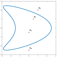
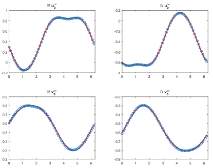
![[Uncaptioned image]](/html/1509.06268/assets/x4.png)