Leptoquark effects on $b\to s\nu\bar{\nu}$ and $B\to Kl^{+}l^{-}$ decay processes

Abstract

We study the rare semileptonic decays of $B$ mesons induced by $b\to s\nu\bar{\nu}$ as well as $b\to sl^{+}l^{-}$ transitions in the scalar leptoquark model where the leptoquarks transform as $(3,2,7/6)$ and $(3,2,1/6)$ under the standard model gauge group. The leptoquark parameter space is constrained using the most recent experimental results on ${\rm Br}(B_{s}\rightarrow\mu^{+}\mu^{-})$ and ${\rm Br}(B_{d}\to X_{s}\mu^{+}\mu^{-})$ processes. Considering only the baryon number conserving leptoquark interactions, we estimate the branching ratios for the exclusive $\bar{B}\rightarrow\bar{K}^{(*)}\nu\bar{\nu}$ and inclusive $B\rightarrow X_{s}\nu\bar{\nu}$ decay processes by using the constraint parameters. We also obtain the low recoil (large lepton invariant mass, i.e., $q^{2}\sim m^{2}_{b}$) predictions for the angular distribution of $\bar{B}\rightarrow\bar{K}l^{+}l^{-}$ process and several other observables including the flat term and lepton flavour non-universality factor in this model.

I introduction

It is well-known that the study of $B$ physics plays an important role to critically test the standard model (SM) predictions and to look for possible signature of new physics beyond it. In particular, the rare decays of $B$ mesons which are mediated by flavour changing neutral current (FCNC) transitions are well-suited for searching the effects of possible new interactions beyond the SM. This is due to the fact that the FCNC transitions $b\to s,d$ are highly suppressed in the SM as they occur only at one-loop level and hence, they are very sensitive to new physics. Recently the decay modes $B\to K^{(*)}l^{+}l^{-}$, which are mediated by the quark level transition $b\to sl^{+}l^{-}$ have attracted a lot of attention, as several anomalies at the level of few sigma are observed in the LHCb experiment lhcb1 ; lhcb2 ; lhcb7 . Furthermore, the deviation in the ratio of rates of $B\to K\mu\mu$ over $B\to Kee$ ($R_{K}$) is a hint of violation of lepton universality lhcb3 . This in turn requires the careful analyses of the angular observables for these processes both in the low and high $q^{2}$ regime.

Recently various $B$ physics experiments such as BaBar, Belle, CDF and LHCb have provided data on the angular distributions of $B\to K^{*}l^{+}l^{-}$ and $B\to Kl^{+}l^{-}$ decay processes both in the low and the large recoil region except the intermediate region around $q^{2}\sim m^{2}_{J/\psi}$ and $m^{2}_{\psi^{\prime}}$. The intermediate region is dominated by the pronounced charmonium resonance background induced by the decays $B\to K(\bar{c}c)\to Kl^{+}l^{-}$, where $\bar{c}c=J/\psi,\psi^{\prime}$. Using QCD factorization method the physical observables in the high recoil region can be calculated and the angular distribution of $\bar{B}\to\bar{K}l^{+}l^{-}$ at low recoil can be computed using simultaneous heavy quark effective theory and operator product expansions in $1/Q$, with $Q=(m_{b},\sqrt{q^{2}})$ i.e. $\sqrt{q^{2}}$ is of the order of the $b$-quark mass grinstein2 ; beylich . In this work, we are interested to study the decay process $B\to Kll$ in the region of low hadronic recoil i.e. above the $\psi^{\prime}$ peak in the scalar leptoquark (LQ) model. We have studied the $B\to K\mu^{+}\mu^{-}$ in the large recoil limit in Ref. mohanta2 and found that the various anomalies associated with the isospin asymmetry parameter and the lepton flavour non-universality factor ($R_{K}$) for this process can be explained in this model.

Similarly the rare semileptonic decays of $B$ mesons with $\nu\bar{\nu}$ pair in the final state, i.e., $B\to K^{(*)}\nu\bar{\nu}$ are also significantly suppressed in the SM and their long distance contributions are generally subleading. These decays are theoretically very clean due to the absence of photonic penguin contributions and strong suppression of light quarks. The experimental measurement of the inclusive decay rate probably be un-achievable due to the missing neutrinos, however, the exclusive channels like $B\to K^{*}\nu\bar{\nu}$ and $B\to K\nu\bar{\nu}$ are more promising as far as the measurement of branching ratios and other related observables are concerned. Theoretically, study of these decays requires calculation of relevant form factors by non-perturbative methods.

In recent times, there are many interesting papers which are contemplated to explain the anomalies associated with the $b\to sl^{+}l^{-}$ processes, observed at LHCb experiment lhcb1 ; lhcb2 ; lhcb7 ; lhcb3 , both in the context of various new physics models as well as in model independent ways matias1 ; jager ; huber ; beaujean . In this paper, we intend to study the effect of scalar leptoquarks transform as $(3,2,7/6)$ and $(3,2,1/6)$ under the standard model gauge group, on the branching ratio as well as on other asymmetry parameters in the low-recoil region of $B\to Kl^{+}l^{-}$ process. We also consider the processes $B\to K^{(*)}\nu\bar{\nu}$ and $B\to X_{s}\nu\bar{\nu}$ involving the quark level transitions $b\to s\nu\bar{\nu}$ in the full physical regime. It is well-known that leptoquarks are scalar or vector color triplet bosonic particles which make leptons couple directly to quarks and vice versa and carry both lepton as well as baryon quantum numbers and fractional electric charge. Leptoquarks can be included in the low energy theory as a relic of a more fundamental theory at some high energy scale in the extended SM georgi , such as grand unified theories georgi ; georgi2 , Pati-Salam models, models of extended technicolor schrempp and composite models kaplan . Leptoquarks are classified by their fermion number ($F=3B+L$), spin and charge. Usually they have a mass near the unification scale to avoid rapid proton decay, even so leptoquarks may exist at a mass accessible to present collider, if baryon and lepton numbers would conserve separately. The leptoquark properties and the additional new physics contribution to the SM have been very well studied in the literature davidson ; arnold ; kosnik ; mohanta2 ; mohanta1 ; leptoquark .

The plan of the paper is follows. In section II we present the effective Hamiltonian responsible for $b\rightarrow sl^{+}l^{-}$ processes. We also discuss the new physics contributions due to the exchange of scalar leptoquarks. In section III we discuss the constraints on leptoquark parameter space by using the recently measured branching ratios of the rare decay modes $B_{s}\rightarrow\mu^{+}\mu^{-}$ and $B_{d}\to X_{s}\mu^{+}\mu^{-}$. The branching ratio, the flat term and the lepton non-universality factor $(R_{K})$ for the decay mode $\bar{B}\to\bar{K}l^{+}l^{-}$, where $l=e,\mu,\tau$ at low recoil limit are computed in section IV. In section V we work out the branching ratio of $\bar{B}\to\bar{K}\nu\bar{\nu}$ process in the full kinematically accessible physical region. The branching ratio, polarization and other asymmetries in $\bar{B}\to\bar{K}^{*}\nu\bar{\nu}$ process have been computed in section VI. The inclusive decay process $B\to X_{s}\nu\bar{\nu}$ is discussed in section VII and section VIII contains the summary and conclusion.

II The Effective Hamiltonian for $b\to sl^{+}l^{-}$ process

The effective Hamiltonian describing the processes induced by the FCNC $b\rightarrow sl^{+}l^{-}$ transitions is given by buras1

$${\cal H}_{eff} = -\frac{4G_{F}}{\sqrt{2}}V_{tb}V_{ts}^{*}\Bigg{[}\sum_{i=1}^{6}C_{i}(\mu)O_{i}+\sum_{i=7,9,10}\left(C_{i}(\mu)O_{i}+C_{i}^{\prime}(\mu)O_{i}^{\prime}\right)\Bigg{]}\;,$$ (1)

which consists of the tree level current-current operators ($O_{1,2}$), QCD penguin operators ($O_{3-6}$) alongwith the magnetic $O_{7}^{(\prime)}$ and semileptonic electroweak penguin operators $O_{9,10}^{(\prime)}$. The magnetic and electroweak penguin operators can be expressed as

$$O_{7}^{(\prime)} = \frac{e}{16\pi^{2}}\Big{(}\bar{s}\sigma_{\mu\nu}(m_{s}P_{L(R)}+m_{b}P_{R(L)})b\Big{)}F^{\mu\nu}$$

$$O_{9}^{(\prime)} = \frac{\alpha}{4\pi}(\bar{s}\gamma^{\mu}P_{L(R)}b)(\bar{l}\gamma_{\mu}l)\;,~{}~{}~{}~{}~{}~{}~{}O_{10}^{(\prime)}=\frac{\alpha}{4\pi}(\bar{s}\gamma^{\mu}P_{L(R)}b)(\bar{l}\gamma_{\mu}\gamma_{5}l)\;.$$ (2)

It should be noted that the primed operators are absent in the SM. The values of Wilson coefficients $C_{i=1,\cdots,10}$, which are evaluated in the next-to-next leading order at the renormalization scale $\mu=m_{b}$ are taken from kohda . Here $V_{qq^{\prime}}$ denotes the CKM matrix element, $G_{F}$ is the Fermi constant, $\alpha$ is the fine-structure constant and $P_{L,R}=(1\mp\gamma_{5})/2$ are the chiral projectors. Due to the negligible contribution of the CKM-suppressed factor $V_{ub}V_{us}^{*}$, there is no CP violation in the decay amplitude in the SM. These processes will receive additional contributions due to the exchange of scalar leptoquarks. In particular there will be new contributions to the electroweak penguin operators $O_{9}$ and $O_{10}$ as well their right-handed counterparts $O_{9}^{\prime}$ and $O_{10}^{\prime}$. In the following subsection we will present these additional contributions to the SM effective Hamiltonian due to the exchange of such leptoquarks.

II.1 Scalar LQ Contributions to $b\to sl^{+}l^{-}$ effective Hamiltonian

There are ten different types of leptoquarks under the $SU(3)\times SU(2)\times U(1)$ gauge group ref45 , half of them have scalar nature and other halves have vector nature under the Lorentz transformation. The scalar leptoquarks have spin zero and could potentially contribute to the quark level transition $b\to sl^{+}l^{-}$. Here we would like to consider the minimal renormalizable scalar leptoquark model arnold , containing one single additional representation of $SU(3)\times SU(2)\times U(1)$, which does not allow proton decay. There are only two such models with representations under the SM gauge group as $\Delta^{(7/6)}\equiv(3,2,7/6)$ and $\Delta^{(1/6)}\equiv(3,2,1/6)$ arnold , which have sizeable Yukawa couplings to matter fields. These scalar leptoquarks do not have baryon number violation in the perturbation theory and could be light enough to be accessible in accelerator searches. The interaction Lagrangian of the scalar leptoquark $\Delta^{(7/6)}$ with the fermion bilinear is given as kosnik

$$\mathcal{L}^{(7/6)}=g_{R}\bar{Q}_{L}\Delta^{(7/6)}l_{R}+h.c.,$$ (3)

where $Q_{L}$ is the left handed quark doublet and $l_{R}$ is the right-handed charged lepton singlet. After performing the Fierz transformation and comparing with the SM effective Hamiltonian (1), one can obtain the new Wilson coefficients as discussed in Ref. kosnik

$$C_{9}^{NP}=C_{10}^{NP}=-\frac{\pi}{2\sqrt{2}G_{f}\alpha V_{tb}V_{ts}^{*}}\frac{(g_{R})_{sl}(g_{R})_{bl}^{*}}{M_{\Delta^{(7/6)}}^{2}}\;.$$ (4)

Similarly, the Lagrangian for the coupling of scalar leptoquark $\Delta^{(1/6)}$ to the SM fermions is given by

$$\mathcal{L}^{(1/6)}=g_{L}\bar{d_{R}}\tilde{\Delta}^{(1/6)\dagger}L+h.c.,\hskip 14.22636pt{\rm with}\hskip 14.22636pt\tilde{\Delta}\equiv i\tau_{2}\Delta^{*},$$ (5)

where $\tau_{2}$ is the Pauli matrix and consists of operators with right-handed quark currents. Proceeding like the previous case one can obtain the new Wilson coefficients as

$$C_{9}^{\prime NP}=-C_{10}^{\prime NP}=\frac{\pi}{2\sqrt{2}G_{f}\alpha V_{tb}V_{ts}^{*}}\frac{(g_{L})_{sl}(g_{L})_{bl}^{*}}{M_{\Delta^{(1/6)}}^{2}},$$ (6)

which are associated with the right-handed semileptonic electroweak penguin operators $O_{9}^{\prime}$ and $O_{10}^{\prime}$.

III Constraint on the LQ parameters

After having the idea of possible scalar leptoquark contributions to the $b\to sll$ processes we now proceed to constraint the LQ couplings using the theoretical bobeth1 and experimental branching ratio cms ; lhcb5 ; lhcb6 of $B_{s}\to\mu^{+}\mu^{-}$ process. This process is mediated by $b\to s\mu\mu$ transition and hence well-suited for constraining the LQ parameter space. In the SM the branching ratio for this process depends only on the Wilson coefficient $C_{10}$. However, in the scalar LQ model there will be additional contributions due to the leptoquark exchange which are characterized by the new Wilson coefficients $C_{10}^{NP}$ and $C_{10}^{{}^{\prime}NP}$ depending on the nature of the LQs. Thus, in this model the branching ratio has the form mohanta1 ; mohanta2

$${\rm Br}(B_{s}\to\mu^{+}\mu^{-})=\frac{G_{F}^{2}}{16\pi^{3}}\tau_{B_{s}}\alpha^{2}f_{B_{s}}^{2}M_{B_{s}}m_{\mu}^{2}|V_{tb}V_{ts}^{*}|^{2}\left|C_{10}^{SM}+C_{10}^{NP}-C_{10}^{{}^{\prime}NP}\right|^{2}\sqrt{1-\frac{4m_{\mu}^{2}}{M_{B_{s}}^{2}}}\;,$$ (7)

which can be expressed as

$${\rm Br}(B_{s}\to\mu^{+}\mu^{-})={\rm Br}^{SM}\left|1+\frac{C_{10}^{NP}-C_{10}^{{}^{\prime}NP}}{C_{10}^{SM}}\right|^{2}\equiv{\rm Br}^{SM}\left|1+re^{i\phi^{NP}}\right|^{2}\;,$$ (8)

where ${\rm Br}^{SM}$ is the SM branching ratio and we define the parameters $r$ and $\phi^{NP}$ as

$$re^{i\phi^{NP}}=\frac{C_{10}^{NP}-C_{10}^{{}^{\prime}NP}}{C_{10}^{SM}}\;.$$ (9)

Now comparing the SM theoretical prediction of ${\rm Br}(B_{s}\to\mu\mu)$ bobeth1

$${\rm Br}(B_{s}\to\mu^{+}\mu^{-})|_{\rm SM} = \left(3.65\pm 0.23\right)\times 10^{-9},$$ (10)

with the corresponding experimental value

$${\rm Br}(B_{s}\to\mu^{+}\mu^{-})=\left(2.9\pm 0.7\right)\times 10^{-9},$$ (11)

one can obtain the constraint on the new physics parameters $r$ and $\phi^{NP}$. The constraint on the leptoquark parameter space has been extracted in mohanta2 ; mohanta1 from this process, therefore, here we will simply quote the results. The allowed parameter space in $r-\phi^{NP}$ plane which is compatible with the $1\sigma$ range of the experimental data is $0\leq r\leq 0.1$ for the entire range of $\phi^{NP}$, i.e.,

$$0\leq r\leq 0.1\;,~{}~{}~{}~{}{\rm for}~{}~{}~{}~{}0\leq\phi^{NP}\leq 2\pi\;.$$ (12)

However, in this analysis we will use relatively mild constraint, consistent with both measurement of ${\rm Br}(B_{s}\to\mu^{+}\mu^{-})$ and ${\rm Br}(\bar{B}_{d}^{0}\to X_{s}\mu^{+}\mu^{-})$ mohanta2 as

$$0\leq r\leq 0.35\;,~{}~{}~{}~{}{\rm with}~{}~{}~{}~{}\pi/2\leq\phi^{NP}\leq 3\pi/2\;.$$ (13)

It should be noted that the use of this limited range of CP phase, i.e., ($\pi/2\leq\phi^{NP}\leq 3\pi/2$) is an assumption to have a relatively larger value of $r$. These bounds can be translated to obtain the bounds for the leptoquark couplings as

$$0\leq\frac{|(g_{R})_{s\mu}(g_{R})_{b\mu}^{*}|}{M_{\Delta}^{2}}\leq 5\times 10^{-9}~{}{\rm GeV}^{-2}~{}~{}~{}~{}{\rm for}~{}~{}~{}~{}\pi/2\leq\phi^{NP}\leq 3\pi/2\;.$$ (14)

After obtaining the bounds on leptoquark couplings, we now proceed to study the decay processes $B\to Kll$ and $B\to K^{(*)}(X_{s})\nu\bar{\nu}$ and the associated observables in the following sections.

IV $\bar{B}\rightarrow\bar{K}l^{+}l^{-}$ process in the low-recoil limit

The transition amplitude for the $B\to Kl^{+}l^{-}$ decay process can be obtained using the effective Hamiltonian presented in Eq. (1). The matrix elements of the various hadronic currents between the initial $B$ meson and the final $K$ meson can be parameterized in terms of the form factors $f_{0}$, $f_{T}$ and $f_{+}$ as bobeth2

$$\langle\bar{K}\left(k\right)|\bar{s}\gamma^{\mu}b|\bar{B}\left(p\right)\rangle=f_{+}\left(q^{2}\right)\left(p+k\right)^{\mu}+\left[f_{0}\left(q^{2}\right)-f_{+}\left(q^{2}\right)\right]\frac{m^{2}_{B}-m^{2}_{K}}{q^{2}}q^{\mu},$$ (15)

$$\langle\bar{K}\left(k\right)|\bar{s}\sigma^{\mu\nu}b|\bar{B}\left(p\right)\rangle=i\frac{f_{T}\left(q^{2}\right)}{m_{B}+m_{K}}\left[\left(p+k\right)^{\mu}q^{\nu}-q^{\mu}\left(p+k\right)^{\nu}\right],\hskip 71.13188pt$$ (16)

where $p,k$ are the four-momentum of the $B$-meson and Kaon respectively and $q=p-k$ is the four-momentum transferred to the dilepton system. Furthermore, using the QCD operator identity bobeth4 ; grinstein ; grinstein2 ,

$$i\partial^{\nu}\left(\bar{s}i\sigma_{\mu\nu}b\right)=-m_{b}\left(\bar{s}\gamma_{\mu}b\right)+i\partial_{\mu}\left(\bar{s}b\right)-2\left(\bar{s}i\overleftarrow{D}_{\mu}b\right),$$ (17)

an improved Isgur-Wise relation between $f_{T}$ and $f_{+}$ can be obtained as

$$f_{T}\left(q^{2},\mu\right)=\frac{m_{B}\left(m_{B}+m_{K}\right)}{q^{2}}\kappa\left(\mu\right)f_{+}\left(q^{2}\right)+\mathcal{O}\left(\frac{\Lambda}{m_{b}}\right),\hskip 85.35826pt$$ (18)

where strange quark mass has been neglected. Thus, one can obtain the amplitude for the $\bar{B}\rightarrow\bar{K}l^{+}l^{-}$ process in low recoil limit bobeth2 ; bobeth3 , after applying form factor relation (18) as

$${\cal A}\left(\bar{B}\rightarrow\bar{K}l^{+}l^{-}\right)=i\frac{G_{F}\alpha}{\sqrt{2}\pi}V_{tb}V^{*}_{ts}f_{+}(q^{2})[F_{V}p^{\mu}(\bar{l}\gamma_{\mu}l)+F_{A}p^{\mu}(\bar{l}\gamma_{\mu}\gamma_{5}l)+F_{P}(\bar{l}\gamma_{5}l)],$$ (19)

where

$$\begin{split}&F_{A}=C_{10}^{tot},\hskip 99.58464ptF_{V}=C_{9}^{tot}+\kappa\frac{2m_{b}m_{B}}{q^{2}}C_{7}^{eff},\\ &F_{P}=-m_{l}\left[1+\frac{m^{2}_{B}-m^{2}_{K}}{q^{2}}\left(1-\frac{f_{0}}{f_{+}}\right)\right]C_{10}^{tot}.\end{split}$$ (20)

In Eqn. (20), $C_{9}^{tot}=C_{9}^{eff}+C_{9}^{NP}+C_{9}^{{}^{\prime}NP}$ and $C_{10}^{tot}=C_{10}^{SM}+C_{10}^{NP}-C_{10}^{{}^{\prime}NP}$, where $C_{9}^{(\prime)NP}$ and $C_{10}^{(\prime)NP}$ are the new contributions to the Wilson coefficients arising due to the exchange of leptoquarks and the effective Wilson coefficients $C_{7,9}^{eff}$ are given in Ref. bobeth5 . The corresponding differential decay distributions is given by

$$\frac{d^{2}\Gamma_{l}\left[\bar{B}\rightarrow\bar{K}l^{+}l^{-}\right]}{dq^{2}d\cos{\theta}_{l}}=a_{l}\left(q^{2}\right)+c_{l}\left(q^{2}\right)\cos^{2}\theta_{l}\;,$$ (21)

where $\theta_{l}$ is the angle between the directions of $\bar{B}$ meson and the $l^{-}$, in the dilepton rest frame. The expressions for the $q^{2}$ dependent parameters $a_{l}$, $c_{l}$ are presented in Appendix A. Thus, the decay rate for the process $\bar{B}\rightarrow\bar{K}l^{+}l^{-}$ can be written as

$$\Gamma_{l}=2\int_{q^{2}_{min}}^{q^{2}_{max}}dq^{2}\left(a_{l}+\frac{1}{3}c_{l}\right).\hskip 113.81102pt$$ (22)

Another useful observable known as the flat term is defined as

$$F^{l}_{H}=\frac{2}{\Gamma_{l}}\int_{q^{2}_{min}}^{q^{2}_{max}}dq^{2}\left(a_{l}+c_{l}\right),\hskip 113.81102pt$$ (23)

where the hadronic uncertainties are reduced due to cancellation between the numerator and denominator. It should be noted that the lepton mass suppression of $(a_{l}+c_{l})$ follows as $(F^{l}_{H})^{SM}\propto m^{2}_{l}$, hence, it vanishes in the limit $m_{l}\rightarrow 0$.

After obtaining the expressions for branching ratio and the observable $F^{l}_{H}$, we now proceed for numerical estimation for $B\to Kl^{+}l^{-}$ process in the low recoil region. In our analysis we use the following parametrization for the $q^{2}$ dependence of form factors $f_{i}$ ($i=+,T,0)$ as bobeth2 ; mannel

$$f_{i}\left(s\right)=\frac{f_{i}\left(0\right)}{1-s/m^{2}_{res,i}}\Bigg{[}1+b^{i}_{1}\left(z\left(s\right)-z\left(0\right)+\frac{1}{2}\left(z\left(s\right)^{2}-z\left(0\right)^{2}\right)\right)\Bigg{]},$$ (24)

where we have used the notation $q^{2}\equiv s$. The $z(s)$ functions are given as

$$z\left(s\right)=\frac{\sqrt{\tau_{+}-s}-\sqrt{\tau_{+}-\tau_{0}}}{\sqrt{\tau_{+}-s}+\sqrt{\tau_{+}-\tau_{0}}},\hskip 28.45274pt\tau_{0}=\sqrt{\tau_{+}}\left(\sqrt{\tau_{+}}-\sqrt{\tau_{+}-\tau_{-}}\right),\hskip 28.45274pt\tau_{\pm}=\left(m_{B}\pm m_{K}\right)^{2}.$$

The values of $f_{i}(0)$ and $b_{1}^{i}$ are taken from bobeth2 .

For numerical evaluation, we have used the particle masses and the lifetimes of $B$ meson from pdg . For the CKM matrix elements, we have used the Wolfenstein parametrization with values $A=0.814^{+0.023}_{-0.024}$, $\lambda=0.22537\pm 0.00061$, $\bar{\rho}=0.117\pm 0.021$ and $\bar{\eta}=0.353\pm 0.013$ and the fine structure coupling constant $\alpha=1/137$. With these input parameters, the differential branching ratios for $\bar{B}_{d}^{0}\rightarrow\bar{K}^{0}e^{+}e^{-}$ (left panel), $\bar{B}_{d}^{0}\rightarrow\bar{K}^{0}\mu^{+}\mu^{-}$ (right panel) and $\bar{B}_{d}^{0}\rightarrow\bar{K}^{0}\tau^{+}\tau^{-}$ (lower panel) processes with respect to high $q^{2}$, both in the SM and in the leptoquark model are shown in Fig. 1 for $\Delta^{(7/6)}$ leptoquark and in Fig. 2 for $\Delta^{(1/6)}$. The grey bands in these plots correspond to the uncertainties arising in the SM due to the uncertainties associated with the CKM matrix elements and the hadronic form factors. The green bands correspond to the LQ contributions. For $B\to K\mu\mu$ process, we vary the values of the leptoquark couplings as given in Eq. (14) and for $B\to Kee$ and $B\to K\tau\tau$ processes we use the limits on the LQ couplings extracted from $B_{d}\to X_{s}e^{+}e^{-}$ and $B_{s}\to\tau^{+}\tau^{-}$ processes mohanta2 as

$$0\leq\frac{|(g_{R})_{se}(g_{R})_{be}^{*}|}{M_{\Delta}^{2}}\leq 1.0\times 10^{-8}~{}{\rm GeV}^{-2}\;,$$ (25)

and

$$0\leq\frac{|(g_{R})_{s\tau}(g_{R})_{b\tau}^{*}|}{M_{\Delta}^{2}}\leq 1.2\times 10^{-8}~{}{\rm GeV}^{-2}\;.$$ (26)

Since the leptoquark couplings are more tightly constrained in $b\to s\mu\mu$ transitions, the deviations of the branching ratios in the LQ model from the corresponding SM values are found to be small. For $B\to Kee$ and $B\to K\tau\tau$ these deviations are found to be significantly large. The bin-wise experimental values are shown in black in $B\to K\mu\mu$ process. From these figures it can be seen that the observed experimental data can be explained in the scalar LQ model but the deviation from the SM branching ratios are more in the $\Delta^{(1/6)}$ model. For the other observables in $B\to Kll$ processes we will show the results only for $\Delta^{(7/6)}$ leptoquark model. In Fig. 3, we have shown the lepton non-universality factors $R_{K}^{\mu e}$ (left panel) (i.e. the ratio of branching ratios of $\bar{B}\rightarrow\bar{K}\mu^{+}\mu^{-}$ and $\bar{B}\rightarrow\bar{K}e^{+}e^{-}$), $R_{K}^{\tau e}$ (right panel) and $R_{K}^{\tau\mu}$ (lower panel) variation with high $q^{2}$. From the figure one can see that there is significant deviations in the lepton-flavour non universality factor from their corresponding SM values in all the above three cases. The flat term for the $\bar{B}_{d}^{0}\rightarrow\bar{K}^{0}\mu^{+}\mu^{-}$ (left panel) and $\bar{B}_{d}^{0}\rightarrow\bar{K}^{0}\tau^{+}\tau^{-}$ (right panel) decay processes in the low recoil region are presented in Fig. 4 for $\Delta^{(7/6)}$. In this case there is practically no deviation in $B\to K\mu\mu$ whereas there is significant deviation in $B\to K\tau\tau$ process. The integrated branching ratios, flat terms and the lepton flavour non-universality factors for the $B\to Kll$ processes over the range $q^{2}\in[14.18,22.84]$ are given in Table I. The flat term for $B\to Ke^{+}e^{-}$ process has been found to be negligibly small ($F_{H}^{e}$ $\sim\mathcal{O}(10^{-7})$) due to tiny electron mass. In the low recoil region, the process having tau lepton in the final state has significant deviation from the SM.

The integrated branching ratio for $B^{0}\to K\mu\mu$ process in the range $q^{2}\in[15,22]~{}{\rm GeV}^{2}$ has been measured by the LHCb Collaboration lhcb1 and is given as

$${\rm Br}(B^{0}\to K^{0}\mu\mu)=(6.7\pm 1.1\pm 0.4)\times 10^{-8}\;.$$ (27)

Our predicted value in this range of $q^{2}$ is found to be

$${\rm Br}(B^{0}\to K^{0}\mu\mu) = (8.35\pm 0.5)\times 10^{-8},~{}~{}~{}~{}~{}~{}~{}~{}({\rm SM})$$ (28)

$$= (8.34-9.26)\times 10^{-8}\;.~{}~{}~{}~{}~{}~{}({\rm\Delta^{(7/6)}~{}LQ~{}model})$$

$$= (8.34-15.6)\times 10^{-8}\;.~{}~{}~{}~{}~{}~{}({\rm\Delta^{(1/6)}~{}LQ~{}model})$$

The predicted values of the branching ratios are slightly higher than the central measured value but consistent with its 1-$\sigma$ range.

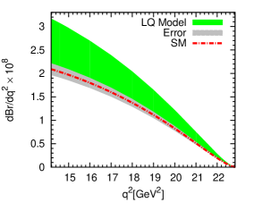
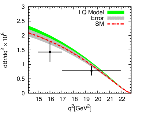
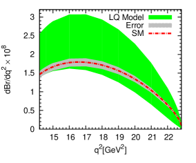
Figure 1: The variation of branching ratio for $\bar{B}_{d}^{0}\rightarrow\bar{K}^{0}e^{+}e^{-}$ (left panel), $\bar{B}\rightarrow\bar{K}\mu^{+}\mu^{-}$ (right panel) and $\bar{B}\rightarrow\bar{K}\tau^{+}\tau^{-}$ (bottom panel) with respect to high $q^{2}$ for $\Delta^{(7/6)}$ LQ. The grey bands correspond to the uncertainties arising in the SM. The $q^{2}$-averaged (bin-wise) $1-\sigma$ experimental results for $B\to K\mu\mu$ process are shown by black plots, where horizontal (vertical) line denotes the bin width ($1-\sigma$ error).

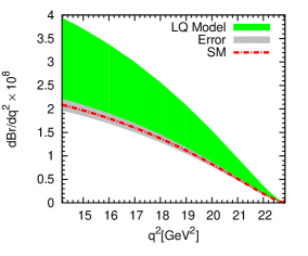
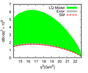
Figure 2: Same as Fig-1 for $\Delta^{(1/6)}$ LQ exhange.

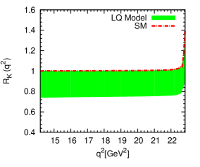
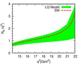
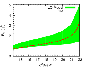
Figure 3: The variation of lepton non-universality $R_{K}^{\mu e}$ (left panel), $R_{K}^{\tau e}$ (right panel) and $R_{K}^{\tau\mu}$ (bottom panel) in low recoil region due to $\Delta^{(7/6)}$ LQ exchange.

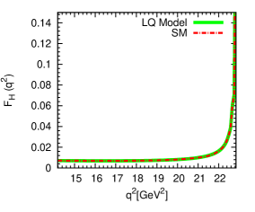
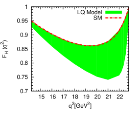
Figure 4: The variation of flat term for $\bar{B}_{d}^{0}\rightarrow\bar{K}^{0}\mu^{+}\mu^{-}$ (left panel) and $\bar{B}_{d}^{0}\rightarrow\bar{K}^{0}\tau^{+}\tau^{-}$ (right panel) with high $q^{2}$ for $\Delta^{(7/6)}$ LQ.

Oservables	SM predictions	Values in $\Delta^{(7/6)}$ LQ model	Values in $\Delta^{(1/6)}$ LQ model
Br($B_{d}^{0}\to K^{0}e^{+}e^{-}$)	$(1.005\pm 0.06)$	$(1.004-1.5)$	$(1.005-1.88)$
Br($B_{d}^{0}\to K^{0}\mu^{+}\mu^{-}$)	$(1.01\pm 0.06)$	$(1.01-1.12)$	$(1.008-1.89)$
Br($B_{d}^{0}\to K^{0}\tau^{+}\tau^{-}$)	$(1.21\pm 0.73)$	$(0.99-2.07)$	$(1.2-4.2)$
$\langle R_{K}^{\mu e}\rangle$	1.0035	$0.75-1.00$	1.0035
$\langle R_{K}^{\tau e}\rangle$	1.21	$0.98-1.85$	$(1.2-2.3)$
$\langle R_{K}^{\tau\mu}\rangle$	1.198	$0.98-1.85$	$(1.2-2.2)$
$\langle F_{H}^{e}\rangle$	$1.75\times 10^{-7}$	$(1.74-1.75)\times 10^{-7}$	$(1.73-1.75)\times 10^{-7}$
$\langle F_{H}^{\mu}\rangle$	$7.5\times 10^{-3}$	$(7.4-7.55)\times 10^{-3}$	$(7.4-7.5)\times 10^{-3}$
$\langle F_{H}^{\tau}\rangle$	0.89	0.8 - 1.38	0.88-0.89

Table 1: The predicted values for the integrated branching ratios (in units of $10^{-7}$), flat terms and lepton non-universality factors in the range $q^{2}\in[14.18,22.84]~{}{\rm GeV}^{2}$ for the $B\to Kl^{+}l^{-}$ process, $l=e,\mu,\tau$.

V $B\rightarrow K\nu\bar{\nu}$ process

The $B\rightarrow K\nu\bar{\nu}$ process is mediated by the quark level transition $b\to s\nu\bar{\nu}$ and the effective Hamiltonian describing such transition is given as buras2

$$\mathcal{H}_{eff}=\frac{-4G_{f}}{\sqrt{2}}V_{tb}V_{ts}^{*}\left(C^{\nu}_{L}\mathcal{O}^{\nu}_{L}+C^{\nu}_{R}\mathcal{O}^{\nu}_{R}\right)+h.c.,$$ (29)

where

$$\mathcal{O}^{\nu}_{L}=\frac{e^{2}}{16\pi^{2}}\left(\bar{s}\gamma_{\mu}P_{L}b\right)\left(\bar{\nu}\gamma^{\mu}\left(1-\gamma_{5}\right)\nu\right),\hskip 28.45274pt\mathcal{O}^{\nu}_{R}=\frac{e^{2}}{16\pi^{2}}\left(\bar{s}\gamma_{\mu}P_{R}b\right)\left(\bar{\nu}\gamma^{\mu}\left(1-\gamma_{5}\right)\nu\right),$$ (30)

are the dimension-six operators and $C^{\nu}_{L,R}$ are their corresponding Wilson coefficients. The coefficient $C^{\nu}_{R}$ has negligible value within the standard model while $C^{\nu}_{L}$ can be calculated by using the loop function and is given by

$$C^{\nu}_{L}=-X(x_{t})/\sin^{2}\theta_{w}\;.$$ (31)

The necessary loop functions are presented in Appendix B. The decay distribution with respect to the di-neutrino invariant mass can be expressed as fazio

$$\frac{d\Gamma}{ds_{B}}=\frac{G_{f}^{2}\alpha^{2}}{256\pi^{5}}|V_{ts}^{*}V_{tb}|^{2}m_{B}^{5}\lambda^{3/2}(s_{B},\tilde{m}_{K}^{2},1)|f_{+}^{K}(s_{B})|^{2}|C_{L}^{\nu}+C_{R}^{\nu}|^{2}.$$ (32)

where $\tilde{m}_{i}=m_{i}/m_{B}$ and $s_{B}=s/m_{B}^{2}$. The decay rate has been multiplied with an extra factor 3 due to the sum over all neutrino flavours. It should be noted that in Eq. (32) $C_{R}^{\nu}$ is the new Wilson coefficient arises due to the exchange of the leptoquark $\Delta^{(1/6)}$. In order to find out its value, we consider the new contribution to the effective Hamiltonian due to the exchange of such leptoquark which is given as

$${\cal H}_{LQ}=\frac{(g_{L})_{s\nu}(g_{L})_{b\nu}^{*}}{4M_{\Delta^{(1/6)}}^{2}}(\bar{s}\gamma^{\mu}P_{R}b)(\bar{\nu}\gamma_{\mu}(1-\gamma_{5})\nu)\;.$$ (33)

Comparing Eqs. (29) and (33), one can obtain the new Wilson coefficient as

$$C_{R}^{\nu}|_{LQ}=-\frac{\pi}{2\sqrt{2}G_{F}\alpha V_{tb}V_{ts}^{*}}\frac{(g_{L})_{s\nu}(g_{L})_{b\nu}^{*}}{M_{\Delta^{(1/6)}}^{2}}\;.$$ (34)

For numerical estimation, we use the $B\to K$ form factor $f_{+}^{K}$ evaluated in the light cone sum rule (LCSR) approach ball3 as

$$f_{+}^{K}(q^{2})=\frac{r_{1}}{1-q^{2}/m_{1}^{2}}+\frac{r_{2}}{(1-q^{2}/m_{1}^{2})^{2}}\;,$$ (35)

which is valid in the full physical region. Furthermore, in contrast to $B\to Kl^{+}l^{-}$ process, which has dominant charmonium resonance background from $B\to K(J/\psi)\to Kl^{+}l^{-}$, there are no such analogous long-distance QCD contributions in this case as there are no intermediate states which can decay into two neutrinos. For the $b\to s\nu\bar{\nu}$ LQ couplings we use the values as we used for $b\to s\mu\mu$ as these two processes are related by $SU(2)_{L}$ symmetry. The variation of branching ratio with respect to $s_{B}$ in the full physical regime $0\leqslant s_{B}\leqslant(1-\tilde{m}_{K})^{2}$ is shown in Fig. 5 and the predicted branching ratio is given in Table II, which is well below the present upper limit ${\rm Br}(B_{d}^{0}\to K\nu\bar{\nu})<4.9\times 10^{-5}$ pdg .

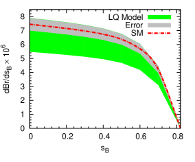
Figure 5: The variation of branching ratio of $B\rightarrow K\nu\bar{\nu}$ with respect to the normalized invariant masses squared $s_{B}$ in the SM and $\Delta^{(1/6)}$ LQ model. The grey band corresponds to the uncertainties arising in the SM.

VI $B\to K^{*}\nu\bar{\nu}$ process

The study of $B\to K^{*}\nu\bar{\nu}$ is also quite important as this process is related to $B\to K^{*}\mu\mu$ process by $SU(2)_{L}$ and therefore, the recent LHCb anomalies in $B\to K^{*}\mu\mu$ would in principle also show up in $B\to K^{*}\nu\nu$. The experimental information about this exclusive decay process can be described by the double differential decay distribution. In order to compute the decay rate, we must have the idea about the matrix element of the effective Hamiltonian (29) between the initial $B$ meson and the final particles. Due to the non-detection of the two neutrinos, experimentally we can’t distinguish between the transverse polarization, so the decay rate will be the addition of both longitudinal and transverse polarizations. The double differential decay rate with respect to $s_{B}$ and $\cos\theta$ is given by buras2 ; kim

$$\frac{d^{2}\Gamma}{ds_{B}d\cos\theta}=\frac{3}{4}\frac{d\Gamma_{T}}{ds_{B}}\sin^{2}\theta+\frac{3}{2}\frac{d\Gamma_{L}}{ds_{B}}\cos^{2}\theta,$$ (36)

where the longitudinal and transverse decay rate are

$$\frac{d\Gamma_{L}}{ds_{B}}=3m_{B}^{2}|A_{0}|^{2},\hskip 56.9055pt\frac{d\Gamma_{T}}{ds_{B}}=3m_{B}^{2}(|A_{\perp}|^{2}+|A_{\parallel}|^{2}).$$ (37)

The transversality amplitudes $A_{\perp,\parallel,0}$ in terms of the form factors and Wilson coefficients are listed in Appendix C.

The fractions of $K^{*}$ longitudinal and transverse polarizations are given as

$$F_{L,T}=\frac{d\Gamma_{L,T}/ds_{B}}{d\Gamma/ds_{B}},$$ (38)

and the $K^{*}$ polarization factor is

$$\alpha_{K^{*}}=\frac{2F_{L}}{F_{T}}-1.$$ (39)

The transverse asymmetry parameters are given as egede ; simula

$$A_{T}^{(1)}=\frac{-2Re(A_{\perp}A_{\parallel}^{*})}{|A_{\perp}|^{2}+|A_{\parallel}|^{2}}\;,~{}~{}~{}~{}~{}~{}~{}~{}A_{T}^{(2)}=\frac{|A_{\perp}|^{2}-|A_{\parallel}|^{2}}{|A_{\perp}|^{2}+|A_{\parallel}|^{2}}.$$ (40)

However, one can’t extract $A_{T}^{(1)}$ from the full angular distribution of $B\rightarrow K^{*}\nu\bar{\nu}$, as it is not invariant under the symmetry of the distribution function and requires measurement of the neutrino polarization. So it can’t be measured experimentally at $B$ factories or in LHCb. The transverse asymmetry $A_{T}^{(2)}$ is theoretically clean and could be measurable in Belle-II.

For numerical evaluation we use the $q^{2}$ dependence of the $B\to K^{*}$ form factors $V(q^{2}),~{}A_{1}(q_{2}),~{}A_{2}(q^{2})$ from ball1 ; ball2 . The variation of the branching ratio of $B\rightarrow K^{*}\nu\bar{\nu}$ with respect to the neutrino invariant mass, $s_{B}$ is shown in Fig. 6. Fig. 7 contains the longitudinal and transverse polarizations of $K^{*}$ verses $s_{B}$. The polarization factor and the transverse asymmetry variation with respect to $s_{B}$ in the full region are shown in Fig. 8. Although there is certain deviation found between the SM and LQ model predictions for the branching fraction, but no such noticeable deviations found between the SM and LQ predictions for the longitudinal/transverse polarizations, transverse asymmetry parameters $A_{T}^{(2)}$. The integrated values of branching ratio over the range $s_{B}\in[0,0.69]$ are presented in Table II, which are well below the the present upper limit ${\rm Br}(B_{d}^{0}\to K^{*}\nu\bar{\nu})<5.5\times 10^{-5}$ pdg .

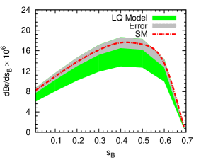
Figure 6: The variation of branching ratio of $B\rightarrow K^{*}\nu\bar{\nu}$ with respect to the $s_{B}$ in the SM and $\Delta^{(1/6)}$ LQ model. The grey band corresponds to the uncertainties arising in the SM.

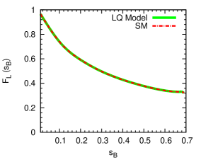
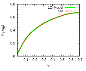
Figure 7: The variation of longitudinal (left panel) and transverse (right panel) polarization of $K^{*}$ with $s_{B}$.

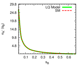
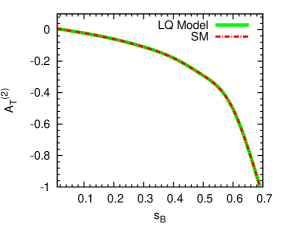
Figure 8: The variation of $K^{*}$ polarization factor (left panel) and the transverse asymmetry (right panel) with respect to $s_{B}$.

VII $B\to X_{s}\nu\bar{\nu}$

The inclusive decay $B\to X_{s}\nu\bar{\nu}$ is dominated by the $Z$-exchange and can be searched through the large missing energy associated with the two neutrinos. This decay mode is theoretically very clean, since both the perturbative $\alpha_{s}$ and the non-perturbative corrections are small. So these decays do not suffer from the form factor uncertainties and thus, are very sensitive to the search for new physics beyond the SM. The decay distribution with respect to $s_{b}=s/m_{b}^{2}$ can be written as

$$\frac{d\Gamma}{ds_{b}} = m_{b}^{5}\frac{\alpha^{2}G_{f}^{2}}{128\pi^{5}}|V_{ts}^{*}V_{tb}|^{2}\kappa(0)(|C_{L}^{\nu}|^{2}+|C_{R}^{\nu}|^{2})\lambda^{1/2}(1,\tilde{m}_{s}^{2},s_{b})$$ (41)

$$\times \left[3s_{b}(1+\tilde{m}_{s}^{2}-s_{b}-4\tilde{m}_{s}\frac{Re(C_{L}^{\nu}C_{R}^{\nu*})}{|C_{L}^{\nu}|^{2}+|C_{R}^{\nu}|^{2}})+\lambda(1,\tilde{m}_{s}^{2},s_{b})\right]$$

where $\tilde{m}_{i}=m_{i}/m_{b}$ and $\kappa(0)=0.83$ is the QCD correction to the $b\to s\nu\bar{\nu}$ matrix element nardi . The full kinematically accessible physical region is $0\leq s_{b}\leq(1-\tilde{m}_{s})^{2}$. In Fig. 9, we have shown the variation of the branching ratio with respect to $s_{b}$ and the integrated branching ratio values over the range $s_{b}\in[0,0.96]$ both in the SM and in the leptoquark model are presented in Table II.

We define the ratio of branching ratios as fazio ,

$$R_{K}=\frac{{\rm Br}(B\to K\nu\bar{\nu})}{{\rm Br}(B\to X_{s}\nu\bar{\nu})},$$ (42)

and

$$R_{K^{*}}=\frac{{\rm Br}(B\to K^{*}\nu\bar{\nu})}{{\rm Br}(B\to X_{s}\nu\bar{\nu})}$$ (43)

and the variation of $R_{K}$ and $R_{K^{*}}$ with respect to $s_{B}$ in the full kinematically allowed region is shown in Fig. 10. In this case also no deviation found between the SM and leptoquark predictions.

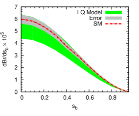
Figure 9: The variation of branching ratio of $B\rightarrow X_{s}\nu\bar{\nu}$ with respect to the $s_{b}$.

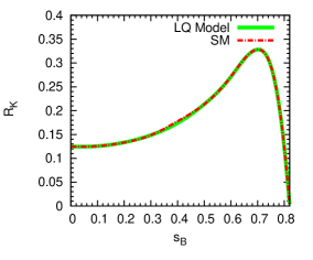
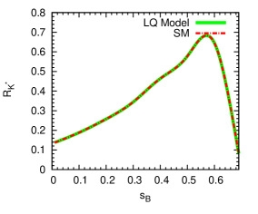
Figure 10: The variation of $R_{K}$ (left panel) and $R_{K^{*}}$ (right panel) with respect to $s_{B}$.

Observables	SM prediction	Values in $\Delta^{(1/6)}$ LQ model
Br($B_{d}^{0}\to K^{0}\nu\bar{\nu}$)	$(4.9\pm 0.29)\times 10^{-6}$	$(3.6-5.2)\times 10^{-6}$
Br($B_{d}^{0}\to K^{*}\nu\bar{\nu}$)	$(9.54\pm 0.57)\times 10^{-6}$	$(7.02-10.13)\times 10^{-6}$
Br($B\to X_{s}\nu\bar{\nu}$)	$(2.98\pm 0.18)\times 10^{-5}$	$(2.2-3.17)\times 10^{-5}$
$R_{K}$	0.164	$(0.163-0.164)$
$R_{K^{*}}$	0.32	0.32

Table 2: The predicted branching ratios for $B\to{(K,K^{*},X_{s})}\nu\bar{\nu}$ processes and $R_{K,K^{*}}$ for $B\to X_{s}\nu\bar{\nu}$ in their respective full physical ranges.

VIII conclusion

In this paper we have studied the effect of scalar leptoquarks on the rare semileptonic decays of $B$ meson. In particular, we focus on the decay processes $B\to Kl^{+}l^{-}$ in low recoil limit and the di-neutrino decay channels $B\to K^{(*)}(X_{s})\nu\bar{\nu}$. The leptoquark parameter space is constrained by considering the recently measured branching ratios of $B_{s}\to\mu^{+}\mu^{-}$ and $B_{d}\to X_{s}\mu^{+}\mu^{-}$ processes. Using the allowed parameter space we predicted the branching ratio, lepton non-universality factors and the flat terms for the $B\to Kl^{+}l^{-}$ process in the low recoil region. We found that the measured branching ratio can be accommodated in the scalar leptoquark model. We have also calculated the branching ratios of $B\to K^{(*)}\nu\bar{\nu}$ and $B\to X_{s}\nu\bar{\nu}$ processes. The predicted branching ratios for $B\to K^{(*)}\nu\bar{\nu}$ processes are well below the present upper limits. The polarization of $K^{*}$ and transverse asymmetry for $B\to K^{*}\nu\bar{\nu}$ are also computed using the constraint leptoquark parameters. However, we found no deviation between the SM prediction and the LQ results for different polarization variables and the transverse asymmetry parameter.

Acknowledgments

We would like to thank Science and Engineering Research Board (SERB), Government of India for financial support through grant No. SB/S2/HEP-017/2015.

Appendix A $a_{l}$ and $c_{l}$ functions in $B\to Kll$ process

The $a_{l}$ and $c_{l}$ parameters in the decay distribution of the $B\to Kl^{+}l^{-}$ processes (21) can be expressed as

$$\frac{a_{l}}{\Gamma_{0}\sqrt{\lambda}\beta_{l}f^{2}_{+}} = \frac{\lambda}{4}\left(|F_{A}|^{2}+|F_{V}|^{2}\right)+2m_{l}\left(m^{2}_{B}-m^{2}_{K}+q^{2}\right)Re\left(F_{P}F^{*}_{A}\right)$$ (44)

$$+ 4m_{l}^{2}m^{2}_{B}{|F_{A}|}^{2}+q^{2}{|F_{P}|}^{2},$$

$$\frac{c_{l}}{\Gamma_{0}\sqrt{\lambda}\beta_{l}f^{2}_{+}}=-\beta^{2}_{l}\frac{\lambda}{4}\left(|F_{A}|^{2}+|F_{V}|^{2}\right),\hskip 156.49014pt$$ (45)

with

$$\Gamma_{0}=\frac{G^{2}_{F}\alpha^{2}|V_{tb}V^{*}_{ts}|^{2}}{2^{9}\pi^{5}m^{3}_{B}},\hskip 71.13188pt\beta_{l}=\sqrt{1-\frac{4m_{l}^{2}}{q^{2}}},\hskip 79.6678pt$$ (46)

and

$$\lambda=m_{B}^{4}+m_{K}^{4}+q^{4}-2\left(m_{B}^{2}m_{K}^{2}+m_{B}^{2}q^{2}+m_{K}^{2}q^{2}\right).$$

Appendix B Loop functions

The loop function $X(x_{t})$ in Eq. (31), including correction ${\cal O}(\alpha_{s})$ at the next-to-leading order in QCD, is given by misiak ; buchalla

$$X(x_{t})=X_{0}(x_{t})+\frac{\alpha_{s}}{4\pi}X_{1}(x_{t}),$$ (47)

where

$$X_{0}(x_{t})=\frac{x_{t}}{8}\left[-\frac{2+x_{t}}{1-x_{t}}+\frac{3x_{t}-6}{(1-x_{t})^{2}}\ln x_{t}\right],$$ (48)

and

$$X_{1}(x_{t}) = -\frac{29x_{t}-x_{t}^{2}-4x_{t}^{3}}{3(1-x_{t})^{2}}-\frac{x_{t}+9x_{t}^{2}-x_{t}^{3}-x_{t}^{4}}{(1-x_{t})^{3}}\ln x_{t}$$ (49)

$$+ \frac{8x_{t}+4x_{t}^{2}+x_{t}^{3}-x_{t}^{4}}{2(1-x_{t})^{3}}\ln^{2}x_{t}-\frac{4x_{t}-x_{t}^{3}}{(1-x_{t})^{2}}L_{2}(1-x_{t})+8x_{t}\frac{\partial X_{0}(x_{t})}{\partial x_{t}}\ln x_{\mu}.$$

In Eqs. (47-49), the parameters used are defined as $x_{t}=m_{t}^{2}/m_{W}^{2}$, $x_{\mu}=\mu^{2}/m_{W}^{2}$ with $\mu=\mathcal{O}(m_{t})$ and $L_{2}(1-x_{t})=\int_{1}^{x_{t}}dt\frac{\ln t}{1-t}$.

Appendix C Transversity amplitudes for $B\to K^{*}\nu\bar{\nu}$ process

The transversality amplitudes $A_{\perp,\parallel,0}$ for $B\to K^{*}\nu\bar{\nu}$ process are given as

$$A_{\perp}(s_{B})=2N\sqrt{2}\lambda^{1/2}(1,\tilde{m}_{K*}^{2},s_{B})(C_{L}^{\nu}+C_{R}^{\nu})\frac{V(s_{B})}{(1+\tilde{m}_{K^{*}})},\hskip 136.5733pt$$ (50)

$$A_{\parallel}(s_{B})=-2N\sqrt{2}(1+\tilde{m}_{K^{*}})(C_{L}^{\nu}-C_{R}^{\nu})A_{1}(s_{B}),\hskip 176.407pt$$ (51)

$$A_{0}(s_{B})=-\frac{N(C_{L}^{\nu}-C_{R}^{\nu})}{\tilde{m}_{K^{*}}\sqrt{s_{B}}}\left[(1-\tilde{m}_{K^{*}}^{2}-s_{B})(1+\tilde{m}_{K^{*}})A_{1}(s_{B})-\lambda(1,\tilde{m}_{K^{*}}^{2},s_{B})\frac{A_{2}(s_{B})}{1+\tilde{m}_{K^{*}}}\right],$$ (52)

with

$$N=V_{tb}V_{ts}^{*}\left[\frac{G_{f}^{2}\alpha^{2}m_{B}^{3}}{3\cdot 2^{10}\pi^{5}}s_{B}\lambda^{1/2}(1,\tilde{m}_{K^{*}}^{2},s_{B})\right]^{1/2}.$$ (53)

The various form factors $V(s_{B})$, $A_{1}(s_{B})$, $A_{2}(s_{B})$ associated with $B\to K^{*}$ transition in Eqs. (C1-C3) are defined as

$$\langle K^{*}\left(p_{K^{*}}\right)|\bar{s}\gamma_{\mu}P_{L,R}b|B\left(p\right)\rangle=i\epsilon_{\mu\nu\alpha\beta}\epsilon^{\nu*}p^{\alpha}q^{\beta}\frac{V(s_{B})}{m_{B}+m_{K^{*}}}\mp\frac{1}{2}\Bigg{(}(m_{B}+m_{K^{*}})\epsilon^{*}_{\mu}A_{1}(s_{B})$$

$$-(\epsilon^{*}\cdotp q)(2p-q)_{\mu}\frac{A_{2}(s_{B})}{m_{B}+m_{K^{*}}}-\frac{2m_{K^{*}}}{s}(\epsilon^{*}\cdotp q)\left[A_{3}(s_{B})-A_{0}(s_{B})\right]q_{\mu}\Bigg{)},$$ (54)

where $q=p_{l^{+}}+p_{l^{-}}$ and $\epsilon^{\mu}$ is the polarization vector of $K^{*}$.

References

- (1) R. Aaij et al., [LHCb Collaboration], JHEP 1406, 133 (2014) [arXiv:1403.8044].
- (2) R. Aaij et al., [LHCb Collaboration], Phys. Rev. Lett. 111, 191801 (2013) [arXiv:1308.1707].
- (3) R. Aaij et al., [LHCb Collaboration], JHEP 07, 133 (2012) [arXiv:1205.3422].
- (4) R. Aaij et al., [LHCb Collaboration], Phys. Rev. Lett. 113, 151601 (2014) [arXiv:1406.6482].
- (5) B. Grinstein and Dan Pirjol, Phys. Rev. D 70, 114005 (2004) [arXiv:hep-ph/0404250].
- (6) M. Beylich, G. Buchalla and T. Feldmann, Eur. Phys. J. C 71, 1635 (2011) [arXiv: hep-ph/1101.5118]; G. Buchalla and G. Isidori, Nucl. Phys. B 525, 333 (1998) [arXiv: hep-ph/9801456].
- (7) S. Sahoo and R. Mohanta, Phys. Rev. D 91, 094019 (2015) [arXiv:1501.05193].
- (8) S. Descotes-Genon, J. Matias, M. Ramon, J. Virto, JHEP 1301, 048 (2013) [arXiv:1207.2753].
- (9) S. Jäger, J. Martin Camalich, JHEP 05, 043 (2013) [arXiv:1212.2263]; S.Descotes-Genon, L. Hofer, J. Matias and J. Virto, JHEP 1412, 125 (2014) [arXiv:1407.8526]; S. Jäger and J. Martin Camalich [arXiv:1412.3183].
- (10) T. Huber, T. Hurth and E. Lunghi, Nucl. Phys. B 802, 40 (2008) [arXiv:0712.3009].
- (11) F. Beaujean, C. Bobeth and D. van Dyk, Eur. Phys. J. C 74, 2897 (2014) [arXiv:1310.2478]; T. Hurth and F. Mahmoudi, JHEP 04, 097 (2014) [arXiv:1312.5267];. W. Altmannshofer, S.Gori, M. Pospelov and I. Yavin, Phys. Rev. D 89, 095033 (2014) [arXiv:1403.1269]; R. Gauld, F. Goertz, and U. Haisch, JHEP 01, 069 (2014) [arXiv:1310.1082]; R. Gauld, F. Goertz and U. Haisch, Phys. Rev. D 89, 015005 (2014) [arXiv:1308.1959]; A. Datta, M. Duraisamy and D. Ghosh, Phys. Rev. D 89, 071501 (2014) [arXiv:1310.1937]; A. J. Buras and J. Girrbach, JHEP 12, 009 (2013) [arXiv:1309.2466]; A. J. Buras, F. De Fazio and J. Girrbach, JHEP 02, 112 (2014) [arXiv:1311.6729]; S. Descotes-Genon, J. Matias and J. Virto, Phys. Rev. D 88, 074002 (2013) [arXiv:1307.5683]; R. R. Horgan, Z. Liu, S. Meinel and M. Wingate, Phys. Rev. Lett. 112, 212003 (2014) [arXiv:1310.3887]; A. J. Buras, J. Girrbach-Noe, C. Niehof and D. M. Straub, JHEP 02, 184 (2015) [arXiv:1409.4557]; A. Crivellin, arXiv: 1409.0922; D. Ghosh, M. Nardecchia and S. Renner, JHEP 12, 131 (2014) [arXiv:1408.4097]; S. Biswas, D. Chowdhury, S. Han, and S. J. Lee, JHEP 02, 142 (2015) [arXiv:1409.0882]; G. Hiller and M. Schmaltz, Phys. Rev. D 90, 054014 (2014) [arXiv:1408.1627]; T. Hurth, F. Mahmoudi and S. Neshatpour, JHEP 12, 053 (2014) [arXiv:1410.4545]; S. L. Glashow, D. Guadagnoli, Kenneth Lane, Phys. Rev. Lett. 114, 091801 (2014) [arXiv:1411.0565 [hep-ph]]; D. Aristizabal Sierra, F. Staub and A. Vicente, Phys. Rev. D 92, 015001 (2015) [arXiv:1503.06077]; S. M. Boucenna, J. W. F. Valle and A. Vicente, Phys. Lett. B 750, 367 (2015) [arXiv:1503.07099]; F. Mahmoudi, S. Neshatpour, J. Virto, Eur. Phys. J. C 74, 2927, (2014) [arXiv:1401.2145]; A. Crivellin, G. D’Ambrasio, J. Heeck, Phys. Rev. Lett. 114, 151801 (2015) [arXiv:1501.00993]; A. Crivellin, G. D’Ambrasio, J. Heeck, Phys. Rev. D 91, 075006 (2015) [arXiv:1503.03477]; A. Crivellin, L. Hofer, J. Matias, U. Nierste, S. Pokorski, J. Rosiek, Phys. Rev. D 92, 054013 (2015) [arXiv:1504.07928]; D. Becirevic, S. Faster, N. Kosnik, Phys. Rev. D 92, 014016 (2015) [arXiv:1503.09024 [hep-hp]]; X.-W. Kang, B. Kubis, C. Hanhart, Ulf-G. Meibner, Phys Rev. D 89, 053015 (2014), [arXiv:1312.1193]; J. Lyon, R. Zwicky, [arXiv:1406:0566]; J. Gratex, M. Hopfer, R. Zwicky, [arXiv: 1506.03970]; R. Alonso, B. Grinstein and J. M. Camalich, Phys. Rev. Lett. 113, 241802 (2014) [arXiv:1407.7044]; R. Alonso, B. Grinstein and J. M. Camalich, JHEP 10, 184 (2015) [arXiv:1505.05164]; B. Gripaios, M. Nardecchia and S. A. Renner, JHEP 1505, 006 (2015) [arXiv:1412.1791]; A. Falkowski, M. Nardecchia, Robert Ziegler, JHEP 11, 173 (2015) [arXiv:1509.01249]; B. Gripaios, M. Nardecchia, S. A. Renner, [arXiv:1509.05020].
- (12) H. Georgi and S. L. Glashow, Phys. Rev. Lett.32, 438 (1974); J. C. Pati and A. Salam, Phys.Rev. D 10, 275 (1974).
- (13) H. Georgi, AIP Conf. Proc. 23 575 (1975); H. Fritzsch and P. Minkowski, Annals Phys. 93, 193 (1975); P. Langacker, Phys. Rep. 72, 185 (1981).
- (14) B. Schrempp and F. Shrempp, Phys. Lett. B 153, 101 (1985).
- (15) D. B. Kaplan, Nucl. Phys. B 365, 259 (1991); B. Gripaios, JHEP 1002, 045 (2010) [arXiv:0910.1789].
- (16) S. Davidson, D. C. Bailey and B. A. Campbell, Z. Phys. C 61, 613 (1994), hep-ph/9309310; I. Dorsner, S. Fajfer, J. F. Kamenik, N. Kosnik, Phys. Lett. B 682, 67 (2009) [arXiv:0906.5585]; S. Fajfer, N. Kosnik, Phys. Rev. D 79, 017502 (2009) [arXiv:0810.4858]; R. Benbrik, M. Chabab, G. Faisel, [arXiv:1009.3886]; A. V. Povarov, A. D. Smirnov, [arXiv:1010.5707]; J. P Saha, B. Misra and A. Kundu, Phys. Rev.D 81, 095011 (2010), [arXiv:1003.1384]; I. Dorsner, J. Drobnak, S. Fajfer, J. F. Kamenik, N. Kosnik, JHEP 11, 002 (2011), [arXiv: 1107.5393]; F. S. Queiroz, K. Sinha, A. Strumia, Phys. Rev. D 91, 035006 (2015) [arXiv:1409.6301]; B. Allanach, A. Alves, F. S. Queiroz, K. Sinha, A. Strumia, Phys. Rev. D 92, 055023 (2015) [arXiv:1501.03494]; L. Calibbi, A. Crivellin, T. Ota, Phys. Rev. Lett.115, 181801 (2015) [arXiv:1506.02661]; Ivo de M. Varzielas and G. Hiller, JHEP 1506, 072 (2005) [arXiv:1503.01084]; S. Sahoo and R. Mohanta, [arXiv:1507.02070].
- (17) J. M. Arnold, B. Fornal and M. B. Wise, Phys. Rev. D 88, 035009 (2013), [arXiv:1304.6119].
- (18) N. Kosnik, Phys. Rev. D 86, 055004 (2012), [arXiv:1206.2970].
- (19) R. Mohanta, Phys. Rev. D 89, 014020 (2014) [arXiv:1310.0713].
- (20) D. Aristizabal Sierra, M. Hirsch, S. G. Kovalenko, Phys. Rev. D 77, 055011 (2008), [arXiv:0710.5699]; K. S. Babu, J. Julio, Nucl. Phys. B 841, 130 (2010), [arXiv:1006.1092]; S. Davidson, S. Descotes-Genon, JHEP 1011, 073 (2010), [arXiv:1009.1998]; S. Fajfer, J. F. Kamenik, I. Nisandzic, J. Zupan, Phys. Rev. Lett. 109, 161801, (2012), [arXiv:1206.1872]; K. Cheung, W.-Y. Keung, P.-Y. Tseng, [arXiv:1508.01897]; D. A. Camargo, [arXiv:1509.04263]; S. Baek, K. Nishiwaki, [arXiv:1509.07410].
- (21) C. Bobeth, M. Misiak and J. Urban, Nucl. Phys. B 574, 291 (2000) [hep-ph/9910220]; C. Bobeth, A. J. Buras, F. Krüger and J. Urban, Nucl. Phys. B 630, 87 (2002) [hep-ph/0112305].
- (22) W.-S. Hou, M. Kohda and F. Xu, Phys. Rev. D 90, 013002 (2014) [arXiv:1403.7410].
- (23) W. Buchmuller, R. Ruckl and D. Wyler, Phys. Lett. B 191, 442 (1987); Erratum-ibid. B 448, 320 (1997).
- (24) C. Bobeth, M. Gorbahn, T. Hermann, M. Misiak, E. Stamou, M. Steinhauser, Phys. Rev. Lett. 112, 101801 (2014) [arXiv:1311.0903].
- (25) S. Chatrchyan et al., [CMS Collaboration], Phys. Rev. Lett.111, 101805 (2013), [arXiv:1307.5025].
- (26) R. Aaij et al., [LHCb Collaboration], Phys. Rev. Lett. 111, 101805 (2013), [arXiv:1307.5024].
- (27) CMS and LHCb Collaborations, EPS-HEP 2013 European Physical Society Conference on High Energy Physics, Stockholm, Sweden, 2013, Conference Report No. CMS-PAS-BPH-13-007, LHCb-CONF-2013-012, http://cds.cern.ch/record/1564324.
- (28) C. Bobeth, G. Hiller, D. van Dyk and C. Wacker, JHEP 1201, 107 (2012) [arXiv:1111.2558].
- (29) C. Bobeth, G. Hiller and D. van Dyk, JHEP 1007, 098 (2010) [arXiv:1006.5013].
- (30) B. Grinstein and D. Pirjol, Phys. Lett. B 533, 8 (2002) [arXiv:hep-ph/0201298].
- (31) C. Bobeth, G. Hiller and G. Piranishvili, JHEP 0712, 040 (2007) [arXiv:0709.4174].
- (32) C. Bobeth, G. Hiller and D. van Dyk, JHEP 1107, 067 (2011) [arXiv:1105.0376].
- (33) A. Khodjamirian, T. Mannel, A. A. Pivovarov and Y. M. Wang, JHEP 1009, 089 (2010) [arXiv:1006.4945].
- (34) K.A. Olive et al. (Particle Data Group), Chin. Phys. C 38, 090001 (2014).
- (35) W. Altmannshofer, A. J. Buras, D.M. Straub and M. Wick, JHEP 0904, 022 (2009) [arXiv:0902.0160].
- (36) P. Colangelo, F. De Fazio, P. Santorelli, and E. Scrimieri, Phys. Lett. B 395, 339 (1997) [arXiv: hep-ph/9610297].
- (37) P. Ball and R. Zwicky, Phys. Rev.D 71, 014015 (2005) [arXiv: hep-ph/0406232].
- (38) C. S. Kim, Y. G. Kim and T. Morozumi, Phys.Rev.D 60, 094007 (1999) [arXiv: hep-ph/9905528].
- (39) U. Egede, T. Hurth, J. Matias, M. Ramon, W. Reece, JHEP 11, 032 (2008) [arXiv: 0807.2589].
- (40) D. Melikhov, N. Nikitin and S. Simula, Phys. Lett. B 428, 171 (1998) [arXiv: hep-ph/9803269].
- (41) W. Altmannshofer, P. Ball, A. Barucha, A. J. Buras, D. M. Straub and M. Wick, JHEP 01, 019 (2009) [arXiv:0811.1214].
- (42) P. Ball and R. Zwicky, Phys. Rev. D 71, 014029 (2005) [arXiv: hep-ph/0412079].
- (43) Y. Grossman, Z. Ligeti and E. Nardi, Nucl. Phys.B 465, 369 (1996) [arXiv: hep-ph/9510378]; C. Bobeth, A. J. Buras, F. Kruger and J. Urban, Nucl. Phys. B 630, 87 (2002) [arXiv: hep-ph/0112305]; G. Buchalla, A.J. Buras and M. E. Lautenbacher, Rev. Mod. Phys. 68, 1125 (1996) [arXiv: hep-ph/9512380].
- (44) M. Misiak and J. Urban, Phys. Lett. B 451, 161 (1999) [arXiv: hep-ph/9901278].
- (45) G. Buchalla and A. J. Buras, Nucl. Phys. B 548, 309 (1999) [arXiv:hep-ph/9901288].