Entropy production of a Brownian ellipsoid in the overdamped limit

Abstract

We analyze the translational and rotational motion of an ellipsoidal Brownian particle from the viewpoint of stochastic thermodynamics. The particle’s Brownian motion is driven by external forces and torques and takes place in an heterogeneous thermal environment where friction coefficients and (local) temperature depend on space and time. Our analysis of the particle’s stochastic thermodynamics is based on the entropy production associated with single particle trajectories. It is motivated by the recent discovery that the overdamped limit of vanishing inertia effects (as compared to viscous fricion) produces a so-called “anomalous” contribution to the entropy production, which has no counterpart in the overdamped approximation, when inertia effects are simply discarded. Here, we show that rotational Brownian motion in the overdamped limit generates an additional contribution to the “anomalous” entropy. We calculate its specific form by performing a systematic singular perturbation analysis for the generating function of the entropy production. As a side result, we also obtain the (well-known) equations of motion in the overdamped limit. We furthermore investigate the effects of particle shape and give explicit expressions of the “anomalous entropy” for prolate and oblate spheroids and for near-spherical Brownian particles.

I Introduction

The theory of Brownian motion mazo02 ; duplantier05 ; frey05 , developed in different formulations by Einstein einstein05 , Smoluchowski smoluchowski06 and Langevin langevin06 around 1905 and 1906, describes the dynamics of a particle suspended in a fluid. A prototypical example is a small colloidal object, e.g. a polystyrene bead about a micrometer in size, floating in water at room temperature. Even without the action of externally applied forces, the particle is in an animated and erratic state of motion, generated on microscopic scales by collisions with the water molecules and visible on mesoscopic scales as irregular diffusive movement. Based upon the works mentioned above, this Brownian motion is most successfully modelled (on the mesoscopic scales) by stochastic differential equations gardiner83 ; vankampen87 ; snook07 , augmenting the Newtonian equations of motion for the particle by the forces from the surrounding liquid, namely Stokesian friction proportional to the particle velocity and thermal fluctuations related to the fluid temperature. Both originating from the surrounding fluid bath as their source, the strengths of these two forces are related by the fluctuation-dissipation theorem einstein05 ; gardiner83 ; vankampen87 .

Typically, this set of equations of motion for particle position and velocity can be simplified by adopting the so-called overdamped approximation, where one completely neglects inertia effects in the particle dynamics. This procedure is justified because for micrometer-sized objects suspended in water friction forces are by orders of magnitude larger than inertial forces purcell77 ; dusenbery11 , so that on time- and length-scales accessible under typical experimental conditions only the overdamped behavior is observable. Indeed, it takes a delicate experimental effort to actually measure the velocity of a micrometer-sized Brownian particle in a liquid huang11 ; kheifets14 .

In recent years it has been demonstrated that the stochastic equations of motion not only describe the irregular particle dynamics to high accuracy, but are also a valid starting point for a consistent theory of thermodynamic quantities which are associated with the particle movement, such as heat, work or entropy production jarzynski08 ; jarzynski11 ; seifert12 ; vandenBroeck15 , even if the particle is driven away from thermal equilibrium conditions with the heat bath. In this newly emerging field called stochastic thermodynamics, central results of surprising generality have been discovered in form of fluctuation relations; a recent summary is provided in seifert12 . The entropy production (rate) plays a particularly important role, because it constitutes a measure of irreversibility by relating probabilities of particle trajectories to their time-reversed counterparts chetrite08 .

In the present context of a colloidal particle whose stochastic dynamics is well-described by overdamped equations of motion, the fact that the definition of such a central concept as entropy production (rate) is based on single trajectories immediately raises the question of how neglecting the velocity degrees of freedom may affect the particle’s stochastic thermodynamics. Investigating this question, it has been shown in celani12 that the overdamped approximation does not fully capture the entropy production rate if the thermal environment is inhomogeneous (but in equilibrium locally). Rather, there is a contribution to the entropy production in addition to those predicted from the overdamped approximation, which can not be obtained from the statistics of the overdamped trajectories. Being connected to the breaking of time and velocity reversal symmetry, this phenomenon has been dubbed “entropic anomaly” celani12 , in analogy with similar anomalies encountered in physics.

Perhaps the best known such anomaly is the viscous dissipative anomaly in turbulence: the energy dissipation rate in the fluid remains finite in the limit of vanishing viscosity, while it vanishes for the viscosity being set to exactly zero frisch96 . This anomaly is caused by the breaking of time-reversal symmetry; time-reversal symmetry is present under strictly inviscid conditions, but not for finite, yet arbitrarily small viscosity. Similarly, in quantum physics an anomaly is related to a symmetry operative on the classical level (Planck’s constant set to zero), which is broken in the corresponding quantum theory fujikawa04 ; camblong01 .

The occurrence of the “anomalous entropy production” in the overdamped limit has been discovered in celani12 for purely translational motion of a spherical Brownian particle through an inhomogeneous thermal environment, see also spinney12 . It has been further analyzed in bo14 and shown to occur in general classes of stochastic systems, including discrete stochastic processes; a related analysis of discrete processes is presented in esposito12 . The influence of a gradient flow on the “entropic anomaly” has been studied in lan15 , where also effects of particle rotation have been taken into account. Moreover, the “entropic anomaly” has been demonstrated to affect optimal stochastic transport, i.e. driven processes which optimize entropy production bo13 , to induce an efficiency loss in microscopic stochastic heat-engines bo13a , and even to play a non-trivial role in microevolution bo14a . Finally, the “entropic anomaly” can be seen as an explicit example of the general observation that the entropy production may depend on the scale of description esposito12 ; kawaguchi13 ; nakayama15 ; i.e. coarse-graining the dynamical equations of a physical system by integrating out a sub-set of degrees of freedom typically reduces entropy production kawaguchi13 ; nakayama15 . Further concrete systems with such scale-dependent entropy production are a harmonic chain of two Brownian particles in contact with two different heat baths, having finite entropy production which is reduced to zero when one of the Brownian oscillators is integrated out crisanti12 , and a dimer consisting of two Brownian particles at different temperatures with a harmonic (but stiff) vs. a rigid coupling chun15 .

In the present paper, we analyze in detail the Brownian motion of a non-spherical particle, especially the contributions of rotational degrees of freedom to the stochastic entropy production and to the appearance of “anomalous entropy” in the overdamped limit. We restrict ourselves to the case where there is no hydrodynamic coupling between rotational and translational degrees of freedom. Our theory is thus valid for any particle with three mutually perpendicular symmetry planes brenner67 , including, in particular, the large class of spheroids and ellipsoids, but also rods and other rod-like shaped objects.

This paper is organized as follows. In Sec. II, we describe the model, provide the fundamental governing equations for translational and rotational Brownian motion, and introduce the basic path-wise thermodynamic quantities, such as heat and entropy production, following the approach of stochastic thermodynamics. Section III presents the derivation of the overdamped limit for the concepts introduced in Sec. II. Sections IV and V discuss the resulting overdamped dynamics and overdamped entropy production, including the anomalous contribution. In Sec. VI, the anomalous entropy production is explicitly calculated for prolate and oblate spheroids, Sec. VII treats the case of slightly deformed spherical particles. We conclude with a short summary and discussion in Sec. VIII. The Appendices A-C contain some additional information or details of the calculations.

II Dynamics and entropy production

The dynamics of the particle is governed by external forces and torques, thermal fluctuations, and viscous friction. Our starting point is to take into account inertia effects as well, so that we describe such driven Brownian motion by a set of Langevin-Kramers equations gardiner83 ; vankampen87 ; snook07 for the particle’s translational and rotational degrees of freedom. The translational motion of the center of mass $\boldsymbol{x}=(x_{1},x_{2},x_{3})$ of the particle (with mass $m$) and its velocity $\boldsymbol{v}=(v_{1},v_{2},v_{3})$ is modeled in the laboratory frame,

$$\dot{\boldsymbol{x}} = \boldsymbol{v}\,,$$ (1a)

$$m\dot{\boldsymbol{v}} = -\gamma\boldsymbol{v}+\boldsymbol{f}+\sqrt{2k_{\mathrm{B}}T}\gamma^{1/2}\boldsymbol{\xi}(t)\,,$$ (1b)

where $\boldsymbol{f}=(f_{1},f_{2},f_{3})$ summarizes all deterministic external forces, $T$ is the temperature ($k_{\mathrm{B}}$ Boltzmann’s constant), and $\boldsymbol{\xi}(t)=(\xi_{1}(t),\xi_{2}(t),\xi_{3}(t))$ are unbiased Gaussian noise sources with correlations $\langle\xi_{i}(t)\xi_{j}(t^{\prime})\rangle=\delta_{ij}\delta(t-t^{\prime})$. Finally, $\gamma$ is the translational viscous friction tensor of the ellipsoid. This $3\times 3$ tensor is positive definite and symmetric, so that it has a unique square root, which we represent by $\gamma^{1/2}$, meaning $(\gamma^{1/2})^{\mkern-1.5mu\mathsf{T}}\gamma^{1/2}=\gamma^{1/2}\gamma^{1/2}=\gamma$ (the symbol ${}^{\mkern-1.5mu\mathsf{T}}$ labels the matrix transpose).

While the translational dynamics is represented in the laboratory frame, it turns out to be more convenient to write the rotational motion in a body-fixed frame (with origin in the particle’s center of mass), because then the inertia tensor $I$ is independent of particle orientation and thus constant in time. The rotational Langevin-Kramers equation for the angular velocity $\boldsymbol{\omega}=(\omega_{1},\omega_{2},\omega_{3})$ of the ellipsoid is then given by Euler’s equation of rigid body dynamics goldstein80 with a total torque including not only externally applied torques but also viscous friction and thermal noise,

$$I\dot{\boldsymbol{\omega}}+\boldsymbol{\omega}\times(I\boldsymbol{\omega})=-\eta\boldsymbol{\omega}+\boldsymbol{M}+\sqrt{2k_{\mathrm{B}}T}\eta^{1/2}\boldsymbol{\zeta}(t)\,.$$ (2a)

Here, $$\eta 3\times 3 \eta^{1/2} \boldsymbol{M}=(M_{1},M_{2},M_{3}) \boldsymbol{\zeta}(t)=(\zeta_{1}(t),\zeta_{2}(t),\zeta_{3}(t)) \boldsymbol{\xi}(t)$$ is the symmetric and positive definite rotational friction tensor with a unique square root , represents the deterministic torques acting on the particle, and are unbiased and delta-correlated Gaussian noise source, which are independent of the translational ones .

In order to specify the orientational position of the ellipsoid uniquely we choose two orthogonal unit vectors $\boldsymbol{n}=(n_{1},n_{2},n_{3})$ and $\boldsymbol{m}=(m_{1},m_{2},m_{3})$, which are rigidly attached to the particle (see Fig. 1). Their movement is dictated by the angular velocity according to the kinematic equations

$$\dot{\boldsymbol{n}}=\boldsymbol{\omega}\times\boldsymbol{n}\,,\quad\dot{\boldsymbol{m}}=\boldsymbol{\omega}\times\boldsymbol{m}\,.$$ (2b)

Since the lengths of these two vectors are set to unity, and their relative orientation is kept fixed (we choose $\boldsymbol{n}\cdot\boldsymbol{m}=0$), this representation of the particle orientation has three free parameters, as expected for a representation of rotation in three dimensions. The results we derive in this paper are of course independent of the specific representation of the particle rotation. Instead of (2b) one could choose a quaternion representation altman05 , an Euler angle representation lan15 ; goldstein80 , and also a differential geometric representation in terms of local charts, as discussed in lan15 . For the calculation we are going to perform it turns out, however, that among the global representations the one in (2b) is the most convenient.

We emphasize again that translational motion (1) is written in the laboratory frame, while rotational dynamics (2) is given in a reference frame fixed to the particle with the origin being located at the center of mass of the particle. We do not distinguish quantities in the different reference frames by explicit labels though, in order to keep notation as simple as possible. In other words, throughout the present manuscript we follow the rule that all quantities associated with translation are represented in the laboratory system, while quantities associated with rotation are represented in the body fixed coordinate system.

A central property of our setup is the presence of an inhomogeneous thermal environment, i.e. we allow the temperature $T$ to depend on space and time, but with thermal equilibrium being valid locally. Likewise, the friction tensors $\gamma$ and $\eta$ are assumed to be functions of space and time, for instance because the fluid viscosity changes with the spatial variations of temperature or due to hydrodynamic effects close to boundaries happel83 . Moreover, since translation is considered in the laboratory frame, the translational friction tensor depends on the particle orientation, while the body-fixed rotational friction tensor does not. Concerning the external deterministic forces and torques, we allow for the most general case and take into account variations on position, orientation and time. Therefore, we have the following functional dependencies for the quantities appearing in (1), (2):

$$T = T(\boldsymbol{x},t)\,,$$ (3a)

$$\gamma = \gamma(\boldsymbol{x},\boldsymbol{n},\boldsymbol{m},t)\,,$$ (3b)

$$\eta = \eta(\boldsymbol{x},t)\,,$$ (3c)

$$\boldsymbol{f} = \boldsymbol{f}(\boldsymbol{x},\boldsymbol{n},\boldsymbol{m},t)\,,$$ (3d)

$$\boldsymbol{M} = \boldsymbol{M}(\boldsymbol{x},\boldsymbol{n},\boldsymbol{m},t)\,.$$ (3e)

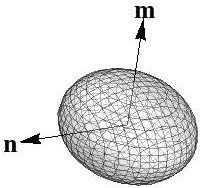
Figure 1: Sketch of an ellipsoidal Brownian particle. The two vectors $\boldsymbol{n}$ and $\boldsymbol{m}$ are attached to the particle to parametrize its rotational position, see also main text, in particular Eqs. (2b).

The equations of motion (1), (2) generate, for given initial position and orientation of the ellipsoid, stochastic trajectories in translational and orientational configuration space. According to stochastic thermodynamics jarzynski11 ; seifert12 , an entropy production $\Delta S$ is associated with such stochastic trajectories, which involves contributions from the change of particle entropy $\Delta S_{\mathrm{p}}$ and from the entropy production in the environment $\Delta S_{\mathrm{env}}$,

$$\Delta S=\Delta S_{\mathrm{p}}+\Delta S_{\mathrm{env}}\,.$$ (4)

We briefly summarize the well-known results for translational Brownian motion seifert05 and extend them to include rotational stochastic dynamics.

The particle entropy is defined as the state function seifert05

$$S_{\mathrm{p}}=-k_{\mathrm{B}}\,\ln p(\boldsymbol{x},\boldsymbol{v},\boldsymbol{n},\boldsymbol{m},\boldsymbol{\omega},t)\,,$$ (5)

where $p(\boldsymbol{x},\boldsymbol{v},\boldsymbol{n},\boldsymbol{m},\boldsymbol{\omega},t)$ is the solution of the Fokker-Planck equation associated with (1), (2). In our case, $S_{\mathrm{p}}$ does not only depend on translational degrees of freedom but also includes particle orientation, parametrized by $\boldsymbol{n}$, $\boldsymbol{m}$ and $\boldsymbol{\omega}$. The change of particle entropy along a trajectory which starts at a point $(\boldsymbol{x}_{0},\boldsymbol{v}_{0},\boldsymbol{n}_{0},\boldsymbol{m}_{0},\boldsymbol{\omega}_{0})$ in configuration space at time $t_{0}$ and is located at a point $(\boldsymbol{x}(t),\boldsymbol{v}(t),\boldsymbol{n}(t),\boldsymbol{m}(t),\boldsymbol{\omega}(t))$ at a later time $t$ is given by

$$\Delta S_{\mathrm{p}}=k_{\mathrm{B}}\,\ln p(\boldsymbol{x}_{0},\boldsymbol{v}_{0},\boldsymbol{n}_{0},\boldsymbol{m}_{0},\boldsymbol{\omega}_{0},t_{0})\\ -k_{\mathrm{B}}\,\ln p(\boldsymbol{x}(t),\boldsymbol{v}(t),\boldsymbol{n}(t),\boldsymbol{m}(t),\boldsymbol{\omega}(t),t)\,.$$ (6)

The entropy production in the environment $\mathrm{d}S_{\mathrm{env}}$ for an infinitesimal displacement of the particle is related to the heat $\delta Q$ released to the thermal bath during this displacement,

$$\mathrm{d}S_{\mathrm{env}}=\frac{\delta Q}{T}\,.$$ (7)

Following Sekimoto’s stochastic energetics approach sekimoto10 , the heat is identified with the work done by the particle on the thermal environment Note (1). This work results from the forces the particle exerts on the environment during its movement as reaction forces to viscous friction and thermal fluctuations, such that

$$\delta Q = -[-\gamma\boldsymbol{v}+\sqrt{2k_{\mathrm{B}}T}\gamma^{1/2}\boldsymbol{\xi}(t)]\circ\boldsymbol{v}\,\mathrm{d}t$$ (8)

$$-[-\eta\boldsymbol{\omega}+\sqrt{2k_{\mathrm{B}}T}\eta^{1/2}\boldsymbol{\zeta}(t)]\circ\boldsymbol{\omega}\,\mathrm{d}t$$

for a total particle displacement consisting of a translational increment $\mathrm{d}\boldsymbol{x}=\boldsymbol{v}\mathrm{d}t$ and a rotational increment $\boldsymbol{\omega}\mathrm{d}t$ during the time step $\mathrm{d}t$. The symbol $\circ$ denotes the scalar product evaluated according to the Stratonovich rule (midpoint regularization) sekimoto10 . Note that the heat $\delta Q$ as well as its two additive contributions from translation and rotation are scalar quantities and thus invariant under rotation of reference frame, a property which we exploited in (8) by representing the translational part in laboratory coordinates and the rotational part in the body-fixed frame. The entropy produced by the particle in the environment along a stochastic trajectory is the integral of (7) over that path with $\delta Q$ given by (8). Using (1b) and (2a), and the identity $[\boldsymbol{\omega}\times(I\cdot\boldsymbol{\omega})]\cdot\boldsymbol{\omega}=0$ we find

$$\Delta S_{\mathrm{env}}=\int_{t_{0}}^{t}\frac{1}{T}\left[\boldsymbol{f}\cdot\boldsymbol{v}\,\mathrm{d}t^{\prime}+\boldsymbol{M}\cdot\boldsymbol{\omega}\,\mathrm{d}t^{\prime}\right.\\ \left.-m\boldsymbol{v}\circ\mathrm{d}\boldsymbol{v}(t^{\prime})-(I\boldsymbol{\omega})\circ\mathrm{d}\boldsymbol{\omega}(t^{\prime})\right]\,.$$ (9)

In Appendix A we verify that this entropy production in the environment can be interpreted as a measure of irreversibility chetrite08 ; vandenBroeck15 , by relating it to the ratio of probabilities of forward and time-reversed paths for the combined translational and rotational motion. We also verify that the total entropy production $\Delta S$, given by (4) with (6), (9), fulfills the usual fluctuation theorem seifert05 ,

$$\left\langle e^{-\Delta S/k_{\mathrm{B}}}\right\rangle=1\,,$$ (10)

when averaged over the path ensemble with fixed initial configuration, denoted by $\langle\ldots\rangle$. Its average is therefore always positive (by Jensen’s inequality)

$$\left\langle\Delta S\right\rangle\geq 0\,,$$ (11)

in accordance with the second law.

III Overdamped limit

As described in the Introduction, the typical system we want to study with our model (1), (2) is a colloidal ellipsoidal particle of micrometer-size (or nanometer-size) suspended in water with an inhomogeneous temperature distribution around room temperature. It is well known that in such systems the effects of the fluid bath in form of thermal fluctuations and viscous friction have significant influence on the particle dynamics. Indeed, viscous friction effects are by orders of magnitude larger than inertia effects purcell77 ; dusenbery11 , so that one typically disregards inertia completely and adopts the so-called overdamped approximation by simply putting mass equal to zero, $m=0$. In a strict mathematical sense, however, this is generally not a valid procedure as it changes the order of the differential equations of motion (1), (2), so that small inertia effects (as compared to friction forces) actually correspond to a singular perturbation. Therefore, the overdamped limit should be performed with some care in a genuine perturbative way. Although the overdamped approximation and the overdamped limit give identical results in many cases, this can not be taken for granted, in particular for stochastic differential equations like (1), (2) ryter81 ; sancho82 ; jayannavar95 ; hottovy12 ; yang13 ; widder89 ; freidlin04 ; lau07 , involving heterogeneous heat baths, or for functionals along stochastic trajectories generated by (1), (2), like heat celani12 ; matsuo00 or the entropy production (9) celani12 ; bo14 ; lan15 .

III.1 Multiple time-scales

A standard tool for the rigorous derivation of singular limits is the so-called multiple time-scale technique bender99 , which exploits that the singular limit is tied to the appearance of various well-separated dynamical time-scales in the system. In our case, the dominance of viscous friction over inertia effects is related to the existence of two distinct time-scales in the equations of motion (1), (2). The first one is the time over which the velocity degrees of freedom relax and reach their stationary distribution. It is given by

$$\tau_{v}=\frac{m}{\gamma_{0}}\,,$$ (12)

where $\gamma_{0}$ is the “typical” friction coefficient of the particle, e.g., for a spherical particle of radius $a$ it corresponds to Stokes friction $\gamma_{0}=6\pi\nu a$ ($\nu$ is the dynamic viscosity of the medium the particle is suspended in). For a micrometer-sized particle in water, $\tau_{v}$ is of the order of microseconds purcell77 . The second time-scale is the time after which one can observe the diffusive motion of the particle over a detectable distance, typically about the particle size $a$,

$$\tau_{x}=\frac{a^{2}\gamma_{0}}{k_{\mathrm{B}}T_{0}}\,,$$ (13)

with $T_{0}$ being the average temperature of the bath. Under identical conditions, i.e. for a micrometer-sized particle in water, $\tau_{x}$ is of the order of seconds. Note that although we have based our definitions of $\tau_{v}$ and $\tau_{x}$ on translational motion, the time-scales for rotation are basically the same, because the “rotational mass” (i.e. moment of inertia) scales as $I\sim ma^{2}$ and the rotational viscous friction as $\eta\sim\gamma a^{2}$.

Based on this separation of time-scales, we calculate the overdamped limit of the entropy production (4) [with (6), (9)] using the multiple time-scale method. It is convenient to perform this limit for the generating function of the entropy production in the environment (9) celani12 . As side results, we then find the well-known overdamped versions of the equations of motion (1), (2), as well as the relation connecting the probability density $p$ in (5) with its overdamped counterpart. The latter is needed to deduce the overdamped limit of the change in particle entropy (6), and from that the full entropy production (4).

III.2 Generating function

In order to define the generating function of the entropy production in the environment $\Delta S_{\mathrm{env}}$, we first rewrite (9) as an integral in $\mathrm{d}t^{\prime}$ only. Observing that $k_{\mathrm{B}}\,\mathrm{d}[{(I\boldsymbol{\omega})\cdot\boldsymbol{\omega}}/{2k_{\mathrm{B}}T}]=k_{\mathrm{B}}\,\mathrm{d}[{\boldsymbol{\omega}^{\mkern-1.5mu\mathsf{T}}I\boldsymbol{\omega}}/{2k_{\mathrm{B}}T}]=(I\boldsymbol{\omega})\circ\mathrm{d}\boldsymbol{\omega}/T-[{\boldsymbol{\omega}^{\mkern-1.5mu\mathsf{T}}I\boldsymbol{\omega}}/{2T^{2}}]\,\mathrm{d}T$ and that also $k_{\mathrm{B}}\,\mathrm{d}[{\boldsymbol{\omega}^{\mkern-1.5mu\mathsf{T}}I\boldsymbol{\omega}}/{2k_{\mathrm{B}}T}]=-k_{\mathrm{B}}\,\mathrm{d}\ln w_{\omega}-(3k_{\mathrm{B}}/2T)\,\mathrm{d}T$ with the Maxwell-Boltzmann distribution for the angular velocity

$$w_{\omega}=\frac{\sqrt{\det(I)}}{(2\pi k_{\mathrm{B}}T)^{3/2}}\exp\left[-\frac{\boldsymbol{\omega}^{\mkern-1.5mu\mathsf{T}}I\boldsymbol{\omega}}{2k_{\mathrm{B}}T}\right]\,,$$ (14a)

we may write $$-(I\boldsymbol{\omega})\circ\mathrm{d}\boldsymbol{\omega}/T k_{\mathrm{B}}\,\mathrm{d}\ln w_{\omega}+[(3k_{\mathrm{B}}T-{\boldsymbol{\omega}^{\mkern-1.5mu\mathsf{T}}I\boldsymbol{\omega}})/{2T^{2}}]\,\mathrm{d}T -m\boldsymbol{v}\circ\mathrm{d}\boldsymbol{v} k_{\mathrm{B}}\,\mathrm{d}\ln w_{v}+[(3k_{\mathrm{B}}T-m\boldsymbol{v}^{2})/{2T^{2}}]\,\mathrm{d}T$$ in (9) as . The term can be recast in a similar way as by making use of the Maxwell-Boltmann distribution for the translational velocity,

$$w_{v}=\left(\frac{m}{2\pi k_{\mathrm{B}}T}\right)^{3/2}\exp\left[-\frac{m\boldsymbol{v}^{2}}{2k_{\mathrm{B}}T}\right]\,.$$ (14b)

The $\mathrm{d}T$ contributions are a consequence of the inhomogeneity of the thermal environment leading to temperature variations along the particle trajectory, which are given as $\mathrm{d}T=(\partial T/\partial t+\boldsymbol{v}\cdot\partial T/\partial\boldsymbol{x})\,\mathrm{d}t$ according to (3a), where $\partial T/\partial\boldsymbol{x}=(\partial T/\partial x_{1},\partial T/\partial x_{2},\partial T/\partial x_{3})$.

Collecting all these pieces together, we rearrange the resulting stochastic integral into three parts celani12 , $\Delta S_{\mathrm{reg}}$, $\Delta S_{\mathrm{time}}$ and $\Delta S_{\mathrm{anom}}$, related to the regular entropy production, an entropy production due to time-changes of $T$, and a part of the entropy production related to spatial temperature variations, which we show to yield an anomalous contribution in the overdamped limit. The final result for $\Delta S_{\mathrm{env}}$ from (9) thus reads

$$\Delta S_{\mathrm{env}}=-k_{\mathrm{B}}\ln w_{v}(t_{0})w_{\omega}(t_{0})+k_{\mathrm{B}}\ln w_{v}(t)w_{\omega}(t)\\ +\Delta S_{\mathrm{reg}}+\Delta S_{\mathrm{time}}+\Delta S_{\mathrm{anom}}$$ (15)

with

$$\Delta S_{\mathrm{reg}} = \int_{t_{0}}^{t}\left(\frac{\boldsymbol{f}\cdot\boldsymbol{v}}{T}-\frac{\boldsymbol{v}}{T}\cdot\frac{\partial k_{\mathrm{B}}T}{\partial\boldsymbol{x}}+\frac{\boldsymbol{M}\cdot\boldsymbol{\omega}}{T}\right)\mathrm{d}t^{\prime}\,,$$ (16a)

$$\Delta S_{\mathrm{time}} = \int_{t_{0}}^{t}\left(\frac{3k_{\mathrm{B}}T-m\boldsymbol{v}^{2}}{2T^{2}}+\frac{3k_{\mathrm{B}}T-\boldsymbol{\omega}^{\mkern-1.5mu\mathsf{T}}I\boldsymbol{\omega}}{2T^{2}}\right)\frac{\partial T}{\partial t}\,\mathrm{d}t^{\prime}\,,$$ (16b)

$$\Delta S_{\mathrm{anom}} = \int_{t_{0}}^{t}\left(\frac{5k_{\mathrm{B}}T-m\boldsymbol{v}^{2}}{2T^{2}}+\frac{3k_{\mathrm{B}}T-\boldsymbol{\omega}^{\mkern-1.5mu\mathsf{T}}I\boldsymbol{\omega}}{2T^{2}}\right)\boldsymbol{v}\cdot\frac{\partial T}{\partial\boldsymbol{x}}\,\mathrm{d}t^{\prime}\,,$$ (16c)

By splitting the entropy production into these three contributions we can essentially separate the effects of time- and spatial variations of temperature, (16b) and (16c), from the usual “regular” contribution (16a). We point out though that the regular part (16a), contains a temperature-gradient term, which is compensated by the factor 5/2 (instead of 3/2) in the first term of (16c). The appearance of the temperature-gradient is inspired by the (a posteriori) observation that the entropy production in the overdamped approximation, when inertia effects are simply disregarded, exactly corresponds to the expression (16a). This can be verified by calculating path probability ratios, see chetrite08 and the Supplementary Material of celani12 .

The joint generating function of the three contributions (16) to the entropy production is celani12

$$G_{s_{1}s_{2}s_{3}}(\boldsymbol{x},\boldsymbol{v},\boldsymbol{n},\boldsymbol{m},\boldsymbol{\omega},t|\boldsymbol{x}_{0},\boldsymbol{v}_{0},\boldsymbol{n}_{0},\boldsymbol{m}_{0},\boldsymbol{\omega}_{0},t_{0})=\left\langle\exp(-s_{1}\Delta S_{\mathrm{reg}}-s_{2}\Delta S_{\mathrm{time}}-s_{3}\Delta S_{\mathrm{anom}})\right.\\ \left.\delta(\boldsymbol{x}(t)-\boldsymbol{x})\delta(\boldsymbol{v}(t)-\boldsymbol{v})\delta(\boldsymbol{n}(t)-\boldsymbol{n})\delta(\boldsymbol{m}(t)-\boldsymbol{m})\delta(\boldsymbol{\omega}(t)-\boldsymbol{\omega})\right\rangle\,,$$ (17)

where the average is taken over paths with fixed initial conditions $\boldsymbol{x}_{0}$, $\boldsymbol{v}_{0}$, $\boldsymbol{n}_{0}$, $\boldsymbol{m}_{0}$, $\boldsymbol{\omega}_{0}$ at time $t_{0}$, as before. It can be shown to obey the forward Feynman-Kac formula mazo02 ; celani12

$$\frac{\partial G_{s_{1}s_{2}s_{3}}}{\partial t}-{\cal{A}}^{\dagger}G_{s_{1}s_{2}s_{3}}=-\left[s_{1}\left(\frac{\boldsymbol{f}\cdot\boldsymbol{v}}{T}-\frac{\boldsymbol{v}}{T}\cdot\frac{\partial k_{\mathrm{B}}T}{\partial\boldsymbol{x}}+\frac{\boldsymbol{M}\cdot\boldsymbol{\omega}}{T}\right)+s_{2}\left(\frac{3k_{\mathrm{B}}T-m\boldsymbol{v}^{2}}{2T^{2}}+\frac{3k_{\mathrm{B}}T-\boldsymbol{\omega}^{\mkern-1.5mu\mathsf{T}}I\boldsymbol{\omega}}{2T^{2}}\right)\frac{\partial T}{\partial t}\right.\\ \left.+s_{3}\left(\frac{5k_{\mathrm{B}}T-m\boldsymbol{v}^{2}}{2T^{2}}+\frac{3k_{\mathrm{B}}T-\boldsymbol{\omega}^{\mkern-1.5mu\mathsf{T}}I\boldsymbol{\omega}}{2T^{2}}\right)\boldsymbol{v}\cdot\frac{\partial T}{\partial\boldsymbol{x}}\right]G_{s_{1}s_{2}s_{3}}\,.$$ (18)

Note that for $s_{1}=0$, $s_{2}=0$, and $s_{3}=0$, the generating function represents the probability density $p$ used in (5),

$$G_{000}(\boldsymbol{x},\boldsymbol{v},\boldsymbol{n},\boldsymbol{m},\boldsymbol{\omega},t|\boldsymbol{x}_{0},\boldsymbol{v}_{0},\boldsymbol{n}_{0},\boldsymbol{m}_{0},\boldsymbol{\omega}_{0},t_{0}) = \left\langle\delta(\boldsymbol{x}(t)-\boldsymbol{x})\delta(\boldsymbol{v}(t)-\boldsymbol{v})\delta(\boldsymbol{n}(t)-\boldsymbol{n})\delta(\boldsymbol{m}(t)-\boldsymbol{m})\delta(\boldsymbol{\omega}(t)-\boldsymbol{\omega})\right\rangle$$ (19)

$$= p(\boldsymbol{x},\boldsymbol{v},\boldsymbol{n},\boldsymbol{m},\boldsymbol{\omega},t)\,.$$

Accordingly, the operator ${\cal{A}}^{\dagger}$ is the generator of the combined diffusion process for translation and rotation associated with (1), (2); its specific expression is given below in Eq. (24) (in dimensionless form).

III.3 Dimensionless representation

Since inertial effects in (1), (2) are orders of magnitude smaller than friction and other forces, the various terms in (18) may be of considerably different magnitude as well. For a detailed analysis, we rewrite all quantities appearing in (18) by introducing dimensionless representations of order one, so that the different magnitudes of terms show up as dimensionless small (or large) prefactors, which we expect to be related to the ratio of the two distinct time-scales $\tau_{v}$ and $\tau_{x}$ (see (12) and (13)). Our choice is guided by physical intuition and by the characteristics of the systems we intend to model with (1), (2). Most importantly, due to the separation of time-scales $\tau_{v}\ll\tau_{x}$, we expect the (translational and rotational) velocity degrees of freedom to equilibrate “instantaneously” and become of the order the thermal velocity. In contrast, positional degrees of freedom change significantly only on the “large” scales $a$ and $\tau_{x}$, so that we measure length and time using these units. External forces and torques are assumed to be of about the same size as the thermal fluctuating forces. We therefore make the following ansatz for relating dimensionfull and dimensionless quantities (denoted by a tilde):

$$t =\tau_{x}\tilde{t}\,,$$ (20a)

$$\boldsymbol{v} =\sqrt{\frac{k_{\mathrm{B}}T_{0}}{m}}\tilde{\boldsymbol{v}}\,, \boldsymbol{\omega} =\sqrt{\frac{k_{\mathrm{B}}T_{0}}{ma^{2}}}\tilde{\boldsymbol{\omega}}\,,$$ (20b)

$$\boldsymbol{x} =a\tilde{\boldsymbol{x}}\,, \boldsymbol{n} =\tilde{\boldsymbol{n}}\,,\;\boldsymbol{m}=\tilde{\boldsymbol{m}},$$ (20c)

$$\boldsymbol{f} =\frac{k_{\mathrm{B}}T_{0}}{a}\tilde{\boldsymbol{f}}\,, \boldsymbol{M} =k_{\mathrm{B}}T_{0}\tilde{\boldsymbol{M}}\,.$$ (20d)

We furthermore express $$I m a$$ in terms of and the length-scale ,

$$I=ma^{2}\tilde{I}\,,$$ (20e)

the friction tensors in terms of the “typical” friction coefficient $$\gamma_{0}$$,

$$\gamma=\gamma_{0}\tilde{\gamma}\,,\quad\eta=\gamma_{0}a^{2}\tilde{\eta}\,,$$ (20f)

and the temperature field by the average temperature $$T_{0}$$,

$$k_{\mathrm{B}}T=k_{\mathrm{B}}T_{0}\,\tilde{T}\,.$$ (20g)

Plugging the relations (20) into (18) and defining the dimensionless variable $\tilde{s_{i}}=k_{\mathrm{B}}s_{i}$, we obtain the dimensionless form of the forward Feynman-Kac equation

$$\left(\frac{\partial}{\partial\tilde{t}}-\varepsilon^{-1}\tilde{{\cal{L}}}^{\dagger}-\varepsilon^{-2}\tilde{{\cal{M}}}^{\dagger}-\tilde{{\cal{N}}}^{\dagger}\right)G_{\tilde{s}_{1}\tilde{s}_{2}\tilde{s}_{3}}=0\,,$$ (21)

with

$$\tilde{{\cal{L}}}^{\dagger} =-\tilde{v}_{i}\frac{\partial}{\partial\tilde{x}_{i}}-\tilde{f}_{i}\frac{\partial}{\partial\tilde{v}_{i}}-\epsilon_{ijk}\tilde{\omega}_{j}\left(\frac{\partial}{\partial\tilde{n}_{i}}\tilde{n}_{k}+\frac{\partial}{\partial\tilde{m}_{i}}\tilde{m}_{k}\right)-(\tilde{I}^{-1})_{ij}\tilde{M}_{j}\frac{\partial}{\partial\tilde{\omega}_{i}}+(\tilde{I}^{-1})_{ij}\tilde{I}_{lm}\epsilon_{jkl}\frac{\partial}{\partial\tilde{\omega}_{i}}\tilde{\omega}_{k}\tilde{\omega}_{m}$$

$$\qquad-\tilde{s}_{1}\left[\frac{\tilde{f}_{i}\tilde{v}_{i}}{\tilde{T}}-\frac{\tilde{v}_{i}}{\tilde{T}}\left(\frac{\partial\tilde{T}}{\partial\tilde{x}_{i}}\right)+\frac{\tilde{M}_{i}\tilde{\omega}_{i}}{\tilde{T}}\right]-\tilde{s}_{3}\left(\frac{5\tilde{T}\tilde{v}_{i}-\tilde{v}_{j}\tilde{v}_{j}\tilde{v}_{i}}{2\tilde{T}^{2}}+\frac{3\tilde{T}\tilde{v}_{i}-\tilde{I}_{jk}\tilde{\omega}_{j}\tilde{\omega}_{k}\tilde{v}_{i}}{2\tilde{T}^{2}}\right)\left(\frac{\partial\tilde{T}}{\partial\tilde{x}_{i}}\right)\,,$$ (22a)

$$\tilde{{\cal{M}}}^{\dagger} =\tilde{\gamma}_{ij}\frac{\partial}{\partial\tilde{v}_{i}}\tilde{v}_{j}+\tilde{T}\tilde{\gamma}_{ij}\frac{\partial}{\partial\tilde{v}_{i}}\frac{\partial}{\partial\tilde{v}_{j}}+(\tilde{I}^{-1})_{ij}\tilde{\eta}_{jk}\frac{\partial}{\partial\tilde{\omega}_{i}}\tilde{\omega}_{k}+\tilde{T}(\tilde{I}^{-1})_{il}(\tilde{I}^{-1})_{kj}\tilde{\eta}_{lk}\frac{\partial}{\partial\tilde{\omega}_{i}}\frac{\partial}{\partial\tilde{\omega}_{j}}\,,$$ (22b)

$$\tilde{{\cal{N}}}^{\dagger} =-\tilde{s}_{2}\left(\frac{3\tilde{T}-\tilde{v}_{i}\tilde{v}_{i}}{2\tilde{T}^{2}}+\frac{3\tilde{T}-\tilde{I}_{ij}\tilde{\omega}_{i}\tilde{\omega}_{j}}{2\tilde{T}^{2}}\right)\left(\frac{\partial\tilde{T}}{\partial\tilde{t}}\right)\,,$$ (22c)

where we switched to index notation for convenience with summation over repeated indices being understood. In (21), we defined

$$\varepsilon=\sqrt{\frac{\tau_{v}}{\tau_{x}}}\ll 1$$ (23)

as small parameter, expressing the time-scale separation in the system. Note that the dimensionless version $\tilde{{\cal{A}}}^{\dagger}$ of the generator ${\cal{A}}^{\dagger}$ of the diffusion process used in (18) is given as

$$\tilde{{\cal{A}}}^{\dagger} = \left[\varepsilon^{-1}\tilde{{\cal{L}}}^{\dagger}+\varepsilon^{-2}\tilde{{\cal{M}}}^{\dagger}+\tilde{{\cal{N}}}^{\dagger}\right]_{\tilde{s}_{1}=0,\tilde{s}_{2}=0,\tilde{s}_{3}=0}$$ (24)

$$= \left.\varepsilon^{-1}\tilde{{\cal{L}}}^{\dagger}\right|_{\tilde{s}_{1}=0,\tilde{s}_{3}=0}+\varepsilon^{-2}\tilde{{\cal{M}}}^{\dagger}\,.$$

III.4 Perturbation expansion

The dimensionless equation of motion (21) for the generating function (17) constitutes the starting point of our analysis, with the goal to derive its overdamped counterpart in the (singular) limit $\varepsilon=\sqrt{\tau_{v}/\tau_{x}}\to 0$. To explicitly account for the observation that the system exhibits dynamics on different time-scales we apply the following multi-scale procedure. First, we introduce time variables $\theta$ and $\tau$ corresponding to the scales given by $\tau_{v}$ and $\tau_{x}$ (see (12) and (13)), and a variable $\vartheta$ for the intermediate scale celani12 ; bo14 ; pavliotis08 ,

$$\theta=\varepsilon^{-2}\tilde{t}\,,\quad\vartheta=\varepsilon^{-1}\tilde{t}\,,\quad\tau=\tilde{t}\,.$$ (25)

We assume that the external time-changes of temperature, friction coefficients, forces and torques occur on the slow time-scale $\tau$ only, so that the dimensionless versions of (3) read

$$\tilde{T} = \tilde{T}(\tilde{\boldsymbol{x}},\tau)\,,$$ (26a)

$$\tilde{\gamma} = \tilde{\gamma}(\tilde{\boldsymbol{x}},\tilde{\boldsymbol{n}},\tilde{\boldsymbol{m}},\tau)\,,$$ (26b)

$$\tilde{\eta} = \tilde{\eta}(\tilde{\boldsymbol{x}},\tau)\,,$$ (26c)

$$\tilde{\boldsymbol{f}} = \tilde{\boldsymbol{f}}(\tilde{\boldsymbol{x}},\tilde{\boldsymbol{n}},\tilde{\boldsymbol{m}},\tau)\,,$$ (26d)

$$\tilde{\boldsymbol{M}} = \tilde{\boldsymbol{M}}(\tilde{\boldsymbol{x}},\tilde{\boldsymbol{n}},\tilde{\boldsymbol{m}},\tau)\,.$$ (26e)

Then, we expand $G_{\tilde{s}_{1}\tilde{s}_{2}\tilde{s}_{3}}$ in powers of $\varepsilon$,

$$G_{\tilde{s}_{1}\tilde{s}_{2}\tilde{s}_{3}}=G^{(0)}+\varepsilon G^{(1)}+\varepsilon^{2}G^{(2)}+\ldots\,,$$ (27)

where all the $G^{(i)}$ are a priori assumed to be functions of all variables $\tilde{\boldsymbol{x}}$, $\tilde{\boldsymbol{v}}$, $\tilde{\boldsymbol{n}}$, $\tilde{\boldsymbol{m}}$, $\tilde{\boldsymbol{\omega}}$ and of all the three different times $\theta$, $\vartheta$, $\tau$ defined in (25) (of course they also depend on the parameters $\tilde{s}_{1}$, $\tilde{s}_{2}$, $\tilde{s}_{3}$, but we skip the corresponding subscripts for notational simplicity). As a consequence, the time-derivative in (21) turns into

$$\frac{\partial}{\partial\tilde{t}}=\varepsilon^{-2}\frac{\partial}{\partial\theta}+\varepsilon^{-1}\frac{\partial}{\partial\vartheta}+\frac{\partial}{\partial\tau}\,.$$ (28)

Inserting (27), (28) into (21) and equating terms of equal power in $\varepsilon$, we find a hierarchy of coupled equations with lowest order (order $\varepsilon^{-2}$)

$$\frac{\partial G^{(0)}}{\partial\theta}-\tilde{{\cal{M}}}^{\dagger}G^{(0)}=0\,.$$ (29)

From (22b) we see that $\tilde{{\cal{M}}}^{\dagger}$ is an operator in the fast degrees of freedom $\boldsymbol{v}$, $\boldsymbol{\omega}$ only, so that their dynamics is indeed tied to the fast time $\theta$, as expected. Since there are no explicit $\theta$ dependences in $\tilde{{\cal{M}}}^{\dagger}$ (see (26)), and since we are not interested in the relaxation processes of the fast degrees of freedom on $\theta$ time-scales, we can set $\partial G^{(i)}/\partial\theta=0$ (for all $i$) in the following. Then, the first three in the hierarchy of equations read

$$\tilde{{\cal{M}}}^{\dagger}G^{(0)} =0\,,$$ (30a)

$$\tilde{{\cal{M}}}^{\dagger}G^{(1)} =\frac{\partial G^{(0)}}{\partial\vartheta}-\tilde{{\cal{L}}}^{\dagger}G^{(0)}\,,$$ (30b)

$$\tilde{{\cal{M}}}^{\dagger}G^{(2)} =\frac{\partial G^{(0)}}{\partial\tau}-\tilde{{\cal{N}}}^{\dagger}G^{(0)}+\frac{\partial G^{(1)}}{\partial\vartheta}-\tilde{{\cal{L}}}^{\dagger}G^{(1)}\,,$$ (30c)

with the first line collecting order $\varepsilon^{-2}$ terms, the second line order $\varepsilon^{-1}$ terms and the third line order $\varepsilon^{0}$ terms.

The solution to (30a) is

$$G^{(0)}=g^{(0)}(\tilde{\boldsymbol{x}},\tilde{\boldsymbol{n}},\tilde{\boldsymbol{m}},\vartheta,\tau)\tilde{w}_{v}(\tilde{\boldsymbol{v}}|\tilde{\boldsymbol{x}},\tau)\tilde{w}_{\omega}(\tilde{\boldsymbol{\omega}}|\tilde{\boldsymbol{x}},\tau)\,,$$ (31)

where $\tilde{w}_{v}(\tilde{\boldsymbol{v}}|\tilde{\boldsymbol{x}},\tau)$ and $\tilde{w}_{\omega}(\tilde{\boldsymbol{\omega}}|\tilde{\boldsymbol{x}},\tau)$ are the dimensionless counterparts of the Maxwell-Boltzmann distributions for translational and rotational velocity (at given position and time) defined in (14) Note (2), and where $g^{(0)}(\tilde{\boldsymbol{x}},\tilde{\boldsymbol{n}},\tilde{\boldsymbol{m}},\vartheta,\tau)$ is an unknown function of only the slow degrees of freedom according to the general definition

$$g^{(i)}(\tilde{\boldsymbol{x}},\tilde{\boldsymbol{n}},\tilde{\boldsymbol{m}},\vartheta,\tau)=\int\mathrm{d}\tilde{\boldsymbol{v}}\mathrm{d}\tilde{\boldsymbol{\omega}}\,G^{(i)}\,.$$ (32)

To proceed with the higher order equations (30b), (30c) we employ the solvability condition. It states that the inhomogeneities on the right-hand sides need to be orthogonal to the nullspace of the operator $\tilde{{\cal{M}}}$ adjoint to $\tilde{{\cal{M}}}^{\dagger}$ (Fredholm alternative, see, e.g., pavliotis08 ). As we can see from (22b), the nullspace of $\tilde{{\cal{M}}}$ contains the functions which are constant in $\tilde{\boldsymbol{v}}$ and $\tilde{\boldsymbol{\omega}}$. Therefore, the solvability condition for (30b) reads $\int\mathrm{d}\tilde{\boldsymbol{v}}\mathrm{d}\tilde{\boldsymbol{\omega}}\,(\partial G^{(0)}/\partial\vartheta-\tilde{{\cal{L}}}^{\dagger}G^{(0)})=0$. It is straightforward to show from the explicit expression (22a) for $\tilde{{\cal{L}}}^{\dagger}$ that $\int\mathrm{d}\tilde{\boldsymbol{v}}\mathrm{d}\tilde{\boldsymbol{\omega}}\,\tilde{{\cal{L}}}^{\dagger}G^{(0)}=0$, so that we find $g^{(0)}$ in (31) to be independent of the intermediate time-scale $\vartheta$,

$$\frac{\partial g^{(0)}}{\partial\vartheta}=0\,.$$ (33)

Applying the solvability condition in an analogous way to (30c) we obtain

$$\frac{\partial g^{(0)}}{\partial\tau}+\frac{\partial g^{(1)}}{\partial\vartheta}=\int\mathrm{d}\tilde{\boldsymbol{v}}\mathrm{d}\tilde{\boldsymbol{\omega}}\,\tilde{{\cal{L}}}^{\dagger}G^{(1)}\,,$$ (34)

where we have used $\int\mathrm{d}\tilde{\boldsymbol{v}}\mathrm{d}\tilde{\boldsymbol{\omega}}\,\tilde{{\cal{N}}}^{\dagger}G^{(0)}=0$.

We can now state more precisely what it means to derive the overdamped equation of motion for the generating function $G_{\tilde{s}_{1}\tilde{s}_{2}\tilde{s}_{3}}$. This overdamped equation should be valid only on time-scales beyond those of $\theta$, after the fast degrees of freedom have relaxed and have reached their stationary distribution (on $\theta$ time-scales), so that they can be integrated out. The overdamped generating function is thus given by

$$g_{\tilde{s}_{1}\tilde{s}_{2}\tilde{s}_{3}}=\lim_{\varepsilon\to 0}\int\mathrm{d}\tilde{\boldsymbol{v}}\mathrm{d}\tilde{\boldsymbol{\omega}}\,G_{\tilde{s}_{1}\tilde{s}_{2}\tilde{s}_{3}}\,,$$ (35)

for which we want to calculate the equation of motion

$$\frac{\partial g_{\tilde{s}_{1}\tilde{s}_{2}\tilde{s}_{3}}}{\partial\tilde{t}}=\lim_{\varepsilon\to 0}\int\mathrm{d}\tilde{\boldsymbol{v}}\mathrm{d}\tilde{\boldsymbol{\omega}}\,\frac{\partial G_{\tilde{s}_{1}\tilde{s}_{2}\tilde{s}_{3}}}{\partial\tilde{t}}\,.$$ (36)

The overdamped limit $\varepsilon=\sqrt{\tau_{v}/\tau_{x}}\to 0$ singles out the zeroth-order contribution in $G_{\tilde{s}_{1}\tilde{s}_{2}\tilde{s}_{3}}$ and ${\partial G_{\tilde{s}_{1}\tilde{s}_{2}\tilde{s}_{3}}}/{\partial\tilde{t}}$. It follows from (27), (31) that $g_{\tilde{s}_{1}\tilde{s}_{2}\tilde{s}_{3}}$ is actually identical to $g^{(0)}$. Moreover, inserting the relations (27) and (28) into (36), and using the results we so far obtained from the perturbation expansion, namely $\partial G^{(0)}/\partial\theta=0$, as well as (33) and (34), we find

$$\frac{\partial g_{\tilde{s}_{1}\tilde{s}_{2}\tilde{s}_{3}}}{\partial\tilde{t}}=\int\mathrm{d}\tilde{\boldsymbol{v}}\mathrm{d}\tilde{\boldsymbol{\omega}}\,\tilde{{\cal{L}}}^{\dagger}G^{(1)}\,.$$ (37)

In the integral on the right-hand side the $\partial/\partial\tilde{v}_{i}$ and $\partial/\partial\tilde{\omega}_{i}$ terms from (22a) evaluate to zero. Our quantity of interest therefore becomes

$$\frac{\partial g_{\tilde{s}_{1}\tilde{s}_{2}\tilde{s}_{3}}}{\partial\tilde{t}}=-\frac{\partial J_{\tilde{v}_{i}}}{\partial\tilde{x}_{i}}-\epsilon_{ijk}\left(\frac{\partial}{\partial\tilde{n}_{i}}\tilde{n}_{k}+\frac{\partial}{\partial\tilde{m}_{i}}\tilde{m}_{k}\right)J_{\tilde{\omega}_{j}}\\ -\tilde{s}_{1}\left[\frac{\tilde{f}_{i}J_{\tilde{v}_{i}}}{\tilde{T}}-\frac{J_{\tilde{v}_{i}}}{\tilde{T}}\frac{\partial\tilde{T}}{\partial\tilde{x}_{i}}+\frac{\tilde{M}_{i}J_{\tilde{\omega}_{i}}}{\tilde{T}}\right]\\ -\tilde{s}_{3}\left(\frac{5\tilde{T}J_{\tilde{v}_{i}}-J_{\tilde{v}_{j}\tilde{v}_{j}\tilde{v}_{i}}}{2\tilde{T}^{2}}+\frac{3\tilde{T}J_{\tilde{v}_{i}}-J_{\tilde{I}_{jk}\tilde{\omega}_{j}\tilde{\omega}_{k}\tilde{v}_{i}}}{2\tilde{T}^{2}}\right)\frac{\partial\tilde{T}}{\partial\tilde{x}_{i}}\,,$$ (38)

with the definition

$$J_{\pi(\tilde{\boldsymbol{v}},\tilde{\boldsymbol{\omega}})}=\int\mathrm{d}\tilde{\boldsymbol{v}}\mathrm{d}\tilde{\boldsymbol{\omega}}\,\pi(\tilde{\boldsymbol{v}},\tilde{\boldsymbol{\omega}})G^{(1)}$$ (39)

for integrals over (polynomial) functions $\pi(\tilde{\boldsymbol{v}},\tilde{\boldsymbol{\omega}})$ in $\tilde{\boldsymbol{v}}$ and $\tilde{\boldsymbol{\omega}}$ multiplying $G^{(1)}$. We remark that (38) does not depend explicitly on $\tilde{s}_{2}$, as $G^{(1)}$ is independent of $\tilde{s}_{2}$ according to (30b), with the consequence that in the overdamped limit the temperature variations with time do not show up directly. For evaluating the remaining various integrals $J_{\pi(\tilde{\boldsymbol{v}},\tilde{\boldsymbol{\omega}})}$ appearing in (38), it is actually not necessary to find the full solution $G^{(1)}$ of (30b). Instead, they can be evaluated directly from (30b) using the known solution (31) for $G^{(0)}$, as shown in Appendix B. The final result reads

$$\frac{\partial g_{\tilde{s}_{1}\tilde{s}_{2}\tilde{s}_{3}}}{\partial\tilde{t}}=-\frac{\partial}{\partial\tilde{x}_{i}}\left[(\tilde{\gamma}^{-1})_{ij}\tilde{f}_{j}-(\tilde{\gamma}^{-1})_{ij}\frac{\partial}{\partial\tilde{x}_{j}}\tilde{T}\right]g_{\tilde{s}_{1}\tilde{s}_{2}\tilde{s}_{3}}\\ -\epsilon_{ijk}\left(\frac{\partial}{\partial\tilde{n}_{i}}\tilde{n}_{k}+\frac{\partial}{\partial\tilde{m}_{i}}\tilde{m}_{k}\right)\left[(\tilde{\eta}^{-1})_{jl}\tilde{M}_{l}-(\tilde{\eta}^{-1})_{jl}\tilde{T}\epsilon_{plq}\left(\frac{\partial}{\partial\tilde{n}_{p}}\tilde{n}_{q}+\frac{\partial}{\partial\tilde{m}_{p}}\tilde{m}_{q}\right)\right]g_{\tilde{s}_{1}\tilde{s}_{2}\tilde{s}_{3}}\\ -\tilde{s}_{1}\left[\tilde{T}(\tilde{\gamma}^{-1})_{ij}\frac{\partial}{\partial\tilde{x}_{j}}\left(\frac{\tilde{f}_{i}}{\tilde{T}}-\frac{1}{\tilde{T}}\frac{\partial\tilde{T}}{\partial\tilde{x}_{i}}\right)+\left((\tilde{\gamma}^{-1})_{ij}\tilde{f}_{j}+\tilde{T}\frac{\partial(\tilde{\gamma}^{-1})_{ij}}{\partial\tilde{x}_{j}}\right)\left(\frac{\tilde{f}_{i}}{\tilde{T}}-\frac{1}{\tilde{T}}\frac{\partial\tilde{T}}{\partial\tilde{x}_{i}}\right)\right]g_{\tilde{s}_{1}\tilde{s}_{2}\tilde{s}_{3}}\\ +\tilde{s}_{1}^{2}\,\tilde{T}(\tilde{\gamma}^{-1})_{ij}\left(\frac{\tilde{f}_{i}}{\tilde{T}}-\frac{1}{\tilde{T}}\frac{\partial\tilde{T}}{\partial\tilde{x}_{i}}\right)\left(\frac{\tilde{f}_{j}}{\tilde{T}}-\frac{1}{\tilde{T}}\frac{\partial\tilde{T}}{\partial\tilde{x}_{j}}\right)g_{\tilde{s}_{1}\tilde{s}_{2}\tilde{s}_{3}}+2\tilde{s}_{1}\left[\frac{\partial}{\partial\tilde{x}_{i}}(\tilde{\gamma}^{-1})_{ij}\left(\tilde{f}_{j}-\frac{\partial\tilde{T}}{\partial\tilde{x}_{j}}\right)g_{\tilde{s}_{1}\tilde{s}_{2}\tilde{s}_{3}}\right]\\ -\tilde{s}_{1}\left[\frac{(\tilde{\eta}^{-1})_{ij}}{\tilde{T}}\tilde{M}_{i}\tilde{M}_{j}+\epsilon_{ijk}(\tilde{\eta}^{-1})_{jl}\left(\tilde{n}_{k}\frac{\partial\tilde{M}_{l}}{\partial\tilde{n}_{i}}+\tilde{m}_{k}\frac{\partial\tilde{M}_{l}}{\partial\tilde{m}_{i}}\right)\right]g_{\tilde{s}_{1}\tilde{s}_{2}\tilde{s}_{3}}\\ +\tilde{s}_{1}^{2}\,\frac{(\tilde{\eta}^{-1})_{ij}}{\tilde{T}}\tilde{M}_{i}\tilde{M}_{j}g_{\tilde{s}_{1}\tilde{s}_{2}\tilde{s}_{3}}+2\tilde{s}_{1}\left[\left(\frac{\partial}{\partial\tilde{n}_{i}}\tilde{n}_{k}+\frac{\partial}{\partial\tilde{m}_{i}}\tilde{m}_{k}\right)\epsilon_{ijk}(\tilde{\eta}^{-1})_{jl}\tilde{M}_{l}g_{\tilde{s}_{1}\tilde{s}_{2}\tilde{s}_{3}}\right]\\ +\tilde{s}_{3}(\tilde{s}_{3}-1)\frac{1}{2\tilde{T}}\left(\frac{2U_{ik}U_{jk}}{3\tilde{\gamma}^{(k)}}+\sum_{l}\frac{U_{ik}U_{jk}}{\tilde{\gamma}^{(k)}+2\tilde{\gamma}^{(l)}}+\sum_{l}\frac{U_{ik}U_{jk}}{\tilde{\gamma}^{(k)}+2\tilde{\eta}^{(l)}/\tilde{I}^{(l)}}\right)\frac{\partial\tilde{T}}{\partial\tilde{x}_{i}}\frac{\partial\tilde{T}}{\partial\tilde{x}_{j}}g_{\tilde{s}_{1}\tilde{s}_{2}\tilde{s}_{3}}\,,$$ (40)

where we have used on the right-hand side that $g^{(0)}=g_{\tilde{s}_{1}\tilde{s}_{2}\tilde{s}_{3}}$, and where $U_{ik}$ is defined in Eq. (84) of Appendix B. This expression, together with its interpretation in the following Sections constitute the main results of this paper.

IV Overdamped dynamics

In analogy to (19) we obtain the overdamped limit of the probability density $\rho(\boldsymbol{x},\boldsymbol{n},\boldsymbol{m},t)=\lim_{\varepsilon\to 0}\int\mathrm{d}\boldsymbol{v}\mathrm{d}\boldsymbol{\omega}\,p(\boldsymbol{x},\boldsymbol{v},\boldsymbol{n},\boldsymbol{m},\boldsymbol{\omega},t)$ from $g_{000}$. According to (35) and (36), we can thus read off the overdamped equation of motion for $\rho(\boldsymbol{x},\boldsymbol{n},\boldsymbol{m},t)$ from (40) by setting $\tilde{s}_{1}=0$, $\tilde{s}_{2}=0$, $\tilde{s}_{3}=0$:

$$\frac{\partial\rho}{\partial t}-{\cal{A}}_{\mathrm{over}}^{\dagger}\rho=0\,,$$ (41)

with

$${\cal{A}}_{\mathrm{over}}^{\dagger}=-\frac{\partial}{\partial x_{i}}\left[(\gamma^{-1})_{ij}f_{j}-(\gamma^{-1})_{ij}\frac{\partial}{\partial x_{j}}k_{\mathrm{B}}T\right]\\ -\epsilon_{ijk}\left(\frac{\partial}{\partial n_{i}}n_{k}+\frac{\partial}{\partial m_{i}}m_{k}\right)\left[(\eta^{-1})_{jl}M_{l}-(\eta^{-1})_{jl}k_{\mathrm{B}}T\epsilon_{plq}\left(\frac{\partial}{\partial n_{p}}n_{q}+\frac{\partial}{\partial m_{p}}m_{q}\right)\right]\,,$$ (42)

where we switched back to dimensionful quantities. Here and in the following, we use a sub- or superscript “over” to indicate the overdamped limit and to differentiate overdamped quantities from the original ones. The Langevin equations, which are equivalent to the Fokker-Planck equation (41), (42), read

$$\dot{\boldsymbol{x}} = \gamma^{-1}\boldsymbol{f}-\frac{\gamma^{-1}}{2}\frac{\partial k_{\mathrm{B}}T}{\partial\boldsymbol{x}}+\frac{k_{\mathrm{B}}T}{2}\frac{\partial\gamma^{-1}}{\partial\boldsymbol{x}}$$ (43a)

$$\qquad\mbox{}+\sqrt{2k_{\mathrm{B}}T}\gamma^{-1/2}\circ\boldsymbol{\xi}(t)\,,$$

$$\dot{\boldsymbol{n}} = \left[\eta^{-1}\boldsymbol{M}+\sqrt{2k_{\mathrm{B}}T}\eta^{-1/2}\boldsymbol{\zeta}(t)\right]\times\boldsymbol{n}\,,$$ (43b)

$$\dot{\boldsymbol{m}} = \left[\eta^{-1}\boldsymbol{M}+\sqrt{2k_{\mathrm{B}}T}\eta^{-1/2}\boldsymbol{\zeta}(t)\right]\times\boldsymbol{m}\,,$$ (43c)

where $\boldsymbol{\xi}(t)$ and $\boldsymbol{\zeta}(t)$ are Gaussian white noise sources (like in (1), (2), but not related to those), and where all the products involving noise terms, even the cross products, are to be interpreted in the Stratonovich sense. These Langevin equations are well-known as a model for the overdamped translation and rotation of ellipsoidal particles mazo02 . In particular the “splitting” of the translational diffusion tensor $D=k_{\mathrm{B}}T\gamma^{-1}$ into $k_{\mathrm{B}}T$ and $\gamma^{-1}$ between the two spatial derivatives in the diffusion term of (42) has been obtained before, as well as the specific “spurious drift terms” in (43a) resulting from that “splitting” ryter81 ; sancho82 ; jayannavar95 ; hottovy12 ; yang13 . Note that the explicit form of these “spurious drift terms” and the corresponding interpretation of the noise products are a natural outcome of the systematic perturbation analysis. They can not be obtained from the overdamped approximation, naively disregarding inertia effects in (1), (2). The overdamped approximation yields correct equations only for homogeneous thermal environments when $T$, $\gamma$ and $\eta$ are constant.

V Overdamped entropy production and anomalous entropy

Based on the overdamped Langevin equations (43) we can follow the standard reasoning of stochastic thermodynamics and define the entropy production along stochastic trajectories as

$$\Delta S^{\mathrm{over}}=\Delta S_{\mathrm{p}}^{\mathrm{over}}+\Delta S_{\mathrm{env}}^{\mathrm{over}}\,.$$ (44)

It is composed of contributions from the entropy change of the particle $\Delta S_{\mathrm{p}}^{\mathrm{over}}$ and from the entropy change in the environment $\Delta S_{\mathrm{env}}^{\mathrm{over}}$. The entropy change of the particle is given as seifert05

$$\Delta S_{\mathrm{p}}^{\mathrm{over}}=k_{\mathrm{B}}\,\ln\rho(\boldsymbol{x}_{0},\boldsymbol{n}_{0},\boldsymbol{m}_{0},t_{0})\\ -k_{\mathrm{B}}\,\ln\rho(\boldsymbol{x}(t),\boldsymbol{n}(t),\boldsymbol{m}(t),t)\,,$$ (45)

for a trajectory which starts at at a point $(\boldsymbol{x}_{0},\boldsymbol{n}_{0},\boldsymbol{m}_{0})$ at time $t_{0}$ and is located at a point $(\boldsymbol{x}(t),\boldsymbol{n}(t),\boldsymbol{m}(t))$ at a later time $t$. The entropy change in the environment can in principle be defined from the heat exchanged with the environment. However, due to the variations of temperature with position such an identification is subtle for the translational degrees of freedom celani12 ; matsuo00 and thus the definition of entropy production in the environment is better based on path probability ratios chetrite08 . It reads

$$\Delta S_{\mathrm{env}}^{\mathrm{over}}=\int_{t_{0}}^{t}\frac{1}{T}\left[\left(\boldsymbol{f}-\frac{\partial k_{\mathrm{B}}T}{\partial\boldsymbol{x}}\right)\circ\mathrm{d}\boldsymbol{x}(t^{\prime})\right.\\ +(\eta^{-1}\boldsymbol{M})\cdot\boldsymbol{M}\,\mathrm{d}t^{\prime}+\sqrt{2k_{\mathrm{B}}T}\boldsymbol{M}\eta^{-1/2}\circ\mathrm{d}\boldsymbol{W}(t^{\prime})\bigg{]}\,,$$ (46)

where $\mathrm{d}\boldsymbol{W}$ is the increment of the Wiener process corresponding to the Gaussian white noise $\boldsymbol{\zeta}(t)$ in (43b), (43c). In that way, one arrives at an entropy production which is expressed as a sequential functional on overdamped trajectories.

We now compare the expressions (45) and (46), obtained from applying stochastic thermodynamics principles “naively” to the overdamped equations of motion (43), with the full result (40) from the systematic perturbation analysis. We first observe that the overdamped limit $\varepsilon\to 0$ of the probability density $p$ appearing in the change of particle entropy (6) is given by $G^{(0)}$ evaluated at $\tilde{s}_{1}=0$, $\tilde{s}_{2}=0$, $\tilde{s}_{3}=0$, which we obtain from (31) to be $\rho(\boldsymbol{x},\boldsymbol{n},\boldsymbol{m},t)w_{v}(\boldsymbol{v}|\boldsymbol{x},t)w_{\omega}(\boldsymbol{\omega}|\boldsymbol{x},t)$ (dimensionful units). Therefore, $\lim_{\varepsilon\to 0}\Delta S_{\textrm{p}}$ yields the terms listed in (45), plus additional terms involving $\log w_{v}w_{\omega}$ which cancel precisely with the first line in (15). We conclude that, in the overdamped limit, the change of the particle entropy can indeed be identified with (45), while the entropy production in the environment originates from the overdamped counterparts $\Delta S_{\mathrm{reg}}^{\mathrm{over}}$, $\Delta S_{\mathrm{time}}^{\mathrm{over}}$, $\Delta S_{\mathrm{anom}}^{\mathrm{over}}$ of the entropy terms in the second line of (15). These overdamped entropy contributions are encoded in our main result (40) by the definition

$$g_{s_{1}s_{2}s_{3}}(\boldsymbol{x},\boldsymbol{n},\boldsymbol{m},t|\boldsymbol{x}_{0},\boldsymbol{n}_{0},\boldsymbol{m}_{0},t_{0})\\ =\left\langle\exp(-s_{1}\Delta S_{\mathrm{reg}}^{\mathrm{over}}-s_{2}\Delta S_{\mathrm{time}}^{\mathrm{over}}-s_{3}\Delta S_{\mathrm{anom}}^{\mathrm{over}})\right.\\ \left.\delta(\boldsymbol{x}(t)-\boldsymbol{x})\delta(\boldsymbol{n}(t)-\boldsymbol{n})\delta(\boldsymbol{m}(t)-\boldsymbol{m})\right\rangle\,,$$ (47)

analogous to (17). To access and analyze the specific form of an individual contribution we set the $s$ variables associated with the other contributions to zero and compare the remaining terms in (40) with the general formulas from Appendix C. In that way, we find the following:

The entropy production given in (46) arises precisely from the overdamped limit of the regular part (16a), represented by the $\tilde{s}_{1}$ terms in (40). There is no contribution from the entropy production (16b) due time-changes of temperature, because (40) does not explicitly depend on $\tilde{s}_{2}$ (as already pointed out earlier), such that $\Delta S_{\mathrm{time}}^{\mathrm{over}}$ is bound to vanish identically. However, the $\tilde{s}_{3}$ terms yield additional contributions to the overdamped entropy production, which are not included in (46). From their specific functional form we infer (cf. Appendix C) that these contributions can not even be expressed as a sequential functional over overdamped trajectories. Their origin is the entropy production $\Delta S_{\mathrm{anom}}$ from (16c) (see also (17)) celani12 ; bo14 .

Although it is not possible to explicitly write this “anomalous entropy production” celani12 as an integral along paths of the overdamped dynamics, we can still derive a number of interesting and useful results on its average behavior from (40), similarly to the reasoning in the Supplementary Material of celani12 . Setting $\tilde{s}_{1}=0$, $\tilde{s}_{2}=0$, $\tilde{s}_{3}=1$ (i.e. $s_{1}=0$, $s_{2}=0$, $s_{3}=1/k_{\mathrm{B}}$) we find that $g_{001}=\langle\exp(-\Delta S_{\mathrm{anom}}^{\mathrm{over}}/k_{\mathrm{B}})\delta(\boldsymbol{x}(t)-\boldsymbol{x})\delta(\boldsymbol{n}(t)-\boldsymbol{n})\delta(\boldsymbol{m}(t)-\boldsymbol{m})\rangle$ obeys the same forward equation as $g_{000}=\rho(\boldsymbol{x},\boldsymbol{n},\boldsymbol{m},t)$, so that it has the solution

$$\left\langle\exp\left(-\Delta S_{\mathrm{anom}}^{\mathrm{over}}/k_{\mathrm{B}}\right)\right.\\ \left.\delta(\boldsymbol{x}(t)-\boldsymbol{x})\delta(\boldsymbol{n}(t)-\boldsymbol{n})\delta(\boldsymbol{m}(t)-\boldsymbol{m})\right\rangle\\ =\rho(\boldsymbol{x},\boldsymbol{n},\boldsymbol{m},t)\,.$$ (48)

Integrating over the spatial coordinates $\boldsymbol{x}$, $\boldsymbol{n}$, $\boldsymbol{m}$, we find the fluctuation relation

$$\left\langle\exp\left(-\Delta S_{\mathrm{anom}}^{\mathrm{over}}/k_{\mathrm{B}}\right)\right\rangle=1\,.$$ (49)

It follows immediately (by Jensen’s inequality) that

$$\left\langle\Delta S_{\mathrm{anom}}^{\mathrm{over}}\right\rangle\geq 0\,.$$ (50)

The explicit form for the average rate of anomalous entropy production can be obtained from (40) by observing that $\frac{\mathrm{d}}{\mathrm{d}t}\langle\Delta S_{\mathrm{anom}}^{\mathrm{over}}\rangle=-\frac{\mathrm{d}}{\mathrm{d}t}\int\mathrm{d}\boldsymbol{x}\,\mathrm{d}(\boldsymbol{n},\boldsymbol{m})\left.\partial g_{00s_{3}}/\partial s_{3}\right|_{s_{3}=0}$ (see also the derivation of Eq. (99) in Appendix C). It reads (in dimensionful quantities)

$$\frac{\mathrm{d}}{\mathrm{d}t}\langle\Delta S_{\mathrm{anom}}^{\mathrm{over}}\rangle = k_{\mathrm{B}}\left\langle\frac{1}{2T}\left(\frac{2}{3\gamma^{(k)}}+\sum_{l}\frac{1}{\gamma^{(k)}+2\gamma^{(l)}}+\sum_{l}\frac{1}{\gamma^{(k)}+2\eta^{(l)}/\frac{I^{(l)}}{m}}\right)\left(U_{ik}\frac{\partial T}{\partial x_{i}}\right)\left(U_{jk}\frac{\partial T}{\partial x_{j}}\right)\right\rangle$$ (51a)

$$= k_{\mathrm{B}}\left\langle\frac{1}{2T}\left[\frac{2}{3}\left(\gamma^{-1}\right)_{ij}+\sum_{l}\left(\left[\gamma+2\gamma^{(l)}\mathbb{I}\right]^{-1}\right)_{ij}+\sum_{l}\left(\left[\gamma+\frac{2\eta^{(l)}}{I^{(l)}/m}\mathbb{I}\right]^{-1}\right)_{ij}\right]\frac{\partial T}{\partial x_{i}}\frac{\partial T}{\partial x_{j}}\right\rangle$$ (51b)

$$= k_{\mathrm{B}}\int\mathrm{d}\boldsymbol{x}\,\mathrm{d}(\boldsymbol{n},\boldsymbol{m})\,\frac{\rho}{2T}\left(\frac{\partial T}{\partial\boldsymbol{x}}\right)^{\mkern-1.5mu\mathsf{T}}\left[\frac{2}{3}\gamma^{-1}+\sum_{l}\left(\gamma+2\gamma^{(l)}\mathbb{I}\right)^{-1}+\sum_{l}\left(\gamma+\frac{2\eta^{(l)}}{I^{(l)}/m}\mathbb{I}\right)^{-1}\right]\frac{\partial T}{\partial\boldsymbol{x}}\,.$$ (51c)

These expressions for the average rate of anomalous entropy production are another central result of the present paper. We give three different, but equivalent forms. In the first line, the entropy production is written in the coordinate frame fixed to the particle. Accordingly, the quantity $U_{ik}\frac{\partial T}{\partial x_{i}}$ is the temperature gradient along that principal axis of the particle, for which the friction coefficients are $\gamma^{(k)}$ and $\eta^{(k)}$ (and moment of inertia is $I^{(k)}$); see Eq. (84) in Appendix B where also the $U_{ik}$ are defined. The second line represents the anomalous entropy production in the laboratory frame of reference ($\mathbb{I}$ denotes the identity matrix). In the third line, we switch back to vector notation and we express the average $\langle\ldots\rangle$ over particle trajectories explicitly as an integral over the probability density $\rho=\rho(\boldsymbol{x},\boldsymbol{n},\boldsymbol{m},t)$; note that the integral over $\mathrm{d}(\boldsymbol{n},\boldsymbol{m})$ is not performed independently over $\boldsymbol{n}$ and $\boldsymbol{m}$ but rather represents an integral over the space of particle orientations, parametrized by $\boldsymbol{n}$, $\boldsymbol{m}$.

The result (51) generalizes the discovery of the anomalous entropy in celani12 in essentially two respects. First, it covers non-trivial particle shapes, quantifying deviations from a perfectly spherical bead by the principal values $\gamma^{(i)}$, $\eta^{(i)}$ and $I^{(i)}/m$. Note that the ratio $I^{(i)}/m$ does not depend on the particle mass, as $I^{(i)}$ is proportional to $m$; it is thus a purely geometrical factor reflecting the particle’s shape. Second, it takes into account the rotational degrees of freedom of the Brownian particle, and reveals that rotational motion adds to the entropy production. Partial results about the effects of rotation on the entropic anomaly have also been derived in lan15 . The rotational entropy production originates from the terms involving the rotational friction coefficients $\eta^{(i)}$, since these terms vanish when we “freeze” the particle rotation using the limit $\eta^{(i)}\to\infty$ to be left with the translational motion only. We can therefore identify the translational and rotational contributions to the anomalous entropy production as

$$\kappa_{\mathrm{trans}} = \frac{k_{\mathrm{B}}\rho}{2T}\left(\frac{2}{3}\gamma^{-1}+\sum_{l}\left(\gamma+2\gamma^{(l)}\mathbb{I}\right)^{-1}\right)\,,$$ (52a)

$$\kappa_{\mathrm{rot}} = \frac{k_{\mathrm{B}}\rho}{2T}\sum_{l}\left(\gamma+\frac{2\eta^{(l)}}{I^{(l)}/m}\mathbb{I}\right)^{-1}\,.$$ (52b)

It has been argued in celani12 that the anomalous entropy is generated by the particle permanently transporting heat between adjacent regions at different temperatures in the inhomogeneous thermal environment on the fast time-scale $\tau_{v}$ and associated length-scale $(k_{\mathrm{B}}T_{0}m)^{1/2}/\gamma_{0}$ without performing any visible displacement on the long (overdamped) time-scale $\tau_{x}$. We can therefore interpret $\kappa_{\mathrm{trans}}$ and $\kappa_{\mathrm{rot}}$ as state-dependent, anisotropic heat conductivities quantifying this process behind the anomalous entropy production lan15 . This interpretation also explains why the rotational contribution $\kappa_{\mathrm{rot}}$ depends on the translational friction coefficients $\gamma$. The conducted heat is “stored” in the rotational degrees of freedom, but is transported from one temperature region to another by translation. Without translational motion, the particle’s rotation can not produce “anomalous entropy”.

We finally remark that the rotational motion contributes to the anomalous entropy production even if the particle is perfectly spherical. For homogeneous spherical beads with radius $a$, translational and rotational friction tensors as well as the moment of inertia tensor are proportional to the unit tensor, i.e. we have happel83 $\gamma^{(1)}=\gamma^{(2)}=\gamma^{(3)}=6\pi\nu a$, $\eta^{(1)}=\eta^{(2)}=\eta^{(3)}=8\pi\nu a^{3}$ and $I^{(1)}=I^{(2)}=I^{(3)}=2ma^{2}/5$, so that the conductivities become isotropic,

$$\kappa_{\mathrm{trans}} = \frac{5k_{\mathrm{B}}\rho}{6T\gamma^{(1)}}\,\mathbb{I}=\frac{5k_{\mathrm{B}}\rho}{36\pi T\nu a}\,\mathbb{I}\,,$$ (53a)

$$\kappa_{\mathrm{rot}} = \frac{3k_{\mathrm{B}}\rho}{2T}\frac{1}{\gamma^{(1)}+2\eta^{(1)}/\frac{I^{(1)}}{m}}\,\mathbb{I}=\frac{3k_{\mathrm{B}}\rho}{92\pi T\nu a}\,\mathbb{I}\,.$$ (53b)

For the translational part we just recover the result from celani12 , while the particle rotation gives rise to an additional contribution not described in celani12 . The frictional “coefficients” $\gamma^{(1)}$ and $\eta^{(1)}/\frac{I^{(1)}}{m}$, representing translation and rotation, respectively, quantify physically related effects and are of similar magnitude. Hence, the rotational contribution to the “anomalous entropy” is well comparable to the translational part, and is actually only by about a factor four smaller (see also the discussion in lan15 ).

VI Prolate and oblate spheroids

For an ellipsoidal particle

$$\frac{x_{1}^{2}}{a_{1}^{2}}+\frac{x_{2}^{2}}{a_{2}^{2}}+\frac{x_{3}^{2}}{a_{3}^{2}}=1$$ (54)

with semi-axis lengths $a_{1}$, $a_{2}$, $a_{3}$, the translational friction coefficients $\gamma^{(i)}$ have been calculated by Oberbeck oberbeck1876 , the rotational ones $\eta^{(i)}$ by Edwardes edwardes1892 and Jeffery jeffery22 . They are summarized, for instance, in brenner67 and read

$$\gamma^{(i)} = 16\pi\nu\frac{1}{\chi+a_{i}^{2}\alpha_{i}}\quad(\mbox{for }i=1,2,3)\,,$$ (55a)

$$\eta^{(1)} = \frac{16\pi\nu}{3}\frac{a_{2}^{2}+a_{3}^{2}}{a_{2}^{2}\alpha_{2}+a_{3}^{2}\alpha_{3}}\,,$$ (55b)

$$\eta^{(2)} = \frac{16\pi\nu}{3}\frac{a_{3}^{2}+a_{1}^{2}}{a_{3}^{2}\alpha_{3}+a_{1}^{2}\alpha_{1}}\,,$$ (55c)

$$\eta^{(3)} = \frac{16\pi\nu}{3}\frac{a_{1}^{2}+a_{2}^{2}}{a_{1}^{2}\alpha_{1}+a_{2}^{2}\alpha_{2}}\,,$$ (55d)

with

$$\chi = \int_{0}^{\infty}\frac{\mathrm{d}\lambda}{\Delta(\lambda)}\,,$$ (56a)

$$\alpha_{i} = \int_{0}^{\infty}\frac{\mathrm{d}\lambda}{(a_{i}^{2}+\lambda)\Delta(\lambda)}\quad(\mbox{for }i=1,2,3)\,,$$ (56b)

$$\Delta(\lambda) = [(a_{1}^{2}+\lambda)(a_{2}^{2}+\lambda)(a_{3}^{2}+\lambda)]^{1/2}\,,$$ (56c)

and with $\nu$ being the viscosity of the medium. The moment of inertia tensor for the ellipsoid (54) is

$$\frac{1}{m}\left(\begin{array}[]{ccc}I^{(1)}&0&0\\ 0&I^{(2)}&0\\ 0&0&I^{(3)}\end{array}\right)=\left(\begin{array}[]{ccc}\frac{a_{2}^{2}+a_{3}^{2}}{5}&0&0\\ 0&\frac{a_{3}^{2}+a_{1}^{2}}{5}&0\\ 0&0&\frac{a_{1}^{2}+a_{2}^{2}}{5}\end{array}\right)\,.$$ (57)

It is clear that from these expressions we can write down the entropic anomaly (51) in terms of the particle’s geometry (and medium viscosity), although the result would be quite lengthy and cumbersome and is explicit only up to the quadratures in (56). As it turns out, however, these integrals can be performed analytically in the case of spheroids, i.e. ellipsoids with two equal semi-axes, $a_{1}=a_{2}$. One distinguishes between oblate and prolate spheroids,

$$a_{1}=a_{2} > a_{3}\quad\mbox{oblate spheroid}\,,$$ (58)

$$a_{1}=a_{2} < a_{3}\quad\mbox{prolate spheroid}\,.$$ (59)

VI.1 Flat oblate spheroid

For oblate particles, as defined in (58), we obtain from (56)

$$\alpha_{1}=\alpha_{2} = \frac{1}{a_{1}^{3}}\left[\frac{-\frac{a_{3}}{a_{1}}}{1-\frac{a_{3}^{2}}{a_{1}^{2}}}+\frac{\arccos\left(\frac{a_{3}}{a_{1}}\right)}{\left(1-\frac{a_{3}^{2}}{a_{1}^{2}}\right)^{3/2}}\right]\,,$$ (60a)

$$\alpha_{3} = \frac{2}{a_{1}^{3}}\left[\frac{\frac{a_{1}}{a_{3}}}{1-\frac{a_{3}^{2}}{a_{1}^{2}}}-\frac{\arccos\left(\frac{a_{3}}{a_{1}}\right)}{\left(1-\frac{a_{3}^{2}}{a_{1}^{2}}\right)^{3/2}}\right]\,,$$ (60b)

$$\chi = \frac{2}{a_{1}}\frac{\arccos\left(\frac{a_{3}}{a_{1}}\right)}{\left(1-\frac{a_{3}^{2}}{a_{1}^{2}}\right)^{1/2}}\,.$$ (60c)

For further analysis we focus on the limiting case of a flat oblate spheroid, assuming

$$\frac{a_{3}}{a_{1}}=\delta\ll 1\,.$$ (61)

Neglecting second and higher order terms in $\delta$, the translational and rotational friction coefficients then read

$$\gamma^{(1)}=\gamma^{(2)} = \frac{32}{3}\nu a_{1}\left(1+\frac{8}{3\pi}\delta\right)\,,$$ (62a)

$$\gamma^{(3)} = 16\nu a_{1}\,,$$ (62b)

$$\eta^{(1)}=\eta^{(2)} = \frac{32}{3}\nu a_{1}^{3}\,,$$ (62c)

$$\eta^{(3)} = \frac{32}{3}\nu a_{1}^{3}\left(1+\frac{4}{\pi}\delta\right)\,.$$ (62d)

The moment of inertia tensor has only zeroth and second order terms in $\delta$, so that to first order we find simply

$$\frac{1}{m}\left(\begin{array}[]{ccc}I^{(1)}&0&0\\ 0&I^{(2)}&0\\ 0&0&I^{(3)}\end{array}\right)=\left(\begin{array}[]{ccc}\frac{a_{1}^{2}}{5}&0&0\\ 0&\frac{a_{1}^{2}}{5}&0\\ 0&0&\frac{2a_{1}^{2}}{5}\end{array}\right)\,.$$ (63)

From these expressions we can easily calculate the heat conductivities (52) associated with the anomalous entropy production to first order in $\delta$,

$$\kappa^{(1)}_{\mathrm{trans}}=\kappa^{(2)}_{\mathrm{trans}}=\frac{k_{\mathrm{B}}\rho}{32T\nu a_{1}}\left(\frac{19}{8}-\frac{67}{12\pi}\delta\right)\,,$$ (64a)

$$\kappa^{(3)}_{\mathrm{trans}}=\frac{k_{\mathrm{B}}\rho}{32T\nu a_{1}}\left(\frac{13}{7}-\frac{64}{49\pi}\delta\right)\,,$$ (64b)

$$\kappa^{(1)}_{\mathrm{rot}}=\kappa^{(2)}_{\mathrm{rot}}=\frac{k_{\mathrm{B}}\rho}{32T\nu a_{1}}\left(\frac{23}{44}-\frac{2201}{2178\pi}\delta\right)\,,$$ (64c)

$$\kappa^{(3)}_{\mathrm{rot}}=\frac{k_{\mathrm{B}}\rho}{32T\nu a_{1}}\left(\frac{147}{299}-\frac{120}{169\pi}\delta\right)\,,$$ (64d)

where the $\kappa^{(k)}_{\mathrm{trans}}$ $(k=1,2,3)$ are the translational heat conductivities along the principal axes of the particle defined via $(\kappa_{\mathrm{trans}})_{ij}=U_{ik}U_{jk}\kappa^{(k)}_{\mathrm{trans}}$, and likewise for the rotational conductivities $\kappa^{(k)}_{\mathrm{rot}}$. We find that both, translational and rotational contributions to the anomalous entropy production are comparable in magnitude, with the translational one being about four times larger than the rotational one.

VI.2 Thin prolate spheroid

For the prolate particles from (59), we can write (56) as

$$\alpha_{1}=\alpha_{2} = \frac{1}{a_{3}^{3}}\left[\frac{\frac{a_{3}^{2}}{a_{1}^{2}}}{1-\frac{a_{1}^{2}}{a_{3}^{3}}}-\frac{\operatorname{arccosh}\left(\frac{a_{3}}{a_{1}}\right)}{\left(1-\frac{a_{1}^{2}}{a_{3}^{2}}\right)^{3/2}}\right]\,,$$ (65a)

$$\alpha_{3} = \frac{2}{a_{3}^{3}}\left[\frac{-1}{1-\frac{a_{1}^{2}}{a_{3}^{2}}}+\frac{\operatorname{arccosh}\left(\frac{a_{3}}{a_{1}}\right)}{\left(1-\frac{a_{1}^{2}}{a_{3}^{2}}\right)^{3/2}}\right]\,,$$ (65b)

$$\chi = \frac{2}{a_{3}}\frac{\operatorname{arccosh}\left(\frac{a_{3}}{a_{1}}\right)}{\left(1-\frac{a_{1}^{2}}{a_{3}^{2}}\right)^{1/2}}\,.$$ (65c)

Considering thin prolate spheroids with

$$\frac{a_{1}}{a_{3}}=\delta\ll 1\,,$$ (66)

we obtain to lowest order in $\delta$

$$\gamma^{(1)}=\gamma^{(2)} = \frac{16\pi\nu a_{3}}{2\ln 2+1-2\ln\delta}\,,$$ (67a)

$$\gamma^{(3)} = \frac{8\pi\nu a_{3}}{2\ln 2-1-2\ln\delta}\,,$$ (67b)

$$\eta^{(1)}=\eta^{(2)} = \frac{16\pi\nu a_{3}^{3}}{3(2\ln 2-1-2\ln\delta)}\,,$$ (67c)

$$\eta^{(3)} = \frac{16}{3}\pi\nu a_{3}^{3}\delta^{2}\,.$$ (67d)

These friction coefficients asymptotically vanish in the limit $\delta\to 0$ (with a logarithmic approach to 0, except for $\eta^{(3)}$), because then the prolate particle more and more resembles a one-dimensional rod-like object which experiences practically no friction when moving through the fluid. It is easy to verify though that even for $\delta\to 0$ inertia effects remain negligible compared to viscous friction forces, since the particle mass, being proportional to the particle volume, decreases much faster with $\delta\to 0$ than the friction coefficients (67). In other words, the condition $\tau_{v}/\tau_{x}\ll 1$ [see (23)] as a prerequisite for the overdamped limit is fulfilled for arbitrarily small $\delta$. The moment of inertia tensor $I/m$ as well has entries which vanish asymptotically as $\delta\to 0$ so that we here have to keep the second-order terms,

$$\frac{1}{m}\left(\begin{array}[]{ccc}I^{(1)}&0&0\\ 0&I^{(2)}&0\\ 0&0&I^{(3)}\end{array}\right)=\left(\begin{array}[]{ccc}\frac{a_{3}^{2}(1+\delta^{2})}{5}&0&0\\ 0&\frac{a_{3}^{2}(1+\delta^{2})}{5}&0\\ 0&0&\frac{2a_{3}^{2}}{5}\delta^{2}\end{array}\right)\,.$$ (68)

Calculating the heat conductivities $(\kappa_{\mathrm{trans}})_{ij}=U_{ik}U_{jk}\kappa^{(k)}_{\mathrm{trans}}$ and $(\kappa_{\mathrm{rot}})_{ij}=U_{ik}U_{jk}\kappa^{(k)}_{\mathrm{rot}}$ from (52) using the expansions (67), (68), we find that the leading order terms diverge with $\ln(1/\delta)$. Explicitly, the results read

$$\kappa^{(1)}_{\mathrm{trans}}=\kappa^{(2)}_{\mathrm{trans}}=\frac{k_{\mathrm{B}}\rho}{32T\nu a_{3}}\left(\frac{11}{3\pi}\ln\frac{1}{\delta}+\frac{11\ln 2+4}{3\pi}\right)\,,$$ (69a)

$$\kappa^{(3)}_{\mathrm{trans}}=\frac{k_{\mathrm{B}}\rho}{32T\nu a_{3}}\left(\frac{28}{5\pi}\ln\frac{1}{\delta}+\frac{2(70\ln 2-19)}{25\pi}\right)\,,$$ (69b)

$$\kappa^{(1)}_{\mathrm{rot}}=\kappa^{(2)}_{\mathrm{rot}}=\frac{k_{\mathrm{B}}\rho}{32T\nu a_{3}}\left(\frac{12}{13\pi}\ln\frac{1}{\delta}+\frac{3(260\ln 2+99)}{845\pi}\right)\,,$$ (69c)

$$\kappa^{(3)}_{\mathrm{rot}}=\frac{k_{\mathrm{B}}\rho}{32T\nu a_{3}}\left(\frac{24}{23\pi}\ln\frac{1}{\delta}+\frac{3(40\ln 2+3)}{115\pi}\right)\,,$$ (69d)

Comparing with the corresponding results (64) for the flat oblate spheroid, we see that the anomalous entropy production rate typically is larger for the thin prolate particle, due to the logarithmic divergence of the conductivities.

VII Slightly deformed sphere

Another interesting case to consider is an ellipsoid with almost identical semi-axes, i.e. a particle slightly deformed from perfect spherical shape. We fix $a_{1}$ and set

$$a_{2}=a_{1}(1+\delta_{2})\,,\quad a_{3}=a_{1}(1+\delta_{3})\,,$$ (70)

assuming

$$\delta_{2}\ll 1\,,\quad\delta_{3}\ll 1\,.$$ (71)

Plugging (70) into (56), we can now perform the integrations by expanding the integrands in $\delta_{2}$, $\delta_{3}$, and calculate the friction coefficients from (55) to a desired order in $\delta_{2}$, $\delta_{3}$. The first-order results read

$$\gamma^{(1)} = 6\pi\nu a_{1}\left(1+\frac{2}{5}\delta_{2}+\frac{2}{5}\delta_{3}\right)\,,$$ (72a)

$$\gamma^{(2)} = 6\pi\nu a_{1}\left(1+\frac{1}{5}\delta_{2}+\frac{2}{5}\delta_{3}\right)\,,$$ (72b)

$$\gamma^{(3)} = 6\pi\nu a_{1}\left(1+\frac{2}{5}\delta_{2}+\frac{1}{5}\delta_{3}\right)\,,$$ (72c)

$$\eta^{(1)} = 8\pi\nu a_{1}^{3}\left(1+\frac{6}{5}\delta_{2}+\frac{6}{5}\delta_{3}\right)\,,$$ (72d)

$$\eta^{(2)} = 8\pi\nu a_{1}^{3}\left(1+\frac{3}{5}\delta_{2}+\frac{6}{5}\delta_{3}\right)\,,$$ (72e)

$$\eta^{(3)} = 8\pi\nu a_{1}^{3}\left(1+\frac{6}{5}\delta_{2}+\frac{3}{5}\delta_{3}\right)\,.$$ (72f)

Obviously, the well-known isotropic Stokes friction coefficients for translation and rotation happel83 of a perfectly spherical particle are recovered in the limit $\delta_{2}\to 0$, $\delta_{3}\to 0$.

For the anomalous heat conductivities $\kappa_{\mathrm{trans}}$, $\kappa_{\mathrm{rot}}$ [see (52)] we further need the moment of inertia tensor $I/m$, which is easily obtained by inserting (70) into (57). We finally find, again to first order in $\delta_{2}$ and $\delta_{3}$,

$$\kappa^{(1)}_{\mathrm{trans}} = \frac{5k_{\mathrm{B}}\rho}{36\pi T\nu a_{1}}\left(1-\frac{28}{75}\delta_{2}-\frac{28}{75}\delta_{3}\right)\,,$$ (73a)

$$\kappa^{(2)}_{\mathrm{trans}} = \frac{5k_{\mathrm{B}}\rho}{36\pi T\nu a_{1}}\left(1-\frac{19}{75}\delta_{2}-\frac{28}{75}\delta_{3}\right)\,,$$ (73b)

$$\kappa^{(3)}_{\mathrm{trans}} = \frac{5k_{\mathrm{B}}\rho}{36\pi T\nu a_{1}}\left(1-\frac{28}{75}\delta_{2}-\frac{19}{75}\delta_{3}\right)\,,$$ (73c)

$$\kappa^{(1)}_{\mathrm{rot}} = \frac{3k_{\mathrm{B}}\rho}{92\pi T\nu a_{1}}\left(1-\frac{118}{345}\delta_{2}-\frac{118}{345}\delta_{3}\right)\,,$$ (73d)

$$\kappa^{(2)}_{\mathrm{rot}} = \frac{3k_{\mathrm{B}}\rho}{92\pi T\nu a_{1}}\left(1-\frac{109}{345}\delta_{2}-\frac{118}{345}\delta_{3}\right)\,,$$ (73e)

$$\kappa^{(3)}_{\mathrm{rot}} = \frac{3k_{\mathrm{B}}\rho}{92\pi T\nu a_{1}}\left(1-\frac{118}{345}\delta_{2}-\frac{109}{345}\delta_{3}\right)\,.$$ (73f)

For $\delta_{2}=0$, $\delta_{3}=0$, we recover the results for a spherical bead, already calculated in (53). Note that our observation from the spherical case, that translational and rotational contributions to “anomalous” entropy production are well comparable (about a factor four difference), also applies for near-spherical particles. Deviations from perfect spherical shape lead to similar corrections for both, translational and rotational “anomalous” entropy.

VIII Conclusions

In the present paper we analyze the thermodynamic properties of a single Brownian particle of non-spherical shape, for which rotational degrees of freedom play a non-negligible role. The main aim is to understand how the stochastic thermodynamics is affected by “coarse-graining” the level of description of the particle motion when performing the overdamped limit to “integrate out” the fast velocity degrees of freedom. This question is of particular interest in case that the surrounding heat bath is heterogeneous, a situation which is known to be non-trivial already for the particle’s equations of motion ryter81 ; sancho82 ; jayannavar95 ; hottovy12 ; yang13 ; widder89 ; freidlin04 ; lau07 . A central quantity for such an analysis is the trajectory-wise entropy production of the particle defined according to stochastic thermodynamics seifert12 . For translational Brownian motion, it has been discovered in celani12 that the overdamped limit of this entropy production generates an “anomalous” contribution, which is not captured by the statistics of the overdamped trajectories.

Here, we analyze in detail the effects of a non-spherical particle shape and of the Brownian rotation of such particles. Starting from the standard entropy production of stochastic thermodynamics (extended to include rotational degrees of freedom, see Sec. II) on the level of the full-fledged description of the particle dynamics, we perform the overdamped limit using singular perturbation theory (Sec. III). As our main result we find that the rotational Brownian motion not only yields a “standard” contribution to entropy production which is consistent with the overdamped approximation (where one simply disregards velocity degrees of freedom), but in addition also generates an “anomalous” entropy which can not be expressed as a functional along overdamped trajectories [see Eqs. (51) and (52)]. This “anomalous” contribution to entropy production from the particle’s rotation is comparable in magnitude to the “anomalous” entropy generated by translational motion.

We remark that our starting equations (1), (2) to model the particle’s Brownian motion do not contain any hydrodynamic coupling between translational and rotational degrees of freedom. Such couplings would be relevant, for instance, for particles with a helical shape. For that reason our analysis is restricted to the class of ellipsoidal (and other rod- and disk-like) Brownian particles. We expect that the more general case of hydrodynamic couplings between translation and rotation will also induce couplings between these degrees of freedom in the entropy production and thus lead to an additional “anomalous” contribution. The details, however, remain to be revealed in future work.

Potential applications of the present findings include the influence of rotational Brownian motion and the associated “anomalous” entropy production in inhomogeneous thermal environments on optimal time-dependent protocols, realized by external forces to optimize a specific quantity of interest during a finite-time process bo13 , on the efficiency of microscopic stochastic heat engines bo13a ; blickle12 , and even on its universal fluctuations discovered recently in verley14 .

Appendix A Entropy production

In Sec. II of the main text, we derive the entropy production in the environment (9) from the heat exchanged between particle and thermal environment. In this Appendix, we summarize the relevant results which show that (9) can also be obtained from the ratio between the probability for observing a certain particle trajectory and the probability for observing its time-reversed counterpart chetrite08 .

We consider a set of stochastic equations of the form

$$\mathrm{d}q_{i} = \mu_{ij}p_{j}\mathrm{d}t\,,$$ (74a)

$$\mathrm{d}p_{i} = \left(-\Gamma_{ij}p_{j}+\bar{u}_{i}\right)\mathrm{d}t+\beta_{ij}\circ\mathrm{d}W_{j}\,,$$ (74b)

where $q_{i}$ are space-like coordinates, transforming as $q_{i}\to q_{i}$ if time is reversed, and $p_{i}$ are velocity-like coordinates with $p_{i}\to-p_{i}$ under time-reversal. The dynamics of the space-like coordinates is linear in the $p_{i}$ with a tensor $\mu_{ij}$ which may depend on $q_{i}$ only (not on $p_{i}$). The deterministic part of the dynamics for the velocity-like coordinates $p_{i}$ has a dissipative contribution $-\Gamma_{ij}p_{j}$ and a part $\bar{u}_{i}$ collecting external forces, which is assumed to transform as $\bar{u}_{i}\to\bar{u}_{i}$ under time-reversal. The tensor $\beta_{ij}$ defines the strength of the thermal noise, where the stochastic noise itself is represented by the increments of mutually independent Wiener processes $\mathrm{d}W_{i}$; the products between $\beta_{ij}$ and $\mathrm{d}W_{j}$ are to be interpreted in Stratonovich sense. The diffusion tensor $D_{ij}$ resulting from these noise terms is given by $D_{ij}=\beta_{ik}\beta_{jk}$, where we assume that its inverse $(D^{-1})_{ij}$ exists. Note that the structure of the stochastic differential equations (74) covers the Langevin equations (1) and (2) for translational and rotational Brownian motion.

It can be shown (see, e.g., chetrite08 or the Supplementary Material of celani12 ) that the probability $P[\boldsymbol{q}(t),\boldsymbol{p}(t)|\boldsymbol{q}_{0},\boldsymbol{p}_{0}]$ for a specific trajectory $(\boldsymbol{q}(t),\boldsymbol{p}(t))$ starting at $(\boldsymbol{q}_{0},\boldsymbol{p}_{0})$ at time $t_{0}$ and ending at the point $(\boldsymbol{q}_{1},\boldsymbol{p}_{1})$ at a later time $t_{1}$ is related to the probability $\hat{P}[\hat{\boldsymbol{q}}(t),\hat{\boldsymbol{p}}(t)|\hat{\boldsymbol{q}}_{0},\hat{\boldsymbol{p}}_{0}]$ for the time-reversed trajectory [i.e. with $(\hat{\boldsymbol{q}}_{0},\hat{\boldsymbol{p}}_{0})=(\boldsymbol{q}_{1},-\boldsymbol{p}_{1})$ and $(\hat{\boldsymbol{q}}_{1},\hat{\boldsymbol{p}}_{1})=(\boldsymbol{q}_{0},-\boldsymbol{p}_{0})$] according to

$$\frac{\hat{P}[\hat{\boldsymbol{q}}(t),\hat{\boldsymbol{p}}(t)|\hat{\boldsymbol{q}}_{0},\hat{\boldsymbol{p}}_{0}]}{P[\boldsymbol{q}(t),\boldsymbol{p}(t)|\boldsymbol{q}_{0},\boldsymbol{p}_{0}]}\\ =\exp\left\{-\int_{t_{0}}^{t_{1}}\left[2(D^{-1})_{ij}\Gamma_{ik}p_{k}\left(\bar{u}_{j}-\dot{p}_{j}\right)-\frac{\partial\bar{u}_{i}}{\partial p_{i}}\right]\mathrm{d}t\right\}\,.$$ (75)

We observe that for subsets of coordinates with noise sources which are statistically independent, the inverse diffusion tensor $D^{-1}$ takes block-diagonal structure, so that the contributions of these subsets in the exponent are additive, even though their deterministic forces may depend on the whole set of coordinates. As the Gaussian noise sources in (1) and (2) are independent, we can therefore focus on translation and rotation separately to determine their contributions to the exponent in (75).

For the translational motion (1) we identify $\boldsymbol{q}=\boldsymbol{x}$ and $\boldsymbol{p}=\boldsymbol{v}$ and find by comparison with (74)

$$\mu_{ij} = \delta_{ij}\,,\quad\Gamma_{ij}=\frac{\gamma_{ij}}{m}\,,$$ (76a)

$$\bar{u}_{i} = \frac{1}{m}f_{i}\,,$$ (76b)

$$D_{ij} = \frac{2k_{\mathrm{B}}T}{m^{2}}\gamma_{ij}\,.$$ (76c)

The exponent in (75) thus reads $2\left(D^{-1}\right)_{ij}\Gamma_{ik}p_{k}\left(\bar{u}_{j}-\dot{p}_{j}\right)-\partial\bar{u}_{i}/\partial p_{i}=(v_{i}f_{i}-mv_{i}\dot{v}_{i})/(k_{\mathrm{B}}T)$ and corresponds exactly to the translational contribution in (9), up to a factor $1/k_{\mathrm{B}}$.

Likewise, the rotational motion (2) matches the equations (74) for $\boldsymbol{q}=(\boldsymbol{n},\boldsymbol{m})$, $\boldsymbol{p}=\boldsymbol{\omega}$ and

$$\mu_{ij} = \left(\begin{array}[]{cc}\epsilon_{ijk}n_{k}&0\\ 0&\epsilon_{ijk}m_{k}\end{array}\right)\,,$$ (77c)

$$\Gamma_{ij} = (I^{-1})_{ik}\eta_{kj}\,,$$ (77d)

$$\bar{u}_{i} = (I^{-1})_{ij}M_{j}-(I^{-1})_{ij}\epsilon_{jkl}\omega_{k}I_{lm}\omega_{m}\,,$$ (77e)

$$D_{ij} = 2k_{\mathrm{B}}T(I^{-1})_{ik}(I^{-1})_{lj}\eta_{kl}\,.$$ (77f)

We can then calculate its contribution to the exponent to read $2\left(D^{-1}\right)_{ij}\Gamma_{ik}p_{k}\left(\bar{u}_{j}-\dot{p}_{j}\right)-\partial\bar{u}_{i}/\partial p_{i}=(\omega_{i}M_{i}-I_{ij}\omega_{i}\dot{\omega}_{j})/(k_{\mathrm{B}}T)$, which is equivalent to the rotational part in (9), again up to a factor $1/k_{\mathrm{B}}$.

Summarizing, we therefore arrive at the central result of this Appendix,

$$\frac{\hat{P}}{P}=e^{-\Delta S_{\mathrm{env}}/k_{\mathrm{B}}}\,,$$ (78)

relating the entropy production in the environment $\Delta S_{\mathrm{env}}$ as defined in (9) to the ratio of forward and backward path probabilities. Finally, from here it is straightforward to verify seifert05 that for the total entropy production from (4) the integral fluctuation relation

$$\left\langle e^{-\Delta S/k_{\mathrm{B}}}\right\rangle=1\,,$$ (79)

is fulfilled, as already stated in (10). The average $\langle\ldots\rangle$ is taken over all trajectories starting from a fixed initial condition.

Appendix B Evaluation of the $G^{(1)}$ integrals $J_{\pi(\tilde{\boldsymbol{v}},\tilde{\boldsymbol{\omega}})}$

We here describe how to evaluate the integrals

$$J_{\tilde{v}_{i}} = \int\mathrm{d}\tilde{\boldsymbol{v}}\mathrm{d}\tilde{\boldsymbol{\omega}}\,\tilde{v}_{i}G^{(1)}\,,$$ (80a)

$$J_{\tilde{\omega}_{i}} = \int\mathrm{d}\tilde{\boldsymbol{v}}\mathrm{d}\tilde{\boldsymbol{\omega}}\,\tilde{\omega}_{i}G^{(1)}\,,$$ (80b)

$$J_{\tilde{v}_{j}\tilde{v}_{j}\tilde{v}_{i}} = \int\mathrm{d}\tilde{\boldsymbol{v}}\mathrm{d}\tilde{\boldsymbol{\omega}}\,\tilde{v}_{j}\tilde{v}_{j}\tilde{v}_{i}G^{(1)}\,,$$ (80c)

$$J_{\tilde{I}_{jk}\tilde{\omega}_{j}\tilde{\omega}_{k}\tilde{v}_{i}} = \int\mathrm{d}\tilde{\boldsymbol{v}}\mathrm{d}\tilde{\boldsymbol{\omega}}\,\tilde{I}_{jk}\tilde{\omega}_{j}\tilde{\omega}_{k}\tilde{v}_{i}G^{(1)}\,,$$ (80d)

appearing in (38), without calculating $G^{(1)}$ explicitly. The basic idea is to multiply the order $\varepsilon^{-1}$ equation (30b) by a polynomial $\Pi(\tilde{\boldsymbol{v}},\tilde{\boldsymbol{\omega}})$, integrate over $\tilde{\boldsymbol{v}}$, $\tilde{\boldsymbol{\omega}}$, and rewrite the left-hand side in terms of the operator $\tilde{{\cal{M}}}$ adjoint to $\tilde{{\cal{M}}}^{\dagger}$ (see (22b)). In that way we obtain equations of the form

$$\int\mathrm{d}\tilde{\boldsymbol{v}}\mathrm{d}\tilde{\boldsymbol{\omega}}\,(\tilde{{\cal{M}}}\Pi)G^{(1)}=-\int\mathrm{d}\tilde{\boldsymbol{v}}\mathrm{d}\tilde{\boldsymbol{\omega}}\,\Pi(\tilde{{\cal{L}}}^{\dagger}G^{(0)})\,,$$ (81)

where we remembered that $\partial G^{(0)}/\partial\vartheta=0$ according to (33). For suitable choice of $\Pi$, the operation $\tilde{{\cal{M}}}\Pi$ in the left-hand integral may then reproduce one of the desired polynomials from (80) (or a linear combination of several such polynomials), while the right-hand side can be calculated straightforwardly using the explicit expression (22a) for $\tilde{{\cal{L}}}^{\dagger}$ and the known solution (31) for $G^{(0)}$.

For instance, taking $\Pi=\tilde{v}_{i}$ we get $\tilde{{\cal{M}}}\Pi=-\tilde{\gamma}_{ij}\tilde{v}_{j}$, such that after evaluation of the corresponding right-hand side integral $-\int\mathrm{d}\tilde{\boldsymbol{v}}\mathrm{d}\tilde{\boldsymbol{\omega}}\,\tilde{v}_{i}(\tilde{{\cal{L}}}^{\dagger}G^{(0)})$ in (81) we find

$$J_{\tilde{v}_{i}}=-(\tilde{\gamma}^{-1})_{ij}\tilde{T}\frac{\partial g^{(0)}}{\partial\tilde{x}_{j}}-(\tilde{s}_{1}-1)(\tilde{\gamma}^{-1})_{ij}\left(\tilde{f}_{j}-\frac{\partial\tilde{T}}{\partial\tilde{x}_{j}}\right)g^{(0)}\,.$$ (82)

Similarly, with the choice $\Pi=\tilde{\omega}_{i}$ we obtain

$$J_{\tilde{\omega}_{i}}=-(\tilde{\eta}^{-1})_{ik}\tilde{T}\epsilon_{jkl}\left(\frac{\partial}{\partial\tilde{n}_{j}}\tilde{n}_{l}+\frac{\partial}{\partial\tilde{m}_{j}}\tilde{m}_{l}\right)g^{(0)}\\ -(\tilde{s}_{1}-1)(\tilde{\eta}^{-1})_{ij}\tilde{M}_{j}g^{(0)}\,.$$ (83)

The two remaining integrals (80c) and (80d) are more cumbersome to calculate because of the third-order polynomials involved. For $J_{\tilde{v}_{j}\tilde{v}_{j}\tilde{v}_{i}}$ it turns out that we have to choose $\Pi=A_{ijkl}\tilde{v}_{j}\tilde{v}_{k}\tilde{v}_{l}$, where the tensor $A_{ijkl}$ has to be determined such that in $\tilde{{\cal{M}}}\Pi=-A_{ijkl}(\tilde{\gamma}_{jm}\tilde{v}_{m}\tilde{v}_{k}\tilde{v}_{l}+\tilde{\gamma}_{km}\tilde{v}_{m}\tilde{v}_{j}\tilde{v}_{l}+\tilde{\gamma}_{lm}\tilde{v}_{m}\tilde{v}_{j}\tilde{v}_{k})+2\tilde{T}A_{ijkl}(\tilde{\gamma}_{jk}\tilde{v}_{l}+\tilde{\gamma}_{jl}\tilde{v}_{k}+\tilde{\gamma}_{kl}\tilde{v}_{j})$ the sum over polynomials of third degree in $\tilde{\boldsymbol{v}}$-components reduces to $\tilde{v}_{j}\tilde{v}_{j}\tilde{v}_{i}$. To construct the explicit form of $A_{ijkl}$, it is convenient to diagonalize $\tilde{\gamma}$ in $\tilde{{\cal{M}}}$ by

$$(U^{\mkern-1.5mu\mathsf{T}}\tilde{\gamma}U)_{ij}=\tilde{\gamma}^{(i)}\delta_{ij}\,,$$ (84)

where $U$ is a symmetric tensor and $\tilde{\gamma}^{(i)}$ are the eigenvalues of $\tilde{\gamma}$. It is then straightforward to identify

$$A_{ijkl}=-\frac{U_{im}U_{jm}U_{kn}U_{ln}}{\tilde{\gamma}^{(m)}+2\tilde{\gamma}^{(n)}}\,.$$ (85)

Note that the sum here is over $m$ and $n$, and that $A_{ijkl}$ obeys the symmetries $A_{ijkl}=A_{jikl}=A_{ijlk}$. With this expression for $A_{ijkl}$ we can now calculate the two integrals $\int\mathrm{d}\tilde{\boldsymbol{v}}\mathrm{d}\tilde{\boldsymbol{\omega}}\,(\tilde{{\cal{M}}}A_{ijkl}\tilde{v}_{j}\tilde{v}_{k}\tilde{v}_{l})G^{(1)}$ and $-\int\mathrm{d}\tilde{\boldsymbol{v}}\mathrm{d}\tilde{\boldsymbol{\omega}}\,A_{ijkl}\tilde{v}_{j}\tilde{v}_{k}\tilde{v}_{l}(\tilde{{\cal{L}}}^{\dagger}G^{(0)})$ to find

$$J_{\tilde{v}_{j}\tilde{v}_{j}\tilde{v}_{i}}=5\tilde{T}J_{\tilde{v}_{i}}+(\tilde{s}_{3}-1)\tilde{T}\left(\frac{2U_{ik}U_{jk}}{3\tilde{\gamma}^{(k)}}\right.\\ \left.+\sum_{l}\frac{U_{ik}U_{jk}}{\tilde{\gamma}^{(k)}+2\tilde{\gamma}^{(l)}}\right)\frac{\partial\tilde{T}}{\partial\tilde{x}_{j}}g^{(0)}\,.$$ (86)

The sum over $l$ is specified explicitly, since this index appears only once; apart from that summation over double indices is still understood. To arrive at the simple form (86) we made use of (82) and of the relations $2A_{ilkl}+A_{ikll}=-\frac{2U_{ik}U_{jk}}{3\tilde{\gamma}^{(k)}}-\sum_{l}\frac{U_{ik}U_{jk}}{\tilde{\gamma}^{(k)}+2\tilde{\gamma}^{(l)}}$ and $(4A_{iklj}+2A_{ijkl})\tilde{\gamma}_{kl}+(2A_{ilkl}+A_{ikll})\tilde{\gamma}_{kj}=-5\delta_{ij}$, which can be proven by using (84), (85).

Finally, the calculation of $J_{\tilde{I}_{jk}\tilde{\omega}_{j}\tilde{\omega}_{k}\tilde{v}_{i}}$ from (80d) proceeds completely analogously. The proper choice for $\Pi$ turns out to be $B_{ijkl}\tilde{v}_{j}\tilde{\omega}_{k}\tilde{\omega}_{l}$, with

$$B_{ijkl}=-\frac{U_{im}U_{jm}V_{kn}V_{ln}\tilde{I}^{(n)}}{\tilde{\gamma}^{(m)}+2\tilde{\eta}^{(n)}/\tilde{I}^{(n)}}$$ (87)

to guarantee that $\tilde{{\cal{M}}}B_{ijkl}\tilde{v}_{j}\tilde{\omega}_{k}\tilde{\omega}_{l}=\tilde{I}_{jk}\tilde{\omega}_{j}\tilde{\omega}_{k}\tilde{v}_{i}+(\mbox{terms linear in $\tilde{\boldsymbol{v}}$-components})$. In determining (87) we have assumed that $\tilde{I}$ and $\tilde{\eta}$ are diagonalized simultaneously by $V$ Note (3),

$$(V^{\mkern-1.5mu\mathsf{T}}\tilde{I}V)_{ij}=\tilde{I}^{(i)}\delta_{ij}\,,\quad(V^{\mkern-1.5mu\mathsf{T}}\tilde{\eta}V)_{ij}=\tilde{\eta}^{(i)}\delta_{ij}\,.$$ (88)

Then, evaluating $\int\mathrm{d}\tilde{\boldsymbol{v}}\mathrm{d}\tilde{\boldsymbol{\omega}}\,(\tilde{{\cal{M}}}B_{ijkl}\tilde{v}_{j}\tilde{\omega}_{k}\tilde{\omega}_{l})G^{(1)}$ and $-\int\mathrm{d}\tilde{\boldsymbol{v}}\mathrm{d}\tilde{\boldsymbol{\omega}}\,B_{ijkl}\tilde{v}_{j}\tilde{\omega}_{k}\tilde{\omega}_{l}(\tilde{{\cal{L}}}^{\dagger}G^{(0)})$ we obtain

$$J_{\tilde{I}_{jk}\tilde{\omega}_{j}\tilde{\omega}_{k}\tilde{v}_{i}}=3\tilde{T}J_{\tilde{v}_{i}}\\ +(\tilde{s}_{3}-1)\tilde{T}\sum_{l}\frac{U_{ik}U_{jk}}{\tilde{\gamma}^{(k)}+2\tilde{\eta}^{(l)}/\tilde{I}^{(l)}}\frac{\partial\tilde{T}}{\partial\tilde{x}_{j}}g^{(0)}\,.$$ (89)

Again, we have simplified (89) by using (82), and by observing that $B_{ijkl}(\tilde{I}^{-1})_{kl}=-\sum_{l}\frac{U_{im}U_{jm}}{\tilde{\gamma}^{(m)}+2\tilde{\eta}^{(l)}/\tilde{I}^{(l)}}$ and $2B_{ijkl}(\tilde{I}^{-1})_{km}(\tilde{I}^{-1})_{ln}\tilde{\eta}_{mn}+B_{iklm}(\tilde{I}^{-1})_{lm}\tilde{\gamma}_{kj}=-3\delta_{ij}$.

Appendix C Forward equation for the generating function of sequential functionals

We consider the general Langevin-equation in Ito form

$$\mathrm{d}q_{i}=u_{i}\mathrm{d}t+\beta_{ij}\cdot\mathrm{d}W_{j}\,,$$ (90)

where the dot here denotes the Ito product. The set of coordinates $q_{i}$ typically comprises velocities and positions for translational motion, but, more generally, may also contain angular velocities and corresponding coordinates representing the particle orientation. Note that we therefore adopt a slightly different notation as in Appendix A, where we explicitly distinguished between space- and velocity-like coordinates.

The deterministic velocities are $u_{i}$, the $\mathrm{d}W_{i}$ are increments of independent Wiener processes, and the $\beta_{ij}$ define the symmetric diffusion tensor $D_{ij}$ via $D_{ij}=\beta_{ik}\beta_{jk}$. In the general case, $u_{i}$ and $\beta_{ij}$ are functions of $q_{i}$ and $t$. The Langevin-equation can also be written in Stratonovich interpretation,

$$\mathrm{d}q_{i}=\bar{u}_{i}\mathrm{d}t+\beta_{ij}\circ\mathrm{d}W_{j}\,,$$ (91)

where the relation between $u_{i}$ and $\bar{u}_{i}$ is

$$u_{i}=\bar{u}_{i}+\frac{1}{2}\frac{\partial\beta_{ij}}{\partial q_{k}}\beta_{kj}\,.$$ (92)

The general form of a functional along trajectories generated by (90) reads

$${\cal J}(\boldsymbol{q},t|\boldsymbol{q}_{0},t_{0})=\int_{t_{0}}^{t}\left[h\mathrm{d}t^{\prime}+g_{i}\cdot\mathrm{d}q_{i}(t^{\prime})+f_{i}\cdot\mathrm{d}W_{i}(t^{\prime})\right]\,,$$ (93)

where the trajectories start at $q(0)=q_{0}$ at time $t_{0}$ and end at $q(t)=q$ at a later time $t$. The functions $h$, $g_{i}$, $f_{i}$ depend on coordinates $q_{i}$ and time $t$. The products in (93) are understood in the Ito sense. The equivalent form of the functional with Stratonovich products is

$${\cal J}(\boldsymbol{q},t|\boldsymbol{q}_{0},t_{0})=\int_{t_{0}}^{t}\left[\bar{h}\mathrm{d}t^{\prime}+\bar{g}_{i}\circ\mathrm{d}q_{i}(t^{\prime})+\bar{f}_{i}\circ\mathrm{d}W_{i}(t^{\prime})\right]\,.$$ (94)

Like in (91) we label the the functions $\bar{h}$, $\bar{g}_{i}$, $\bar{f}_{i}$ of the Stratonovich form by an overbar. They are related to the Ito functions via

$$h = \bar{h}+\frac{1}{2}\frac{\partial\bar{g}_{i}}{\partial q_{j}}D_{ij}+\frac{1}{2}\frac{\partial\bar{f}_{i}}{\partial q_{j}}\beta_{ji}\,,$$ (95a)

$$g_{i} = \bar{g}_{i}\,,$$ (95b)

$$f_{i} = \bar{f}_{i}\,.$$ (95c)

The generating function of ${\cal J}(\boldsymbol{q},t|\boldsymbol{q}_{0},t_{0})$ is defined as

$$G_{s}(\boldsymbol{q},t|\boldsymbol{q}_{0},t_{0})=\left\langle e^{-s{\cal J}}\delta(\boldsymbol{q}(t)-\boldsymbol{q})\right\rangle\,,$$ (96)

with the average $\langle\ldots\rangle$ being taken over all trajectories starting at $q_{0}$, $t_{0}$. It can be shown (see, for instance, Chapter 6.4 in mazo02 or the Supplementary Material of celani12 for the explicit derivation in special cases) that the forward equation for the generating function $G_{s}$ reads

$$\frac{\partial G_{s}}{\partial t}-{\cal{A}}^{\dagger}G_{s}=-s\left(h+u_{i}g_{i}\right)G_{s}+\frac{s^{2}}{2}\left(D_{ij}g_{i}g_{j}+f_{i}f_{i}\right)G_{s}+s\left[\frac{\partial}{\partial q_{i}}\left(D_{ij}g_{j}+\beta_{ij}f_{j}\right)G_{s}\right]\,,$$ (97a)

with the usual generator of the forward diffusion process

$${\cal{A}}^{\dagger}=-\frac{\partial}{\partial q_{i}}\left(u_{i}-\frac{\partial}{\partial q_{j}}D_{ij}\right)\,.$$ (97b)

All functions $D_{ij}$, $\beta_{ij}$, $u_{i}$, $h$, $g_{i}$, $f_{i}$ in (97) are evaluated at the final state $q$, $t$.

Using the definition (96) and integrating over this final state $q$, we obtain

$$\frac{\mathrm{d}}{\mathrm{d}t}\left\langle e^{-s{\cal J}}\right\rangle\\ =-\left\langle\left(sh+su_{i}g_{i}-\frac{s^{2}}{2}D_{ij}g_{i}g_{j}-\frac{s^{2}}{2}f_{i}f_{i}\right)e^{-s{\cal J}}\right\rangle\,.$$ (98)

Finally, deriving with respect to $s$ and setting $s=0$ afterwards, we find an equation for the average of the functional ${\cal J}$ over all trajectories starting at $q_{0}$, $t_{0}$,

$$\frac{\mathrm{d}}{\mathrm{d}t}\left\langle{\cal J}\right\rangle=\left\langle h+u_{i}g_{i}\right\rangle\,.$$ (99)

References

- (1) R. M. Mazo, Brownian Motion: Fluctuations, Dynamics and Applications (Oxford University Press, Oxford, 2002).
- (2) B. Duplantier, in Einstein, 1905-2005: Poincaré Seminar 2005, Progress in Mathematical Physics Vol. 47 (Birkhäuser Verlag, Basel, 2005), pp. 201-293.
- (3) E. Frey and K. Kroy, Ann. Phys. (Leipzig) 14, 20 (2005).
- (4) A. Einstein, Ann. Phys (Leipzig) 17, 549 (1905).
- (5) M. von Smoluchowski, Ann. Phys. (Leipzig) 21, 756 (1906).
- (6) P. Langevin, Comptes-Rendus de l’Académie des Sciences 146, 530 (1908).
- (7) C. W. Gardiner, Handbook of Stochastic Methods (Springer, Berlin, 1983).
- (8) N. G. van Kampen, Stochastic Processes in Physics and Chemistry (North Holland, Amsterdam, 1987).
- (9) I. Snook, The Langevin and Generalised Langevin Approach to the Dynamics of Atomic, Polymeric and Colloidal Systems (Elsevier, Amsterdam, 2007).
- (10) E. M. Purcell, Am. J. Phys. 45, 3 (1977).
- (11) D. B. Dusenbery, Living at Micro Scale (Harvard University Press, Cambridge, MA, 2011).
- (12) R. Huang, I. Chavez, K. M. Taute, B. Lukić, S. Jeney, M. G. Raizen, and E.-L. Florin, Nat. Phys. 7, 576 (2011).
- (13) S. Kheifets, A. Simha, K. Melin, T. Li, and M. G. Raizen, Science 343, 1493 (2014).
- (14) C. Jarzynski, Eur. Phys. J. B 64, 331 (2008).
- (15) C. Jarzynski, Annu. Rev. Condens. Matter Phys. 2, 329 (2011).
- (16) U. Seifert, Rep. Prog. Phys. 75, 126001 (2012).
- (17) C. van den Broeck and M. Esposito, Physica A 418, 6 (2015).
- (18) R. Chetrite and K. Gawedzki, Commun. Math. Phys. 282, 469 (2008).
- (19) A. Celani, S. Bo, R. Eichhorn and E. Aurell, Phys. Rev. Lett. 109, 260603 (2012).
- (20) U. Frisch, Turbulence (Cambridge University Press, Cambridge, 1996).
- (21) K. Fujikawa and H. Suzuki, Path Integrals and Quantum Anomalies (Oxford University Press, Oxford, 2004).
- (22) H. E. Camblong, L. N. Epele, H. Fanchiotti and C. A. García Canal, Phys. Rev. Lett. 87, 220402 (2001).
- (23) R. E. Spinney and I. J. Ford Phys. Rev. E 85, 051113 (2012).
- (24) S. Bo and A. Celani, J. Stat. Phys. 154, 1325 (2014).
- (25) M. Esposito, Phys. Rev. E 85, 041125 (2012).
- (26) Y. Lan and E. Aurell, Scientific Reports 5, 12266 (2015).
- (27) S. Bo, A. Celani, R. Eichhorn and E. Aurell, EPL 103, 10010 (2013).
- (28) S. Bo and A. Celani, Phys. Rev. E 87, 050102 (2013).
- (29) S. Bo, A. Mazzolini and A. Celani, EPL 108, 68002 (2014).
- (30) K. Kawaguchi and Y. Nakayama, Phys. Rev. E 88, 022147 (2013).
- (31) Y. Nakayama and K. Kawaguchi, Phys. Rev. E 91, 012115 (2015).
- (32) A. Crisanti, A. Puglisi and D. Villamaina, Phys. Rev. E 85, 061127 (2012).
- (33) H.-M. Chun and J. D. Noh, Phys. Rev. E 91, 052128 (2015).
- (34) H. Brenner, J. Colloid Interface Sci. 23, 407 (1967).
- (35) H. Goldstein, Classical Mechanics (Addison-Wesley, New York, 1980).
- (36) S. L. Altmann, Rotations, Quaternions, and Double Groups (Dover Publications, New York, 2005)
- (37) J. Happel and H. Brenner, Low Reynolds number hydrodynamics (Martinus Nijhof, The Hague, 1983).
- (38) U. Seifert, Phys. Rev. Lett. 95, 040602 (2005).
- (39) K. Sekimoto, Stochastic Energetics (Springer, Berlin, 2010).
- Note (1) \BibitemOpenNote that Sekimoto sekimoto10 actually defines heat as the work done by the environment on the particle, i.e. it is counted as positive if received by the system. We here follow the opposite sign convention, which seems to be more commonly used in stochastic thermodynamics seifert12 .\BibitemShutStop
- (41) D. Ryter, Z. Phys. B 41, 39 (1981).
- (42) J. M. Sancho, M. San Miguel and D. Dürr, J. Stat. Phys. 28, 291 (1982).
- (43) A. M. Jayannavar and M. C. Mahato, Pramana J. Phys. 45, 369 (1995).
- (44) S. Hottovy, G. Volpe and J. Wehr, J. Stat. Phys. 146, 762 (2012).
- (45) M. Yang and M. Ripoll, Phys. Rev. E 87, 062110 (2013).
- (46) M. E. Widder and U. M. Titulaer, Physica A 154, 452 (1989).
- (47) M. Freidlin, J. Stat. Phys. 117, 617 (2004).
- (48) A. W. C. Lau and T. C. Lubensky, Phys. Rev. E 76, 011123 (2007).
- (49) M. Matsuo and S.-i. Sasa, Physica A 276, 188 (2000).
- (50) C. Bender and S. A. Orszag, Advanced Mathematical Methods For Scientists and Engineers: Asymptotic Methods and Perturbation Theory (Springer, New York, 1999).
- Note (2) \BibitemOpenThe dimensionless forms , are easily obtained from (14) by setting and and replacing , , , by their dimensionless versions , , , .\BibitemShutStop
- (52) G. A. Pavliotis and A. M. Stuart, Multiscale Methods: Averaging and Homogenization (Springer, New York, 2008).
- (53) H. Oberbeck, J. Reine Angew. Math. (Crelle’s Journal) 81, 62 (1876).
- (54) D. Edwardes, Q. J. Math. 26, 70 (1892).
- (55) G. B. Jeffery, Proc. Roy. Soc. (London) A102, 161 (1922).
- (56) V. Blickle and C. Bechinger, Nat. Phys. 8, 143 (2012).
- (57) G. Verley, M. Esposito, T. Willaert and C. Van den Broeck, Nat. Comm. 5, 4721 (2014).
- Note (3) \BibitemOpenThis does not seem to be a too strong assumption, as both, and , are essentially determined by the geometrical shape of the particle and thus typically have the same principal axes. An example, where this is not the case, is an ellipsoid with an inhomogeneous mass distribution.\BibitemShutStop