The pion quasiparticle in the low-temperature phase of QCD

Abstract:

We investigate the properties of the pion quasiparticle in the low-temperature phase of two-flavor QCD on the lattice with support from chiral effective theory. We find that the pion quasiparticle mass is significantly reduced compared to its value in the vacuum, in contrast to the static screening mass, which increases with temperature. By a simple argument, the two masses are expected to determine the quasiparticle dispersion relation near the chiral limit. Analyzing two-point functions of the axial charge density at non-vanishing spatial momentum, we find that the predicted dispersion relation and the residue of the pion pole are simultaneously consistent with the lattice data at low momentum. The test, based on fits to the correlation functions, is confirmed by a second analysis using the Backus-Gilbert method.

1 Introduction

In order to obtain a deep understanding of the Quark-Gluon-Plasma medium and of its properties, it is of central importance to study in which way the individual excitations of the system are modified with increasing temperature. Viewed globally, the hadron spectrum does not appear to change very much compared to the zero temperature situation until $T\sim T_{C}$ where the transition to the deconfined phase takes place. This observation is based on the success of the Hadron Resonance Gas Model (HRG) in describing equilibrium properties of the medium, such as quark number susceptibilities for $T<T_{C}$. These predictions are in very good agreement with Lattice calculations (see e.g. [1]).

Nevertheless, detailed information about the individual degrees of freedom and of their dynamics at finite temperature is lacking. This information can be extracted from thermal Euclidean correlators which can be calculated at the percent level in Lattice QCD. Here, we extend our lattice study of [2], where we derived and tested a modified pion dispersion relation, Eq. (1), obtained from an effective theory, which is valid for $T\lesssim T_{C}$

$$\omega_{\bf p}=u(T)\sqrt{m^{2}_{\pi}+{\bf p}^{2}}.$$ (1)

The screening mass $m_{\pi}$ is defined by the inverse correlation length and $\omega_{\bf p}$ is the position of the pole on the $\omega$-axis in the retarded correlator $G_{R}(\omega,{\bf p})$ with pion quantum numbers. Under the assumption that one is sufficiently close to the chiral limit and for small values of the momentum, a single parameter $u(T)$ determines the full dispersion relation of soft pion quasiparticles at finite temperature (for details on the derivation of Eq. (1) see [2]). In the chiral limit $u(T)$ corresponds to the group velocity of a massless excitation $v_{g}=d\omega/d{\bf p}=u\leq 1$ (in natural units). At $T=0$, SO(4) Euclidean symmetry implies $m_{\pi}=\omega_{0}$ and $u=1$.

In this proceedings article, we test the dispersion relation Eq. (1) on a single thermal fine lattice ensemble below $T_{C}$ with high statistics and two dynamical degenerate light quarks [3]. In addition, we revisit an old method for inverting integral equations, the Backus-Gilbert method [4, 5], which, to our knowledge, is used here for the first time within QCD in order to obtain model independent estimators for spectral functions with input from Euclidean correlators. This is particularly important since real-time excitations of the system are encoded in spectral functions (e.g. via the hydrodynamic description and Kubo formulas [6]).

2 Lattice estimators of $u$ at ${\bf p}={\bf 0}$

By exploiting the parametric dominance of the pion in time-dependent axial-charge density correlators together with Ward Identities arising from the PCAC relation we derived two independent lattice estimators for the parameter $u(T)$ [2] that are valid at any temperature below $T_{C}$ (see also [7, 8]):

$$u_{m} = \left[-\frac{4m^{2}_{q}}{m^{2}_{\pi}}\left.\frac{G_{P}(x_{0},T,0)}{G_{A}(x_{0},T,0)}\right|_{x_{0}=\beta/2}\right]^{1/2},$$ (2)

$$u_{f} = \frac{f^{2}_{\pi}m_{\pi}}{2G_{A}(\beta/2,T,0)\sinh(u_{f}m_{\pi}\beta/2)}.$$ (3)

The relevant correlation functions that enter the calculation are

$$\delta^{ab}\,G_{A}(x_{0},T,{\bf p}) = \int d^{3}x~{}e^{i{\bf p\cdot x}}\left<A^{a}_{0}(x)A^{b}_{0}(0)\right>,$$ (4)

$$\delta^{ab}\,G_{P}(x_{0},T,{\bf p}) = \int d^{3}x~{}e^{i{\bf p\cdot x}}\left<P^{a}(x)P^{b}(0)\right>$$ (5)

where $a,b$ are flavor indices of the adjoint representation and $\beta=1/T$. The quark mass $m_{q}$ is defined via the PCAC relation [9]. The screening pion decay constant $f_{\pi}$ as well as the screening mass $m_{\pi}$ are defined through the long distance behavior of Euclidean correlators along spatial directions

$$\delta^{ab}\,G^{\text{s}}_{A}(x_{3},T) = \int dx_{0}\;d^{2}x_{\perp}\left<A^{a}_{3}(x)A^{b}_{3}(0)\right>~{}\stackrel{{\scriptstyle|x_{3}|\to\infty}}{{=}}~{}\delta^{ab}\frac{f^{2}_{\pi}m_{\pi}}{2}e^{-m_{\pi}|x_{3}|},$$ (6)

$$\delta^{ab}\,G^{\text{s}}_{P}(x_{3},T) = \int dx_{0}\;d^{2}x_{\perp}\left<P^{a}(x)P^{b}(0)\right>~{}\stackrel{{\scriptstyle|x_{3}|\to\infty}}{{=}}~{}-\delta^{ab}\frac{f^{2}_{\pi}m^{3}_{\pi}}{8m^{2}_{q}}e^{-m_{\pi}|x_{3}|}.$$ (7)

Notice that the parameter $u(T)$ is a RG invariant quantity (so are $u_{m}$ and $u_{f}$) and therefore renormalization constants cancel out.

3 Lattice setup

Measurements where performed on a $24\times 64^{3}$ lattice with two dynamical light quarks with a mass of $m_{q}=\overline{m}^{\overline{\text{MS}}}(\mu=2\text{GeV})=12.8(1)\text{MeV}$. The temperature is $T=1/24a=169\text{MeV}$ and the spatial extent amounts to $L=64a=3.1\text{fm}$. In the chiral limit the critical temperature for $N_{f}=2$ is $T_{C}(0)\approx 170\text{MeV}$ [10] and since $T_{C}(m_{q})$ grows with $m_{q}$ our thermal ensemble lies below the phase transition. In addition, an effective zero-temperature $128\times 64^{3}$ ensemble with the same bare parameters is available to us through the CLS effort (labelled as O7 in [11]). Therefore we are able to compare in a straightforward manner our finite temperature results with the vacuum situation. Results are shown in Table 1 and a comparison with previous work is shown in Fig. 1.

$m_{\pi}/T$	1.79(2)
$f_{\pi}/T$	0.46(1)
$u_{f}$	0.76(1)
$u_{m}$	0.74(1)
$\omega_{\bf 0}/T$	1.32(2)
$f_{\pi}^{t}/T$	0.62(1)

$\omega_{\bf 0}/T$	1.579(12)
$\omega_{\bf 1}/T$	2.88(3)
$f^{0}_{\pi}/T$	0.599(8)
$u^{2}(T\simeq 0)$	1.01(6)

Table 1: Left: Summary of the results for the $N_{\tau}=24$ thermal ensemble. The value of $\omega_{\bf 0}$ is calculated using $\omega_{\bf 0}=u_{m}m_{\pi}$. In the same way $f_{\pi}^{t}=f_{\pi}/u_{m}$. Right: Summary for the vacuum ensemble O7. The values of $\omega_{\bf 0}$ and $\omega_{\bf 1}$ are extracted from the long range behavior of Eq. (2) and Eq. (3) with ${\bf p}=(0,0,2\pi n/L)$ and $n=0,1$ respectively. The value of $u^{2}(T\simeq 0)$ was extracted via a linear fit to the square of Eq. (1) with $m_{\pi}$ replaced by $\omega_{\bf 0}$. All renormalization factors are included and the errors are purely statistical. All dimensionfull results are normalized with $T=1/24a$.

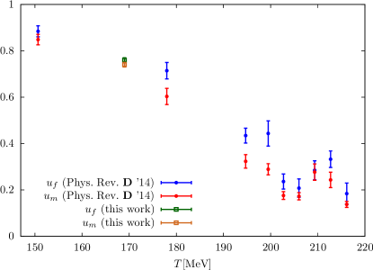
Figure 1: Comparison of the results obtained in [2] with this work [3]. Notice that in [2] the temperature scan was performed at a constant renormalized quark mass of $\overline{m}^{\overline{\text{MS}}}(\mu=2\text{GeV})\sim 15\text{MeV}$.

4 Axial-charge density correlator at ${\bf p}\neq{\bf 0}$

The relation between the Euclidean correlator $G_{A}(x_{0},T,{\bf p})$ and its spectral function is

$$G_{A}(x_{0},T,{\bf p})=\int^{\infty}_{0}d\omega~{}\rho^{A}(\omega,{\bf p})\frac{\cosh(\omega(\beta/2-x_{0}))}{\sinh(\omega\beta/2)}.$$ (8)

At finite temperature, the analysis of the correlator $G_{A}(x_{0},T,{\bf p})$ is more involved than at zero temperature: only at sufficiently small quark masses and momenta, and not too small $x_{0}$, is the correlator parametrically dominated by the pion pole. Therefore, we proceed by formulating a fit ansatz for the spectral function to take into account the non-pion contributions with the property that $\rho^{A}(\omega\to\infty,T,{\bf p})=\theta(\omega^{2}-4m^{2}-{\bf p}^{2})\frac{N_{c}}{24 \pi^{2}}({\bf p}^{2}+6m^{2})$ (see e.g. [12]). By integration with the kernel $\frac{\cosh(\omega(\beta/2-x_{0}))}{\sinh(\omega\beta/2)}$ the spectral function and the correlator fit ansätze read

$$\rho^{A}(\omega,{\bf p}) = A_{1}({\bf p})\sinh(\omega\beta/2)\delta(\omega-\omega_{\bf p})+A_{2}({\bf p})\frac{N_{c}}{24\pi^{2}}\left(1-e^{-\omega\beta}\right)\theta(\omega-c),$$ (9)

$$G_{A}(x_{0},T,{\bf p}) = A_{1}({\bf p})\cosh(\omega_{\bf p}(\beta/2-x_{0}))+A_{2}({\bf p})\frac{N_{c}}{24\pi^{2}}\left(\frac{e^{-cx_{0}}}{x_{0}}+\frac{e^{-c(\beta-x_{0})}}{\beta-x_{0}}\right).$$ (10)

The fit involves only 4 parameters but leaving $\omega_{\bf p}$ free led to poorly constrained fits. Therefore, we fix the value of $\omega_{\bf p}$ to the prediction of Eq. (1) with $u=u_{m}$ and ${\bf p}=(0,0,2\pi n/L)$ to see whether the data can be described in this way. Results are shown in Table 2. In view of the $\chi^{2}$-values, the data is consistent with this scenario. Moreover, the chiral effective theory makes a prediction for the residue of the retarded correlator at $\omega=\omega_{\bf p}$ reading (see App. B of [3])

$$\rho^{A}(\omega,{\bf p})=\underbrace{f^{2}_{\pi}(m^{2}_{\pi}+{\bf p}^{2})}_{\text{Res}(\omega_{\bf p})}\delta(\omega^{2}-\omega^{2}_{\bf p})+...$$ (11)

which can be written in terms of $A_{1}({\bf p})$ and a new parameter $b({\bf p})$ which parametrizes the deviation with respect to the chiral prediction

$$\text{Res}(\omega_{\bf p}) = 2A_{1}({\bf p})\omega_{\bf p}\sinh(\omega_{\bf p}\beta/2)$$ (12)

$$= f^{2}_{\pi}(m^{2}_{\pi}+{\bf p}^{2})(1+b({\bf p})).$$ (13)

In addition, we rescale the parameter $A_{2}({\bf p})\to\tilde{A}_{2}=A_{2}({\bf p})/{\bf p}^{2}$ (neglecting the quark mass which is parametrically small) whose natural value is 1. It turns out that indeed the parameter $b{(\bf p})$ is small for $n=1$ and the values of $\tilde{A}_{2}$ are of order one adding confidence to our description.

$n$	$A_{1}/T^{3}$	$\omega_{{\bf p}_{n}}/T$	$\tilde{A}_{2}$	$c/T$	$\text{Res}(\omega_{{\bf p}_{n}})/T^{4}$	$b$	$\chi^{2}/{\rm d.o.f}$
1	$2.95(4)\times 10^{-1}$	$2.19(3)$	$1.78(8)$	$6.7(3)$	$1.72(6)$	$-0.08(3)$	$0.06$
2	$1.40(5)\times 10^{-1}$	$3.73(6)$	$1.26(2)$	$6.1(1)$	$3.3(2)$	$-0.39(4)$	$0.15$
3	$4.9(3)\times 10^{-2}$	$5.40(9)$	$1.19(1)$	$7.7(1)$	$3.9(5)$	$-0.65(4)$	$0.35$
4	$1.7(2)\times 10^{-2}$	$7.1(1)$	$1.15(1)$	$9.67(9)$	$4.21(7)$	$-0.78(3)$	$0.49$
5	$4(1)\times 10^{-3}$	$8.8(1)$	$1.12(1)$	$11.7(1)$	$3(1)$	$-0.89(3)$	$1.04$

Table 2: Results of fits to the axial-charge density correlator at non-vanishing momentum ${\bf p}_{n}$. All errors quoted are statistical, and all renormalization factors are included. The quantity $\omega_{\bf p}/T$ is not a fit parameter; rather it is set to the value predicted by Eq. (1) with $u(T)=u_{m}=0.74(1)$.

5 Backus-Gilbert method on $G_{A}(x_{0},T,{\bf p})$

The Backus-Gilbert method (see [13, 14] for more recent studies) is a technique for inverting integral equations like Eq. (8) in order to directly obtain information on $\rho^{A}(\omega,{\bf p})$. The idea is to define an estimator

$$\hat{\rho}(\bar{\omega},{\bf p})=\int^{\infty}_{0}d\omega\;\hat{\delta}(\bar{\omega},\omega)\left(\frac{\rho_{A}(\omega,{\bf p})}{\tanh(\omega\beta/2)}\right)$$ (14)

where $\hat{\delta}(\bar{\omega},\omega)$ is called the resolution function which can be written in terms of a set of priori unknown coefficients $q_{i}(\bar{\omega})$ and the kernel functions $K_{i}(\omega)=\frac{\cosh(\omega(\beta/2-x^{i}_{0}))}{\cosh(\omega\beta/2)}$. It is a smooth function peaked around $\bar{\omega}$ which ”filters” the true spectral function. The coefficients $q_{i}(\bar{\omega})$ are determined by minimizing its width subject to the condition that the area is normalized to 1. During the process the matrix $W$ need to be inverted,

$$W_{ij}(\bar{\omega})=\lambda\left[\int^{\infty}_{0}d\omega K_{i}(\omega)(\omega-\bar{\omega})^{2}K_{j}(\omega)\right]+(1-\lambda)Cov(G_{i},G_{j}),\qquad 0<\lambda<1$$ (15)

where $Cov(G_{i},G_{j})$ denotes the $ij$-element of the covariance matrix of $G_{A}(x_{0},T,{\bf p})$. The parameter $\lambda$ controls the trade off between stability and resolution power. For values of $\lambda$ close to 1, the matrix is almost singular and the error on $\hat{\rho}(\bar{\omega})$ rapidly increases. Reducing the value of $\lambda$ improves stability at the cost of deteriorating the frequency resolution. Finally the solution reads

$$\hat{\rho}(\bar{\omega},{\bf p})=\sum_{i}q_{i}(\bar{\omega})G_{A}(x^{i}_{0},T,{\bf p}).$$ (16)

Notice that $\hat{\rho}(\bar{\omega},{\bf p})$ is a completely model independent estimator in the sense that no ansatz was needed for its calculation. Fig. 2 shows the estimators for different values of ${\bf p}$ and one already sees the good agreement in the high-frequency region with tree-level predictions.

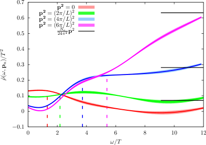
Figure 2: Estimators $\hat{\rho}(\omega,{\bf p}_{n})/T^{2}$ for $n=0,1,2,3$ together with its error shown as a band ($\lambda=0.002$). The vertical colored dashed lines correspond to the locations of the expected positions of the poles $\omega_{\bf p}$ according to Eq. (1) with $u(T)=u_{m}$. The black horizontal lines correspond to the treelevel asymptotic values of $\rho^{A}(\omega,{\bf p})$. All renormalization constants have been taken into account. Dimensionful quantities have been made dimensionless by the appropriate power of $T=1/24a$.

We can further check the agreement of $\text{Res}(\omega_{\bf p})$ with the chiral prediction by making use of $\hat{\rho}(\bar{\omega},{\bf p})$. Assuming a $\delta$-type excitation in $\rho^{A}$ we can write

$$\text{Res}(\omega_{\bf p},\omega)_{\text{BG}}=\frac{2\omega_{\bf p}\tanh(\omega_{\bf p}\beta/2)\hat{\rho}(\omega,{\bf p})}{\hat{\delta}(\omega,\omega_{\bf p})}$$ (17)

where we use $\omega_{\bf p}$ as input according to Eq. (1) with $u(T)=u_{m}$. This defines a function of $\omega$. The natural choice where $\text{Res}(\omega_{\bf p},\omega)_{\text{BG}}$ is expected to be the best estimator for the true residue is at $\omega\approx\omega_{\bf p}$. By looking at Fig. 3 we see that approximately around this value the curve intercepts the grey band which represents the chiral prediction and therefore confirms the validity of Eq. (1) at least up to ${\bf p}=400\text{MeV}$ ($n=1$).

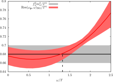
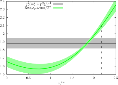
Figure 3: The effective residue $\text{Res}(\omega_{\bf p},\omega)_{\text{BG}}$ as defined in Eq. (17). Left: No momentum induced, ${\bf p}=0$. Right: One unit of momentum induced, ${\bf p}_{1}=(0,0,2\pi/L)$. The grey band is the expectation in terms of screening quantities. All renormalization factors are included. The errors arise from the statistical uncertainty. The values of $\omega_{\bf p}$ are indicated by dashed vertical lines.

6 Conclusions

We have successfully tested the dispersion relation of Eq. (1) for the pion quasiparticle by performing direct fits to $G_{A}(x_{0},T,{\bf p})$ (alternatively applying the Backus-Gilbert method) using the value of the parameter $u$ determined at zero momentum. Table 1 indicates that the pion mass ”splits” at finite temperature into a lower pole mass and a higher screening mass. Our findings are in qualitative agreement with two-loop calculation in ChPT (see eg. [15, 16]). Both suggest a violation of boost invariance due to the presence of the medium. Although $N_{\tau}=24$ is at the current state of the art concerning thermal ensembles, finite volume effects as well as lattice artifacts should be investigated. Our plans for the future are to simulate at the physical value of the light quark mass and/or to include the strange quark.

- [1] A. Bazavov et al. (HotQCD Collaboration), Phys. Rev. D86, 034509 (2012) [arXiv:1203.0784].
- [2] Bastian B. Brandt, Anthony Francis, Harvey B. Meyer, and Daniel Robaina, Phys. Rev. D90, 054509 (2014) [arXiv:1406.5602].
- [3] Bastian B. Brandt, Anthony Francis, Harvey B. Meyer, and Daniel Robaina, (2015) [arXiv:1506.05732].
- [4] G. Backus and F. Gilbert, Geophysical Journal of the Royal Astronomical Society 16, 169205 (1968).
- [5] G. Backus and F. Gilbert, Philosophical Transactions of the Royal Society of London A: Mathematical, Physical and Engineering Sciences 266, 123-192 (1970).
- [6] D. Teaney, Phys. Rev. D74 (2006) 045025 [arXiv:hep-ph/0602044].
- [7] D. T. Son and M. A. Stephanov, Phys. Rev. Lett. 88, 202302 (2002) [arXiv:hep-ph/0111100].
- [8] D. T. Son and M. A. Stephanov, Phys. Rev. D66, 076011 (2002) [arXiv:hep-ph/0204226].
- [9] M. Bochicchio, L. Maiani, G. Martinelli, G. C. Rossi, and M. Testa, Nucl. Phys. B262, 331 (1985).
- [10] B. B. Brandt, A. Francis, H. B. Meyer, O. Philipsen, and H. Wittig (2013) [arXiv:1310.8326].
- [11] Patrick Fritzsch et al., Nucl. Phys. B865, 397-429 (2012) [arXiv:1205.5380].
- [12] Gert Aarts and Jose M. Martinez Resco, Nucl. Phys. B726, 93-108 (2005) [arXiv:hep-lat/0507004].
- [13] H. Haarioa and E. Somersalo, Numerical Functional Analysis and Optimization 9, 917-943 (1987).
- [14] A. Kirsch, B Schomburg, and G Berendt, Inverse Problems 4, 771 (1988).
- [15] A. Schenk, Phys. Rev. D47, 5138-5155 (1993).
- [16] D. Toublan, Phys. Rev. D56, 5629-5645 (1997) [arXiv:hep-ph/9706273].