The geometrically nonlinear Cosserat micropolar shear-stretch energy. Part II: Non-classical energy-minimizing microrotations in 3D and their computational validation

Dedicated to Gianfranco Capriz on the occasion of his 90th birthday:
– we bow in great admiration to his lifetime achievement! –

Abstract

In any geometrically nonlinear, isotropic and quadratic Cosserat micropolar extended continuum model formulated in the deformation gradient field $F\coloneqq\nabla\varphi:\Omega\to\operatorname{GL}^{+}(n)$ and the microrotation field $R:\Omega\to\operatorname{SO}(n)$, the shear–stretch energy is necessarily of the form

$$\operatorname{W_{\mu,\mu_{c}}}(R\,;F) \coloneqq\mu\left\lVert\operatorname{sym}(R^{T}F-{\boldsymbol{\mathbbm{1}}})\right\rVert^{2}+\mu_{c}\left\lVert\operatorname{skew}(R^{T}F-{\boldsymbol{\mathbbm{1}}})\right\rVert^{2}\;.$$

We aim at the derivation of closed form expressions for the minimizers of $\operatorname{W_{\mu,\mu_{c}}}(R\,;F)$ in $\operatorname{SO}(3)$, i.e., for the set of optimal Cosserat microrotations in dimension $n\!=\!3$, as a function of $F\in\operatorname{GL}^{+}(n)$. In a previous contribution (Part I), we have first shown that, for all $n\geq 2$, the full range of weights $\mu>0$ and $\mu_{c}\geq 0$ can be reduced to either a classical or a non-classical limit case. We have then derived the associated closed form expressions for the optimal planar rotations in $\operatorname{SO}(2)$ and proved their global optimality. In the present contribution (Part II), we characterize the non-classical optimal rotations in dimension $n\!=\!3$. After a lift of the minimization problem to the unit quaternions, the Euler–Lagrange equations can be symbolically solved by the computer algebra system Mathematica. Among the symbolic expressions for the critical points, we single out two candidates $\operatorname{rpolar}^{\pm}_{\mu,\mu_{c}}(F)\in\operatorname{SO}(3)$ which we analyze and for which we can computationally validate their global optimality by Monte Carlo statistical sampling of $\operatorname{SO}(3)$. Geometrically, our proposed optimal Cosserat rotations $\operatorname{rpolar}^{\pm}_{\mu,\mu_{c}}(F)$ act in the “plane of maximal strain” and our previously obtained explicit formulae for planar optimal Cosserat rotations in $\operatorname{SO}(2)$ reveal themselves as a simple special case. Further, we derive the associated reduced energy levels of the Cosserat shear–stretch energy and criteria for the existence of non-classical optimal rotations.

Key words: Cosserat, Grioli’s theorem, micropolar, polar media, rotations, quaternions, Lagrange multiplier, equality constraints, non-symmetric stretch, Cosserat couple modulus, polar decomposition.

AMS 2010 subject classification: 15A24, 22E30, 74A30, 74A35, 74B20, 74G05, 74G65, 74N15.

1 Introduction

In this second part (Part II) of a series, we consider the weighted optimality problem for the Cosserat shear–stretch energy $\operatorname{W_{\mu,\mu_{c}}}:\;\operatorname{SO}(n)\,\times\,\operatorname{GL}^{+}(n)\to\operatorname{\sideset{}{{}_{0}^{+}}{\operatorname{\mathbb{R}}}}$,

$$\operatorname{W_{\mu,\mu_{c}}}(R\,;F)\;\coloneqq\;\mu\,\left\lVert\operatorname{sym}(R^{T}F-{\boldsymbol{\mathbbm{1}}})\right\rVert^{2}\,+\,\mu_{c}\,\left\lVert\operatorname{skew}(R^{T}F-{\boldsymbol{\mathbbm{1}}})\right\rVert^{2}\;.$$ (1.1)

The arguments are the deformation gradient field $F\coloneqq\nabla\varphi:\Omega\to\operatorname{GL}^{+}(n)$ and the microrotation field $R:\Omega\to\operatorname{SO}(n)$ evaluated at a given point of the domain $\Omega$. This energy arises in any geometrically nonlinear, isotropic and quadratic Cosserat micropolar continuum model. Note that it is always possible to express the local energy contribution in a Cosserat model as $W=W(\overline{U})$, where $\overline{U}\coloneqq R^{T}F$ is the first Cosserat deformation tensor. This reduction follows from objectivity requirements and has already been observed by the Cosserat brothers [17, p. 123, eq. (43)], see also [28] and [52]. Since $\overline{U}$ is in general non-symmetric, the most general isotropic and quadratic local energy contribution which is zero at the reference state is given by

$$\underbrace{\mu\,\left\lVert\operatorname{sym}(\overline{U}-{\boldsymbol{\mathbbm{1}}})\right\rVert^{2}\,+\,\mu_{c}\,\left\lVert\operatorname{skew}(\overline{U}-{\boldsymbol{\mathbbm{1}}})\right\rVert^{2}}_{\text{``shear--stretch energy''}}\quad+\quad\underbrace{\frac{\lambda}{2}\,{\operatorname{tr}\left[{\overline{U}-{\boldsymbol{\mathbbm{1}}})}\right]}^{2}}_{\text{``volumetric energy''}}\;.$$ (1.2)

The last term will be discarded in the following, since it couples the rotational and volumetric response, a feature not present in the well-known isotropic linear Cosserat models.

Let us now proceed to the primary objective of our present contribution

Problem 1.1 (Weighted optimality in dimension $n=3$).

Let $\mu>0$ and $\mu_{c}\geq 0$. Compute the set of optimal rotations

$$\mathchoice{\underset{R\,\in\,\operatorname{SO}(3)}{\operatorname{arg\,min}}\,{\operatorname{W_{\mu,\mu_{c}}}(R\,;F)}}{\operatorname{arg\,min}_{R\,\in\,\operatorname{SO}(3)}\,{\operatorname{W_{\mu,\mu_{c}}}(R\,;F)}}{}{}\;\coloneqq\;\mathchoice{\underset{R\,\in\,\operatorname{SO}(3)}{\operatorname{arg\,min}}\,{\left\{\mu\,\left\lVert\operatorname{sym}(R^{T}F-{\boldsymbol{\mathbbm{1}}})\right\rVert^{2}\,+\,\mu_{c}\,\left\lVert\operatorname{skew}(R^{T}F-{\boldsymbol{\mathbbm{1}}})\right\rVert^{2}\right\}}}{\operatorname{arg\,min}_{R\,\in\,\operatorname{SO}(3)}\,{\left\{\mu\,\left\lVert\operatorname{sym}(R^{T}F-{\boldsymbol{\mathbbm{1}}})\right\rVert^{2}\,+\,\mu_{c}\,\left\lVert\operatorname{skew}(R^{T}F-{\boldsymbol{\mathbbm{1}}})\right\rVert^{2}\right\}}}{}{}$$ (1.3)

for given parameter $F\in\operatorname{GL}^{+}(3)$ with distinct singular values $\sigma_{1}>\sigma_{2}>\sigma_{3}>0$.

We use the notation $\operatorname{sym}(X)\coloneqq\frac{1}{2}(X+X^{T})$, $\operatorname{skew}(X)\coloneqq\frac{1}{2}(X-X^{T})$, $\big{<}X,\,Y\big{>}\coloneqq{\operatorname{tr}\left[{X^{T}Y}\right]}$ and we denote the induced Frobenius matrix norm by $\left\lVert X\right\rVert^{2}\coloneqq\big{<}X,\,X\big{>}=\sum_{1\leq i,j\leq n}X_{ij}^{2}$. In mechanics applications, the weights $\mu>0$ and $\mu_{c}\geq 0$ can be identified with the Lamé shear modulus $\mu>0$ from linear elasticity and the so-called Cosserat couple modulus $\mu_{c}\geq 0$. The parameter $\lambda$ in the most general form of the energy (1.2) can further be identified with the second Lamé parameter. Note that the interpretation of the Cosserat couple modulus $\mu_{c}$ is somewhat delicate, see, e.g., [60], which is one of the fundamental motivations for this second contribution in a series.

In Part I of this paper [29], we have proved a still surprising reduction lemma [29, Lem. 2.2, p. 4] for the material parameters (weights) $\mu$ and $\mu_{c}$ which is valid for all space dimensions $n\geq 2$. This lemma singles out a classical parameter range $\mu_{c}\geq\mu>0$ and a non-classical parameter range $\mu_{c}\geq\mu>0$ for $\mu$ and $\mu_{c}$ and reduces both ranges to an associated limit case. The classical limit case is given by $(\mu,\mu_{c})=(1,1)$ and the non-classical limit case is given by $(\mu,\mu_{c})=(1,0)$. We then apply the parameter reduction [29, Lem. 2.2, p. 4] to Problem 1.1 and solve it in dimension $n=2$. This allows us to discuss the optimal planar Cosserat rotations and we observe that the classical and the non-classical parameter ranges for $\mu$ and $\mu_{c}$ characterize two substantially different types of optimal Cosserat rotations.

To explain this difference, we first need to introduce the polar factor $\operatorname{R_{\rm p}}(F)\in\operatorname{SO}(n)$ which is obtained from the right polar decomposition $F=\operatorname{R_{\rm p}}(F)\,U(F)$ of the deformation gradient $F\in\operatorname{GL}^{+}(n)$. Here, $U(F)\coloneqq\sqrt{F^{T}F}\in{\rm{PSym}}(n)$ denotes the positive definite symmetric right Biot-stretch tensor. We recall that the eigenvalues of $U\in{\rm{PSym}}(n)$ are by definition the singular values $\sigma_{1}>\sigma_{2}>\sigma_{3}>0$ of the deformation gradient $F\in\operatorname{GL}^{+}(n)$.

In the classical parameter range $\mu_{c}\geq\mu>0$, the polar factor $\operatorname{R_{\rm p}}$ admits a variational characterization which is noteworthy in its own right: namely, for all $n\geq 2$, it is the unique minimizer for (1.1) as a generalized version of Grioli’s theorem shows, see [35, 50, 69], or [29, Cor. 2.4, p. 5]. This variational characterization of the polar factor inspired us to introduce the following

Definition 1.2 (Relaxed polar factor(s)).

Let $\mu>0$ and $\mu_{c}\geq 0$. We denote the set-valued mapping that assigns to a given parameter $F\in\operatorname{GL}^{+}(n)$ its associated set of energy-minimizing rotations by rpolar_μ,μ_c(F)  ≔  .

In dimensions $k=2,3$, we denote the associated optimal Cosserat rotation angles by $\alpha_{\mu,\mu_{c}}(F)\subset(-\pi,\pi]$. More generally, in what follows, we shall denote the rotation angle of the (absolute) rotation field $R\in\operatorname{SO}(k)$ by $\alpha\in(-\pi,\pi]$ and the rotation axis by $r\in\mathbb{S}^{k-1}$. By $\mathbb{S}^{n-1}\subset\operatorname{\mathbb{R}}^{n}$, we denote the unit $n-1$-sphere. In dimension $k=3$, we use the well-known axis-angle parametrization of rotations which we write as $[\alpha,\,r^{T}]$.

Since the classical parameter domain $\mu_{c}\geq\mu>0$ is very well understood by now, we can focus on the non-classical parameter range $\mu>\mu_{c}\geq 0$ in our efforts to solve Problem 1.1. Here, the parameter reduction lemma [29, Lem. 2.2, p. 4] allows us to restrict our attention to the non-classical limit case $(\mu,\mu_{c})=(1,0)$, because it shows the equivalence

$$\mathchoice{\underset{R\,\in\,\operatorname{SO}(n)}{\operatorname{arg\,min}}\,{W_{\mu,\mu_{c}}(R\,;F)}}{\operatorname{arg\,min}_{R\,\in\,\operatorname{SO}(n)}\,{W_{\mu,\mu_{c}}(R\,;F)}}{}{}\quad=\quad\mathchoice{\underset{R\,\in\,\operatorname{SO}(n)}{\operatorname{arg\,min}}\,{W_{1,0}(R\,;\widetilde{F}_{\mu,\mu_{c}})}}{\operatorname{arg\,min}_{R\,\in\,\operatorname{SO}(n)}\,{W_{1,0}(R\,;\widetilde{F}_{\mu,\mu_{c}})}}{}{}$$ (1.4)

for all $n\geq 2$. On the right hand side appears the rescaled deformation gradient $\widetilde{F}_{\mu,\mu_{c}}\coloneqq\lambda^{-1}_{\mu,\mu_{c}}\cdot F\in\operatorname{GL}^{+}(n)$ which is obtained from $F\in\operatorname{GL}^{+}(n)$ by multiplication with the inverse of the induced scaling parameter $\lambda_{\mu,\mu_{c}}\coloneqq\frac{\mu}{\mu-\mu_{c}}>0$. We note that we use the previous notation throughout the text and further introduce the singular radius $\rho_{\mu,\mu_{c}}\coloneqq\frac{2\mu}{\mu-\mu_{c}}$.

It follows that the set of optimal Cosserat rotations can be described by

$$\operatorname{rpolar}_{\mu,\mu_{c}}(F)\;=\;\operatorname{rpolar}_{1,0}(\widetilde{F}_{\mu,\mu_{c}})$$ (1.5)

for the entire non-classical parameter range $\mu>\mu_{c}\geq 0$. This simplifies our main objective Problem 1.1 considerably, since it suffices now to solve

Problem 1.3 (Weighted optimality in the non-classical limit case $(\mu,\mu_{c})=(1,0)$).

Let $\mu>0$ and $\mu_{c}\geq 0$. Compute the set of optimal rotations

$$\mathchoice{\underset{R\,\in\,\operatorname{SO}(3)}{\operatorname{arg\,min}}\,{\operatorname{W_{1,0}}(R\,;F)}}{\operatorname{arg\,min}_{R\,\in\,\operatorname{SO}(3)}\,{\operatorname{W_{1,0}}(R\,;F)}}{}{}\;\coloneqq\;\mathchoice{\underset{R\,\in\,\operatorname{SO}(3)}{\operatorname{arg\,min}}\,{\left\lVert\operatorname{sym}(R^{T}F-{\boldsymbol{\mathbbm{1}}})\right\rVert^{2}}}{\operatorname{arg\,min}_{R\,\in\,\operatorname{SO}(3)}\,{\left\lVert\operatorname{sym}(R^{T}F-{\boldsymbol{\mathbbm{1}}})\right\rVert^{2}}}{}{}$$ (1.6)

for given parameter $F\in\operatorname{GL}^{+}(3)$ with distinct singular values $\sigma_{1}>\sigma_{2}>\sigma_{3}>0$.

Regarding our Problem 1.3 at hand, we will see in Section 2 that there are in general two energy-minimizing solutions with a certain symmetry. They both have the same rotation axis but differ by the sign of their respective rotation angles which allows us to select the corresponding branches by that sign. Accordingly, we introduce the notations $\operatorname{rpolar}^{\pm}_{\mu,\mu_{c}}(F)$ and $\alpha^{\pm}_{\mu,\mu_{c}}(F)$. Loosely spoken, we will see that the optimal Cosserat rotations coincide with the polar factor $\operatorname{R_{\rm p}}$ in a certain compressive regime for $F\in\operatorname{GL}^{+}(3)$, but deviate in a certain expansive regime. We shall precisely characterize this in terms of the singular radius $\operatorname{\rho_{\mu,\,\mu_{c}}}$. Such a material behavior is commonly referred to as a tension-compression asymmetry which is an interesting natural phenomenon studied in the material sciences, see, e.g., [33, 32] and [81] for experimental studies of nickel titanium (NiTi) shape memory single crystals for a glimpse on this broad subject.

Problem 1.3 is a minimization problem on the matrix Lie group $\operatorname{SO}(3)$ of special orthogonal matrices parameterized by the deformation gradient $F\in\operatorname{GL}^{+}(3)$ in the identity component of the general linear group. Although it is not our duty, we want to point to some valuable introductory references to this subject. An excellent general reference for minimization problems on manifolds is the text by Absil, Mahony and Sepulchre [1]. There, also numerical solution approaches are presented. For an introduction to Lie groups and matrix groups, we refer to, e.g., [3, 47] and [41]. For compact Lie groups and their representation theory, see, e.g., [42] and [10]. There is also a growing body of closely related work treating minimization problems on matrix groups and Grioli’s theorem in a similar context [71, 69, 44, 70].

Instead of turning towards the solution of Problem 1.3 right away, we take a step back and notice that there is still another opportunity for simplification which reduces the space of parameters $F\in\operatorname{GL}^{+}(3)$ to the space of ordered singular values $\sigma_{1}\geq\sigma_{2}\geq\sigma_{3}>0$ of $F$. This can be achieved by a principal axis transformation which introduces a relative rotation $\widehat{R}$ and allows us to introduce

Definition 1.4 (Cosserat shear–stretch energy for the relative rotation $\widehat{R}$).

Let $\mu>0$, $\mu_{c}\geq 0$ and let $D\coloneqq\operatorname{diag}(\sigma_{1},\sigma_{2},\sigma_{3})$ with $\sigma_{1}>\sigma_{2}>\sigma_{3}>0$ the singular values of $F\in\operatorname{GL}^{+}(3)$. The energy of the relative rotation $\widehat{R}\in\operatorname{SO}(3)$ is given by

$$\widehat{W}_{\mu,\mu_{c}}(\widehat{R}\,;D)\;\coloneqq\;W_{\mu,\mu_{c}}(\widehat{R}^{T}\,;D)\;\coloneqq\;\mu\;\left\lVert\operatorname{sym}(\widehat{R}D-{\boldsymbol{\mathbbm{1}}})\right\rVert^{2}+\mu_{c}\;\left\lVert\operatorname{skew}(\widehat{R}D-{\boldsymbol{\mathbbm{1}}})\right\rVert^{2}\;.$$ (1.7)

This transformation is described in Section 2 and leads us to the reduced

Problem 1.5 (Optimality of relative rotations in dimension $n=3$).

Let $\mu=1$ and $\mu_{c}=0$. Compute the set of optimal relative rotations

$$\mathchoice{\underset{\widehat{R}\,\in\,\operatorname{SO}(3)}{\operatorname{arg\,min}}\,{\widehat{W}_{1,0}(\widehat{R}\,;D)}}{\operatorname{arg\,min}_{\widehat{R}\,\in\,\operatorname{SO}(3)}\,{\widehat{W}_{1,0}(\widehat{R}\,;D)}}{}{}\quad=\quad\mathchoice{\underset{\widehat{R}\,\in\,\operatorname{SO}(3)}{\operatorname{arg\,min}}\,{\left\lVert\operatorname{sym}(\widehat{R}\operatorname{diag}(\sigma_{1},\sigma_{2},\sigma_{3})-{\boldsymbol{\mathbbm{1}}})\right\rVert^{2}}}{\operatorname{arg\,min}_{\widehat{R}\,\in\,\operatorname{SO}(3)}\,{\left\lVert\operatorname{sym}(\widehat{R}\operatorname{diag}(\sigma_{1},\sigma_{2},\sigma_{3})-{\boldsymbol{\mathbbm{1}}})\right\rVert^{2}}}{}{}$$ (1.8)

for a given diagonal matrix $D\coloneqq\operatorname{diag}(\sigma_{1},\sigma_{2},\sigma_{3})$ with $\sigma_{1}>\sigma_{2}>\sigma_{3}>0$ the ordered singular values of the deformation gradient $F\in\operatorname{GL}^{+}(3)$.

In this text, we strive to mark quantities related to relative rotations with a “hat”-symbol, e.g., we write $\widehat{R}\in\operatorname{SO}(3)$. Further, we note that although, for now, we explicitly exclude the case of multiple singular values of $F$ from our analysis, there is no major obstruction. The technical treatment would, however, clutter our exposition of the basic mechanisms which we want to distill here.

At present, an explicit formal solution for the three-dimensional problem (let alone the $n$-dimensional problem) seems out of reach for us. We have, however, successfully computed explicit formulae for the critical points of the Cosserat shear–stretch energy by the use of computer algebra from which we have determined optimal solutions. For this approach to succeed, we first lift the Cosserat shear–stretch energy expressed in principal axis coordinates to the sphere of unit quaternions $\mathbb{S}^{3}\subset\operatorname{\mathbb{H}}$ and subsequently apply the Lagrange multiplier technique for minimization with equality constraints, see, e.g., [39]. The unit quaternions form a two-sheeted cover of $\operatorname{SO}(3)$ and allow for a convenient representation of rotations in three-space. For a preceding successful application of quaternions to represent the rotational degress of freedom in Cosserat theory, see, e.g., [56]. A highly interesting recent approach to Cosserat shell theory which also uses quaternions is based on geodesic finite elements, see [77] and [36, 76].

This paper is now structured as follows: in Section 2, we introduce the lift of the Cosserat shear–stretch energy from $\operatorname{SO}(3)$ to the sphere of unit quaternions $\mathbb{S}^{3}\subset\operatorname{\mathbb{H}}\cong\operatorname{\mathbb{R}}^{4}$. We then state the corresponding Euler–Lagrange equations and present the energy-minimizing solutions. The complete set of critical points computed by Mathematica [88] is provided in Appendix A. In Section 3, we present a geometric interpretation of the optimal Cosserat rotations $\operatorname{rpolar}^{\pm}_{\mu,\mu_{c}}(F)$ in terms of the maximal mean planar stretch $u^{\rm mmp}$ for the entire non-classical parameter range $\mu>\mu_{c}\geq 0$. This leads us to introduce a classical and a non-classical domain for the parameter $F\in\operatorname{GL}^{+}(3)$ for which we also derive some interesting alternative criteria. This illuminates the bifurcation behavior of $\operatorname{rpolar}_{\mu,\mu_{c}}(F)$. Further, we compute the associated reduced energy levels $W^{\rm red}_{\mu,\mu_{c}}(F)$ for the Cosserat shear–stretch energy. Then in Section 4, we shed light on our methodology for the analysis of the critical points and the experimental computational validation of the energy-minimizing Cosserat rotations using statistical (Monte Carlo) methods. Finally, we summarize our findings in a short conclusion presented in Section 5.

2 Solvable Euler-Lagrange equations: transformation, lift and Lagrange multipliers

In this section, we use a classical result from the representation theory of compact Lie groups to cast the reduced minimization problem stated as Problem 1.5 into a form which allows us to symbolically compute explicit expressions for the critical points using Mathematica.

It is well-known that the Lie group of unit quaternions $\mathbb{S}^{3}\subset\operatorname{\mathbb{H}}\cong\operatorname{\mathbb{R}}^{4}$ is closely related to the matrix group of rotations $\operatorname{SO}(3)$, see, e.g., [49] or [34, Chap. 9]. More precisely, the unit quaternions $\mathbb{S}^{3}$ form a double cover of the matrix group $\operatorname{SO}(3)$. For a general introduction to analysis on smooth manifolds which includes smooth coverings, see, e.g., [47]. For a dynamical systems approach to quaternions, see, e.g., [72] which nicely demonstrates the usefulness of quaternions for mechanics applications with constraints. A more algebraic approach to quaternions with historical remarks is given in [25], and, finally, for those who enjoy the classics, see [37] and [38].

2.1 Transformation into principal directions

In order to reduce the parameter space $\operatorname{GL}^{+}(3)$, we use the (unique) polar decomposition $F=\operatorname{R_{\rm p}}U$ and the (non-unique) spectral decomposition of $U=\sqrt{F^{T}F}\in{\rm{PSym}}(3)$ given by $U=QDQ^{T}$, $Q\in\operatorname{SO}(3)$, and expand

$$R^{T}F=R^{T}\operatorname{R_{\rm p}}U=R^{T}\operatorname{R_{\rm p}}QDQ^{T}\;.$$ (2.1)

Here, the diagonal matrix $D=\operatorname{diag}(\sigma_{1},\sigma_{2},\sigma_{3})$ contains the eigenvalues of $U$ on its diagonal. These are precisely the singular values of $F\in\operatorname{GL}^{+}(3)$. In fact, this is a particular form of the singular value decomposition (SVD). If $F$ has only simple singular values, then it is always possible to choose the rotation $Q$ such that an ordering $\sigma_{1}>\sigma_{2}>\sigma_{3}>0$ is achieved.

Exploiting that $Q\in\operatorname{SO}(3)$, it is now possible to carry out a transformation of the Cosserat shear–stretch energy into principal axis coordinates – essentially due to isotropy of the energy. For the actual computation, note first that

$$Q^{T}(\operatorname{sym}(R^{T}F)-{\boldsymbol{\mathbbm{1}}})Q=Q^{T}\left(\operatorname{sym}(R^{T}\operatorname{R_{\rm p}}QDQ^{T})-{\boldsymbol{\mathbbm{1}}})\right)Q$$

$$\quad=\operatorname{sym}(Q^{T}R^{T}\operatorname{R_{\rm p}}QDQ^{T}Q-Q^{T}Q)=\operatorname{sym}(\underbrace{Q^{T}R^{T}\operatorname{R_{\rm p}}Q}_{\eqqcolon\;\widehat{R}}D-{\boldsymbol{\mathbbm{1}}})=\operatorname{sym}(\widehat{R}D-{\boldsymbol{\mathbbm{1}}})\;.$$ (2.2)

In the process, it is natural to introduce the rotation

$$\widehat{R}\coloneqq Q^{T}R^{T}\operatorname{R_{\rm p}}Q$$ (2.3)

which acts relative to the polar factor $\operatorname{R_{\rm p}}$ in the coordinate system induced by the columns of $Q$, i.e., in a positively oriented frame of principal directions of $U$. This interpretation is also nicely illustrated by the inverse formula

$$R=\left(Q\widehat{R}Q^{T}\operatorname{R_{\rm p}}^{T}\right)^{T}=\operatorname{R_{\rm p}}Q\widehat{R}^{T}Q^{T}$$ (2.4)

which allows to recover the original absolute rotation $R$ from the relative rotation $\widehat{R}$. Our next step is to insert the transformed symmetric part $\eqref{eq:symtransform}$ into the definition of

$$W_{1,0}(R\,;F)=\left\lVert\operatorname{sym}(R^{T}F-{\boldsymbol{\mathbbm{1}}})\right\rVert^{2}=\left\lVert Q^{T}\operatorname{sym}(R^{T}F-{\boldsymbol{\mathbbm{1}}})Q\right\rVert^{2}=\left\lVert\operatorname{sym}(\widehat{R}D-{\boldsymbol{\mathbbm{1}}})\right\rVert^{2}\;,$$ (2.5)

where we have used that the conjugation by $Q^{T}$ preserves the Frobenius matrix norm.

This is a promising simplification of the Cosserat shear–stretch energy, because it reduces the dimension of the parameter space from $\dim\operatorname{GL}^{+}(3)=9$ to only $3$ parameters. However, we still have to account for the non-uniqueness of $Q$. To this end, we introduce the following symmetric rotation matrices

$$Q_{1}\coloneqq{\boldsymbol{\mathbbm{1}}},\quad Q_{2}\coloneqq\operatorname{diag}(1,-1,-1),\quad Q_{3}\coloneqq\operatorname{diag}(-1,1,-1),\quad Q_{4}\coloneqq\operatorname{diag}(-1,-1,1)\;,$$

and collect them in a set $\mathcal{S}\coloneqq\left\{Q_{1},Q_{2},Q_{3},Q_{4}\right\}\subset\operatorname{SO}(3)$. This set forms a discrete subgroup of $\operatorname{SO}(3)$ which is isomorphic to the Klein four-group $K_{4}\cong\mathbb{Z}^{2}\times\mathbb{Z}^{2}$, as is easily inferred by a comparison of the multiplication tables.

Remark 2.1 (Uniqueness of the factor $Q$).

Let $\sigma_{1}>\sigma_{2}>\sigma_{3}>0$ be the ordered eigenvalues of $U\coloneqq\sqrt{F^{T}F}$ and let $D\coloneqq\operatorname{diag}(\sigma_{1},\sigma_{2},\sigma_{3})$. It is well-known that the factor $Q\in\operatorname{SO}(3)$ in the spectral decomposition $U=QDQ^{T}$ is only determined up to the choice of a right handed orientation of the uniquely determined orthogonal eigenspaces of $U$. This corresponds to the products $QS$, $S\in\mathcal{S}$, which represent all of these possibilities.

It is easy to see that for any possible choice of right handed orientation encoded by $S\in\mathcal{S}$, we obtain the same energy level

$$\left\lVert\operatorname{sym}(\widehat{R}D-{\boldsymbol{\mathbbm{1}}})\right\rVert^{2}\;=\;\left\lVert\operatorname{sym}(\widehat{R}SDS^{T}-{\boldsymbol{\mathbbm{1}}})\right\rVert^{2}\;=\;\left\lVert\operatorname{sym}(S^{T}\widehat{R}SD-{\boldsymbol{\mathbbm{1}}})\right\rVert^{2}\$$ (2.6)

which implies

$$\mathchoice{\underset{\widehat{R}\,\in\,\operatorname{SO}(3)}{\operatorname{arg\,min}}\,{W_{1,0}(\widehat{R}^{T}\,;D)}}{\operatorname{arg\,min}_{\widehat{R}\,\in\,\operatorname{SO}(3)}\,{W_{1,0}(\widehat{R}^{T}\,;D)}}{}{}\;=\;\{\,S^{T}\widehat{R}S\,\;|\;R\in\mathchoice{\underset{\widehat{R}\,\in\,\operatorname{SO}(3)}{\operatorname{arg\,min}}\,{W_{1,0}(\widehat{R}^{T}\,;D)}}{\operatorname{arg\,min}_{\widehat{R}\,\in\,\operatorname{SO}(3)}\,{W_{1,0}(\widehat{R}^{T}\,;D)}}{}{}\;\text{and}\;S\in\mathcal{S}\}\;.$$ (2.7)

Thus, $\mathcal{S}$ is a symmetry group of the set of energy-minimizing rotations which acts by conjugation. The previous analysis reveals that the non-uniqueness of $Q\in\operatorname{SO}(3)$ is not an issue for the minimization problem, since all possible choices $QS$, $S\in\mathcal{S}$, lead to the same energy level.

Without any loss of generality, we may henceforward focus on the solution of

$$\mathchoice{\underset{\widehat{R}\in\operatorname{SO}(3)}{\operatorname{arg\,min}}\,{\left\lVert\operatorname{sym}(\widehat{R}D-{\boldsymbol{\mathbbm{1}}})\right\rVert^{2}}}{\operatorname{arg\,min}_{\widehat{R}\in\operatorname{SO}(3)}\,{\left\lVert\operatorname{sym}(\widehat{R}D-{\boldsymbol{\mathbbm{1}}})\right\rVert^{2}}}{}{}\quad=\quad\mathchoice{\underset{\widehat{R}\in\operatorname{SO}(3)}{\operatorname{arg\,min}}\,{W_{1,0}(\widehat{R}^{T}\,;D)}}{\operatorname{arg\,min}_{\widehat{R}\in\operatorname{SO}(3)}\,{W_{1,0}(\widehat{R}^{T}\,;D)}}{}{}\;.$$ (2.8)

This proves the reduction of Problem 1.1 to the minimization problem described in Problem 1.5 in Section 1 for the non-classical limit case $(\mu,\mu_{c})=(1,0)$. The same principal axes transformation can also be carried out for arbitrary values of $\mu$ and $\mu_{c}$ which gives rise to Definition 1.4.

In what follows, we denote the rotation angle of the (absolute) microrotation field $R\in\operatorname{SO}(3)$ by $\alpha\in(-\pi,\pi]$ and the axis of the rotation by $r\in\mathbb{S}^{2}$, where $\mathbb{S}^{n}\subset\operatorname{\mathbb{R}}^{n+1}$ denotes the unit $n$-sphere. This leads us to the axis-angle representation of a rotation which we write as $[\alpha,\,r^{T}]$. In what follows, we work with different parametrizations of the group of rotations $\operatorname{SO}(3)$ simultaneously. Thus, we introduce the symbol $\equiv$ in order to identify rotations in $\operatorname{SO}(3)$ which are described with respect to different parametrizations of $\operatorname{SO}(3)$. For example, we might write for the relative rotation $\widehat{R}\equiv[\hat{\beta},\,(\hat{r}_{1},\hat{r}_{2},\hat{r}_{3})]$ and for a unit quaternion $q\in\mathbb{S}^{3}$ describing $R\in\operatorname{SO}(3)$, we have $q\equiv R\equiv-q$. We see that, in general, this binary relation is not unique since the parametrizations need not be one-to-one.

The symmetry group $\mathcal{S}\coloneqq\left\{Q_{1},Q_{2},Q_{3},Q_{4}\right\}$ hints at the structure of the set of optimal relative Cosserat rotations. In our previously introduced notation, we find:

$$Q_{1}^{T}\widehat{R}Q_{1} \,\equiv\,\left[\hat{\beta},\,(\hat{r}_{1},\hat{r}_{2},\hat{r}_{3})\right]\,,\quad \quad Q_{2}^{T}\widehat{R}Q_{2}\,\equiv\,\left[\hat{\beta},\,(\hat{r}_{1},-\hat{r}_{2},-\hat{r}_{3})\right]\,,$$ (2.9)

$$Q_{3}^{T}\widehat{R}Q_{3} \,\equiv\,\left[\hat{\beta},\,(-\hat{r}_{1},\hat{r}_{2},-\hat{r}_{3})\right]\,,\quad \quad Q_{4}^{T}\widehat{R}Q_{4}\,\equiv\,\left[\hat{\beta},\,(-\hat{r}_{1},-\hat{r}_{2},\hat{r}_{3})\right]\;.$$

We observe that for rotations about the coordinate axes, i.e., with $\hat{r}=e_{n}$, $n=1,2,3$, the rotation axis $\hat{r}$ is either left invariant or negated. The latter is equivalent to the negation of the rotation angle $\hat{\beta}$.

2.2 Lifting the minimization problem to $\mathbb{S}^{3}$

The unit quaternions can be identified with the three-sphere $\mathbb{S}^{3}\coloneqq\{q\in\operatorname{\mathbb{H}}\;|\;\left|q\right|=1\}$ which we shall consider as a submanifold of the ambient coefficient space $\operatorname{\mathbb{R}}^{4}$ of the quaternion division ring $\operatorname{\mathbb{H}}$. Let us choose the coordinates $(w,x,y,z)\in\operatorname{\mathbb{R}}^{4}$, i.e., we write quaternions as $q=w+ix+jy+kz\in\operatorname{\mathbb{H}}$.

In order to cast the minimization problem into a form which lends itself to the derivation of a closed form solution, it is helpful to simplify the domain of minimization, i.e., to choose a well-adapted system of coordinates. We achieve this by lifting the Cosserat shear–stretch energy from $\operatorname{SO}(3)$ to the covering space given by the sphere of unit quaternions $\mathbb{S}^{3}\subset\operatorname{\mathbb{R}}^{4}$. The principal idea is then to extend the covering map from $\mathbb{S}^{3}$ to the ambient space $\operatorname{\mathbb{R}}^{4}$ and to apply the Lagrange multiplier rule with the constraint function $g(q)\coloneqq\left|q\right|^{2}-1=0$. This approach leads to minimizers in the submanifold of unit quaternions $q\in\mathbb{S}^{3}$ which project to energy-minimizing rotations under the well-known covering homomorphism

$$\pi:\mathbb{S}^{3}\to\operatorname{SO}(3),\quad\quad\pi(q)=\begin{pmatrix}1-2(y^{2}+z^{2})&2(xy-wz)&2(xz+wy)\\ 2(xy+wz)&1-2(x^{2}+z^{2})&2(yz-wx)\\ 2(xz-wy)&2(yz+wx)&1-2(x^{2}+y^{2})\\ \end{pmatrix}\;.$$ (2.10)

In order to make our procedure explicit, let us first consider the case of arbitrary smooth energies $W:\operatorname{SO}(3)\to\operatorname{\mathbb{R}}$.

Lemma 2.2.

Any smooth energy $W:\operatorname{SO}(3)\to\operatorname{\mathbb{R}}$ admits a lift to a smooth energy $W^{\sharp}:\mathbb{S}^{3}\to\operatorname{\mathbb{R}}$

such that minimizers of $W^{\sharp}$ are projected to minimizers of $W$, i.e.,

$$\pi(\,\mathchoice{\underset{q\,\in\,\mathbb{S}^{3}}{\operatorname{arg\,min}}\,{W^{\sharp}(q)}}{\operatorname{arg\,min}_{q\,\in\,\mathbb{S}^{3}}\,{W^{\sharp}(q)}}{}{}\,)\quad=\quad\mathchoice{\underset{R\,\in\,\operatorname{SO}(3)}{\operatorname{arg\,min}}\,{W(R)}}{\operatorname{arg\,min}_{R\,\in\,\operatorname{SO}(3)}\,{W(R)}}{}{}\;.$$ (2.11)

Proof.

The covering map $\pi:\mathbb{S}^{3}\to\operatorname{SO}(3)$ defines a surjective Lie group homomorphism with $\ker\pi=\{1,-1\}$, see, e.g., [34]. This implies that the unit quaternions form a two-fold cover of $\operatorname{SO}(3)$. In particular, the Lie group homomorphism $\pi$ is a local diffeomorphism when restricted to a sheet of the covering and maps critical unit quaternions in $\mathbb{S}^{3}$ to critical rotations in $\operatorname{SO}(3)$. By definition $W^{\sharp}(q\,;F):\mathbb{S}^{3}\times\operatorname{GL}^{+}(3)\to\operatorname{\sideset{}{{}_{0}^{+}}{\operatorname{\mathbb{R}}}}$, $W^{\sharp}\coloneqq W\circ\pi$ is a lift of the Cosserat shear–stretch energy to the covering space $\mathbb{S}^{3}$. Smoothness of $W^{\sharp}$ is obvious since the composition of smooth maps is smooth. $\blacksquare$

For any $R\in\operatorname{SO}(3)$ there exists a $q\in\mathbb{S}^{3}$ which represents this rotation as $R=\pi(q)\in\operatorname{SO}(3)$. However, this representation is only unique up to antipodal identification, i.e., $q$ and $-q$ represent the same rotation: $\pi(q)=R=\pi(-q)$. We further note that $\pi$ can be symbolically evaluated for all $q\in\operatorname{\mathbb{H}}$ which induces an extension.

As previously defined, the covering map $\pi$ is only defined for unit quaternions $q\in\mathbb{S}^{3}$. However, in order to apply the Lagrange multiplier theorem we have to extend it to a suitable neighborhood in the ambient space. To this end, we introduce the punctured space of non-zero quaternions by $\mathring{\operatorname{\mathbb{H}}}\coloneqq\operatorname{\mathbb{H}}\setminus{\{0\}}\cong\operatorname{\mathbb{R}}^{4}\setminus{\{0\}}$. Then, identifying $\operatorname{\mathbb{R}}^{3\times 3}\cong\operatorname{\mathbb{R}}^{9}$ by concatenation of rows, allows us to consider $\pi:\mathring{\operatorname{\mathbb{H}}}\to\operatorname{\mathbb{R}}^{3\times 3}$ as a map $\pi:\mathring{\operatorname{\mathbb{H}}}\to\operatorname{\mathbb{R}}^{9}$ which leads us to the following matrix representation of the derivative

$$\mathrm{D}_{(w,x,y,z)}\,\pi\left(q(w,x,y,z)\right)\;=\;\begin{pmatrix}[r]0&-2z&2y&2z&0&-2x&-2y&2x&0\\ 0&2y&2z&2y&-4x&-2w&2z&2w&-4x\\ -4y&2x&2w&2x&0&2z&-2w&2z&-4y\\ -4z&-2w&2x&2w&-4z&2y&2x&2y&0\end{pmatrix}^{T}\!.$$ (2.12)

It is not hard to infer that $\mathrm{D}_{q}\pi(q)$ is of rank $4$ for all $q\in\mathring{\operatorname{\mathbb{H}}}$. Hence, the implicit function theorem ensures that $\pi:\mathring{\operatorname{\mathbb{H}}}\to\operatorname{\mathbb{R}}^{3\times 3}$ is a local diffeomorphism from the punctured ambient space $\mathring{\operatorname{\mathbb{H}}}$ of the unit sphere $\mathbb{S}^{3}$ to its image $\pi(\mathring{\operatorname{\mathbb{H}}})\subset\operatorname{\mathbb{R}}^{3\times 3}$.

Definition 2.3 (Extension of the lifted energy).

The extension of the Lie group homomorphism $\pi:\mathbb{S}^{3}\to\operatorname{SO}(3)$ to $\mathring{\operatorname{\mathbb{H}}}$ given by $\pi:\mathring{\operatorname{\mathbb{H}}}\to\operatorname{\mathbb{R}}^{3\times 3}$ induces an extension of the lifted energy to the ambient space $\mathring{\operatorname{\mathbb{H}}}$

$$W_{1,0}^{\sharp}:\mathring{\operatorname{\mathbb{H}}}\to\operatorname{\mathbb{R}},\quad\quad W_{1,0}^{\sharp}(q\,;D)\coloneqq\left\lVert\operatorname{sym}\left(\pi(q)D-{\boldsymbol{\mathbbm{1}}}\right)\right\rVert^{2}\;.$$ (2.13)

Let us abbreviate $\widehat{R}(\hat{q})\coloneqq\left.\pi\right\rvert_{\mathbb{S}^{3}}\,(\hat{q})$. It is precisely the restriction of the lifted energy to the unit quaternions for which the Cosserat shear–stretch energy of the relative rotation is well-defined ^W_1,0^♯|_S^3 (^q ;D)  = ^W_1,0(^R(^q) ;D) . This extension is simply a mathematical construction, i.e., for $\hat{q}\in\mathring{\operatorname{\mathbb{H}}}\setminus\mathbb{S}^{3}$ the lifted energy $\widehat{W}_{\mu,\mu_{c}}^{\sharp}$ loses its original interpretation as a shear–stretch energy. Further, we note that the choice of extension is not unique, but the solutions to the Euler–Lagrange equations do not depend on the particular extension.

Definition 2.4 (Lagrange function).

Consider the constraint function $g:\mathring{\operatorname{\mathbb{H}}}\to\operatorname{\mathbb{R}}$, $g(\hat{q})\coloneqq\left|\hat{q}\right|^{2}-1$. The Lagrange function for $\widehat{W}_{1,0}^{\sharp}:\mathring{\operatorname{\mathbb{H}}}\to\operatorname{\mathbb{R}}$ is given by

$$\widehat{L}_{1,0}:\mathring{\operatorname{\mathbb{H}}}\times\operatorname{\mathbb{R}}\to\operatorname{\mathbb{R}},\quad\quad\widehat{L}_{1,0}(\hat{q},\lambda\,;D)\coloneqq\widehat{W}^{\sharp}_{1,0}(\hat{q}\,;D)-\lambda\,g(\hat{q})\;.$$

Clearly, $g(\hat{q})=0$ if and only if $\hat{q}\in\mathbb{S}^{3}\subset\mathring{\operatorname{\mathbb{H}}}$ which leads us to our final reformulation of the original Problem 1.1 in terms of quaternions describing relative rotations, namely

Problem 2.5 (Lagrange multiplier formulation).

Compute the critical points of the Lagrange function

$$\widehat{L}_{1,0}(\hat{q},\lambda\,;D)\;=\;\left\lVert\operatorname{sym}\left(\pi(\hat{q})D-{\boldsymbol{\mathbbm{1}}}\right)\right\rVert^{2}-\lambda\,\left(\left|\hat{q}\right|^{2}-1\right)$$ (2.14)

and determine the energy-minimizing solutions.

The Lagrange function is polynomial. Thus, the application of the Lagrange multiplier technique leads to an algebraic problem for the Euler–Lagrange equations which we investigate next.

2.3 Euler–Lagrange equations, critical points and optimal solutions

In what follows, a shorthand notation is helpful, so let us introduce

$$s_{ij}\coloneqq\sigma_{i}+\sigma_{j}\quad\text{and}\quad d_{ij}\coloneqq\sigma_{i}-\sigma_{j}\;,\quad i,j=1,2,3\;.$$

Towards a derivation of the Euler–Lagrange equations in quaternion representation, we first compute the product

$$\pi(\hat{q}(w,x,y,z))\,D =\begin{pmatrix}1-2\left(y^{2}+z^{2}\right)&2(xy-wz)&2(xz+wy)\\ 2(xy+wz)&1-2\left(x^{2}+z^{2}\right)&2(yz-wx)\\ 2(xz-wy)&2(yz+wx)&1-2\left(x^{2}+y^{2}\right)\end{pmatrix}\begin{pmatrix}\sigma_{1}&0&0\\ 0&\sigma_{2}&0\\ 0&0&\sigma_{3}\\ \end{pmatrix}$$

$$=\begin{pmatrix}\sigma_{1}\left(1-2\left(y^{2}+z^{2}\right)\right)&2\sigma_{2}(xy-wz)&2\sigma_{3}(xz+wy)\\ 2\sigma_{1}(xy+wz)&\sigma_{2}\left(1-2\left(x^{2}+z^{2}\right)\right)&2\sigma_{3}(yz-wx)\\ 2\sigma_{1}(xz-wy)&2\sigma_{2}(yz+wx)&\sigma_{3}\left(1-2\left(x^{2}+y^{2}\right)\right)\\ \end{pmatrix}\;.$$

From this, we infer the symmetric part

$$\operatorname{sym}\left(\pi(\hat{q})D\right) =\begin{pmatrix}\sigma_{1}\left(1-2({y}^{2}+{z}^{2})\right)&s_{12}\,{x}{y}+d_{12}\,{w}{z}&s_{31}\,{x}{z}+d_{31}\,{w}{y}\\ s_{12}\,{x}{y}+d_{12}\,{w}{z}&\sigma_{2}\left(1-2({x}^{2}+{z}^{2})\right)&s_{23}\,{y}{z}+d_{23}\,{w}{x}\\ s_{31}\,{x}{z}+d_{31}\,{w}{y}&s_{23}\,{y}{z}+d_{23}\,{w}{x}&\sigma_{3}\left(1-2({x}^{2}+{y}^{2})\right)\\ \end{pmatrix}\;.$$

Observing that $\operatorname{sym}\left(\pi(\hat{q})D-{\boldsymbol{\mathbbm{1}}}\right)=\operatorname{sym}\left(\pi(\hat{q})D\right)-{\boldsymbol{\mathbbm{1}}}$, we can compute the square of the Frobenius norm. This yields the following explicit expression for the Lagrange function $\widehat{L}_{1,0}:\mathring{\operatorname{\mathbb{H}}}\times\operatorname{\mathbb{R}}\to\operatorname{\mathbb{R}}$:

$$\widehat{L}_{1,0}(\hat{q},\lambda\,;D) =\left(\sigma_{1}(1\!-\!2{y}^{2}\!-\!2{z}^{2})-1\right)^{2}+\left(\sigma_{2}(1\!-\!2{x}^{2}\!-\!2{z}^{2})-1\right)^{2}+\left(\sigma_{3}(1\!-\!2{x}^{2}\!-\!2{y}^{2})-1\right)^{2}$$

$$\qquad+2\;\left(\left(s_{12}{x}{y}+d_{12}{w}{z}\right)^{2}+\left(s_{31}{x}{z}+d_{31}{w}{y}\right)^{2}+\left(s_{23}{y}{z}+d_{23}{w}{x}\right)^{2}\right)$$

$$\qquad-{\lambda}\;({w}^{2}+{x}^{2}+{y}^{2}+{z}^{2}-1)\;.$$

Let $D=\operatorname{diag}(\sigma_{1},\sigma_{2},\sigma_{3})$ be given. Then a critical tuple of coefficients $(w,x,y,z,\lambda)$ for the Lagrange function $\widehat{L}_{1,0}$ satisfies the Euler–Lagrange equations in quaternion representation, i.e.,

$$\mathrm{D}_{(w,x,y,z,\lambda)}\,\widehat{L}_{1,0}\left(\hat{q}(w,x,y,z),\lambda\,;D\right)\;=\;0\;.$$ (2.15)

After a lengthy computation in components (for which we have used Mathematica), one obtains an explicit form of the Euler–Lagrange equations for $\widehat{L}_{1,0}$ which is equivalent to the following parameter-dependent system of polynomials

$$0 =\mathbf{w}\cdot\left(d_{23}^{2}\,\mathbf{x}^{2}+d_{31}^{2}\,\mathbf{y}^{2}+d_{12}^{2}\,\mathbf{z}^{2}-\frac{\,\mathbf{\lambda}}{2}\right)$$ (2.16)

$$0 =\mathbf{x}\cdot\left(d_{23}^{2}\,\mathbf{w}^{2}+4(\sigma_{2}^{2}+\sigma_{3}^{2})\,\mathbf{x}^{2}+(4\sigma_{3}^{2}+s_{12}^{2})\,\mathbf{y}^{2}+(4\sigma_{2}^{2}+s_{31}^{2})\,\mathbf{z}^{2}-\left(d_{23}^{2}+(s_{23}-2)s_{23})\right)-\frac{\,\mathbf{\lambda}}{2}\right)$$

$$0 =\mathbf{y}\cdot\left(d_{31}^{2}\,\mathbf{w}^{2}+4(\sigma_{3}^{2}+\sigma_{1}^{2})\,\mathbf{y}^{2}+(4\sigma_{1}^{2}+s_{23}^{2})\,\mathbf{z}^{2}+(4\sigma_{3}^{2}+s_{12}^{2})\,\mathbf{x}^{2}-\left(d_{31}^{2}+(s_{31}-2)s_{31})\right)-\frac{\,\mathbf{\lambda}}{2}\right)$$

$$0 =\mathbf{z}\cdot\left(d_{12}^{2}\,\mathbf{w}^{2}\,+4(\sigma_{1}^{2}+\sigma_{2}^{2})\,\mathbf{z}^{2}+(4\sigma_{2}^{2}+s_{31}^{2})\,\mathbf{x}^{2}+(4\sigma_{1}^{2}+s_{23}^{2})\,\mathbf{y}^{2}-\left(d_{12}^{2}+(s_{12}-2)s_{12})\right)-\frac{\,\mathbf{\lambda}}{2}\right)$$

$$0 =\mathbf{w}^{2}+\,\mathbf{x}^{2}+\,\mathbf{y}^{2}+\,\mathbf{z}^{2}-1\;.$$

In general, solution sets of polynomial systems over the field of complex numbers $\mathbb{C}$ define complex varieties which intuitively can be regarded as almost-everywhere submanifolds of $\mathbb{C}^{n}$ with certain singularities. Real algebraic geometry studies the set of solutions to systems over real closed fields and the solution sets define so-called semialgebraic sets [8]. For an exposition of solution methods for polynomial systems, we refer the interested reader to [85] and [18]. Note that in our case both the problem and its solution set are parametrized by the singular values $\sigma_{1}>\sigma_{2}>\sigma_{3}>0$ of the deformation gradient $F\in\operatorname{GL}^{+}(3)$ encoded by the diagonal matrix $D=\operatorname{diag}(\sigma_{1},\sigma_{2},\sigma_{3})$. The study of parametrized polynomial systems is an active research area in computational algebraic geometry, see, e.g., [53] and references therein.

We briefly introduce the Euler–Lagrange equations obtained by taking variations on the matrix group $\operatorname{SO}(3)$; cf. [65, p. 28] for details. Let $\xi=RA\in T_{R}\operatorname{SO}(3)\cong R\cdot\operatorname{\mathfrak{so}}(3)$ be a direction in the tangent space at $R\in\operatorname{SO}(3)$. The corresponding directional derivative of the Cosserat shear–stretch energy $W_{\mu,\mu_{c}}(R\,;F)$ is then

$$D_{R}W_{\mu,\mu_{c}}(R\,;F).\xi =2\mu\,\big{<}\operatorname{sym}(R^{T}F-{\boldsymbol{\mathbbm{1}}}),\,\operatorname{sym}(\xi^{T}F)\big{>}+2\mu_{c}\,\big{<}\operatorname{skew}(R^{T}F),\,\operatorname{skew}(\xi^{T}F)\big{>}$$

$$=\big{<}2\mu\,\operatorname{sym}(\overline{U}-{\boldsymbol{\mathbbm{1}}})+2\mu_{c}\,\operatorname{skew}(\overline{U}),\,A^{T}\overline{U}\big{>}\;.$$

Equating this derivative with zero and noting, as usual, that this equality must hold for all infinitesimal rotations $A\in\operatorname{\mathfrak{so}}(3)$, we obtain the Euler–Lagrange equations in matrix representation. In particular, any critical $\overline{U}\coloneqq R^{T}F$ must satisfy

$$\operatorname{skew}\left((\mu-\mu_{c})\,\overline{U}^{2}-2\mu\,\overline{U}\right)=0\;.$$ (2.17)

Clearly, the polar factor $\operatorname{R_{\rm p}}$ solves the Euler–Lagrange equations as it symmetrizes $\overline{U}$. Thus, $\operatorname{R_{\rm p}}$ is always a critical point, see, e.g., [11], or [79]. Under certain conditions on $F$, however, there may be non-classical critical points and even minimizers for which $\overline{U}$ is no longer symmetric! This observation lies at the heart of the first collaboration of the present authors [65, 30] and we shall meet this phenomenon again in the following; cf. also [80].

We have compiled the solution set for the Euler–Lagrange equations in quaternion representation (2.16) which we have obtained by using Mathematica in Appendix A. This permits us to present the energy-minimizing relative rotations which solve Problem 2.5 without further ado.

Computer Assisted Result 2.6 (Energy-minimizing quaternions for $(\mu,\mu_{c})=(1,0)$).

Let $D=\operatorname{diag}(\sigma_{1},\sigma_{2},\sigma_{3})$ with $\sigma_{1}>\sigma_{2}>\sigma_{3}>0$. Then the quaternion representation of the energy-minimizing relative rotations for $\widehat{W}_{1,0}(\hat{q}\,;D)$ are given by the following critical points (listed in Appendix A):

$$\begin{cases}\;\hat{q}_{\mathrm{I},1}(D)\hskip 2.84544pt\quad\equiv\quad{\boldsymbol{\mathbbm{1}}}_{3}&,\quad\text{if}\quad s_{12}\coloneqq\sigma_{1}+\sigma_{2}\leq 2\;,\\ \;\hat{q}^{\pm}_{\mathrm{II},1}(D)\quad\equiv\quad\left[\pm\arccos(\frac{2}{\sigma_{1}+\sigma_{2}}),\;(0,\,0,\,1)\right]&,\quad\text{if}\quad s_{12}\coloneqq\sigma_{1}+\sigma_{2}\geq 2\;.\end{cases}$$ (2.18)

Validation. At present, we cannot give a full proof for this result. However, we consider our numerical validation to be quite thorough. For an exposition of our analysis of the critical points compiled in Appendix A and the numerical validation of the presented energy-minimizing solutions based on extensive random sampling of $\operatorname{SO}(3)$ we refer our reader to Section 4.

One of the main gaps towards a full proof is the question whether the set of critical points computed by Mathematica is complete. Note that our extensive validation based on random rotations, which exceeds what we can present in a paper by far, does not hint at the existence of additional critical points. Solving algebraic problems is the domain where CAS tools such as Mathematica do shine brightly.

Corollary 2.7 (Energy-minimizing relative rotations for $(\mu,\mu_{c})=(1,0)$).

The solutions to Problem 1.5 are given by the energy-minimizing relative rotations

$$\widehat{R}_{1,0}^{\pm}(F)\coloneqq\begin{pmatrix}\cos\hat{\beta}^{\pm}_{1,0}&-\sin\hat{\beta}^{\pm}_{1,0}&0\\ \sin\hat{\beta}^{\pm}_{1,0}&\cos\hat{\beta}^{\pm}_{1,0}&0\\ 0&0&1\\ \end{pmatrix}\stackrel{{\scriptstyle(\text{if}\;s_{12}\geq 2)}}{{\vphantom{\Sigma}=}}\begin{pmatrix}\frac{2}{\sigma_{1}+\sigma_{2}}&\mp\sqrt{1-\left(\frac{2}{\sigma_{1}+\sigma_{2}}\right)^{2}}&0\\ \pm\sqrt{1-\left(\frac{2}{\sigma_{1}+\sigma_{2}}\right)^{2}}&\frac{2}{\sigma_{1}+\sigma_{2}}&0\\ 0&0&1\end{pmatrix}\;.$$ (2.19)

Here, the optimal relative rotation angles are given by

$$\hat{\beta}^{\pm}_{1,0}(F)\quad\coloneqq\quad\begin{cases}\;0&,\;\text{if}\quad s_{12}\coloneqq\sigma_{1}+\sigma_{2}\leq 2\;,\\ \;\pm\arccos(\frac{2}{\sigma_{1}+\sigma_{2}})&,\;\text{if}\quad s_{12}\coloneqq\sigma_{1}+\sigma_{2}\geq 2\;.\end{cases}$$ (2.20)

In particular, for $\sigma_{1}+\sigma_{2}\leq 2$, we obtain $\widehat{R}_{1,0}^{\pm}(F)={\boldsymbol{\mathbbm{1}}}$.

The interpretation of the optimal relative Cosserat rotations is the main subject of the next section, but in anticipation of this subsequent discussion we remark that the condition $\sigma_{1}+\sigma_{2}\leq 2$ characterizes a generalized compressive regime.

3 Optimal Cosserat rotations, maximal mean planar strain and the reduced energy

All proper rotations of euclidean three-space act in a plane perpendicular to the axis of rotation. From this, a continuum model with rotational degrees of freedom inherits a certain planar character. In our context, it seems natural to introduce

Definition 3.1 (Maximal mean planar stretch and strain).

Let $F\in\operatorname{GL}^{+}(n)$, $n\geq 2$, with singular values $\sigma_{1}\geq\sigma_{2}\geq\ldots\geq\sigma_{n}>0$. We introduce the maximal mean planar stretch $\mathbf{u^{\rm mmp}}$ and the maximal mean planar strain $\mathbf{s^{\rm mmp}}$ as follows:

$$u^{\rm mmp}(F) \;\coloneqq\;\max_{i\neq j}{\frac{\sigma_{i}+\sigma_{j}}{2}}=\frac{\sigma_{1}+\sigma_{2}}{2}\;,\quad\text{and}$$ (3.1)

$$s^{\rm mmp}(F) \;\coloneqq\;\max_{i\neq j}\frac{(\sigma_{i}-1)+(\sigma_{j}-1)}{2}=u^{\rm mmp}(F)-1\;.$$

Definition 3.2 (Classical and non-classical domain).

To any pair of material parameters $(\mu,\mu_{c})$ in the non-classical range $\mu>\mu_{c}\geq 0$, we associate the following classical domain and non-classical domain for the parameter $F\in\operatorname{GL}^{+}(n)$

$$\mathrm{Dom}^{\mathrm{C}}_{\mu,\mu_{c}} \coloneqq\{F\in\operatorname{GL}^{+}(n)\;|\;s^{\rm mmp}(\widetilde{F}_{\mu,\mu_{c}})\leq 0\}\;,\quad\text{and}\quad$$ (3.2)

$$\mathrm{Dom}^{\mathrm{NC}}_{\mu,\mu_{c}} \coloneqq\{F\in\operatorname{GL}^{+}(n)\;|\;s^{\rm mmp}(\widetilde{F}_{\mu,\mu_{c}})\geq 0\}\;,$$

respectively.

It is straight-forward to derive the following alternative characterizations

$$\mathrm{Dom}^{\mathrm{C}}_{\mu,\mu_{c}}=\{F\in\operatorname{GL}^{+}(n)\;|\;u^{\rm mmp}(F)\leq\lambda_{\mu,\mu_{c}}\}=\{F\in\operatorname{GL}^{+}(n)\;|\;\sigma_{1}+\sigma_{2}\leq\operatorname{\rho_{\mu,\,\mu_{c}}}\coloneqq\frac{2\mu}{\mu-\mu_{c}}\}\;,$$ (3.3)

$$\mathrm{Dom}^{\mathrm{NC}}_{\mu,\mu_{c}}=\{F\in\operatorname{GL}^{+}(n)\;|\;u^{\rm mmp}(F)\geq\lambda_{\mu,\mu_{c}}\}=\{F\in\operatorname{GL}^{+}(n)\;|\;\sigma_{1}+\sigma_{2}\geq\operatorname{\rho_{\mu,\,\mu_{c}}}\coloneqq\frac{2\mu}{\mu-\mu_{c}}\}\;.$$

Note that the intersection $\mathrm{Dom}^{\mathrm{C}}_{\mu,\mu_{c}}\cap\mathrm{Dom}^{\mathrm{NC}}_{\mu,\mu_{c}}=\{F\in\operatorname{GL}^{+}(n)\;|\;s^{\rm mmp}_{\mu,\mu_{c}}(F)=0\}$ is not empty. However, the minimizers $\operatorname{rpolar}_{\mu,\mu_{c}}^{\pm}(F)$ coincide with the polar factor $\operatorname{R_{\rm p}}(F)$ on this intersection. This can be seen from the form of the optimal relative rotations in Corollary 2.7. In particular, for dimension $n=3$, we rediscover the following important characterizations of these domains for the non-classical limit case $(\mu,\mu_{c})=(1,0)$; cf. (2.18):

$$\mathrm{Dom}^{\mathrm{C}}_{1,0}\coloneqq\{F\in\operatorname{GL}^{+}(3)\;|\;s_{12} \coloneqq\sigma_{1}+\sigma_{2}\leq 2\}\;,\quad\text{and}$$ (3.4)

$$\mathrm{Dom}^{\mathrm{NC}}_{1,0}\coloneqq\{F\in\operatorname{GL}^{+}(3)\;|\;s_{12} \coloneqq\sigma_{1}+\sigma_{2}\geq 2\}\;.$$

Previously, in our Corollary 2.7, we have determined the energy-minimizing relative rotations

$$\widehat{R}_{1,0}^{\pm}(D)\;\coloneqq\;\mathchoice{\underset{\widehat{R}\,\in\,\operatorname{SO}(3)}{\operatorname{arg\,min}}\,{\widehat{W}_{1,0}(\widehat{R}\;,D)}}{\operatorname{arg\,min}_{\widehat{R}\,\in\,\operatorname{SO}(3)}\,{\widehat{W}_{1,0}(\widehat{R}\;,D)}}{}{}\;\coloneqq\;\mathchoice{\underset{\widehat{R}\,\in\,\operatorname{SO}(3)}{\operatorname{arg\,min}}\,{\left\lVert\operatorname{sym}(\widehat{R}D)-{\boldsymbol{\mathbbm{1}}}\right\rVert^{2}}}{\operatorname{arg\,min}_{\widehat{R}\,\in\,\operatorname{SO}(3)}\,{\left\lVert\operatorname{sym}(\widehat{R}D)-{\boldsymbol{\mathbbm{1}}}\right\rVert^{2}}}{}{}\;.$$ (3.5)

Let us briefly summarize: for $u^{\rm mmp}(F)\leq 1$, i.e., when $F\in\mathrm{Dom}^{\mathrm{C}}_{1,0}$, we have $\widehat{R}_{1,0}^{\pm}(D)={\boldsymbol{\mathbbm{1}}}$ which corresponds uniquely to the polar factor $\operatorname{R_{\rm p}}{}$. The minimizers $\operatorname{rpolar}^{\pm}_{1,0}(F)$ deviate strictly from $\operatorname{R_{\rm p}}(F)$ for $F\in\mathrm{Dom}^{\mathrm{NC}}_{1,0}\setminus\mathrm{Dom}^{\mathrm{C}}_{1,0}$ and are hence non-classical. Further, expressed in terms of the maximal mean planar stretch $u^{\rm mmp}(F)$, we obtain the alternative representation

$$\widehat{R}_{1,0}^{\pm}(F)\;=\;\begin{pmatrix}\frac{1}{u^{\rm mmp}(F)}&\mp\sqrt{1-\frac{1}{u^{\rm mmp}(F)^{2}}}&0\\ \pm\sqrt{1-\frac{1}{u^{\rm mmp}(F)^{2}}}&\frac{1}{u^{\rm mmp}(F)}&0\\ 0&0&1\end{pmatrix}\;.$$ (3.6)

Towards a geometric interpretation of the energy-minimizing Cosserat rotations $\operatorname{rpolar}^{\pm}_{1,0}(F)$ in the non-classical limit case $(\mu,\mu_{c})=(1,0)$, we reconsider the spectral decomposition of $U=QDQ^{T}$ from the principal axis transformation in Section 1. Let us denote the columns of $Q\in\operatorname{SO}(3)$ by $q_{i}\in\mathbb{S}^{2}$, $i=1,2,3$. Then $q_{1}$ and $q_{2}$ are orthonormal eigenvectors of $U$ which correspond to the largest two singular values $\sigma_{1}$ and $\sigma_{2}$ of $F\in\operatorname{GL}^{+}(3)$. More generally, we introduce the following

Definition 3.3 (Plane of maximal strain).

The plane of maximal strain is the linear subspace

$$\mathrm{P}^{\rm mp}(F)\quad\coloneqq\quad\operatorname{span}\left(\left\{q_{1},q_{2}\right\}\right)\subset\operatorname{\mathbb{R}}^{3}$$

spanned by the two maximal eigenvectors $q_{1},q_{2}$ of $U$, i.e., the eigenvectors associated to the two largest singular values $\sigma_{1}>\sigma_{2}>\ldots>\sigma_{n}$ of the deformation gradient $F\in\operatorname{GL}^{+}(n)$, $n\geq 2$.

We recall that, due to the parameter reduction [29, Lem. 2.2], it is always possible to recover the optimal rotations for general non-classical parameters $\mu>\mu_{c}\geq 0$

$$\operatorname{rpolar}_{\mu,\mu_{c}}(F)\coloneqq\mathchoice{\underset{R\,\in\,\operatorname{SO}(3)}{\operatorname{arg\,min}}\,{W_{\mu,\mu_{c}}(R\,;F)}}{\operatorname{arg\,min}_{R\,\in\,\operatorname{SO}(3)}\,{W_{\mu,\mu_{c}}(R\,;F)}}{}{}\;.$$ (3.7)

from the non-classical limit case $(\mu,\mu_{c})=(1,0)$. However, we defer the explicit procedure for a bit since it is quite instructive to interpret this distinguished non-classical limit case first.

Figure 3.1: A stretch ellipsoid corresponding to $(\sigma_{1},\sigma_{2},\sigma_{3})=(4,2,1/2)$. The plane of maximal strain $\mathrm{P}^{\rm mp}(F)$ is depicted in blue. The cylinder perpendicular to this plane marks the axis of rotation $q_{3}\perp\mathrm{P}^{\rm mp}(F)$ of $\operatorname{rpolar}^{\pm}(F)$ which corresponds to the eigenvector associated with the smallest singular value $\sigma_{3}=1/2$. The thin blue cylinder which bisects the angle enclosed by the opening of the ellipsoid corresponds to the polar factor $\operatorname{R_{\rm p}}{}$. Each of the two outer red cylinders corresponds to a non-classical minimizer $\operatorname{rpolar}_{1,0}^{\pm}(F)$. The angle enclosed is the optimal relative rotation angle $\hat{\beta}_{1,0}^{\pm}=\pm\arccos(\frac{2}{\sigma_{1}+\sigma_{2}})$. This is the major symmetry of the non-classical minimizers.

Remark 3.4 ($\operatorname{rpolar}^{\pm}_{1,0}(F)$ in the classical domain).

For $s^{\rm mmp}(F)\leq 0$ the maximal mean planar stretch is non-expansive. By definition, we have $F\in\mathrm{Dom}^{\mathrm{C}}_{1,0}$ in the classical domain, for which the energy-minimizing relative rotation is given by $\widehat{R}_{1,0}(F)={\boldsymbol{\mathbbm{1}}}$ and there is no deviation from the polar factor. In short $\operatorname{rpolar}_{1,0}^{\pm}(F)=\operatorname{R_{\rm p}}(F)$.

Let us now turn to the more interesting non-classical case $F\in\mathrm{Dom}^{\mathrm{NC}}_{1,0}$.

Remark 3.5 ($\operatorname{rpolar}^{\pm}_{1,0}(F)$ in the non-classical domain).

If $F\in\mathrm{Dom}^{\mathrm{NC}}_{1,0}$, then by definition $s^{\rm mmp}(F)>0$ and the maximal mean planar strain is expansive. The deviation of the non-classical energy-minimizing rotations $\operatorname{rpolar}^{\pm}_{1,0}(F)$ from the polar factor $\operatorname{R_{\rm p}}$ is measured by a rotation in the plane of maximal strain $\mathrm{P}^{\rm mp}(F)$ given by $\operatorname{R_{\rm p}}(F)^{T}\operatorname{rpolar}^{\pm}_{1,0}(F)=Q(F)\widehat{R}_{1,0}^{\mp}(F)Q(F)^{T}$. The rotation axis is the eigenvector $q_{3}$ associated with the smallest singular value $\sigma_{3}>0$ of $F$ and the relative rotation angle is given by $\hat{\beta}_{1,0}^{\mp}(F)=\mp\arccos\left(1/u^{\rm mmp}(F)\right)$. The rotation angles increase monotonically towards the asymptotic limits lim_u^mmp(F)  →  ∞ ^β_1,0^±(F)  = ±π . In axis-angle representation, we obtain

$$\widehat{R}_{1,0}^{\pm}(F) \quad\equiv\quad\left[\pm\arccos(1/u^{\rm mmp}(F)),\,(0,\,0,\,1)\right]\,,\quad\text{and}$$ (3.8)

$$\operatorname{R_{\rm p}}^{T}\operatorname{rpolar}^{\pm}_{1,0}(F) \quad\equiv\quad\left[\mp\arccos(1/u^{\rm mmp}(F)),\,q_{3}\right]\;.$$ (3.9)

Corollary 3.6 (An explicit formula for $\operatorname{rpolar}_{\mu,\mu_{c}}^{\pm}(F)$).

For the non-classical limit case $(\mu,\mu_{c})=(1,0)$ we have the following formula for the energy-minimizing Cosserat rotations:

$$\operatorname{rpolar}^{\pm}_{1,0}(F)\quad\coloneqq\quad\begin{cases}\;\operatorname{R_{\rm p}}(F)&,\text{if}\quad F\in\mathrm{Dom}^{\mathrm{C}}_{1,0}\;,\\ \;\operatorname{R_{\rm p}}(F)Q(F)\widehat{R}_{1,0}^{\mp}(F)Q(F)^{T}&,\text{if}\quad F\in\mathrm{Dom}^{\mathrm{NC}}_{1,0}\;.\end{cases}$$ (3.10)

For general values of the weights in the non-classical range $\mu>\mu_{c}\geq 0$, we obtain

$$\operatorname{rpolar}^{\pm}_{\mu,\mu_{c}}(F)\coloneqq\operatorname{rpolar}^{\pm}_{1,0}(\widetilde{F}_{\mu,\mu_{c}})\;,$$ (3.11)

where $\widetilde{F}_{\mu,\mu_{c}}\coloneqq\lambda^{-1}_{\mu,\mu_{c}}\,F$ is obtained by rescaling the deformation gradient with the inverse of the induced scaling parameter $\lambda_{\mu,\mu_{c}}\coloneqq\frac{\mu}{\mu-\mu_{c}}>0$.

Proof.

This is a straightforward application of our equation (2.4) which translates relative to absolute rotations derived in Section 1 to the optimal relative rotations described in Corollary 2.7. The second part is non-trivial and follows from [29, Lem. 2.2]. $\blacksquare$

Note that the previous definition is relative to a fixed choice of the orthonormal factor $Q(F)\in\operatorname{SO}(3)$ in the spectral decomposition of $U=QDQ^{T}$. Further, right from their variational characterization, one easily deduces that the energy-minimizing rotations satisfy $\operatorname{rpolar}^{\pm}_{\mu,\mu_{c}}(Q\,F)=Q\,\operatorname{rpolar}^{\pm}_{\mu,\mu_{c}}(F)$, for any $Q\in\operatorname{SO}(3)$, i.e., they are objective functions; cf.Remark 3.7.

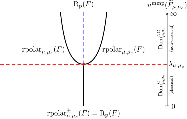
Figure 3.2: Pitchfork bifurcation diagram for $\operatorname{rpolar}_{\mu,\mu_{c}}^{\pm}(F)$ for $\mu>\mu_{c}\geq 0$. Let us express the energy-minimizers $\operatorname{rpolar}_{\mu,\mu_{c}}^{\pm}(F)$ in terms of the maximal mean planar stretch $u^{\rm mmp}(\widetilde{F}_{\mu,\mu_{c}})$ of the rescaled deformation gradient $\widetilde{F}_{\mu,\mu_{c}}\coloneqq\lambda_{\mu,\mu_{c}}^{-1}F$. For values $F\in\mathrm{Dom}^{\mathrm{C}}_{\mu,\mu_{c}}$, we have $0<u^{\rm mmp}\leq\lambda_{\mu,\mu_{c}}$ and the polar factor $\operatorname{R_{\rm p}}(F)$ is uniquely energy-minimizing. In contrast, for $F\in\mathrm{Dom}^{\mathrm{NC}}_{\mu,\mu_{c}}$, $\lambda_{\mu,\mu_{c}}\leq u^{\rm mmp}<\infty$, there are two non-classical minimizers $\operatorname{rpolar}^{\pm}_{\mu,\mu_{c}}(F)$. In this regime, the polar factor is no longer optimal but it is still a critical point. At the branching point $u^{\rm mmp}(\widetilde{F}_{\mu,\mu_{c}})=\lambda_{\mu,\mu_{c}}$ the minimizers all coincide: $\operatorname{rpolar}^{-}_{\mu,\mu_{c}}(F)=\operatorname{R_{\rm p}}(F)=\operatorname{rpolar}^{+}_{\mu,\mu_{c}}(F)$. For $\mu_{c}\to\mu$, the branching point escapes to infinity which asymptotically recovers the behavior in the classical parameter range $\mu_{c}\geq\mu>0$.

The domains of the piecewise definition of $\operatorname{rpolar}_{1,0}^{\pm}(F)$ in Corollary 3.6 indicate a certain tension-compression asymmetry in the material model characterized by the Cosserat shear–stretch energy $W_{1,0}(R\,;F)$; cf. Remark 3.15. We can also make a second important observation. To this end, consider a smooth curve $F(t):(-\varepsilon,\varepsilon)\to\operatorname{GL}^{+}(3)$. If the eigenvector $q_{3}(t)\in\mathbb{S}^{2}$ associated with the smallest singular value $\sigma_{3}(t)$ changes its orientation along this curve, then the rotation axis of $\operatorname{rpolar}_{1,0}^{\pm}(F)$ flips as well. Effectively, the sign of the relative rotation angle $\hat{\beta}_{1,0}^{\pm}(F)$ is negated which may lead to jumps. This can happen, e.g., if $F(t)$ passes through a deformation gradient with a non-simple singular value, but it may also depend on details of the specific algorithm used for the computation of the eigenbasis.

For the classical range $\mu_{c}\geq\mu>0$, the polar factor and the relaxed polar factor(s) coincide and trivially share all properties. This is no longer true for the non-classical parameter range $\mu_{c}\geq\mu>0$ and we compare the properties for that range in our next remark. More precisely, we present a detailed comparison of the well-known features of the polar factor $\operatorname{R_{\rm p}}$ which are of fundamental importance in the context of mechanics.

Remark 3.7 ($\operatorname{R_{\rm p}}(F)$ vs. $\operatorname{rpolar}(F)$ for the non-classical range $\mu>\mu_{c}\geq 0$).

Let $n\geq 2$ and $F\in\operatorname{GL}^{+}(n)$. The polar factor $\operatorname{R_{\rm p}}(F)\in\operatorname{SO}(n)$ obtained from the polar decomposition $F=\operatorname{R_{\rm p}}(F)\,U$ is always unique and satisfies:

$$\begin{matrix}[l]&\text{(Objectivity)}&\hskip 54.2025pt&\operatorname{R_{\rm p}}(\,Q\cdot F\,)&=&Q\cdot\operatorname{R_{\rm p}}(F)&\quad\quad(\forall Q\in\operatorname{SO}(n))\;,\\ &\text{(Isotropy)}&\hskip 54.2025pt&\operatorname{R_{\rm p}}(\,F\cdot Q\,)&=&\operatorname{R_{\rm p}}(F)\cdot Q&\quad\quad(\forall Q\in\operatorname{SO}(n))\;,\\ &\text{(Scaling invariance)}&\hskip 54.2025pt&\operatorname{R_{\rm p}}(\,\lambda\cdot F\,)&=&\operatorname{R_{\rm p}}(F)&\quad\quad(\forall\lambda>0)\;,\\ &\text{(Inversion symmetry)}&\hskip 54.2025pt&\operatorname{R_{\rm p}}(F^{-1})&=&\operatorname{R_{\rm p}}(F)^{-1}\;.&\end{matrix}$$ (3.12)

The relaxed polar factor(s) $\operatorname{rpolar}_{\mu,\mu_{c}}(F)\subset\operatorname{SO}(n)$ is in general multi-valued and, due to its variational characterization, satisfies:

$$\begin{matrix}[l]&\text{(Objectivity)}&\hskip 54.2025pt&\operatorname{rpolar}_{\mu,\mu_{c}}(\,Q\cdot F\,)&=&Q\cdot\operatorname{rpolar}_{\mu,\mu_{c}}(F)&\quad\quad(\forall Q\in\operatorname{SO}(n))\;,\\ &\text{(Isotropy)}&\hskip 54.2025pt&\operatorname{rpolar}_{\mu,\mu_{c}}(\,F\cdot Q\,)&=&\operatorname{rpolar}_{\mu,\mu_{c}}(F)\cdot Q&\quad\quad(\forall Q\in\operatorname{SO}(n))\;.\end{matrix}$$ (3.13)

For the particular dimensions $k=2,3$, our explicit formulae imply (cf. also Part I [29]) that there exist particular instances $\lambda^{*}>0$ and $F^{*}\in\operatorname{GL}^{+}(k)$ for which we have

$$\begin{matrix}[l]&\text{(\text@underline{Broken} scaling invariance)}&\hskip 54.2025pt&\operatorname{rpolar}^{\pm}_{\mu,\mu_{c}}(\lambda^{*}\cdot F^{*})&\neq&\operatorname{rpolar}(F^{*})&,\quad\text{and}\\ &\text{(\text@underline{Broken} inversion symmetry)}&\hskip 54.2025pt&\operatorname{rpolar}^{\pm}_{\mu,\mu_{c}}({F^{*}}^{-1})&\neq&\operatorname{rpolar}(F^{*})^{-1}&.\end{matrix}$$ (3.14)

This can be directly inferred from the partitioning of $\operatorname{GL}^{+}(k)=\mathrm{Dom}^{\mathrm{C}}_{\mu,\mu_{c}}\,\cup\,\mathrm{Dom}^{\mathrm{NC}}_{\mu,\mu_{c}}$ and the respective piecewise definition of the relaxed polar factor(s), see Corollary 3.6.

We interpret these broken symmetries as a (generalized) tension-compression asymmetry.

3.1 The reduced Cosserat shear–stretch energy

We now introduce the notion of a reduced energy which is realized by the energy-minimizing rotations $\operatorname{rpolar}_{\mu,\mu_{c}}(F)$; see also Remark 5.1.

Definition 3.8 (Reduced Cosserat shear–stretch energy).

The reduced Cosserat shear–stretch energy is defined as

$$W_{\mu,\mu_{c}}^{\rm red}:\operatorname{GL}^{+}(n)\to\operatorname{\sideset{}{{}_{0}^{+}}{\operatorname{\mathbb{R}}}},\quad\quad W_{\mu,\mu_{c}}^{\rm red}(F)\;\coloneqq\;\min_{R\,\in\,\operatorname{SO}(n)}\widehat{W}_{\mu,\mu_{c}}(R\,;F)\;.$$ (3.15)

Besides the previous definition, we also have the following equivalent means for the explicit computation of the reduced energy

$$W_{\mu,\mu_{c}}^{\rm red}(F) \;=\;\widehat{W}_{\mu,\mu_{c}}(\operatorname{rpolar}^{\pm}_{\mu,\mu_{c}}(F)\,;F)\;,\quad\text{and}$$ (3.16)

$$W_{\mu,\mu_{c}}^{\rm red}(F) \;=\;\widehat{W}_{\mu,\mu_{c}}^{\rm red}(D)\;\coloneqq\min_{\widehat{R}\in\operatorname{SO}(n)}\widehat{W}_{\mu,\mu_{c}}(\widehat{R}\,;D)\;=\;\widehat{W}_{\mu,\mu_{c}}(\widehat{R}_{\mu,\mu_{c}}^{\pm}\,;D)\;.$$

We now approach the computation of the explicit representation of $W_{\mu,\mu_{c}}^{\rm red}(F)$ by means of the equivalent expression $\widehat{W}^{\rm red}_{\mu,\mu_{c}}(D)$. For the sake of brevity, we set $c=\frac{2}{\sigma_{1}+\sigma_{2}}=1/u^{\rm mmp}(F)$ and $s=\sqrt{1-c^{2}}$. This allows us to write the optimal relative Cosserat rotations in a simple form in the computation of

$$\widehat{R}_{1,0}^{\pm}D=\begin{pmatrix}c&\mp s&0\\ \pm s&c&0\\ 0&0&1\\ \end{pmatrix}\begin{pmatrix}\sigma_{1}&0&0\\ 0&\sigma_{2}&0\\ 0&0&\sigma_{3}\end{pmatrix}=\begin{pmatrix}\sigma_{1}\cdot c&\mp\sigma_{2}\cdot s&0\\ \pm\sigma_{1}\cdot s&\sigma_{2}\cdot c&0\\ 0&0&\sigma_{3}\\ \end{pmatrix}\;.$$ (3.17)

From this, we compute the following symmetric and skew-symmetric parts:

$$\operatorname{sym}\left(\widehat{R}_{1,0}^{\pm}D-{\boldsymbol{\mathbbm{1}}}\right)\,\;=\;\begin{pmatrix}\sigma_{1}\cdot c-1&\frac{d_{12}}{2}\cdot s&0\\ \frac{d_{12}}{2}\cdot s&\sigma_{2}\cdot c-1&0\\ 0&0&\sigma_{3}-1\\ \end{pmatrix}\;,\quad\text{and}$$ (3.18)

$$\operatorname{skew}\left(\widehat{R}_{1,0}^{\pm}D-{\boldsymbol{\mathbbm{1}}}\right)\;=\;{\begin{pmatrix}0&\mp\frac{s_{12}}{2}\cdot s&\hskip 5.69046pt0\\ \pm\frac{s_{12}}{2}\cdot s&0&\hskip 5.69046pt0\\ 0&0&\hskip 5.69046pt0\\ \end{pmatrix}}\;.$$

Lemma 3.9 (The reduced Cosserat shear–stretch energy $\operatorname{W^{\rm red}_{1,0}}(F)$ in terms of singular values).

Let $F\in\operatorname{GL}^{+}(3)$ and $\sigma_{1}>\sigma_{2}>\sigma_{3}>0$ the ordered singular values of $F$. Then the reduced Cosserat shear–stretch energy $\operatorname{W^{\rm red}_{1,0}}(F)$ admits the following piecewise representation

$$\operatorname{W^{\rm red}_{1,0}}(F)\,=\,\begin{cases}\,(\sigma_{1}-1)^{2}+(\sigma_{2}-1)^{2}+(\sigma_{3}-1)^{2}=\left\lVert U-{\boldsymbol{\mathbbm{1}}}\right\rVert^{2}&,\,\text{if}\;\,\sigma_{1}+\sigma_{2}\leq 2,\,\text{i.e.},\,F\in\mathrm{Dom}^{\mathrm{C}}_{1,0}\,,\\ \,\frac{1}{2}\,(\sigma_{1}-\sigma_{2})^{2}+(\sigma_{3}-1)^{2}&,\,\text{if}\;\,\sigma_{1}+\sigma_{2}\geq 2,\,\text{i.e.},\,F\in\mathrm{Dom}^{\mathrm{NC}}_{1,0}\,.\\ \end{cases}$$

Proof. The classical piece of the energy is easily obtained by inserting the polar factor $\operatorname{R_{\rm p}}(F)$ into the energy. To compute the non-classical piece, we first recall that

$$\left\lVert\operatorname{sym}(\operatorname{rpolar}^{\pm}(F)^{T}F-{\boldsymbol{\mathbbm{1}}})\right\rVert^{2}\;=\;\operatorname{W^{\rm red}_{1,0}}(F)\;=\;\widehat{W}^{\rm red}_{1,0}(D)\;=\;\left\lVert\operatorname{sym}(\widehat{R}^{\pm}D-{\boldsymbol{\mathbbm{1}}})\right\rVert^{2}\;.$$

We compute the expression on the right hand side. To this end, we set $c=\frac{2}{\sigma_{1}+\sigma_{2}}$ and $s=\sqrt{1-c^{2}}$ again and compute the Frobenius matrix norm of $\operatorname{sym}(\widehat{R}^{\pm}D-1)$ which we have derived in (3.18). This gives us

$$\left\lVert\operatorname{sym}\left(\widehat{R}^{\pm}D-{\boldsymbol{\mathbbm{1}}}\right)\right\rVert^{2} =(\sigma_{1}c-1)^{2}+(\sigma_{2}c-1)^{2}+\frac{1}{2}\,(\sigma_{1}-\sigma_{2})^{2}(1-c^{2})+(\sigma_{3}-1)^{2}$$

$$=\frac{1}{2}\left(4+(\sigma_{1}-\sigma_{2})^{2}-4c(\sigma_{1}+\sigma_{2})+c^{2}(\sigma_{1}+\sigma_{2})^{2}\right)+(\sigma_{3}-1)^{2}$$

$$=\frac{1}{2}(\sigma_{1}-\sigma_{2})^{2}+(\sigma_{3}-1)^{2}\;. \blacksquare$$

Our next step is to reveal the form of the reduced energy for the entire non-classical parameter range $\mu>\mu_{c}\geq 0$ which involves the parameter reduction lemma, but we have to be a bit careful.

Remark 3.10 (Reduced energies and the parameter reduction lemma).

The parameter reduction procedure described in [29, Lem. 2.2] is the key to the minimizers for general non-classical material parameters $\mu>\mu_{c}\geq 0$. It might be tempting, but we have to stress that the general form of the reduced energy cannot be obtained by rescaling the singular values $\sigma_{i}\mapsto\lambda_{\mu,\mu_{c}}^{-1}\sigma_{i}$ in the singular value representation of $W^{\rm red}_{1,0}$.

Theorem 3.11 ($W^{\rm red}_{\mu,\mu_{c}}$ as a function of the singular values).

Let $F\in\operatorname{GL}^{+}(n)$ and $\sigma_{1}>\sigma_{2}>\sigma_{3}>0$, the ordered singular values of $F$ and let $\mu>\mu_{c}\geq 0$, i.e., a non-classical parameter set. Then the reduced Cosserat shear–stretch energy $W^{\rm red}_{\mu,\mu_{c}}:\operatorname{GL}^{+}(3)\to\operatorname{\sideset{}{{}_{0}^{+}}{\operatorname{\mathbb{R}}}}$ admits the following explicit representation

$$W^{\rm red}_{\mu,\mu_{c}}(F)\,=\,\begin{cases}\,\mu\left((\sigma_{1}-1)^{2}+(\sigma_{2}-1)^{2}+(\sigma_{3}-1)^{2}\right)=\mu\,\left\lVert U-{\boldsymbol{\mathbbm{1}}}\right\rVert^{2}&,\;F\in\mathrm{Dom}^{\mathrm{C}}_{\mu,\mu_{c}}\;,\\ \,\frac{\mu}{2}(\sigma_{1}-\sigma_{2})^{2}+\mu\,(\sigma_{3}-1)^{2}+\frac{\mu_{c}}{2}\left(\left(\sigma_{1}+\sigma_{2}\right)-\operatorname{\rho_{\mu,\,\mu_{c}}}\right)^{2}-\frac{\mu_{c}}{2}\cdot\rho_{\mu,\mu_{c}}^{2}&,\;F\in\mathrm{Dom}^{\mathrm{NC}}_{\mu,\mu_{c}}\;.\end{cases}$$

Proof. In order to obtain the classical part of the energy it suffices to insert $\operatorname{R_{\rm p}}{}$ into the energy. For the non-classical piece, we insert the optimal relative rotations $\widehat{R}_{\mu,\mu_{c}}^{\pm}$ into $\widehat{W}_{\mu,\mu_{c}}(\widehat{R}\,;D)$. This amounts to replace $c\mapsto\tilde{c}=\frac{\operatorname{\rho_{\mu,\,\mu_{c}}}}{\sigma_{1}+\sigma_{2}}$ and $s\mapsto\tilde{s}=\sqrt{1-\tilde{c}^{2}}$ in our preparatory calculation (3.18). This yields the following contributions:

$$\mu\;\left\lVert\operatorname{sym}(\widehat{R}_{\mu,\mu_{c}}^{\pm}D-{\boldsymbol{\mathbbm{1}}})\right\rVert^{2} \;=\;\frac{\mu}{2}\;d_{12}^{2}+\mu\,(\sigma_{3}-1)^{2}+\frac{\mu}{2}(\operatorname{\rho_{\mu,\,\mu_{c}}}-\,2)^{2}\;,$$ (3.19)

$$\mu_{c}\;\left\lVert\operatorname{skew}(\widehat{R}_{\mu,\mu_{c}}^{\pm}D-{\boldsymbol{\mathbbm{1}}})\right\rVert^{2} \;=\;\frac{\mu_{c}}{2}\;s_{12}^{2}\;\tilde{s}^{2}\;=\;\frac{\mu_{c}}{2}s_{12}^{2}-\frac{\mu_{c}}{2}\operatorname{\rho_{\mu,\,\mu_{c}}}^{2}\;.$$ (3.20)

Finally, adding only the constant part of the symmetric contribution to the complete contribution due to the skew-symmetric part, we obtain

$$\frac{\mu}{2}(\operatorname{\rho_{\mu,\,\mu_{c}}}-2)^{2}+\frac{\mu_{c}}{2}s_{12}^{2}-\frac{\mu_{c}}{2}\operatorname{\rho_{\mu,\,\mu_{c}}}^{2}=\frac{\mu_{c}}{2}\left(s^{2}_{12}-2\operatorname{\rho_{\mu,\,\mu_{c}}}\right)=\frac{\mu_{c}}{2}\left(s_{12}-\operatorname{\rho_{\mu,\,\mu_{c}}}\right)^{2}-\frac{\mu_{c}}{2}\;\rho_{\mu,\mu_{c}}^{2}\;. \blacksquare$$

The last step of the preceding proof is interesting in its own right.

Remark 3.12 (On $\mu_{c}$ as a penalty weight).

Let us consider the contribution of the skew-term to $W^{\rm red}_{\mu,\mu_{c}}$ given by μc2((σ_1 + σ_2) - ρ_μ, μ_c)^2 as a penalty term for $F\in\operatorname{GL}^{+}(3)$ arising for material parameters in the non-classical parameter range $\mu>\mu_{c}\geq 0$. This leads to a simple but interesting observation for strictly positive $\mu_{c}>0$. The minimizers $F\in\operatorname{GL}^{+}(3)$ for the penalty term satisfy the bifurcation criterion σ_1 + σ_2 = ρ_μ, μ_c for $\operatorname{rpolar}^{\pm}_{\mu,\mu_{c}}(F)$. In this case $\widehat{R}_{\mu,\mu_{c}}^{\pm}={\boldsymbol{\mathbbm{1}}}$ which implies that $\widehat{R}_{\mu,\mu_{c}}^{\pm}D-{\boldsymbol{\mathbbm{1}}}\in{\rm{Sym}}(3)$, i.e., it is symmetric. Hence, the skew-part vanishes entirely which minimizes the penalty. In numerical applications, a rotation field $R$ approximating $\operatorname{rpolar}^{\pm}(F)$ can be expected to be unstable in the vicinity of the branching point $\sigma_{1}+\sigma_{2}\approx\operatorname{\rho_{\mu,\,\mu_{c}}}$. Hence, a penalty which explicitly rewards an approximation to the bifurcation point seems to be a delicate property. In strong contrast, for the case when the Cosserat couple modulus is zero, i.e., $\mu_{c}=0$, the penalty term vanishes entirely. This hints at a possibly more favorable qualitative behavior of the model in that case; cf. [60].

3.2 Geometric aspects of the reduced Cosserat shear–stretch energy

We recall that the tangent bundle $T\operatorname{SO}(n)$ is isomorphic to the product $\operatorname{SO}(n)\times\operatorname{\mathfrak{so}}(n)$ as a vector bundle. This is commonly referred to as the left trivialization, see, e.g., [24]. With this we can comfortably minimize over the tangent bundle in the following lemma which sets the course for our next theorem.

Lemma 3.13.

Let $F\in\operatorname{\mathbb{R}}^{n\times n}$. Then

$$\inf_{\begin{subarray}{c}R\,\in\,\operatorname{SO}(3)\\ A\,\in\,\operatorname{\mathfrak{so}}(3)\end{subarray}}\|R^{T}F-{\boldsymbol{\mathbbm{1}}}-A\|^{2}\quad=\quad\min_{R\,\in\,\operatorname{SO}(3)}\|\operatorname{sym}(R^{T}F-{\boldsymbol{\mathbbm{1}}})\|^{2}\quad\eqqcolon\quad\min_{R\,\in\,\operatorname{SO}(3)}W_{1,0}(R\,;F)\;.$$

Proof.

For all $R\,\in\,\operatorname{SO}(3)$, the infimum of $\left\lVert\operatorname{skew}(R^{T}F-{\boldsymbol{\mathbbm{1}}})-A\right\rVert^{2}$ over all skew symmetric $A$ is obviously attained at $A=\operatorname{skew}(R^{T}F-{\boldsymbol{\mathbbm{1}}})$. Therefore

$$\smash{\inf_{{\begin{subarray}{c}R\,\in\,\operatorname{SO}(3)\\ A\,\in\,\operatorname{\mathfrak{so}}(3)\end{subarray}}}}\,\left\lVert R^{T}F-{\boldsymbol{\mathbbm{1}}}-A\right\rVert^{2} =\inf_{R\,\in\,\operatorname{SO}(3)}\,\inf_{A\,\in\,\operatorname{\mathfrak{so}}(3)}\Big{\{}\left\lVert\operatorname{sym}(R^{T}F-{\boldsymbol{\mathbbm{1}}}-A)\right\rVert^{2}+\left\lVert\operatorname{skew}(R^{T}F-{\boldsymbol{\mathbbm{1}}}-A)\right\rVert^{2}\Big{\}}$$

$$=\inf_{R\,\in\,\operatorname{SO}(3)}\,\Big{\{}\left\lVert\operatorname{sym}(R^{T}F-{\boldsymbol{\mathbbm{1}}})\right\rVert^{2}+\inf_{A\,\in\,\operatorname{\mathfrak{so}}(3)}\left\lVert\operatorname{skew}(R^{T}F-{\boldsymbol{\mathbbm{1}}})-A\right\rVert^{2}\Big{\}}$$

$$=\inf_{R\,\in\,\operatorname{SO}(3)}\,\left\lVert\operatorname{sym}(R^{T}F-{\boldsymbol{\mathbbm{1}}})\right\rVert^{2}\;.$$

Since $\operatorname{SO}(3)$ is compact and $W_{1,0}(R\,;F)$ is continuous, the infimum is attained by a minimizer. $\blacksquare$

The preceding lemma leads us to a nice geometric characterization of the reduced Cosserat shear–stretch energy which we find quite remarkable. It might even be useful for the case $n\geq 4$ although this is somewhat far-fetched.

Corollary 3.14 (Characterization of $W_{1,0}^{\rm red}$ as a distance).

Let $n\geq 2$ and consider $F\in\operatorname{GL}^{+}(n)$ with singular values $\sigma_{1}\geq\sigma_{2}\geq\ldots\geq\sigma_{n}>0$ not necessarily distinct. Then the reduced Cosserat shear–stretch energy $W_{1,0}^{\rm red}:\operatorname{GL}^{+}(n)\to\operatorname{\sideset{}{{}_{0}^{+}}{\operatorname{\mathbb{R}}}}$ admits the following characterization as a distance:

$$W^{\rm red}(F)\quad=\quad\operatorname{dist}_{\rm euclid}^{2}\big{(}F,\,\operatorname{SO}(n)\left({\boldsymbol{\mathbbm{1}}}+\operatorname{\mathfrak{so}}(n)\right)\big{)}\;.$$ (3.21)

Here, $\operatorname{dist}_{\rm euclid}$ denotes the euclidean distance function.

Proof. First note that

$$W^{\rm red}_{1,0}(F) \coloneqq\min_{R\,\in\,\operatorname{SO}(n)}\|\operatorname{sym}(R^{T}F-{\boldsymbol{\mathbbm{1}}})\|^{2}\stackrel{{\scriptstyle(\text{Lem. \ref{lem:dist_ctb_technical}})}}{{=}}\smash{\inf_{\begin{subarray}{c}R\,\in\,\operatorname{SO}(3)\\ A\,\in\,\operatorname{\mathfrak{so}}(3)\end{subarray}}}\|R^{T}F-{\boldsymbol{\mathbbm{1}}}-A\|^{2}$$

$$=\inf_{\begin{subarray}{c}R\,\in\,\operatorname{SO}(3)\\ A\,\in\,\operatorname{\mathfrak{so}}(3)\end{subarray}}\|R(R^{T}F-{\boldsymbol{\mathbbm{1}}}-A)\|^{2}\;.$$

The last step ist justified by the orthogonal invariance of the Frobenius norm $\|\cdot\|$. Carrying out the multiplications on the right hand side, we are lead to the conclusion

$$\inf_{\begin{subarray}{c}R\,\in\,\operatorname{SO}(3)\\ A\,\in\,\operatorname{\mathfrak{so}}(3)\end{subarray}}\|F-R\,{\boldsymbol{\mathbbm{1}}}-RA\|^{2}=\inf_{\begin{subarray}{c}R\,\in\,\operatorname{SO}(3)\\ A\,\in\,\operatorname{\mathfrak{so}}(3)\end{subarray}}\|F-R({\boldsymbol{\mathbbm{1}}}+A)\|^{2}\eqqcolon\operatorname{dist}_{\rm euclid}^{2}(F,\operatorname{SO}(n)\left({\boldsymbol{\mathbbm{1}}}+\operatorname{\mathfrak{so}}(n)\right))\;. \blacksquare$$

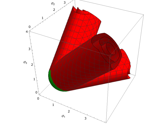
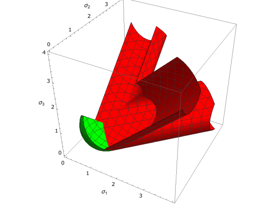
Figure 3.3: Energy isosurfaces of $W^{\rm red}_{1,0}$ considered as a function of the unordered singular values $\sigma_{1},\sigma_{2},\sigma_{3}>0$ of $F\in\operatorname{GL}^{+}(3)$. The displayed contour levels are $0.1$, $0.4$ and $0.8$. On the right, we have removed a piece from the non-classical cylindrical parts (red) of the energy level $0.8$ which reveals the spherical shell of the classical part (green). Note that a computation of these level surfaces via Monte Carlo minimization yields the same result (but at a much lower resolution).

Remark 3.15 (Zero reduced energy and tension-compression asymmetry).

A sharp look at Lemma 3.9 is sufficient to see that the $0$-energy level of $W^{\rm red}_{1,0}$ precisely corresponds to singular value tuples of the form $(s,s,1)$, $s\in[1,\infty)$. In our Figure 3.3 tuples of this type (and permutations thereof) correspond to the axes of the cylindrical sheets of the isosurfaces. Let us now consider $X=R({\boldsymbol{\mathbbm{1}}}+A)$, $R\in\operatorname{SO}(3)$, $A\in\operatorname{\mathfrak{so}}(3)$, which has the squared singular values $(\sigma_{1}^{2},\sigma_{2}^{2},\sigma_{3}^{2})=\left(1+\left\lVert A\right\rVert^{2},1+\left\lVert A\right\rVert^{2},1\right)$. Clearly, such a matrix $X$ does not generate any reduced Cosserat shear–stretch energy at all – in perfect accord with Corollary 3.14. Geometrically, $U(X)\coloneqq\sqrt{X^{T}X}$ induces a homogeneous blow-up (i.e., a rescaling of arbitrary positive magnitude) of the plane of maximal strain $\mathrm{P}^{\rm mp}(X)$ while preserving the distance of any given point to this plane. Furthermore, there is no possibility of similar energy savings in the compressive range for $F\in\operatorname{GL}^{+}(3)$ where the classical piece of $W^{\rm red}_{1,0}$ is active. It seems to us that this makes a good case for a quite remarkable type of tension-compression asymmetry.

3.3 Alternative criteria for the existence of non-classical solutions

For $\mu>\mu_{c}>0$, i.e., for strictly positive $\mu_{c}>0$, the singular radius satisfies $\operatorname{\rho_{\mu,\,\mu_{c}}}\coloneqq\frac{2\mu}{\mu-\mu_{c}}>2$. We now define a quite similar constant, namely

$$\zeta_{\mu,\mu_{c}}\coloneqq\operatorname{\rho_{\mu,\,\mu_{c}}}-\;\rho_{1,0}=\frac{2\mu_{c}}{\mu-\mu_{c}}>0\;.$$ (3.22)

Furthermore, we define the $\varepsilon$-neighborhood of a set $\mathcal{X}\subseteq\operatorname{\mathbb{R}}^{n\times n}$ relative to the euclidean distance function as N_ε(X)  ≔  {Y ∈R^n ×n  —  dist_euclid(Y, X) ¡ ε} .

Figure 3.4: Illustration of a euclidean $\varepsilon$-neighborhood of $\operatorname{SO}(3)\subset\operatorname{\mathbb{R}}^{3\times 3}$.

Lemma 3.16 (Classical $\operatorname{SO}(3)$-neighborhood for $\mu_{c}>0$).

Let $\mu>\mu_{c}>0$, $F\in\operatorname{GL}^{+}(3)$ and $\zeta_{\mu,\mu_{c}}\coloneqq\frac{2\mu_{c}}{\mu-\mu_{c}}>0$. Then we have the following inclusion

$$N_{\frac{1}{2}\zeta_{\mu,\mu_{c}}^{2}}(\operatorname{SO}(3))\quad\subset\quad\mathrm{Dom}^{\mathrm{C}}_{\mu,\mu_{c}}\;.$$ (3.23)

In other words, for all $F\in\operatorname{GL}^{+}(3)$ satisfying $\operatorname{dist}_{\rm euclid}(F,\operatorname{SO}(3))=\left\lVert U-{\boldsymbol{\mathbbm{1}}}\right\rVert^{2}<\frac{1}{2}\zeta_{\mu,\mu_{c}}^{2}$, the polar factor $\operatorname{R_{\rm p}}{}$ is the unique minimizer of $W_{\mu,\mu_{c}}(R\,;F)$.

Proof.

Since $\operatorname{dist}_{\rm euclid}^{2}(F,\operatorname{SO}(3))=\|U-{\boldsymbol{\mathbbm{1}}}\|^{2}=\sum_{i=1}^{3}(\sigma_{i}-1)^{2}$ by Grioli’s theorem [69], we find

$$\operatorname{dist}_{\rm euclid}^{2}(F,\operatorname{SO}(3))<\frac{1}{2}\;\zeta_{\mu,\mu_{c}}^{2}\quad\Longrightarrow \quad 2\left((\sigma_{1}-1)^{2}+(\sigma_{2}-1)^{2}+(\sigma_{3}-1)^{2}\right)<\zeta_{\mu,\mu_{c}}^{2}$$

$$\quad\Longrightarrow \quad 2\left((\sigma_{1}-1)^{2}+(\sigma_{2}-1)^{2}\right)<\zeta_{\mu,\mu_{c}}^{2}\;.$$

Further, $0\leq(a-b)^{2}=a^{2}+b^{2}-2ab$ implies $2\,(a^{2}+b^{2})\geq a^{2}+b^{2}+2ab$ and it follows that

$$(\sigma_{1}-1)^{2}+(\sigma_{2}-1)^{2}+2(\sigma_{1}-1)(\sigma_{2}-1)<\zeta_{\mu,\mu_{c}}^{2}\;.$$ (3.24)

Completing the square and taking square roots on both sides, we find

$$\left((\sigma_{1}-1)+(\sigma_{2}-1)\right)^{2}<\zeta^{2}_{\mu,\mu_{c}}\quad\Longrightarrow\quad\pm\left|(\sigma_{1}-1)+(\sigma_{2}-1)\right|<\zeta_{\mu,\mu_{c}}\;.$$ (3.25)

Inserting $\zeta_{\mu,\mu_{c}}\coloneqq\operatorname{\rho_{\mu,\,\mu_{c}}}-\;2$, we obtain $(\sigma_{1}-1)+(\sigma_{2}-1)\;<\;\rho_{\mu_{,}\mu_{c}}-\;2$. This implies $\sigma_{1}+\sigma_{2}<\rho_{\mu_{,}\mu_{c}}$ and hence $F\in\mathrm{Dom}^{\mathrm{C}}_{\mu,\mu_{c}}$. $\blacksquare$

Note that the preceding proof can be quite easily adapted to the planar case $n=2$ presented in [29].

Lemma 3.17.

Let $F\in\operatorname{SL}(3)$, i.e., ${\operatorname{det}[{F}]}=\sigma_{1}\sigma_{2}\sigma_{3}=1$, where $\sigma_{1}\geq\sigma_{2}\geq\sigma_{3}>0$ are ordered singular values of $F$, not necessarily distinct. Then

$$\operatorname{SL}(3)\quad\subset\quad\mathrm{Dom}^{\mathrm{NC}}_{1,0}\;,$$ (3.26)

i.e., $F$ induces a strictly non-classical minimizer. Equivalently, ${\operatorname{det}[{F}]}=1$ implies the estimate $\sigma_{1}+\sigma_{2}\geq 2$.

Proof.

The inequality for the geometric and arithmetic mean shows that

$$\frac{\sigma_{1}+\sigma_{2}+\sigma_{3}}{3}\quad\geq\quad(\sigma_{1}\,\sigma_{2}\,\sigma_{3})^{\frac{1}{3}}\quad=\quad 1\;.$$ (3.27)

It follows that $\sigma_{1}+\sigma_{2}\geq 3-\sigma_{3}$ which implies the claim for $\sigma_{3}\leq 1$. Due to the ordering $\sigma_{1}\geq\sigma_{2}\geq\sigma_{3}>0$, the case $\sigma_{3}>1$ contradicts our assumption ${\operatorname{det}[{F}]}>1$. $\blacksquare$

Remark 3.18.

If we make the stronger assumption $\sigma_{1}>\sigma_{2}>\sigma_{3}>0$, we obtain a strict inequality $\sigma_{1}+\sigma_{2}>2$. In that case, $F\in\mathrm{Dom}^{\mathrm{NC}}_{1,0}\setminus\mathrm{Dom}^{\mathrm{C}}_{1,0}$ is strictly non-classical.

Corollary 3.19.

Let $\mu>0$, $F\in\operatorname{SL}^{+}(3)$ and assume that $\sigma_{1}>\sigma_{2}>\sigma_{3}>0$. Then

$$F\quad\in\quad\mathrm{Dom}^{\mathrm{NC}}_{\mu,0}\setminus\mathrm{Dom}^{\mathrm{C}}_{\mu,0}\;,$$ (3.28)

i.e., the minimizers $\operatorname{rpolar}_{\mu,0}^{\pm}(F)\neq\operatorname{R_{\rm p}}{}$ are strictly non-classical.

Proof.

Since $\lambda_{\mu,0}=1$, it follows that $\widetilde{F}_{\mu,0}=F$. Further $\rho_{\mu,0}=\rho_{1,0}$. Thus, we are in the hypotheses of the preceding Lemma 3.17 for the case where the inequality is strict, see Remark 3.18. $\blacksquare$

3.4 Application

Let us now give a short application to our previous findings. We consider a so-called volumetric-isochoric split for the geometrically nonlinear Cosserat shear–stretch energy. Note that this material model appears in a variety of contexts, see, e.g., [26, 9, 63, 45, 58, 57, 62, 31, 78, 80], and, recently [84, 51, 6, 7]. Further, similar expressions for the strain energy have been considered in the context of plate and shell theories, see, e.g., [74, 27, 75, 59, 4, 5, 77].

Let us introduce the isochoric projection $F\mapsto F_{\rm iso}\coloneqq\frac{F}{{\operatorname{det}[{F}]}^{1/3}}\in\operatorname{SL}(3)$ of the deformation gradient $F\in\operatorname{GL}^{+}(3)$ which can also be applied to $\overline{U}\coloneqq R^{T}F$. With this notation, we obtain

$$W(\overline{U}) =\underbrace{\mu\,\left\lVert\operatorname{sym}\left(\frac{\overline{U}}{{\operatorname{det}[{\overline{U}}]}^{1/3}}-{\boldsymbol{\mathbbm{1}}}\right)\right\rVert^{2}\;+\;\mu_{c}\,\left\lVert\operatorname{skew}\left(\frac{\overline{U}}{{\operatorname{det}[{\overline{U}}]}^{1/3}}-{\boldsymbol{\mathbbm{1}}}\right)\right\rVert^{2}}_{\text{``Cosserat shear--stretch energy''}}\;+\;\underbrace{\vphantom{\left\lVert\operatorname{sym}\left(\frac{\overline{U}}{{\operatorname{det}[{\overline{U}}]}^{1/3}}-{\boldsymbol{\mathbbm{1}}}\right)\right\rVert^{2}}h({\operatorname{det}[{\overline{U}}]})}_{\text{``volumetric contribution''}}$$

$$=\mu\,\left\lVert\operatorname{sym}\left(R^{T}\frac{F}{{\operatorname{det}[{F}]}^{1/3}}-{\boldsymbol{\mathbbm{1}}}\right)\right\rVert^{2}\;+\;\mu_{c}\,\left\lVert\operatorname{skew}\left(R^{T}\frac{F}{{\operatorname{det}[{F}]}^{1/3}}-{\boldsymbol{\mathbbm{1}}}\right)\right\rVert^{2}\;+\;h({\operatorname{det}[{R^{T}F}]})$$

$$=\mu\,\left\lVert\operatorname{sym}\left(R^{T}F_{\rm iso}-{\boldsymbol{\mathbbm{1}}}\right)\right\rVert^{2}\;+\;\mu_{c}\,\left\lVert\operatorname{skew}\left(R^{T}F_{\rm iso}-{\boldsymbol{\mathbbm{1}}}\right)\right\rVert^{2}\;+\;h({\operatorname{det}[{F}]})\;.$$

The results of the previous subsections, allow us to determine the optimal Cosserat rotations for the split energy $W(\overline{U})\;=\;W(R^{T}F)\;=\;\operatorname{W_{\mu,\mu_{c}}}(R\,;F_{\rm iso})\;+\;h({\operatorname{det}[{F}]})$. Note first that the additional volumetric contribution $h({\operatorname{det}[{F}]})$ penalizes volume change by a scalar function $h:\operatorname{\operatorname{\mathbb{R}}^{+}}\to\operatorname{\sideset{}{{}_{0}^{+}}{\operatorname{\mathbb{R}}}}$ which is constant with respect to $R\in\operatorname{SO}(3)$. Therefore, this formulation still gives rise to the same optimal Cosserat rotations rpolar_μ,μ_c(F_iso) ≔ =  .

We can now make an interesting observation. To this end, let $\varepsilon>0$ and consider diagonal matrices of the type

$$D_{\varepsilon}\;\coloneqq\;\begin{pmatrix}\operatorname{\rho_{\mu,\,\mu_{c}}}-\,1+\varepsilon&0&0\\ 0&1&0\\ 0&0&(\operatorname{\rho_{\mu,\,\mu_{c}}}-\,1+\varepsilon)^{-1}\end{pmatrix}\;\in\;\operatorname{SL}(3)\;.$$

The required ordering $\sigma_{1}>\sigma_{2}>\sigma_{3}>0$ follows from $\operatorname{\rho_{\mu,\,\mu_{c}}}\coloneqq\frac{2\mu}{\mu-\mu_{c}}\geq\frac{2\mu}{\mu}=2$ and holds for the entire non-classical parameter range $\mu>\mu_{c}\geq 0$. Obviously, we have

$$\sigma_{1}+\sigma_{2}=\operatorname{\rho_{\mu,\,\mu_{c}}}+\;\varepsilon>\operatorname{\rho_{\mu,\,\mu_{c}}}\quad\Longrightarrow\quad D_{\varepsilon}\in\mathrm{Dom}^{\mathrm{NC}}_{\mu,\mu_{c}}\setminus\mathrm{Dom}^{\mathrm{C}}_{\mu,\mu_{c}}\;.$$

Hence, the intersection $\operatorname{SL}(3)\cap\left(\mathrm{Dom}^{\mathrm{NC}}_{\mu,\mu_{c}}\setminus\mathrm{Dom}^{\mathrm{C}}_{\mu,\mu_{c}}\right)\neq\emptyset$ is never empty since it contains $D_{\varepsilon}$ for all $\varepsilon>0$. Furthermore, the associated optimal Cosserat rotations are strictly non-classical, i.e., $\operatorname{rpolar}^{\pm}_{\mu,\mu_{c}}(D_{\varepsilon})\neq\operatorname{R_{\rm p}}(D_{\varepsilon})={\boldsymbol{\mathbbm{1}}}$.

Hence, in order to assure that there can be no strictly non-classical optimal Cosserat rotations (for whatever reason) one has to consider material parameters from the classical parameter range $\mu_{c}\geq\mu>0$. In this case the Cosserat couple modulus $\mu_{c}$ dominates the Lamé shear modulus $\mu$ and Grioli’s theorem assures that the polar factor $\operatorname{R_{\rm p}}(F)$ is always uniquely optimal [69].

In the distinguished limit case $\mu_{c}=0$, the volumetric-isochoric split precludes the previously observed tension-compression asymmetry. In this particular scenario, Corollary 3.19 shows that the optimal rotations are always non-classical. Since no bifurcation of the optimal rotations occurs, there can be no qualitatively different energetic response under tension and compression for $\mu_{c}=0$; cf. also [60] for a discussion of other implications of a zero Cosserat couple modulus.

Last but not least, we want to mention that our proposed explicit formulae for optimal Cosserat rotations may also lead to improved stability and performance in full scale 3D nonlinear finite element computations for media with rotational microstructure. We expect them to be especially useful for the highly interesting and numerically challenging case of a material with small internal length scale $L_{\rm c}>0$. If, in addition, the volumetric contribution is independent of the rotation (see above), then the optimal Cosserat rotations $\operatorname{rpolar}^{\pm}_{\mu,\mu_{c}}(F)$ proposed in Corollary 3.6 can be expected to be ideal candidates for the initialization of the Newton–iterations for the field of microrotations $R:\Omega\subset\operatorname{\mathbb{R}}^{n}\to\operatorname{SO}(n)$, $n=2,3$.

4 Dissection of critical point structure and computational validation of optimality

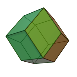
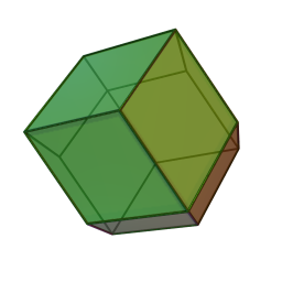
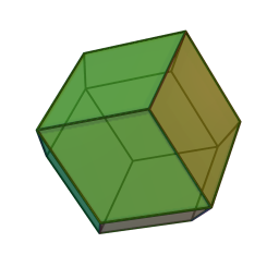
Figure 4.1: A rhombic dodecahedron placed in the space of unordered singular values $(\sigma_{1},\sigma_{2},\sigma_{3})\in\operatorname{\mathbb{R}}^{3}$ of $F\in\operatorname{GL}^{+}(3)$ gives rise to a beautiful geometric characterization of the classical and non-classical domains $\mathrm{Dom}^{\mathrm{C}}_{1,0}$ and $\mathrm{Dom}^{\mathrm{NC}}_{1,0}$. Pick a face and displace it in normal direction while scaling it by its distance to the origin. This creates a convex cone with the scaled faces as cross-sections which intersects the polytope. The part of the cone inside the polytope corresponds to singular values $(\sigma_{1},\sigma_{2},\sigma_{3})\in\operatorname{\mathbb{R}}^{3}$ in $\mathrm{Dom}^{\mathrm{C}}_{1,0}$. The exterior part corresponds to $\mathrm{Dom}^{\mathrm{NC}}_{1,0}$. On the picked face itself $\mathrm{Dom}^{\mathrm{C}}_{1,0}\cap\mathrm{Dom}^{\mathrm{NC}}_{1,0}$, the two branches coincide. (This is how we discovered the non-classical bifurcation behavior of $\operatorname{rpolar}^{\pm}_{1,0}(F)$ in dimension $n\!=\!3$.)

We recall that our primary objective for the present work is to derive a formula (or algorithm) which allows to compute the set of optimal Cosserat rotations $\operatorname{rpolar}_{\mu,\mu_{c}}(F)\subset\operatorname{SO}(3)$, i.e., the rotations which minimize the Cosserat shear–stretch energy $\operatorname{W_{\mu,\mu_{c}}}(R\,;F)$ for given $F\in\operatorname{GL}^{+}(3)$ and weights $(\mu,\mu_{c})$ in the non-classical parameter range $\mu>\mu_{c}\geq 0$. In the first two sections of this contribution, we have hopefully convinced our avid reader that it suffices to solve Problem 1.5 in order to determine the optimal Cosserat rotations which then solve our original Problem 1.1. However, in order to simultaneously cross-validate our theoretical derivation (this includes the parameter reduction presented in Part I [29, Lem. 2.2, p. 4]), we have based our final validation on Problem 1.1. This bypasses all simplification steps which we have used in order to derive the formula for $\operatorname{rpolar}_{\mu,\mu_{c}}^{\pm}(F)$ proposed in Corollary 3.6, but is costly due to the large parameter space.

4.1 Interactive analysis of the critical point structure

The solution of the Euler–Lagrange equations (2.16) with the computer algebra package Mathematica returns the $32$ critical points compiled in Appendix A. Note that Mathematica automatically verifies that the obtained symbolic expressions are indeed solutions for Problem 2.5.

These symbolic solutions give rise to $32$ critical branches $\hat{q}^{(i)}:\mathrm{Dom}(\hat{q}^{(i)})\to\mathbb{S}^{3}$, $1\leq i\leq 32$. Note that, we can discard $16$ of the branches right away since they are redundant. This is due to the antipodal identification of quaternions under the covering map $\pi:\mathbb{S}^{3}\to\operatorname{SO}(3)$. The critical branches are associated with the lifted Cosserat shear–stretch energy formulation $\widehat{W}^{\sharp}_{\mu,\mu_{c}}(\hat{q}\,;D)$. In particular, they project to relative rotations parametrized by a diagonal matrix $D=\operatorname{diag}(\sigma_{1},\sigma_{2},\sigma_{3})$. In what follows, we identify the space of unordered singular values $(\sigma_{1},\sigma_{2},\sigma_{3})$ of $F\in\operatorname{GL}^{+}(3)$ with $\operatorname{\mathbb{R}}^{3}$. Further, we take the liberty to identify diagonal matrices $D=\operatorname{diag}(\sigma_{1},\sigma_{2},\sigma_{3})$ with points in $\operatorname{\mathbb{R}}^{3}$ and shall even write $D\in\operatorname{\mathbb{R}}^{3}$.

This allows us to write $\mathrm{Dom}(\hat{q}^{(i)})\subset\operatorname{\mathbb{R}}^{3}$, $i=1,\ldots,16$, for the maximal domain of definition of the $i$-th critical branch. If the solution set is complete (cf. Appendix A for a discussion), then, up to a set of measure zero, we must have ⋃_1≤i ≤16 Dom(^q^(i)) = R^3 .

Initially, still stumbling in the dark, we compared the critical branches by comparing the different realized energy levels given by $\widehat{W}_{1,0}(\hat{q}^{(i)}\,;D)$, $i=1,\ldots,16$, for random tuples $(\sigma_{1},\sigma_{2},\sigma_{3})\in\operatorname{\mathbb{R}}^{3}$. This allowed us to construct a three-dimensional map for the space of unordered singular values by associating the index set of the energy-minimizing critical branches at $D=(\sigma_{1},\sigma_{2},\sigma_{3})$ with the point $D\in\operatorname{\mathbb{R}}^{3}$ in the parameter space. We then mapped each of these index sets to a unique color and subsequently explored the parameter space visually. This three-dimensional “optimal branch map” allowed us to isolate the energy-minimizing critical branches corresponding to $\operatorname{rpolar}^{\pm}_{1,0}(F)$; cf. Figure 4.1 which describes the structure that appeared.

Furthermore, we compared the following minimal energy levels

$$\min_{1\leq i\leq 16}\widehat{W}^{\sharp}_{1,0}(\hat{q}^{(i)}(D)\,;D)\;,\quad\text{and}\quad\min_{\hat{q}\,\in\mathbb{S}^{3}}\widehat{W}^{\sharp}_{1,0}(\hat{q}\,;D)\;,$$ (4.1)

using a Monte Carlo approximation of the right hand side (which we describe in detail in the next subsection). This allowed us to detect discrepancies which can only arise due to an incomplete set of critical branches. Note that during our whole investigation, we never encountered any such discrepancy. This is a strong indication that the set of critical points computed by Mathematica is in fact complete, as one would expect.

Our next step is to turn our previously described approach into a more systematic computational validation of the optimality of the proposed candidates $\operatorname{rpolar}^{\pm}_{\mu,\mu_{c}}(F)$.

4.2 Validation of optimality by Monte Carlo statistical sampling

We now describe a serious computational approach for the validation of the optimality of our proposed candidate formula $\operatorname{rpolar}^{\pm}_{\mu,\mu_{c}}(F)$. This approach relies on a well-known, rather simplistic, but highly useful (in low dimensions) method for the generation of uniformly distributed random rotations due to [83].

In what follows, we let $K\coloneqq[-1,1]^{4}\subset\operatorname{\mathbb{R}}^{4}$ denote a hypercube of sidelength $2$ centered about the origin and define $\mathbb{B}^{4}\coloneqq\{x\in K\;|\;\|x\|\leq 1\}$, i.e., as the closed unit ball in $\operatorname{\mathbb{R}}^{4}$. Further, we let $X_{K}$ denote a uniformly distributed random variable with values in $K$ and introduce $X_{\mathbb{B}^{4}}$ as the restriction of $X_{K}$ to the unit ball. Then, $X_{\mathbb{B}^{4}}\coloneqq\left.X_{K}\right\rvert_{\mathbb{B}^{4}}\,$ is uniformly distributed. The restriction can be defined by rejection sampling, i.e., we reject all realizations in $K\setminus\mathbb{B}^{4}$ which lie outside of the ball, but accept the first realization inside of $\mathbb{B}^{4}\subset K$; see Figure 4.2 for an example in the plane.

Theorem 4.1 (Rejection sampling for $\mathbb{S}^{3}$).

The random variable $X_{\mathbb{S}^{3}}\coloneqq\frac{X_{\mathbb{B}^{4}}}{\|X_{\mathbb{B}^{4}}\|}$ obtained by normalization is uniformly distributed on $\mathbb{S}^{3}$ with respect to the Lebesgue measure on the sphere which we denote by $\,{\rm dV}_{\mathbb{S}^{3}}$.

Proof.

This is a standard method which performs quite well in low space dimensions, see, e.g., [54, 40] or [48] and references therein. $\blacksquare$

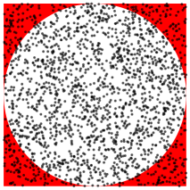
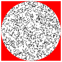
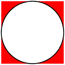
Figure 4.2: Uniform sampling of the circle $\mathbb{S}^{1}$ by rejection sampling. First, the unit square $[-1,1]^{2}$ is uniformly sampled (here, with $2000$ samples). Then all samples $p$ with $\|p\|>1$ in the red domain are rejected. Finally, the remaining samples in the unit disk are normalized, i.e., $p\mapsto\frac{p}{\|p\|}\in\mathbb{S}^{1}$. This yields a uniform distribution on the boundary circle $\mathbb{S}^{1}$. Although this approach can be generalized to higher-dimensional spheres its performance does not scale to high dimensions.

We recall that $\mathbb{S}^{3}$ is a Lie group double cover of $\operatorname{SO}(3)$. A uniform distribution on a compact Lie group is defined in terms of the (normalized) Haar measure of the group, see, e.g., [2, p. 9]. Such a measure is invariant with respect to the left (or right) group multiplication and is unique up to a constant multiple. For an introduction to the Haar measure on Lie groups, see, e.g., [24, p. 179-194]. It is well-known that the Lebesgue measure $\,{\rm dV}_{\mathbb{S}^{3}}$ is a bi-invariant (non-normalized) Haar measure for the Lie group of unit quaternions.

Theorem 4.2 (Uniformly distributed random variables on $\operatorname{SO}(3)$).

Let $X_{\mathbb{S}^{3}}$ be a uniformly distributed random variable on $\mathbb{S}^{3}$ and $\pi:\mathbb{S}^{3}\to\operatorname{SO}(3)$ the covering homorphism defined in (2.10). Then the random variable $X_{\operatorname{SO}(3)}\coloneqq\pi\circ X_{\mathbb{S}^{3}}$ is uniformly distributed with respect to the (normalized) Haar measure on $\operatorname{SO}(3)$.

Proof.

This is well-known, see, e.g., [83]. $\blacksquare$

Essentially, the covering homomorphism $\pi:\mathbb{S}^{3}\to\operatorname{SO}(3)$ induces a bi-invariant Riemannian metric on $\operatorname{SO}(3)$ via the pullback $\big{<}\cdot,\,\cdot\big{>}_{\operatorname{SO}(3)}\coloneqq(\pi^{-1})^{*}\big{<}\cdot,\,\cdot\big{>}_{\mathbb{S}^{3}}$. Note that the bi-invariant metric on $\operatorname{SO}(3)$ is unique up to scalar multiples since the Lie-algebra $\operatorname{\mathfrak{so}}(3)$ is simple. With respect to the pullback metric, $\pi$ is a local isometry. Further, since $\pi$ is a covering map, the pullback of the invariant surface volume measure on $\mathbb{S}^{3}$ given by $(\pi^{-1})^{*}\,{\rm dV}_{\mathbb{S}^{3}}$ induces an invariant measure, i.e., a Haar measure, on $\operatorname{SO}(3)$.

On a sidenote, the use of Riemannian metrics and geodesics on (matrix) Lie groups in applications is currently an active research area, since the computational costs of geometric methods are no longer prohibitive. For some interesting recent applications to strain measures in mechanics, see, e.g., [64]. Another interesting recent usecase for geodesics on the group of unit quaternions is the simulation of eye movements, see [72].

We now briefly describe the sampling strategies for the computational validation.

Remark 4.3 (Sampling the group of rotations $\operatorname{SO}(3)$).

Based on the method described in Theorem 4.2, we have computed a set of samples $\mathcal{Q}\subset\mathbb{S}^{3}$ consisting of $4.629.171$ uniformly distributed unit quaternions.

Remark 4.4 (Sampling strategy for $F\in\operatorname{GL}^{+}(3)$).

We have generated a stream of matrices with uniformly distributed coefficients $F_{ij}\in[-\frac{\operatorname{\rho_{\mu,\,\mu_{c}}}}{2},\frac{\operatorname{\rho_{\mu,\,\mu_{c}}}}{2}]$, $1\leq i,j\leq 3$ and discarded all samples with ${\operatorname{det}[{F}]}<0$. From the remaining samples, we have selected the first $1.000$ samples in $\mathrm{Dom}^{\mathrm{C}}_{\mu,\mu_{c}}$ and $\mathrm{Dom}^{\mathrm{NC}}_{\mu,\mu_{c}}$, respectively, and collected them in two sets $\mathcal{F}^{\mathrm{C}}_{\mu,\mu_{c}}$ and $\mathcal{F}^{\mathrm{NC}}_{\mu,\mu_{c}}$.

Remark 4.5 (Limitations of the sampling strategy for $F\in\operatorname{GL}^{+}(3)$).

For performance reasons our sampling strategy takes our expectations into account right from the onset. This can be seen as a limitation. Further, our validation is inherently limited to compact subsets of $\operatorname{GL}^{+}(3)$. However, this particular strategy, heuristically produces a reasonable resolution for parameters $F\in\operatorname{GL}^{+}(3)$ in the vicinity of the branching condition $\sigma_{1}+\sigma_{2}=\operatorname{\rho_{\mu,\,\mu_{c}}}$ (cf. our Figure 4.4). Based on the predictions of the analysis of our proposed optimal Cosserat rotations presented in Section 3, this is without doubt the most interesting parameter sector.

We are now finally in the position to expose our computational validation strategy for the global optimality of the formula $\operatorname{rpolar}^{\pm}_{\mu,\mu_{c}}(F)$ stated in Corollary 3.6; cf. also Remark 3.4 and Remark 3.5 for a short review of the geometric interpretation of the optimal Cosserat rotations. It is important to note that the presented validation scheme is based on the lift W^♯_μ,μ_c(q ;F) ≔W_μ,μ_c(π(q) ;F) .

This formulation is based on the original Cosserat-shear stretch energy $\operatorname{W_{\mu,\mu_{c}}}(R\,;F)$, precisely as it appears in the statement of Problem 1.1. Clearly, this allows to validate the consistency of the simplifications leading us to Problem 1.5 in Section 1. This approach also implies that the image of the covering homomorphism $\pi:\mathbb{S}^{3}\to\operatorname{SO}(3)$ corresponds to an absolute rotation $\pi(q)=R$.

Let us now present our

Computational Validation 4.6.

Let the sample sets $\mathcal{Q}\subset\mathbb{S}^{3}$ and $\mathcal{F}_{\mu,\mu_{c}}\coloneqq\mathcal{F}_{\mu,\mu_{c}}^{\mathrm{C}}\cup\mathcal{F}_{\mu,\mu_{c}}^{\mathrm{NC}}\subset\operatorname{GL}^{+}(3)$ be as previously defined and set the numerical tolerance $\mathrm{tol}=10^{-4}$. Then for all $\mu>0$ and $\mu_{c}\geq 0$ (which we have tested) the following relation holds:

$$\forall F\in\mathcal{F}_{\mu,\mu_{c}}:\quad\pi\left(\mathchoice{\underset{q\in\mathcal{Q}}{\operatorname{arg\,min}}\,{W^{\sharp}_{\mu,\mu_{c}}(q\,;F)}}{\operatorname{arg\,min}_{q\in\mathcal{Q}}\,{W^{\sharp}_{\mu,\mu_{c}}(q\,;F)}}{}{}\right)\quad=_{\mathrm{tol}}\quad\operatorname{rpolar}^{\pm}_{\mu,\mu_{c}}(F)\;,$$ (4.2)

where $R_{1}=_{\mathrm{tol}}R^{\pm}_{2}\Longleftrightarrow\min_{\pm}\left\lVert R_{1}-R^{\pm}_{2}\right\rVert<\mathrm{tol}$, $R_{1},R^{\pm}_{2}\in\operatorname{SO}(3)$.

The following procedure is equivalent, but more explicit. It also corresponds more closely to our actual implementation:

$$\forall F\in\mathcal{F}_{\mu,\mu_{c}}^{\mathrm{C}}:\quad\operatorname{R_{\rm p}}(F)^{T}\cdot\pi\left(\mathchoice{\underset{q\in\mathcal{Q}}{\operatorname{arg\,min}}\,{W^{\sharp}_{\mu,\mu_{c}}(q\,;F)}}{\operatorname{arg\,min}_{q\in\mathcal{Q}}\,{W^{\sharp}_{\mu,\mu_{c}}(q\,;F)}}{}{}\right) \quad=_{\mathrm{tol}}\quad\{{\boldsymbol{\mathbbm{1}}}\}\;,$$ (4.3)

$$\forall F\in\mathcal{F}_{\mu,\mu_{c}}^{\mathrm{NC}}:\quad\operatorname{R_{\rm p}}(F)^{T}\cdot\pi\left(\mathchoice{\underset{q\in\mathcal{Q}}{\operatorname{arg\,min}}\,{W^{\sharp}_{\mu,\mu_{c}}(q\,;F)}}{\operatorname{arg\,min}_{q\in\mathcal{Q}}\,{W^{\sharp}_{\mu,\mu_{c}}(q\,;F)}}{}{}\right) \quad\equiv_{\mathrm{tol}}\quad[\hat{\beta}^{\pm}_{\mu,\mu_{c}}(F),q_{3}(F)]\;.$$

In order to clarify the meaning of the notation $\equiv_{\mathrm{tol}}$, let $[\hat{\beta}^{\pm}_{\mu,\mu_{c}}(F),q_{3}(F)]\equiv R^{\pm}_{2}\in\operatorname{SO}(3)$, then $R_{1}\equiv_{\mathrm{tol}}[\hat{\beta}^{\pm}_{\mu,\mu_{c}}(F),q_{3}(F)]\Longleftrightarrow R_{1}=_{\mathrm{tol}}R_{2}^{\pm}$; cf. also Remark 3.5.

Remark 4.7 (Additional verification by a Riemannian Newton–scheme (W. Müller)).

For some selected values of $F\in\operatorname{GL}^{+}(3)$, W. Müller (then at Karlsruhe Institute of Technology [55]), has verified that the proposed formula $\operatorname{rpolar}^{\pm}_{\mu,\mu_{c}}(F)$ is a critical point for the Cosserat shear–stretch energy. He successfully approximated our proposed optimal Cosserat rotations up to machine accuracy by using a Riemannian Newton–scheme for the solution of the Euler–Lagrange equations on $\operatorname{SO}(3)$. Perturbations of the starting values of the Newton–iteration did not indicate the existence of alternative solutions realizing lower energy levels.

In Figure 4.4, we present multiple plots of the energy-minimizing relative rotation angles $\hat{\beta}_{\mu,\mu_{c}}$ obtained by stochastic (Monte Carlo) minimization. We show plots for different values of ${\mu,\mu_{c}}$. A corresponding, in itself rather uninteresting, plot for the classical limit case $(\mu,\mu_{c})=(1,0)$ is depicted in Figure 4.3 for direct comparison. Both figures match our expectations raised by Figure 3.2 very well and the resolution does improve with higher sample counts. It is instructive to compare these figures with the optimal relative rotation angles for optimal planar Cosserat rotations presented in Part I of the present contribution, see [29].

Parameters: $(\mu,\mu_{c})=(1,1)$

$\rho_{1,1}=\infty$

Figure 4.3: Optimal relative rotation angle $\hat{\beta}_{1,1}^{\rm MC}$ obtained from stochastic (Monte Carlo) minimization for the classical limit case $\mu=\mu_{c}=1$. We observe that the relative rotation angle vanishes up to numerical accuracy, since the polar factor $\operatorname{R_{\rm p}}(F)$ is always optimal in perfect accordance with Grioli’s theorem, see [69] and [29, Cor. 2.4, p. 5]. More precisely, this corresponds to the prediction $\hat{\beta}^{\pm}_{1,1}(\sigma_{1}+\sigma_{2})=0$. For multiple examples from the non-classical parameter range $\mu>\mu_{c}\geq 0$, see Figure 4.4 on page 4.4.

Parameters: $(\mu,\mu_{c})=(1,0)$

$\rho_{1,0}=2$

Parameters: $(\mu,\mu_{c})=(1,\frac{1}{4})$

$\rho_{1,\frac{1}{4}}=\frac{8}{3}$

Parameters: $(\mu,\mu_{c})=(1,\frac{1}{2})$

$\rho_{1,\frac{1}{2}}=4$

Figure 4.4: Optimal relative rotation angles $\hat{\beta}^{\rm MC}_{\mu,\mu_{c}}$ for multiple non-classical values $\mu>\mu_{c}\geq 0$. The angles are obtained by stochastic (Monte Carlo) minimization of $W_{\mu,\mu_{c}}(R\,;F)$. The dashed blue curve shows the predicted value for $\hat{\beta}_{1,0}^{\pm}(\sigma_{1}+\sigma_{2})$ and the dashed red line marks the expected bifurcation point at $\rho_{\mu,\mu_{c}}$. For a direct comparison, we provide Figure 4.3 on page 4.3 which shows the classical limit case $(\mu,\mu_{c})=(1,1)$; see also Figure 3.2 on page 3.2 for an illustration and a more precise description of the bifurcation behavior predicted by our proposed formula $\operatorname{rpolar}^{\pm}_{\mu,\mu_{c}}(F)$.

5 Conclusion

The reduced Cosserat shear–stretch energy $\operatorname{W^{\rm red}_{\mu,\mu_{c}}}$ for which we have finally obtained an explicit form in Theorem 3.11 admits an interesting abstract interpretation in mechanics. In order to reveal this, let us first assume that the microrotations $R$ are spatially decoupled. This is the case when the length scale parameter $L_{\rm c}$ in the full Cosserat model, i.e., including a curvature energy contribution, is extremely small or zero. Let us furthermore assume that ${\operatorname{det}[{F}]}=1$, i.e., that the amount of volume distortion is negligible and that a specimen $\Omega$ of this material is subjected to a given deformation $\varphi:\Omega\to\varphi(\Omega)$ with deformation gradient $F\coloneqq\nabla\!\mathbf{\varphi}\in\operatorname{GL}^{+}(3)$. Then the total reduced Cosserat shear–stretch energy obtained by integration of the local density given by

$$\int\nolimits_{\Omega}\operatorname{W^{\rm red}_{\mu,\mu_{c}}}(F)\,{\rm dV}\;\coloneqq\;\int\nolimits_{\Omega}\min_{R\,\in\,\operatorname{SO}(3)}\operatorname{W_{\mu,\mu_{c}}}(R\,;F)\,{\rm dV}$$ (5.1)

corresponds precisely to the total energetic response which is generated if the field of microrotations $R$ in the specimen instantaneously aligns itself with the field of locally optimal Cosserat rotations $\operatorname{rpolar}^{\pm}_{\mu,\mu_{c}}(\nabla\!\mathbf{\varphi})$. It is important to observe that the the field of optimal Cosserat rotations is purely induced by the deformation mapping $\varphi$ on which it depends by local energy minimization and does not otherwise depend on boundary conditions, exterior forces, etc.

A Cosserat material which conforms to the previous description can be nicely embedded into a classical framework due to G. Capriz, the description of which is one of many shimmering pearls to be found in the impressive body of his work on micropolar materials, see, e.g., [15, 13], and it is with delight that we summarize it in a brief

Remark 5.1 (Continua with latent microstructure in the sense of Capriz).

In his paper [12, p.49], G. Capriz introduces the notion of a continuum with latent microstructure as follows:

“I say that the microstructure is latent when, though its effects are felt in the balance equations, all relevant quantities can be expressed in terms of geometric and kinematic quantities pertaining to apparent placements.”

Capriz then gives a more precise definition of the properties a latent microstructure needs to satisfy. We shall only repeat the first two: “There is no inertia connected with the microstructure.”, and, “There are no exterior body actions on the microstructure.” In other words, a latent microstructure is coupled with a deformation $\varphi$ in an instantaneous way.

The reduced Cosserat shear-stretch energy $\operatorname{W^{\rm red}_{\mu,\mu_{c}}}(F)$ can be considered as the energetic answer of a medium with a rotational microstructure that instantaneously reorganizes its field of microrotations $R:\Omega\to\operatorname{SO}(3)$ as an energy-minimizing $\operatorname{rpolar}^{\pm}_{\mu,\mu_{c}}(F)$-field. This is an example for a latent microstructure in the sense of Capriz.

From a more general perspective, a Cosserat continuum can also be considered as a special case of a so-called micromorphic model, see, e.g., [66, 61] and [51]. Let us, as before, set the length scale parameter $L_{\rm c}$ governing the curvature contribution to zero. We then observe that such an approach always leads to an algebraic side condition, in our case it is given by the equation (2.17), which replaces the partial differential equation for the micro-distortion field. This is another, more general, example of a continuum with latent microstructure in the sense of Capriz, compare, e.g., [14], due to G. Capriz himself and also [51].

Note that in [22] and [21], the authors – who are apparently unaware of this established and relatively straightforward interpretation – have, in our opinion, recently reintroduced the framework of materials with latent microstructure due to G. Capriz for such micromorphic continuum models under the new name of a hyperelastic material with “internal balance” and an “internally balanced solid”, respectively.

We now continue our conclusion with some thoughts on possible generalizations of our present results.

Remark 5.2 (On generalizations to higher dimensions $n\geq 4$).

Our solution approach is quite specifically tailored to dimension $n=3$ since it relies on the covering of $\operatorname{SO}(3)$ by the unit quaternions $\mathbb{S}^{3}\subset\operatorname{\mathbb{H}}$. It seems reasonable to assume that the particularly simple geometry of $\mathbb{S}^{3}$ lies at the root of the explicit solvability of the Euler–Lagrange equations. The so-called Sphere Theorem states that the only spheres that admit a connected compact Lie group structure are $\mathbb{S}^{1}$ and $\mathbb{S}^{3}$, see, e.g., [42, p.289]. Thus, for $n>3$, there is no hope at all to recover the particularly simple constellation we have quite successfully exploited here. Still, there is a generalization of the unit quaternions, namely the so-called spin groups $\mathrm{Spin}(n)$. These groups are two-fold covers of $\operatorname{SO}(n)$ and closely related to Clifford algebras, see, e.g., [46] and [23]. In principle, such techniques might be appropriate for a generalization of our present results to higher dimensions, but they are out of reach for us.

Although our exact solution approach does not generalize to higher dimensions, it seems obvious that the reduced Problem 1.5 is a very good starting point for the solution of Problem 1.1 in dimensions $n\geq 4$. Given this particular form, it seems very likely that the minimizers in higher dimensions can also be characterized in terms of the eigenvectors of $U=QDQ^{T}$ and the singular values $\sigma_{i}$, $1\leq i\leq n$, of $F\in\operatorname{GL}^{+}(n)$. Similar to the rather simplistic random sampling strategy we have employed here, it might certainly be worthwhile to carry out an initial investigation based on a suitable Monte Carlo random sampling approach which is suitable for higher dimensions, see, e.g., [16]. On a related note, we have to dampen expectations regarding extensions to anisotropic formulations. These seem to be completely out of reach, since a reduction to a formulation in singular values is then impossible, see [58] and [73].

Another interesting question which is raised by our findings is whether the maximal mean planar stretch and strain “measures”, i.e., $u^{\rm mmp}(F)$ and $s^{\rm mmp}(F)$, as defined in Definition 3.1 – which appear to be such natural concepts in our particular context – are just artifacts of our derivation. The same holds for the plane of maximal strain $\mathrm{P}^{\rm mp}(F)$ introduced in Definition 3.3. Are there real-world materials or material models which can be precisely or at least approximately characterized by, e.g., slip in the plane of maximal strain $\mathrm{P}^{\rm mp}(F)$? Currently, we are not aware of any such materials or models.

In good hope that the presented mechanisms and computational strategies will be at least helpful for the derivation of closed-form solutions for Problem 1.1 in dimensions $n\geq 3$ and that these will match our proposed formula $\operatorname{rpolar}^{\pm}_{\mu,\mu_{c}}(F)$ presented in Corollary 3.6 for $n=3$, we conclude our present contribution with a last

Remark 5.3 (Final remark).

As regards suitable values of the Cosserat couple modulus $\mu_{c}\geq 0$, our development shows clearly that there are ultimately only 3 values of particular interest, namely

$$\mu_{c}\;=\;0\;,\quad\quad\mu_{c}\;=\;\mu\;,\quad\quad\text{and}\quad\quad\mu_{c}\;=\;+\infty\;. \blacksquare$$

Appendix A Appendix (list of critical points)

We now detail our computer assisted strategy for the computation of the critical points for the Lagrange function $\widehat{L}_{1,0}$. We recall that the Euler–Lagrange equations simplify considerably if one (or more) of the quaternion coefficients $w,x,y$ or $z$ vanishes. This is reflected in the solution set computed by Mathematica.

We recall our shorthand notation for sums and differences of singular values for parameters $F\in\operatorname{GL}^{+}(n)$ introduced in Section 2:

$$s_{ij}\coloneqq\sigma_{i}+\sigma_{j}\quad\text{and}\quad d_{ij}\coloneqq\sigma_{i}-\sigma_{j}\;,\quad i,j=1,2,3\;.$$

A.1 Computation of critical points of the Lagrange function $\widehat{L}_{1,0}$

In order to solve the Euler–Lagrange equations in quaternion representation (2.16), we have used the Reduce command in Mathematica. This command returns 130 critical points for the Lagrange function $\widehat{L}_{1,0}$. The solution set is enlarged by particular solutions satisfying certain algebraic relations among the parameters $\sigma_{i}$, $i=1,\ldots,3$. In order to exclude these cases, we have made the following assumptions

$$\sigma_{i}\neq 0\;,\quad s_{ij}\coloneqq\sigma_{i}+\sigma_{j}\neq 0\;,\quad\text{and}\quad d_{ij}\coloneqq\sigma_{i}-\sigma_{j}\neq 0\;,\quad i,j=1,2,3,\;i\neq j\;.$$ (1.1)

These assumptions can be passed to the Reduce command in the form of a so-called AssumptionList. This is a standard procedure. With these assumptions Mathematica successfully symbolically reduces the full solution set comprised of 130 critical points to 32 critical points. Note that a strict ordering of the parameters $\sigma_{1}>\sigma_{2}>\sigma_{3}>0$ implies that all of these assumptions in (1.1) are satisfied. We shall refer to the 32 branches so obtained as the set of generic solutions, since they coincide with the output of the Solve command. Due to this procedure, the possibility of multiple singular values of $F$ and the degeneracy of ${\operatorname{det}[{F}]}=0$ are explicitly excluded.

Remark A.1 (Completeness of the solution set).

We want to stress that we present manually refined results obtained via the computational algebra system (CAS) Mathematica. Currently, we cannot prove that our solution set is complete, but this is quite probably the case as our extensive validation shows.

It might be an interesting challenge for an expert in (computational) algebraic geometry to prove that the presented list of generic solutions to the polynomial system (2.16) is in fact complete.

Note that the computations can also be based on the alternative continuation $\pi^{\prime}:\operatorname{\mathbb{H}}\to\operatorname{SO}(3)$ which produces slightly different Euler–Lagrange equations but yields the same full and generic solution sets.

In order to describe the set of generic solutions, we introduce two auxiliary coefficient functions

$$c_{A}(t)\coloneqq\sqrt{\frac{1}{2}+\frac{1}{t}}\;,\quad\text{and}\quad c_{B}(t)\coloneqq\sqrt{\frac{1}{2}-\frac{1}{t}}\;.$$ (1.2)

It is important to note that the function $c_{B}(t)$ is only real-valued for $t\in[2,\infty)$. The generic solutions are critical tuples of complex variables $(w,x,y,z,\lambda)\in\mathbb{C}^{5}$, i.e., the solutions obtained by Mathematica are complex-valued. It turns out that the critical tuples are real-valued if and only if the radicands in (1.2) are non-negative which allows to deduce corresponding domains of definition for the critical branches.

Remark A.2 (Covering symmetry).

For any critical pair $(\hat{q},\lambda)$, the pair $(-\hat{q},\lambda)$ is also a critical point for the Lagrange function $\widehat{L}_{1,0}$. The associated reduced energy levels are identical.

Due to this antipodal symmetry, it suffices to restrict the following presentation to $16$ solutions. For their exposition, we have decided to introduce three categories.

A.1.1 Type I (of critical points)

Characterization: Precisely one of the coefficients $w,x,y$ and $z$ of $\hat{q}(w,x,y,z)$ is non-zero. The solutions are independent of the parameters $\sigma_{i}$, $i=1,2,3$.

These correspond to the following energy-minmizing relative rotations:

$$\begin{matrix}[l]\hat{q}_{{\mathrm{I}},1}&\coloneqq&(1,\,0,\,0,\,0)&\equiv&\left[0,\,\quad\text{any}\quad\right]&\equiv&{\boldsymbol{\mathbbm{1}}}_{3}&=&Q_{1}\;,\\ \hat{q}_{{\mathrm{I}},2}&\coloneqq&(0,\,1,\,0,\,0)&\equiv&\left[\pi,(1,\,0,\,0)\right]&\equiv&\operatorname{diag}(\phantom{-}1,\,-1,\,-1)&=&Q_{2}\;,\\ \hat{q}_{{\mathrm{I}},3}&\coloneqq&(0,\,0,\,1,\,0)&\equiv&\left[\pi,(0,\,1,\,0)\right]&\equiv&\operatorname{diag}(-1,\,\phantom{-}1,\,-1)&=&Q_{3}\;,\\ \hat{q}_{{\mathrm{I}},4}&\coloneqq&(0,\,0,\,0,\,1)&\equiv&\left[\pi,(0,\,0,\,1)\right]&\equiv&\operatorname{diag}(-1,\,-1,\,\phantom{-}1)&=&Q_{4}\;.\end{matrix}$$ (1.3)

Note that the relative rotation represented by $\hat{q}_{{\mathrm{I}},1}\equiv{\boldsymbol{\mathbbm{1}}}_{3}$ corresponds to the polar factor $\operatorname{R_{\rm p}}(F)$.

For the Lagrange multiplier $\lambda$, we obtain the associated critical values

$$\lambda_{\mathrm{I},1}\coloneqq 0\;,\quad\lambda_{\mathrm{I},2}\coloneqq\sigma_{2}^{2}+\sigma_{3}^{2}+4\,s_{23}\;,\quad\lambda_{\mathrm{I},3}\coloneqq\sigma_{3}^{2}+\sigma_{1}^{2}+4\,s_{31}\;,\quad\text{and}\quad\lambda_{\mathrm{I},4}\coloneqq\sigma_{1}^{2}+\sigma_{2}^{2}+4\,s_{12}\;.$$ (1.4)

The realized energy levels of the lifted energy are given by:

$$\widehat{W}_{1,0}^{\sharp}(\hat{q}_{{\mathrm{I}},1}\,;D) =(\sigma_{1}-1)^{2}+(\sigma_{2}-1)^{2}+(\sigma_{3}-1)^{2}\;,$$ (1.5)

$$\widehat{W}_{1,0}^{\sharp}(\hat{q}_{{\mathrm{I}},2}\,;D) =(\sigma_{1}+1)^{2}+(\sigma_{2}+1)^{2}+(\sigma_{3}-1)^{2}\;,$$

$$\widehat{W}_{1,0}^{\sharp}(\hat{q}_{{\mathrm{I}},3}\,;D) =(\sigma_{1}-1)^{2}+(\sigma_{2}+1)^{2}+(\sigma_{3}+1)^{2}\;,$$

$$\widehat{W}_{1,0}^{\sharp}(\hat{q}_{{\mathrm{I}},4}\,;D) =(\sigma_{1}+1)^{2}+(\sigma_{2}-1)^{2}+(\sigma_{3}+1)^{2}\;.$$

The solutions of the first type are globally defined.

A.1.2 Type II (of critical points)

Characterization: Precisely two of the coefficients $x,y,z$ of $\hat{q}(w,x,y,z)$ vanish. Further, the solution only depends on pairwise sums of the singular values $\sigma_{i}$, $i=1,2,3$.

These correspond to the following energy-minmizing relative rotations:

$$\begin{matrix}[l]\hat{q}^{\pm}_{{\mathrm{II}},1}\coloneqq\left(c_{A}(s_{12}),\,0,\,0,\pm c_{B}(s_{12})\right)&\equiv&\left[\pm\arccos(2/s_{12}),(0,\,0,\,1)\right]\;,\\[4.0pt] \hat{q}^{\pm}_{{\mathrm{II}},2}\coloneqq\left(c_{A}(s_{23}),\,\pm c_{B}(s_{23}),\,0,\,0\right)&\equiv&\left[\pm\arccos(2/s_{23}),(1,\,0,\,0)\right]\;,\\[4.0pt] \hat{q}^{\pm}_{{\mathrm{II}},3}\coloneqq\left(c_{A}(s_{31}),\,0,\,\pm c_{B}(s_{31}),\,0\right)&\equiv&\left[\pm\arccos(2/s_{31}),(0,\,1,\,0)\right]\;.\end{matrix}$$ (1.6)

For the Lagrange multiplier $\lambda$, we obtain the associated critical values

$$\lambda^{\pm}_{\mathrm{II},1}\coloneqq d_{12}^{2}\left(\frac{s_{12}-2}{s_{12}}\right)\;,\quad\lambda^{\pm}_{\mathrm{II},2}\coloneqq d_{23}^{2}\left(\frac{s_{23}-2}{s_{23}}\right)\;,\quad\text{and}\quad\lambda^{\pm}_{\mathrm{II},3}\coloneqq d_{31}^{2}\left(\frac{s_{31}-2}{s_{31}}\right)\;.$$ (1.7)

The realized energy levels of the lifted energy are given by:

$$\widehat{W}_{1,0}^{\sharp}(\hat{q}^{\pm}_{{\mathrm{II}},1}\,;D)=\frac{1}{2}(\sigma_{1}-\sigma_{2})^{2}+(\sigma_{3}-1)^{2}\;,$$ (1.8)

$$\widehat{W}_{1,0}^{\sharp}(\hat{q}^{\pm}_{{\mathrm{II}},2}\,;D)=\frac{1}{2}(\sigma_{2}-\sigma_{3})^{2}+(\sigma_{1}-1)^{2}\;,$$

$$\widehat{W}_{1,0}^{\sharp}(\hat{q}^{\pm}_{{\mathrm{II}},3}\,;D)=\frac{1}{2}(\sigma_{3}-\sigma_{1})^{2}+(\sigma_{2}-1)^{2}\;.$$

The solutions of the second type are defined for $s_{ij}\in[2,\infty)$, $i,j=1,2,3$.

A.1.3 Type III (of critical points)

Characterization: The coefficient $w$ vanishes together with exactly one of the remaining coefficients $x,y,z$ of $\hat{q}(w,x,y,z)$. Further, the solution only depends on pairwise differences of the singular values $\sigma_{i}$, $i=1,2,3$.

These correspond to the following energy-minmizing relative rotations:

$$\begin{matrix}[l]\hat{q}^{\pm}_{{\mathrm{III}},1}\coloneqq\left(0,\,c_{A}(d_{12}),\,\pm c_{B}(d_{12}),\,0\right)&\equiv&\left[\pi,\left(c_{A}(d_{12})^{-\frac{1}{2}},\,\pm c_{B}(d_{12})^{\frac{1}{2}},\,0\right)\right]\;,\\[6.0pt] \hat{q}^{\pm}_{{\mathrm{III}},2}\coloneqq\left(0,\,0,\,c_{A}(d_{23}),\,\pm c_{B}(d_{23})\right)&\equiv&\left[\pi,\left(0,\,c_{A}(d_{23})^{-\frac{1}{2}},\,\pm c_{B}(d_{23})^{\frac{1}{2}}\right)\right]\;,\\[6.0pt] \hat{q}^{\pm}_{{\mathrm{III}},3}\coloneqq\left(0,\,c_{A}(-d_{31}),\,0,\,\pm c_{B}(-d_{31})\right)&\equiv&\left[\pi,\left(c_{A}(-d_{31})^{-\frac{1}{2}},\,0,\,\pm c_{B}(-d_{31})^{\frac{1}{2}}\right)\right]\;.\end{matrix}$$ (1.9)

For the Lagrange multiplier $\lambda$, we obtain the associated critical values

$$\lambda^{\pm}_{\mathrm{III},1} \coloneqq\quad 4\,\sigma_{3}(1+\sigma_{3})+(s_{23}-2)s_{23}\;,$$ (1.10)

$$\lambda^{\pm}_{\mathrm{III},2} \coloneqq\quad 4\,\sigma_{1}(1+\sigma_{1})+(s_{12}-2)s_{12}\;,$$

$$\lambda^{\pm}_{\mathrm{III},3} \coloneqq\quad 4\,\sigma_{2}(1+\sigma_{2})+(s_{31}-2)s_{31}\;.$$

The realized energy levels of the lifted energy are given by

$$\widehat{W}_{1,0}^{\sharp}(\hat{q}^{\pm}_{{\mathrm{III}},1}\,;D) =\quad\frac{1}{2}(\sigma_{1}+\sigma_{2})^{2}+(\sigma_{3}+1)^{2}\;,$$ (1.11)

$$\widehat{W}_{1,0}^{\sharp}(\hat{q}^{\pm}_{{\mathrm{III}},2}\,;D) =\quad\frac{1}{2}(\sigma_{2}+\sigma_{3})^{2}+(\sigma_{1}+1)^{2}\;,$$

$$\widehat{W}_{1,0}^{\sharp}(\hat{q}^{\pm}_{{\mathrm{III}},3}\,;D) =\quad\frac{1}{2}(\sigma_{3}+\sigma_{1})^{2}+(\sigma_{2}+1)^{2}\;.$$

The solutions of the third type are defined for $d_{ij}\in[2,\infty)$, $i<j$, $i,j=1,2,3$.

Remark A.3 (On second order conditions).

We have succeeded to compute the signs of the principal minors of the so-called bordered Hessian $\mathrm{H}_{(\hat{q},\lambda)}\widehat{L}_{1,0}(\hat{q},\lambda\,;D)$ evaluated at the previously presented $32$ critical points. This allows to carry out an analysis of the second order conditions for local constrained extrema based on an analysis of the sign changes of the principal minors of the bordered Hessian. The procedure in the constrained case is different but similar to the well-known procedure in the unconstrained case [19, 39].

References

- [1] P.-A. Absil, R. Mahony, and R. Sepulchre. Optimization Algorithms on Matrix Manifolds. Princeton University Press, 2009.
- [2] D. Applebaum. Probability on Compact Lie Groups. Probability Theory and Stochastic Modelling. Springer, 2014.
- [3] A. Baker. Matrix Groups: An Introduction to Lie Group Theory. Undergraduate Mathematics. Springer, 2012.
- [4] M. Bîrsan and P. Neff. Existence of minimizers in the geometrically non-linear 6-parameter resultant shell theory with drilling rotations. Math. Mech. Solids, DOI: 10.1177/1081286512466659, 2013.
- [5] M. Bîrsan and P. Neff. Existence theorems in the geometrically non-linear 6-parameter theory of elastic plates. J. Elasticity, DOI 10.1007/s10659-012-9405-2, 2013.
- [6] T. Blesgen. Deformation patterning in the framework of large-strain Cosserat plasticity. Model. Simul. Mater. Sc., 21(3):035001, 2013.
- [7] T. Blesgen. Deformation patterning in three-dimensional large-strain Cosserat plasticity. Mech. Res. Comm., 62:37 – 43, 2014.
- [8] J. Bochnak, M. Coste, and M.-F. Roy. Real Algebraic Geometry, volume 36 of Ergebnisse der Mathematik und ihrer Grenzgebiete. 3. Folge / A Series of Modern Surveys in Mathematics. Springer, 2013.
- [9] C. G. Boehmer, P. Neff, and B. Seymenoglu. Soliton-like solutions based on geometrically nonlinear Cosserat micropolar elasticity. arXiv preprint arXiv:1503.08860, 2015. http://arxiv.org/pdf/1503.08860v1, to appear in Wave Motion.
- [10] T. Bröcker and T. tom Dieck. Representations of Compact Lie Groups. Graduate Texts in Mathematics. Springer, 2003.
- [11] H. Bufler. The Biot stresses in nonlinear elasticity and the associated generalized variational principles. Ing. Arch., 55(6):450–462, 1985.
- [12] G. Capriz. Continua with latent microstructure. Arch. Ration. Mech. Anal., 90:43–56, 1985.
- [13] G. Capriz. Continua with Microstructure, volume 35 of Springer Tracts in Natural Philosophy. Springer-Verlag, New York, 1989.
- [14] G. Capriz and M. Brocato. Polycrystalline microstructure. Rend. Sem. Mat. Univ. Politec. Torino, 58(1):49–56, 2000.
- [15] G. Capriz and P. Podio Guidugli. Formal structure and classification of theories of oriented materials. Ann. Mat. Pura Appl. (4), 115(1):17–39, 1977.
- [16] A. L. Carlos, J.-C. Massé, and L. P. Rivest. A statistical model for random rotations. J. Multivariate Anal., 97(2):412 – 430, 2006.
- [17] E. Cosserat and F. Cosserat. Théorie des Corps Déformables. Librairie Scientifique A. Hermann et Fils (engl. translation by D. Delphenich 2007, available online at https://www.uni-due.de/~hm0014/Cosserat_files/Cosserat09_eng.pdf), reprint 2009 by Hermann Librairie Scientifique, ISBN 978 27056 6920 1, Paris, 1909.
- [18] D. A. Cox, J. Little, and D. O’Shea. Using Algebraic Geometry, volume 185 of Graduate Texts in Mathematics. Springer, 2006.
- [19] G. Debreu. Definite and semidefinite quadratic forms. Econometrica, pages 295–300, 1952.
- [20] W. Decker, G.-M. Greuel, G. Pfister, and H. Schönemann. Singular 4.0.2 — A computer algebra system for polynomial computations. http://www.singular.uni-kl.de, 2015.
- [21] H. Demirkoparan and T. J. Pence. Finite stretching and shearing of an internally balanced elastic solid. J. Elasticity, 121(1):1–23, 2015.
- [22] H. Demirkoparan, T. J. Pence, and H. Tsai. Hyperelastic internal balance by multiplicative decomposition of the deformation gradient. Arch. Ration. Mech. Anal., 214(3):923–970, 2014.
- [23] C. Doran and A. N. Lasenby. Geometric Algebra for Physicists. Cambridge University Press, 2003.
- [24] J. J. Duistermaat and J. A. C. Kolk. Lie Groups. Universitext. Springer, 2012.
- [25] H. Ebbinghaus, H. Hermes, and F. Hirzebruch. Numbers. Graduate Texts in Mathematics. Springer, 1990.
- [26] V. A. Eremeyev, L. P. Lebedev, and H. Altenbach. Foundations of Micropolar Mechanics. Springer, 2012.
- [27] V. A. Eremeyev and W. Pietraszkiewicz. The nonlinear theory of elastic shells with phase transitions. J. Elasticity, 74:67–86, 2004.
- [28] A. C. Eringen. Microcontinuum Field Theories. Vol. I: Foundations and Solids. Springer, 1999.
- [29] A. Fischle and P. Neff. The geometrically nonlinear Cosserat micropolar shear-stretch energy. Part I: A general parameter reduction formula and energy-minimizing microrotations in 2D. arXiv preprint arXiv:1507.05480, 2015. http://arxiv.org/abs/1507.05480, submitted to Z. angew. Math. Mechanik.
- [30] A. Fischle, P. Neff, and I. Münch. Symmetric Cauchy stresses do not imply symmetric Biot strains in weak formulations of isotropic hyperelasticity with rotational degrees of freedom. Proc. Appl. Math. Mech., 8:10419–10420, 2008.
- [31] S. Forest, G. Cailletaud, and R. Sievert. A Cosserat theory for elastoviscoplastic single crystals at finite deformation. Arch. Mech., 49(4):705–736, 1997.
- [32] K. Gall and H. Sehitoglu. The role of texture in tension–compression asymmetry in polycrystalline NiTi. Int. J. Plast., 15(1):69–92, 1999.
- [33] K. Gall, H. Sehitoglu, Y. I. Chumlyakov, and I. V. Kireeva. Tension–compression asymmetry of the stress–strain response in aged single crystal and polycrystalline NiTi. Acta Mater., 47(4):1203–1217, 1999.
- [34] J. Gallier. Notes on Differential Geometry and Lie Groups. (book in progress), 2015. http://www.cis.upenn.edu/~jean/gbooks/manif.html.
- [35] G. Grioli. Una proprieta di minimo nella cinematica delle deformazioni finite. Boll. Un. Math. Ital., 2:252–255, 1940.
- [36] P. Grohs, H. Hardering, and O. Sander. Optimal a priori discretization error bounds for geodesic finite elements. Found. Comput. Math., pages 1–55, 2013.
- [37] Sir W. R. Hamilton. On a new species of imaginary quantities connected with a theory of Quaternions. In Proceedings of the Royal Irish Academy, volume 2, pages 424–434, 1843. available online at http://www.emis.de/classics/Hamilton/Quatern1.pdf.
- [38] Sir W. R. Hamilton. Elements of Quaternions. Longmans, Green, & Company, 1866. available online at https://archive.org/details/117770258_002.
- [39] M. R. Hestenes. Optimization Theory: The Finite Dimensional Case. Pure and Applied Mathematics. John Wiley & Sons, 1975.
- [40] J. S. Hicks and R. F. Wheeling. An efficient method for generating uniformly distributed points on the surface of an n-dimensional sphere. Commun. ACM, 2(4):17–19, April 1959.
- [41] J. Hilgert and K.-H. Neeb. Lie-Gruppen und Lie-Algebren. Vieweg Verlagsgesellschaft, 1991.
- [42] K. H. Hofmann and S. A. Morris. The Structure of Compact Groups: A Primer for Students-A Handbook for the Expert, volume 25. Walter de Gruyter, 2006.
- [43] J. Jeong, H. Ramézani, I. Münch, and P. Neff. A numerical study for linear isotropic Cosserat elasticity with conformally invariant curvature. Z. Angew. Math. Mech., 89(7):552–569, 2009.
- [44] J. Lankeit, P. Neff, and Y. Nakatsukasa. The minimization of matrix logarithms: On a fundamental property of the unitary polar factor. Lin. Alg. Appl., 449:28–42, 2014.
- [45] J. Lankeit, P. Neff, and F. Osterbrink. Integrability conditions between the first and second Cosserat deformation tensor in geometrically nonlinear micropolar models and existence of minimizers. arXiv preprint arXiv:1504.08003, 2015. http://arxiv.org/pdf/1504.08003v1.
- [46] H. B. Lawson Jr. and M.-L. Michelsohn. Spin Geometry. Oxford University Press, 1989.
- [47] J. M. Lee. Introduction to Smooth Manifolds. Graduate Texts in Mathematics. Springer, 2002.
- [48] G. Marsaglia. Choosing a point from the surface of a sphere. Ann. Math. Statist., 43(2):645–646, 04 1972.
- [49] J. E. Marsden and T. Ratiu. Introduction to Mechanics and Symmetry: A Basic Exposition of Classical Mechanical Systems, volume 17. Springer, 2013.
- [50] L.C. Martins and P. Podio-Guidugli. An elementary proof of the polar decomposition theorem. Amer. Math. Month., 87:288–290, 1980.
- [51] F. Matteo, M. P. Mariano, and E. Spadaro. Multi-value microstructural descriptors for complex materials: analysis of ground states. Arch. Ration. Mech. Anal., 217(3):899–933, 2015.
- [52] G. A. Maugin. On the structure of the theory of polar elasticity. R. Soc. Lond. Philos. Trans. Ser. A Math. Phys. Eng. Sci., 356(1741):1367–1395, 1998.
- [53] A. Montes and M. Wibmer. Gröbner bases for polynomial systems with parameters. J. Symb. Comp., 45(12):1391–1425, 2010.
- [54] M. E. Muller. A note on a method for generating points uniformly on n-dimensional spheres. Commun. ACM, 2(4):19–20, April 1959.
- [55] W. Müller. Numerische Analyse und parallele Simulation von nichtlinearen Cosserat-Modellen. Dissertation in der Fakultät für Mathematik, Karlsruhe, 2009. http://digbib.ubka.uni-karlsruhe.de/volltexte/1000014838.
- [56] I. Münch. Ein geometrisch und materiell nichtlineares Cosserat-Modell - Theorie, Numerik und Anwendungmöglichkeiten. Dissertation in der Fakultät für Bauingenieur-, Geo- und Umweltwissenschaften, Karlsruhe, 2007. http://digbib.ubka.uni-karlsruhe.de/volltexte/1000007371.
- [57] I. Münch, W. Wagner, and P. Neff. Theory and FE-analysis for structures with large deformation under magnetic loading. Comp. Mech., 44(1):93–102, 2009.
- [58] I. Münch, W. Wagner, and P. Neff. Transversely isotropic material: nonlinear Cosserat versus classical approach. Cont. Mech. Thermod., 23(1):27–34, 2011.
- [59] P. Neff. A geometrically exact Cosserat-shell model including size effects, avoiding degeneracy in the thin shell limit. Part I: Formal dimensional reduction for elastic plates and existence of minimizers for positive Cosserat couple modulus. Cont. Mech. Thermod., 16(6):577–628, 2004.
- [60] P. Neff. The Cosserat couple modulus for continuous solids is zero viz the linearized Cauchy-stress tensor is symmetric. Z. Angew. Math. Mech., 86:892–912, 2006.
- [61] P. Neff. Existence of minimizers for a finite-strain micromorphic elastic solid. Proc. Roy. Soc. Edinb. A, 136:997–1012, 2006.
- [62] P. Neff. A finite-strain elastic-plastic Cosserat theory for polycrystals with grain rotations. Int. J. Engng. Sci., 44:574–594, 2006.
- [63] P. Neff, M. Bîrsan, and F. Osterbrink. Existence theorem for geometrically nonlinear Cosserat micropolar model under uniform convexity requirements. J. Elasticity, 121, Issue 1:1–23, 2015.
- [64] P. Neff, B. Eidel, and R. J. Martin. Geometry of logarithmic strain measures in solid mechanics. arXiv preprint arXiv:1505.02203, 2015. http://arxiv.org/pdf/1505.02203v1.
- [65] P. Neff, A. Fischle, and I. Münch. Symmetric Cauchy-stresses do not imply symmetric Biot-strains in weak formulations of isotropic hyperelasticity with rotational degrees of freedom. Acta Mech., 197:19–30, 2008.
- [66] P. Neff and S. Forest. A geometrically exact micromorphic model for elastic metallic foams accounting for affine microstructure. Modelling, existence of minimizers, identification of moduli and computational results. J. Elasticity, 87:239–276, 2007.
- [67] P. Neff and J. Jeong. A new paradigm: the linear isotropic Cosserat model with conformally invariant curvature energy. Z. Angew. Math. Mech., 89(2):107–122, 2009.
- [68] P. Neff, J. Jeong, and A. Fischle. Stable identification of linear isotropic Cosserat parameters: bounded stiffness in bending and torsion implies conformal invariance of curvature. Acta Mech., 211(3-4):237–249, 2010.
- [69] P. Neff, J. Lankeit, and A. Madeo. On Grioli’s minimum property and its relation to Cauchy’s polar decomposition. Int. J. Engng. Sci., 80:209–217, 2014.
- [70] P. Neff and I. Münch. Simple shear in nonlinear Cosserat elasticity: bifurcation and induced microstructure. Cont. Mech. Thermod., 21(3):195–221, 2009.
- [71] P. Neff, Y. Nakatsukasa, and A. Fischle. A logarithmic minimization property of the unitary polar factor in the spectral and Frobenius norms. SIAM J. Matrix Anal. Appl., 35(3):1132–1154, 2014.
- [72] A. Novelia and O. M. O’Reilly. On geodesics of the rotation group . (pending), 2015. electronic preprint available at http://dynamics.berkeley.edu/assets/Geodesics-SO3.pdf.
- [73] A. Pau and P. Trovalusci. Block masonry as equivalent micropolar continua: the role of relative rotations. Acta Mech., 223(7):1455–1471, 2012.
- [74] W. Pietraszkiewicz and V. A. Eremeyev. On vectorially parameterized natural strain measures of the non-linear Cosserat continuum. Int. J. Solids Struct., 46(11):2477–2480, 2009.
- [75] W. Pietraszkiewicz and V.A. Eremeyev. On natural strain measures of the non-linear micropolar continuum. Int. J. Solids Struct., 46:774–787, 2008.
- [76] O. Sander. Geodesic finite elements on simplicial grids. Int. J. Numer. Meth. Eng., 92(12):999–1025, 2012.
- [77] O. Sander, P. Neff, and M. Bîrsan. Numerical treatment of a geometrically nonlinear planar Cosserat shell model. arXiv preprint arXiv:1412.3668, 2014. http://arxiv.org/pdf/1412.3668v2.
- [78] C. Sansour. A theory of the elastic-viscoplastic Cosserat continuum. Arch. Mech., 50:577–597, 1998.
- [79] C. Sansour. Ein einheitliches Konzept verallgemeinerter Kontinua mit Mikrostruktur unter besonderer Berücksichtigung der finiten Viskoplastizität. Habilitation-Thesis, Shaker-Verlag, Aachen, Germany, 1999.
- [80] C. Sansour and S. Skatulla. A non-linear Cosserat continuum-based formulation and moving least square approximations in computations of size-scale effects in elasticity. Comp. Mat. Sci., 41(4):589–601, 2008.
- [81] H. Sehitoglu, I. Karaman, R. Anderson, X. Zhang, K. Gall, H. J. Maier, and Y. I. Chumlyakov. Compressive response of NiTi single crystals. Acta Mater., 48(13):3311–3326, 2000.
- [82] D. Serre. Matrices: Theory and Applications. Graduate Texts in Mathematics. Springer, 2002.
- [83] K. Shoemake. Uniform random rotations. In D. Kirk, editor, Graphics Gems III, pages 124–132. Academic Press Professional, Inc., San Diego, CA, USA, 1992.
- [84] S. Skatulla and C. Sansour. A formulation of a Cosserat-like continuum with multiple scale effects. Comp. Mat. Sci., 67:113 – 122, 2013.
- [85] B. Sturmfels. Solving Systems of Polynomial Equations. Number 97 in CBMS Regional Conference Series in Mathematics. American Mathematical Society, 2002.
- [86] R. Vollmert. Some deformations of T-varieties. PhD thesis, Freie Universität Berlin, Germany, 2012.
- [87] R. Vollmert and L. Kastner. On computing a primary decomposition in Singular, 2015.
- [88] Wolfram Research, Inc. Mathematica 10, 2015. http://www.wolfram.com.
- [89] Wolfram Research, Inc. Mathematica 10, Documentation: generic and non-generic solutions, 2015. https://reference.wolfram.com/language/tutorial/GenericAndNonGenericSolutions.html.