Layer-averaged Euler and Navier-Stokes equations

Abstract

In this paper we propose a strategy to approximate incompressible hydrostatic free surface Euler and Navier-Stokes models. The main advantage of the proposed models is that the water depth is a dynamical variable of the system and hence the model is formulated over a fixed domain.

The proposed strategy extends previous works approximating the Euler and Navier-Stokes systems using a multilayer description. Here, the needed closure relations are obtained using an energy-based optimality criterion instead of an asymptotic expansion. Moreover, the layer-averaged description is successfully applied to the Navier-Stokes system with a general form of the Cauchy stress tensor.

Keywords : Incompressible Navier-Stokes equations, incompressible Euler equations, free surface flows, newtonian fluids, complex rheology

1 Introduction

Due to computational issues associated with the free surface Navier-Stokes or Euler equations, the simulations of geophysical flows are often carried out with shallow water type models of reduced complexity. Indeed, for vertically averaged models such as the Saint-Venant system [7], efficient and robust numerical techniques (relaxation schemes [9], kinetic schemes [25, 2],…) are available and avoid to deal with moving meshes.

In order to describe and simulate complex flows where the velocity field cannot be approximated by its vertical mean, multilayer models have been developed [1, 3, 4, 8, 13, 12]. Unfortunately these models are physically relevant for non miscible fluids.

In [16, 6, 5, 26], some authors have proposed a simpler and more general formulation for multilayer model with mass exchanges between the layers. The obtained model has the form of a conservation law with source terms, its hyperbolicity remains an open question. Notice that in [5] the hydrostatic Navier-Stokes equations with variable density is tackled and in [26] the approximation of the non-hydrostatic terms in the multilayer context is studied. With respect to commonly used Navier–Stokes solvers, the appealing features of the proposed multilayer approach are the easy handling of the free surface, which does not require moving meshes (e.g. [14]), and the possibility to take advantage of robust and accurate numerical techniques developed in extensive amount for classical one-layer Saint Venant equations. Recently, the multilayer model developed in [16] has been adapted in [15] in the case of the $\mu$(I)-rheology through an asymptotic analysis.

The objective of the paper is twofold. First we want to present another derivation of the models proposed in [6, 5, 26], no more based on an asymptotic expansion but on an energy-based optimality criterion. Such a strategy is widely used in the kinetic framework to obtain kinetic descriptions e.g. of conservations laws [20, 25]. Second, we intend to obtain a multilayer formulation of the Navier-Stokes system with a rheology more complex than the one arising when considering newtonian fluids.

The paper is organized as follows. In Section 2 we recall the incompressible hydrostatic Navier-Stokes equations with free surface with the associated boundary conditions. In Section 3 we detail the layer averaging process for the Euler system and obtained the required closure relations. The proposed layer-averaged Euler system is given in Section 4 and its extension to the Navier-Stokes system with a general rheology is presented in Section 5.

2 The Navier-Stokes system

We consider the two-dimensional hydrostatic Navier-Stokes system [21] describing a free surface gravitational flow moving over a bottom topography $z_{b}(x)$. For free surface flows, the hydrostatic assumption consists in neglecting the vertical acceleration, see [10, 18, 23] for justifications of the obtained models.

2.1 The hydrostatic Navier-Stokes system

We denote with $x$ and $z$ the horizontal and vertical directions, respectively. The system has the form:

$$\frac{\partial u}{\partial x}+\frac{\partial w}{\partial z} = 0,$$ (1)

$$\frac{\partial u}{\partial t}+\frac{\partial u^{2}}{\partial x}+\frac{\partial uw}{\partial z}+\frac{\partial p}{\partial x} = \frac{\partial\Sigma_{xx}}{\partial x}+\frac{\partial\Sigma_{xz}}{\partial z},$$ (2)

$$\frac{\partial p}{\partial z} = -g+\frac{\partial\Sigma_{zx}}{\partial x}+\frac{\partial\Sigma_{zz}}{\partial z},$$ (3)

and we consider solutions of the equations for

$$t>t_{0},\quad x\in\mathbb{R},\quad z_{b}(x)\leq z\leq\eta(x,t),$$

where $\eta(x,t)$ represents the free surface elevation, ${\bf u}=(u,w)^{T}$ the velocity vector, $p$ the fluid pressure and $g$ the gravity acceleration. The water depth is $H=\eta-z_{b}$, see Fig. 1. The Cauchy stress tensor $\Sigma_{T}$ is defined by $\Sigma_{T}=-pI_{d}+\Sigma$ with

$$\Sigma=\left(\begin{array}[]{cc}\Sigma_{xx}&\Sigma_{xz}\\ \Sigma_{zx}&\Sigma_{zz}\end{array}\right),$$

and $\Sigma$ represents the fluid rheology.

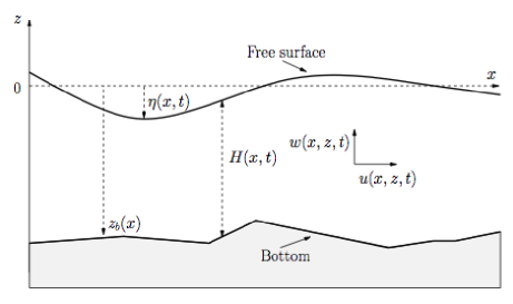
Figure 1: Flow domain with water height $H(x,t)$, free surface $\eta(x,t)$ and bottom $z_{b}(x)$.

As in Ref. [17], we introduce the indicator function for the fluid region

$$\varphi(x,z,t)=\left\{\begin{array}[]{ll}1&\hbox{ for }(x,z)\in\Omega=\{(x,z)\,|\,z_{b}\leq z\leq\eta\},\\ 0&\hbox{ otherwise.}\end{array}\right.$$ (4)

The fluid region is advected by the flow, which can be expressed, thanks to the incompressibility condition, by the relation

$$\frac{\partial\varphi}{\partial t}+\frac{\partial\varphi u}{\partial x}+\frac{\partial\varphi w}{\partial z}=0.$$ (5)

The solution $\varphi$ of this equation takes the values 0 and 1 only but it needs not be of the form (4) at all times. The analysis below is limited to the conditions where this form is preserved. For a more complete presentation of the Navier-Stokes system and its closure, the reader can refer to [21].

Remark 2.1

Notice that in the fluid domain, Eq. (5) reduces to the divergence free condition whereas across the upper and lower boundaries it gives the kinematic boundary conditions defined in the following.

2.2 Boundary conditions

The system (1)-(3) is completed with boundary conditions. We not consider here lateral boundary conditions that can be usual usual inflow and outflow boundary conditions. The outward unit normal vector to the free surface ${\bf n}_{s}$ and the upward unit normal vector to the bottom ${\bf n}_{b}$ are given by

$${\bf n}_{s}=\frac{1}{\sqrt{1+\bigl{(}\frac{\partial\eta}{\partial x}\bigr{)}^{2}}}\left(\begin{array}[]{c}-\frac{\partial\eta}{\partial x}\\ 1\end{array}\right),\quad{\bf n}_{b}=\frac{1}{\sqrt{1+\bigl{(}\frac{\partial z_{b}}{\partial x}\bigr{)}^{2}}}\left(\begin{array}[]{c}-\frac{\partial z_{b}}{\partial x}\\ 1\end{array}\right)\equiv\left(\begin{array}[]{c}-s_{b}\\ c_{b}\end{array}\right),$$

respectively. We use here the same definition for $s_{b}(x)$ and $c_{b}(x)$ as in [9], $c_{b}(x)>0$ is the cosine of the angle between ${\bf n}_{b}$ and the vertical.

2.2.1 Free surface conditions

At the free surface we have the kinematic boundary condition

$$\frac{\partial\eta}{\partial t}+u_{s}\frac{\partial\eta}{\partial x}-w_{s}=0,$$ (6)

where the subscript $s$ indicates the value of the considered quantity at the free surface.

Assuming negligible the air viscosity, the continuity of stresses at the free boundary imposes

$$\Sigma_{T}{\bf n}_{s}=-p^{a}{\bf n}_{s},$$ (7)

where $p^{a}=p^{a}(x,t)$ is a given function corresponding to the atmospheric pressure. Within this paper, we consider $p^{a}=0$.

2.2.2 Bottom conditions

The kinematic boundary condition at the bottom consists in a classical no-penetration condition:

$${\bf u}_{b}\cdot{\bf n}_{b}=0,\quad\mbox{or}\quad u_{b}\frac{\partial z_{b}}{\partial x}-w_{b}=0.$$ (8)

For the stresses at the bottom we consider a wall law under the form

$$\Sigma_{T}{\bf n}_{b}-({\bf n}_{b}\cdot\Sigma_{T}{\bf n}_{b}){\bf n}_{b}=\kappa{\bf u_{b}}$$ (9)

and for ${\bf t}_{b}=^{t}\!\!(c_{b},s_{b})$, using (8) we have

$${\bf t}_{b}\cdot\Sigma_{T}{\bf n}_{b}=\frac{\kappa}{c_{b}}u_{b},$$ (10)

If $\kappa({\bf u_{b}},H)$ is constant then we recover a Navier friction condition as in [17]. Introducing a laminar friction $k_{l}$ and a turbulent friction $k_{t}$, we use the expression

$$\kappa({\bf u_{b}},H)=k_{l}+k_{t}H|{\bf u_{b}}|,$$

corresponding to the boundary condition used in [22]. Another form of $\kappa({\bf u_{b}},H)$ is used in [9], and for other wall laws the reader can also refer to [24]. Due to thermo-mechanical considerations, in the sequel we will suppose $\kappa({\bf u_{b}},H)\geq 0$, and $\kappa({\bf u_{b}},H)$ will be often simply denoted by $\kappa$.

2.3 Other writing

For reasons that will appear later, we rewrite (1)-(3) under the form

$$\frac{\partial u}{\partial x}+\frac{\partial w}{\partial z}=0,$$ (11)

$$\frac{\partial u}{\partial t}+\frac{\partial u^{2}}{\partial x}+\frac{\partial uw}{\partial z}+g\frac{\partial\eta}{\partial x}=\frac{\partial\Sigma_{xx}}{\partial x}+\frac{\partial\Sigma_{xz}}{\partial z}+\frac{\partial^{2}}{\partial x^{2}}\int_{z}^{\eta}\Sigma_{zx}dz_{1}-\frac{\partial\Sigma_{zz}}{\partial x},$$ (12)

where Eq. (12) has been obtained as follows. Integrating Eq. (3) from $z$ to $\eta$ and taking into account the boundary condition (7) gives

$$p=g(\eta-z)-\frac{\partial}{\partial x}\int_{z}^{\eta}\Sigma_{zx}dz_{1}+\Sigma_{zz}.$$ (13)

Inserting the previous expression for $p$ in Eq. (2) gives Eq. (12).

2.4 Energy balance

Lemma 2.2

We recall the fundamental stability property related to the fact that the hydrostatic Navier-Stokes system admits an energy that can be written under the form

$$\frac{\partial}{\partial t}\int_{z_{b}}^{\eta}E\ dz+\frac{\partial}{\partial x}\int_{z_{b}}^{\eta}\Bigl{[}u\Bigl{(}E+g(\eta-z)-(\Sigma_{xx}-\Sigma_{zz})-\frac{\partial}{\partial x}\int_{z}^{\eta}\Sigma_{zx}dz_{1}\Bigr{)}-w\Sigma_{zx}\Bigr{]}dz\\ =-\int_{z_{b}}^{\eta}\Bigl{(}\frac{\partial u}{\partial x}(\Sigma_{xx}-\Sigma_{zz})+\frac{\partial u}{\partial z}\Sigma_{xz}+\frac{\partial w}{\partial x}\Sigma_{zx}\Bigr{)}dz-\frac{\kappa}{c_{b}^{3}}u_{b}^{2},$$ (14)

with

$$E=\frac{u^{2}}{2}+gz.$$ (15)

The way the energy balance (14) is obtained is classical. Considering smooth solutions, first we multiply Eq. (2) by $u$ and Eq. (3) by $w$ then we sum the two obtained equations. After simple manipulations and using the kinematic and dynamic boundary conditions (6)-(9), we obtain the relation

$$\frac{\partial}{\partial t}\int_{z_{b}}^{\eta}E\ dz+\frac{\partial}{\partial x}\int_{z_{b}}^{\eta}\Bigl{[}u\bigl{(}E+p\bigr{)}-u\Sigma_{xx}-w\Sigma_{zx}\Bigr{]}dz\\ =-\int_{z_{b}}^{\eta}\Sigma_{xx}\frac{\partial u}{\partial x}dz-\int_{z_{b}}^{\eta}\Sigma_{xz}\frac{\partial u}{\partial z}dz-\int_{z_{b}}^{\eta}\frac{\partial w}{\partial x}\Sigma_{zx}dz-\int_{z_{b}}^{\eta}\Sigma_{zz}\frac{\partial w}{\partial z}dz-\frac{\kappa}{c_{b}^{3}}u_{b}^{2}.$$

By using Eq. (1) and replacing $p$ by its expression given by (13) in the previous relation gives the result.

$\blacksquare$

3 Depth-averaged solutions of the Euler system

In this section, neglecting the viscous effects in Eqs. (1)-(3), we consider the free surface hydrostatic Euler equations written in a conservative form

$$\frac{\partial\varphi}{\partial t}+\frac{\partial\varphi u}{\partial x}+\frac{\partial\varphi w}{\partial z}=0,$$ (16)

$$\frac{\partial\varphi u}{\partial t}+\frac{\partial\varphi u^{2}}{\partial x}+\frac{\partial\varphi uw}{\partial z}+\frac{\partial p}{\partial x}=0,$$ (17)

$$\hskip 85.35826pt\frac{\partial p}{\partial z}=-\varphi g,$$ (18)

with $\varphi$ defined by (4). This system is completed with the boundary conditions (6),(8) and (7) that reduces to

$$p_{s}=0.$$ (19)

From Eqs. (18),(19), we get

$$p=\varphi g(\eta-z).$$ (20)

The energy balance associated with the hydrostatic Euler system is given by

$$\frac{\partial}{\partial t}\int_{z_{b}}^{\eta}E\ dz+\frac{\partial}{\partial x}\int_{z_{b}}^{\eta}u\bigl{(}E+p\bigr{)}dz=0,$$ (21)

with $E$ defined by (15).

3.1 Vertical discretization of the fluid domain

The interval $[z_{b},\eta]$ is divided into $N$ layers $\{L_{\alpha}\}_{\alpha\in\{1,\ldots,N\}}$ of thickness $l_{\alpha}H(x,t)$ where each layer $L_{\alpha}$ corresponds to the points satisfying $z\in L_{\alpha}(x,t)=]z_{\alpha-1/2},z_{\alpha+1/2}[$ with

$$\left\{\begin{array}[]{l}z_{\alpha+1/2}(x,t)=z_{b}(x)+\sum_{j=1}^{\alpha}l_{j}H(x,t),\\ h_{\alpha}(x,t)=z_{\alpha+1/2}(x,t)-z_{\alpha-1/2}(x,t)=l_{\alpha}H(x,t),\quad\alpha\in\{1,\ldots,N\},\end{array}\right.$$ (22)

with $l_{j}>0,\quad\sum_{j=1}^{N}l_{j}=1$, see Fig. 2.

We also define

$$z_{\alpha}=\frac{z_{\alpha+1/2}+z_{\alpha-1/2}}{2}=z_{\alpha-1/2}+\frac{h_{\alpha}}{2},\quad\alpha=\{1,\ldots,N\}.$$ (23)

We finally introduced the distance between the midpoints of the layers,

$$h_{\alpha+1/2}=z_{\alpha+1}-z_{\alpha}=\frac{h_{\alpha+1}+h_{\alpha}}{2},\quad\alpha=\{1,\ldots,N-1\}.$$ (24)

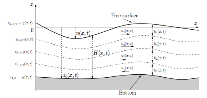
Figure 2: Notations for the multilayer approach.

3.2 Layer-averaging of the Euler solution

In this section we take the vertical average of the Euler system and study the necessary closure relations for this system.

Let us denote $\langle{f}\rangle_{\alpha}$ the integral along the vertical axis in the layer $\alpha$ of the quantity $f=f(z)$ i.e.

$$\langle{f}\rangle_{\alpha}(x,t)=\int_{\mathbb{R}}f(x,z,t){\bf 1}_{z\in L_{\alpha}(x,t)}dz,$$ (25)

where ${\bf 1}_{z\in L_{\alpha}(x,t)}(z)$ is the characteristic function of the layer $\alpha$.

The goal is to propose a new derivation of the so-called multilayer model with mass exchanges [6, 5] using the entropy-based moment closures proposed by Levermore in [19] for kinetic equations. This method has already been successfully used by some of the authors in [11].

Taking into account the kinematic boundary conditions (6) and (8), the layer-averaged form of the Euler system (16)–(18) writes

$$\frac{\partial}{\partial t}\langle{\varphi}\rangle_{\alpha}+\frac{\partial}{\partial x}\langle{\varphi u}\rangle_{\alpha}=G_{\alpha+1/2}-G_{\alpha-1/2},$$ (26)

$$\frac{\partial}{\partial t}\langle{\varphi u}\rangle_{\alpha}+\frac{\partial}{\partial x}\langle{\varphi u^{2}}\rangle_{\alpha}+\langle{\frac{\partial p}{\partial x}}\rangle_{\alpha}=u_{\alpha+1/2}G_{\alpha+1/2}-u_{\alpha-1/2}G_{\alpha-1/2},$$ (27)

$$\langle{\frac{\partial p}{\partial z}}\rangle_{\alpha}=-\langle{\varphi g}\rangle_{\alpha},$$ (28)

$$\frac{\partial}{\partial t}\langle{\varphi z}\rangle_{\alpha}+\frac{\partial}{\partial x}\langle{\varphi zu}\rangle_{\alpha}=\langle{\varphi w}\rangle_{\alpha}+z_{\alpha+1/2}G_{\alpha+1/2}-z_{\alpha-1/2}G_{\alpha-1/2},$$ (29)

for $\alpha\in\{1,\ldots,N\}$ and where $p$ is defined by Eq. (20). The quantity $G_{\alpha+1/2}$ is defined by

$$G_{\alpha+1/2}=\varphi_{\alpha+1/2}\left(\frac{\partial z_{\alpha+1/2}}{\partial t}+u_{\alpha+1/2}\frac{\partial z_{\alpha+1/2}}{\partial x}-w_{\alpha+1/2}\right),$$ (30)

and corresponds to the mass flux leaving/entering the layer $\alpha$ through the interface $z_{\alpha+1/2}$. The value of $\varphi_{\alpha+1/2}$ is equal to 1 for every $\alpha$. Notice that the kinematic boundary conditions (6) and (8) can be written

$$G_{1/2}=0,\quad G_{N+1/2}=0.$$ (31)

These equations just express that there is no loss/supply of mass through the bottom and the free surface. Taking into account the condition (31), the sum for $j=1,\ldots\alpha$ of the relations (26) gives

$$G_{\alpha+1/2}=\frac{\partial}{\partial t}\sum_{j=1}^{\alpha}\langle{\varphi}\rangle_{j}+\frac{\partial}{\partial x}\sum_{j=1}^{\alpha}\langle{\varphi u}\rangle_{j}.$$ (32)

The quantities

$$u_{\alpha+1/2}=u(x,z_{\alpha+1/2},t),$$ (33)

corresponding to the velocities values on the interfaces will be defined later. Notice that when using the expression (32), the velocities $w_{\alpha+1/2}$ no more appear in Eqs. (26)-(29) and thus need not be defined.

Equation (29) is a rewriting of

$$\langle{\int_{z_{\alpha-1/2}}^{z}\left(\frac{\partial{\varphi}}{\partial{t}}+\frac{\partial{\varphi u}}{\partial{x}}+\frac{\partial{\varphi w}}{\partial{z}}\right)dz}\rangle_{\alpha}=\langle{z\left(\frac{\partial{\varphi}}{\partial{t}}+\frac{\partial{\varphi u}}{\partial{x}}+\frac{\partial{\varphi w}}{\partial{z}}\right)}\rangle_{\alpha}=0,$$

using again the kinematic boundary conditions. Notice also that because of the hydrostatic assumption, Eq. (29) is not a kinematic constraint over the velocity field but the definition of the vertical velocity $\langle{\varphi w}\rangle_{\alpha}$. The form of Eq. (29) is useful to derive energy balances but other equivalent writings can be used, see paragraph 4.2.

Simple manipulations allow to obtain the system (26)-(30) from the Euler system (16)-(18) with (6) and (8) e.g. for Eq. (26), starting from (16) we write

$$\langle{\frac{\partial\varphi}{\partial t}+\frac{\partial\varphi u}{\partial x}+\frac{\partial\varphi w}{\partial z}}\rangle_{\alpha}=0,$$

and using the Leibniz rule to permute the derivative and the integral directly gives (26). Likewise, the Leibniz rule written for the pressure $p$ gives

$$\langle{\frac{\partial p}{\partial x}}\rangle_{\alpha}=\int_{z_{\alpha-1/2}}^{z_{\alpha+1/2}}\frac{\partial p}{\partial x}dz=\frac{\partial}{\partial x}\langle{p}\rangle_{\alpha}-p_{\alpha+1/2}\frac{\partial z_{\alpha+1/2}}{\partial x}+p_{\alpha-1/2}\frac{\partial z_{\alpha-1/2}}{\partial x},$$

and from (28),(19), we get

$$p_{\alpha+1/2}=p(x,z_{\alpha+1/2},t)=\sum_{j=\alpha+1}^{N}\langle{\varphi g}\rangle_{j}.$$ (34)

From Eq. (20), we also have

$$\langle{\frac{\partial p}{\partial x}}\rangle_{\alpha}=\int_{z_{\alpha-1/2}}^{z_{\alpha+1/2}}g\frac{\partial}{\partial x}\bigl{(}\varphi(\eta-z)\bigr{)}dz=\frac{\partial}{\partial x}\Bigl{(}\frac{g}{2}\langle{\varphi}\rangle_{\alpha}H\Bigr{)}+g\langle{\varphi}\rangle_{\alpha}\frac{\partial z_{b}}{\partial x}.$$

Relation (20) also leads to

$$p=p_{\alpha+1/2}+g\varphi(z_{\alpha+1/2}-z)=p_{\alpha-1/2}+g\varphi(z_{\alpha-1/2}-z),$$

and hence

$$\langle{p}\rangle_{\alpha}=\langle{\varphi}\rangle_{\alpha}\frac{p_{\alpha+1/2}+p_{\alpha-1/2}}{2}=\langle{\varphi}\rangle_{\alpha}p_{\alpha+1/2}+\frac{g}{2}\langle{\varphi}\rangle_{\alpha}^{2}.$$ (35)

Therefore, the system (26)-(30) can be rewritten under the form

$$\frac{\partial}{\partial t}\langle{\varphi}\rangle_{\alpha}+\frac{\partial}{\partial x}\langle{\varphi u}\rangle_{\alpha}=G_{\alpha+1/2}-G_{\alpha-1/2},$$ (36)

$$\frac{\partial}{\partial t}\langle{\varphi u}\rangle_{\alpha}+\frac{\partial}{\partial x}\left(\langle{\varphi u^{2}}\rangle_{\alpha}+\langle{p}\rangle_{\alpha}\right)=u_{\alpha+1/2}G_{\alpha+1/2}-u_{\alpha-1/2}G_{\alpha-1/2}$$

$$\hskip 170.71652pt+p_{\alpha+1/2}\frac{\partial z_{\alpha+1/2}}{\partial x}-p_{\alpha-1/2}\frac{\partial z_{\alpha-1/2}}{\partial x},$$ (37)

$$\frac{\partial}{\partial t}\langle{\varphi z}\rangle_{\alpha}+\frac{\partial}{\partial x}\langle{\varphi zu}\rangle_{\alpha}=\langle{\varphi w}\rangle_{\alpha}+z_{\alpha+1/2}G_{\alpha+1/2}-z_{\alpha-1/2}G_{\alpha-1/2},$$ (38)

with (34),(35) and completed with relations (32).

Considering smooth solutions, multiplying (17) by $u$ and integrating it over the layer $\alpha$ gives, after simple manipulations, the energy balance

$$\frac{\partial}{\partial t}\langle{E}\rangle_{\alpha}+\frac{\partial}{\partial x}\langle{u(E+p)}\rangle_{\alpha}=\left(\frac{u_{\alpha+1/2}^{2}}{2}+p_{\alpha+1/2}+gz_{\alpha+1/2}\right)G_{\alpha+1/2}\\ -\left(\frac{u_{\alpha-1/2}^{2}}{2}+p_{\alpha-1/2}+gz_{\alpha-1/2}\right)G_{\alpha-1/2}-p_{\alpha+1/2}\frac{\partial z_{\alpha+1/2}}{\partial t}+p_{\alpha-1/2}\frac{\partial z_{\alpha-1/2}}{\partial t},$$ (39)

where $E=E(z;u)$ is defined by (15). The sum for $\alpha=1,\ldots,N$ of the relations (39) gives

$$\frac{\partial}{\partial t}\sum_{\alpha=1}^{N}\langle{E}\rangle_{\alpha}+\frac{\partial}{\partial x}\sum_{\alpha=1}^{N}\langle{u(E+p)}\rangle_{\alpha}=0.$$

Therefore the system (36)-(38) completed (32), (34) and (35) has three equations with three unknowns, namely $\langle{\varphi}\rangle_{\alpha}$, $\langle{\varphi u}\rangle_{\alpha}$ and $\langle{\varphi w}\rangle_{\alpha}$ and closure relations are needed to define $\langle{\varphi u^{2}}\rangle_{\alpha}$, $\langle{\varphi zu}\rangle_{\alpha}$ and $u(x,z_{\alpha+1/2},t)$.

3.3 Closure relations

If $u^{\prime}_{\alpha}$ is defined as the deviation of $u$ with respect to its layer-average over the layer $\alpha$, then it comes for $z\in L_{\alpha}$

$$\varphi u=\frac{\langle{\varphi u}\rangle_{\alpha}}{\langle{\varphi}\rangle_{\alpha}}+\varphi u^{\prime}_{\alpha},$$ (40)

with $\langle{\varphi u^{\prime}_{\alpha}}\rangle=0$. Following the moment closure proposed by Levermore [19], we study the minimization problem

$$\min_{u^{\prime}_{\alpha}}\langle{\{\varphi E(z;u)\}}\rangle_{\alpha}.$$ (41)

The energy $E(z;u)$ being quadratic with respect to $u$ we notice that

$$\langle{\varphi u^{2}}\rangle_{\alpha} = \frac{\langle{\varphi u}\rangle^{2}_{\alpha}}{\langle{\varphi}\rangle_{\alpha}}+\frac{2\langle{\varphi uu^{\prime}}\rangle_{\alpha}}{\langle{\varphi}\rangle_{\alpha}}+\langle{\varphi(u^{\prime}_{\alpha})^{2}}\rangle_{\alpha}$$ (42)

$$= \frac{\langle{\varphi u}\rangle^{2}_{\alpha}}{\langle{\varphi}\rangle_{\alpha}}+\langle{\varphi(u^{\prime}_{\alpha})^{2}}\rangle_{\alpha}$$

$$\geq \frac{\langle{\varphi u}\rangle^{2}_{\alpha}}{\langle{\varphi}\rangle_{\alpha}}.$$

Equation (42) means that the solution of the minimization problem (41) is given by

$$\langle{\varphi E\left(z;\frac{\langle{\varphi u}\rangle_{\alpha}}{\langle{\varphi}\rangle_{\alpha}}\right)}\rangle_{\alpha}=\min_{u^{\prime}_{\alpha}}\langle{\{\varphi E(z;u)\}}\rangle_{\alpha}.$$ (43)

and

$$\langle{\varphi E\left(z;\frac{\langle{\varphi u}\rangle_{\alpha}}{\langle{\varphi}\rangle_{\alpha}}\right)}\rangle_{\alpha}=\frac{\langle{\varphi u}\rangle^{2}_{\alpha}}{2\langle{\varphi}\rangle_{\alpha}}+g\langle{\varphi z}\rangle_{\alpha}.$$ (44)

Since the only choice leading to an equality in relation (42) corresponds to

$$\varphi u=\frac{\langle{\varphi u}\rangle_{\alpha}}{\langle{\varphi}\rangle_{\alpha}},\quad\mbox{for }z\in L_{\alpha},$$ (45)

this allows to precise the closure relation associated to a minimal energy, namely

$$\langle{\varphi u^{2}}\rangle_{\alpha}=\frac{\langle{\varphi u}\rangle_{\alpha}^{2}}{\langle{\varphi}\rangle_{\alpha}},$$ (46)

$$\langle{\varphi zu}\rangle_{\alpha}=\langle{\varphi z}\rangle_{\alpha}\frac{\langle{\varphi u}\rangle_{\alpha}}{\langle{\varphi}\rangle_{\alpha}}.$$ (47)

It remains to define the quantities $u_{\alpha+1/2}$. We adopt the definition

$$u_{\alpha+1/2}=\left\{\begin{array}[]{ll}\frac{\langle{\varphi u}\rangle_{\alpha}}{\langle{\varphi}\rangle_{\alpha}}&\mbox{if }\;G_{\alpha+1/2}\leq 0\\ \frac{\langle{\varphi u}\rangle_{\alpha+1}}{\langle{\varphi}\rangle_{\alpha+1}}&\mbox{if }\;G_{\alpha+1/2}>0\end{array}\right.$$ (48)

corresponding to an upwind definition, depending on the mass exchange sign between the layers $\alpha$ and $\alpha+1$. This choice is justified by the form of energy balance in the following proposition.

Proposition 3.1

The solutions of the Euler system (16)-(18) with (6),(8) satisfying the closure relations (46)-(48) are also solutions of the system

$$\frac{\partial}{\partial t}\langle{\varphi}\rangle_{\alpha}+\frac{\partial}{\partial x}\langle{\varphi u}\rangle_{\alpha}=G_{\alpha+1/2}-G_{\alpha-1/2},$$ (49)

$$\frac{\partial}{\partial t}\langle{\varphi u}\rangle_{\alpha}+\frac{\partial}{\partial x}\left(\frac{\langle{\varphi u}\rangle_{\alpha}^{2}}{\langle{\varphi}\rangle_{\alpha}}+\langle{p}\rangle_{\alpha}\right)=u_{\alpha+1/2}G_{\alpha+1/2}-u_{\alpha-1/2}G_{\alpha-1/2}$$

$$\hskip 170.71652pt+p_{\alpha+1/2}\frac{\partial z_{\alpha+1/2}}{\partial x}-p_{\alpha-1/2}\frac{\partial z_{\alpha-1/2}}{\partial x},$$ (50)

$$\frac{\partial}{\partial t}\langle{\varphi z}\rangle_{\alpha}+\frac{\partial}{\partial x}\left(\langle{\varphi z}\rangle_{\alpha}\frac{\langle{\varphi u}\rangle_{\alpha}}{\langle{\varphi}\rangle_{\alpha}}\right)=\langle{\varphi w}\rangle_{\alpha}+z_{\alpha+1/2}G_{\alpha+1/2}-z_{\alpha-1/2}G_{\alpha-1/2},$$ (51)

completed with relation (32). The quantities $\langle{p}\rangle_{\alpha}$ and $p_{\alpha+1/2}$ are defined by (34) and (35).

This system is a layer-averaged approximation of the Euler system and admits – for smooth solutions – an energy equality under the form

$$\frac{\partial}{\partial t}\sum_{\alpha=1}^{N}\langle{E\left(z;\frac{\langle{\varphi u}\rangle_{\alpha}}{\langle{\varphi}\rangle_{\alpha}}\right)}\rangle_{\alpha}+\frac{\partial}{\partial x}\sum_{\alpha=1}^{N}\langle{\frac{\langle{\varphi u}\rangle_{\alpha}}{\langle{\varphi}\rangle_{\alpha}}\left(E\left(z;\frac{\langle{\varphi u}\rangle_{\alpha}}{\langle{\varphi}\rangle_{\alpha}}\right)+\langle{p}\rangle_{\alpha}\right)}\rangle_{\alpha}=\\ -\frac{1}{2}\sum_{\alpha=1}^{N}\left(\frac{\langle{\varphi u}\rangle_{\alpha+1}}{\langle{\varphi}\rangle_{\alpha+1}}-\frac{\langle{\varphi u}\rangle_{\alpha}}{\langle{\varphi}\rangle_{\alpha}}\right)^{2}|G_{\alpha+1/2}|.$$ (52)

Remark 3.2

Instead of (48), the definition

$$u_{\alpha+1/2}=\frac{1}{2}\left(\frac{\langle{\varphi u}\rangle_{\alpha+1}}{\langle{\varphi}\rangle_{\alpha+1}}+\frac{\langle{\varphi u}\rangle_{\alpha}}{\langle{\varphi}\rangle_{\alpha}}\right),$$ (53)

is also possible and gives a vanishing right hand side in (52). But such a choice does not allow to obtain an energy balance in the variable density case and does not give a maximum principle, at the discrete level, see [5]. Simple calculations show that any other choice that (48) or (53) leads to a non negative r.h.s. in (52), see Eq. (54) in the proof of prop. 52.

Remark 3.3

It is important to notice that whereas the solution $H,u,w,p$ of the Euler system (16)-(19),(6),(8) also satisfies the system (36)-(38), only the solutions $H,u,w,p$ of the Euler system (16)-(19),(6),(8) satisfying the closure relations (46)-(47),(48) are also solutions of the system (49)-(52). On the contrary, any solutions $\langle{\varphi}\rangle_{\alpha}$, $\langle{\varphi u}\rangle_{\alpha}$, $\langle{\varphi w}\rangle_{\alpha}$ and $\langle{p}\rangle_{\alpha}$ of (49)-(51) with (48) are also solutions of (36)-(39).

• Only the manipulations allowing to obtain (52) have to be detailed. For that purpose, we multiply (50) by $\frac{\langle{\varphi u}\rangle_{\alpha}}{\langle{\varphi}\rangle_{\alpha}}$ giving

  $$\left(\frac{\partial}{\partial t}\frac{\langle{\varphi u}\rangle_{\alpha}}{\langle{\varphi}\rangle_{\alpha}}+\frac{\partial}{\partial x}\left(\frac{\langle{\varphi u}\rangle_{\alpha}^{2}}{\langle{\varphi}\rangle_{\alpha}}+\langle{p}\rangle_{\alpha}\right)\right)\frac{\langle{\varphi u}\rangle_{\alpha}}{\langle{\varphi}\rangle_{\alpha}}=\biggl{(}u_{\alpha+1/2}G_{\alpha+1/2}-u_{\alpha-1/2}G_{\alpha-1/2}\\ +\frac{\partial z_{\alpha+1/2}}{\partial x}p_{\alpha+1/2}-\frac{\partial z_{\alpha-1/2}}{\partial x}p_{\alpha-1/2}\biggr{)}\frac{\langle{\varphi u}\rangle_{\alpha}}{\langle{\varphi}\rangle_{\alpha}},$$

  and we rewrite each of the obtained terms.

  Considering first the left hand side of the preceding equation excluding the pressure terms, we denote

  $$I_{u,\alpha}=\left(\frac{\partial}{\partial t}\frac{\langle{\varphi u}\rangle_{\alpha}}{\langle{\varphi}\rangle_{\alpha}}+\frac{\partial}{\partial x}\left(\frac{\langle{\varphi u}\rangle_{\alpha}^{2}}{\langle{\varphi}\rangle_{\alpha}}\right)\right)\frac{\langle{\varphi u}\rangle_{\alpha}}{\langle{\varphi}\rangle_{\alpha}},$$

  and using (26) we have

  $$I_{u,\alpha}=\frac{\partial}{\partial t}\left(\frac{\langle{\varphi u}\rangle_{\alpha}^{2}}{2\langle{\varphi}\rangle_{\alpha}}\right)+\frac{\partial}{\partial x}\left(\frac{\langle{\varphi u}\rangle_{\alpha}}{\langle{\varphi}\rangle_{\alpha}}\frac{\langle{\varphi u}\rangle_{\alpha}^{2}}{2\langle{\varphi}\rangle_{\alpha}}\right)+\frac{\langle{\varphi u}\rangle_{\alpha}^{2}}{2\langle{\varphi}\rangle_{\alpha}^{2}}\left(G_{\alpha+1/2}-G_{\alpha-1/2}\right).$$

  Now we consider the contribution of the pressure terms over the energy balance i.e.

  $$I_{p,\alpha}=\left(\frac{\partial\langle{p}\rangle_{\alpha}}{\partial x}-p_{\alpha+1/2}\frac{\partial z_{\alpha+1/2}}{\partial x}+p_{\alpha-1/2}\frac{\partial z_{\alpha-1/2}}{\partial x}\right)\frac{\langle{\varphi u}\rangle_{\alpha}}{\langle{\varphi}\rangle_{\alpha}}.$$

  Using (35) we get the equality

  $$p_{\alpha+1/2}\frac{\partial z_{\alpha+1/2}}{\partial x}-p_{\alpha-1/2}\frac{\partial z_{\alpha-1/2}}{\partial x}=\frac{\langle{p}\rangle_{\alpha}}{\langle{\varphi}\rangle_{\alpha}}\frac{\partial h_{\alpha}}{\partial x}-\langle{g\varphi}\rangle_{\alpha}\frac{\partial z_{\alpha}}{\partial x},$$

  holds, it comes

  $$I_{p,\alpha} = \frac{\partial}{\partial x}\left(\langle{p}\rangle_{\alpha}\frac{\langle{\varphi u}\rangle_{\alpha}}{\langle{\varphi}\rangle_{\alpha}}\right)-\langle{p}\rangle_{\alpha}\frac{\partial}{\partial x}\left(\frac{\langle{\varphi u}\rangle_{\alpha}}{\langle{\varphi}\rangle_{\alpha}}\right)-\frac{\langle{p}\rangle_{\alpha}}{\langle{\varphi}\rangle_{\alpha}}\frac{\langle{\varphi u}\rangle_{\alpha}}{\langle{\varphi}\rangle_{\alpha}}\frac{\partial\langle{\varphi}\rangle_{\alpha}}{\partial x}+g\langle{\varphi u}\rangle_{\alpha}\frac{\partial z_{\alpha}}{\partial x}$$

  $$= \frac{\partial}{\partial x}\left(\langle{p}\rangle_{\alpha}\frac{\langle{\varphi u}\rangle_{\alpha}}{\langle{\varphi}\rangle_{\alpha}}\right)-\frac{\langle{p}\rangle_{\alpha}}{\langle{\varphi}\rangle_{\alpha}}\frac{\partial\langle{\varphi u}\rangle_{\alpha}}{\partial x}+\frac{\partial}{\partial x}\left(gh_{\alpha}z_{\alpha}\frac{\langle{\varphi u}\rangle_{\alpha}}{\langle{\varphi}\rangle_{\alpha}}\right)-z_{\alpha}\frac{\partial}{\partial x}\left(g\langle{\varphi u}\rangle_{\alpha}\right)$$

  $$= \frac{\partial}{\partial x}\left(\langle{p}\rangle_{\alpha}\frac{\langle{\varphi u}\rangle_{\alpha}}{\langle{\varphi}\rangle_{\alpha}}\right)-\frac{\langle{p}\rangle_{\alpha}}{\langle{\varphi}\rangle_{\alpha}}\frac{\partial\langle{\varphi u}\rangle_{\alpha}}{\partial x}+\frac{\partial}{\partial x}\left(gh_{\alpha}z_{\alpha}\frac{\langle{\varphi u}\rangle_{\alpha}}{\langle{\varphi}\rangle_{\alpha}}\right)+z_{\alpha}\frac{\partial}{\partial t}\left(\langle{g\varphi}\rangle_{\alpha}\right)$$

  $$-gz_{\alpha}\left(G_{\alpha+1/2}-G_{\alpha-1/2}\right)$$

  $$= \frac{\partial}{\partial x}\left(\langle{p}\rangle_{\alpha}\frac{\langle{\varphi u}\rangle_{\alpha}}{\langle{\varphi}\rangle_{\alpha}}\right)-\frac{\langle{p}\rangle_{\alpha}}{\langle{\varphi}\rangle_{\alpha}}\frac{\partial\langle{\varphi u}\rangle_{\alpha}}{\partial x}+\frac{\partial}{\partial x}\left(gh_{\alpha}z_{\alpha}\frac{\langle{\varphi u}\rangle_{\alpha}}{\langle{\varphi}\rangle_{\alpha}}\right)+\frac{\partial}{\partial t}\left(gh_{\alpha}z_{\alpha}\right)$$

  $$-gh_{\alpha}\frac{\partial z_{\alpha}}{\partial t}-gz_{\alpha}\left(G_{\alpha+1/2}-G_{\alpha-1/2}\right).$$

  Let us rewrite $I_{p,\alpha}$ under the form

  $$I_{p,\alpha} = \frac{\partial}{\partial x}\left(\langle{p}\rangle_{\alpha}\frac{\langle{\varphi u}\rangle_{\alpha}}{\langle{\varphi}\rangle_{\alpha}}\right)+\frac{\partial}{\partial t}\left(gh_{\alpha}z_{\alpha}\right)+g\frac{\partial}{\partial x}\left(h_{\alpha}z_{\alpha}\frac{\langle{u}\rangle_{\alpha}}{h_{\alpha}}\right)$$

  $$-g\left(z_{\alpha+1/2}G_{\alpha+1/2}-z_{\alpha-1/2}G_{\alpha-1/2}\right)+J_{p,\alpha},$$

  with

  $$J_{p,\alpha}=-\frac{\langle{p}\rangle_{\alpha}}{\langle{\varphi}\rangle_{\alpha}}\frac{\partial\langle{\varphi u}\rangle_{\alpha}}{\partial x}-gh_{\alpha}\frac{\partial z_{\alpha}}{\partial t}+g\frac{h_{\alpha}}{2}\left(G_{\alpha+1/2}+G_{\alpha-1/2}\right).$$

  Since we have

  $$\frac{\langle{p}\rangle_{\alpha}}{\langle{\varphi}\rangle_{\alpha}}\frac{\partial\langle{\varphi u}\rangle_{\alpha}}{\partial x}=\frac{\langle{\varphi}\rangle_{\alpha}}{\langle{\varphi}\rangle_{\alpha}}\left(G_{\alpha+1/2}-G_{\alpha-1/2}-\frac{\partial h_{\alpha}}{\partial t}\right),$$

  we obtain

  $$J_{p,\alpha} = p_{\alpha+1/2}\frac{\partial z_{\alpha+1/2}}{\partial t}-p_{\alpha-1/2}\frac{\partial z_{\alpha-1/2}}{\partial t}-p_{\alpha+1/2}G_{\alpha+1/2}+p_{\alpha-1/2}G_{\alpha-1/2}.$$

  Then summing $I_{u,\alpha}$ and $I_{p,\alpha}$ gives

  $$\frac{\partial}{\partial t}\langle{E\left(z;\frac{\langle{\varphi u}\rangle_{\alpha}}{\langle{\varphi}\rangle_{\alpha}}\right)}\rangle_{\alpha}+\frac{\partial}{\partial x}\langle{\frac{\langle{\varphi u}\rangle_{\alpha}}{\langle{\varphi}\rangle_{\alpha}}\left(E\left(z;\frac{\langle{\varphi u}\rangle_{\alpha}}{\langle{\varphi}\rangle_{\alpha}}\right)+\langle{p}\rangle_{\alpha}\right)}\rangle_{\alpha}=\\ \left(u_{\alpha+1/2}\frac{\langle{\varphi u}\rangle_{\alpha}}{\langle{\varphi}\rangle_{\alpha}}-\frac{1}{2}\left(\frac{\langle{\varphi u}\rangle_{\alpha}}{\langle{\varphi}\rangle_{\alpha}}\right)^{2}\right)G_{\alpha+1/2}-\left(u_{\alpha-1/2}\frac{\langle{\varphi u}\rangle_{\alpha}}{\langle{\varphi}\rangle_{\alpha}}-\frac{1}{2}\left(\frac{\langle{\varphi u}\rangle_{\alpha}}{\langle{\varphi}\rangle_{\alpha}}\right)^{2}\right)G_{\alpha-1/2}.$$

  Finally, the sum of the preceding relations for $\alpha=1,\ldots,N$

  $$\frac{\partial}{\partial t}\sum_{\alpha=1}^{N}\langle{E\left(z;\frac{\langle{\varphi u}\rangle_{\alpha}}{\langle{\varphi}\rangle_{\alpha}}\right)}\rangle_{\alpha}+\frac{\partial}{\partial x}\sum_{\alpha=1}^{N}\langle{\frac{\langle{\varphi u}\rangle_{\alpha}}{\langle{\varphi}\rangle_{\alpha}}\left(E\left(z;\frac{\langle{\varphi u}\rangle_{\alpha}}{\langle{\varphi}\rangle_{\alpha}}\right)+\langle{p}\rangle_{\alpha}\right)}\rangle_{\alpha}=\\ \sum_{\alpha=1}^{N}\left(u_{\alpha+1/2}\left(\frac{\langle{\varphi u}\rangle_{\alpha}}{\langle{\varphi}\rangle_{\alpha}}-\frac{\langle{\varphi u}\rangle_{\alpha+1}}{\langle{\varphi}\rangle_{\alpha+1}}\right)-\frac{1}{2}\left(\frac{\langle{\varphi u}\rangle_{\alpha}}{\langle{\varphi}\rangle_{\alpha}}\right)^{2}+\frac{1}{2}\left(\frac{\langle{\varphi u}\rangle_{\alpha+1}}{\langle{\varphi}\rangle_{\alpha+1}}\right)^{2}\right)G_{\alpha+1/2},$$ (54)

  and the definition (48) gives relation (52) that completes the proof. Notice that any other choice than (48) or (53) leads to a non negative r.h.s. in (54), see remark 3.2. $\blacksquare$

4 The proposed layer-averaged Euler system

4.1 Formulation

The closure relations (46)-(47) motivate the definition of piecewise constant approximation of the variables $u$ and $w$.

Let us consider the space $\mathbb{P}_{0,H}^{N,t}$ of piecewise constant functions defined by

$$\mathbb{P}_{0,H}^{N,t}=\left\{{\bf 1}_{z\in L_{\alpha}(x,t)}(z),\quad\alpha\in\{1,\ldots,N\}\right\}.$$

Using this formalism, the projection of $u$ and $w$ on $\mathbb{P}_{0,H}^{N,t}$ is a piecewise constant function defined by

$$X^{N}(x,z,\{z_{\alpha}\},t)=\sum_{\alpha=1}^{N}{\bf 1}_{]z_{\alpha-1/2},z_{\alpha+1/2}[}(z)X_{\alpha}(x,t),$$ (55)

for $X\in(u,w)$. In the following, we no more handle variables corresponding to vertical means of the solution of the Euler equations (16)-(18) and we adopt notations inherited from (55).

By analogy with (49)-(51) we consider the following model

$$\sum_{\alpha=1}^{N}\frac{\partial h_{\alpha}}{\partial t}+\sum_{\alpha=1}^{N}\frac{\partial(h_{\alpha}u_{\alpha})}{\partial x}=0,$$ (56)

$$\frac{\partial h_{\alpha}u_{\alpha}}{\partial t}+\frac{\partial}{\partial x}\left(h_{\alpha}u^{2}_{\alpha}+h_{\alpha}p_{\alpha}\right)=u_{\alpha+1/2}G_{\alpha+1/2}-u_{\alpha-1/2}G_{\alpha-1/2}$$

$$\hskip 162.18062pt+\frac{\partial z_{\alpha+1/2}}{\partial x}p_{\alpha+1/2}-\frac{\partial z_{\alpha-1/2}}{\partial x}p_{\alpha-1/2},$$ (57)

$$\frac{\partial}{\partial t}\left(\frac{z_{\alpha+1/2}^{2}-z_{\alpha-1/2}^{2}}{2}\right)+\frac{\partial}{\partial x}\left(\frac{z_{\alpha+1/2}^{2}-z_{\alpha-1/2}^{2}}{2}u_{\alpha}\right)=h_{\alpha}w_{\alpha}$$

$$\hskip 170.71652pt+z_{\alpha+1/2}G_{\alpha+1/2}-z_{\alpha-1/2}G_{\alpha-1/2},$$ (58)

by analogy with (32)

$$G_{\alpha+1/2}=\frac{\partial}{\partial t}\sum_{j=1}^{\alpha}h_{j}+\frac{\partial}{\partial x}\sum_{j=1}^{\alpha}\left(h_{j}u_{j}\right),$$ (59)

and we have $p_{\alpha}$, $p_{\alpha+1/2}$ given by

$$p_{\alpha}=g\left(\frac{h_{\alpha}}{2}+\sum_{j=\alpha+1}^{N}h_{j}\right)\qquad\mbox{\rm and}\qquad p_{\alpha+1/2}=g\sum_{j=\alpha+1}^{N}h_{j}.$$ (60)

The definition of $u_{\alpha+1/2}$ is equivalent to (48) i.e.

$$u_{\alpha+1/2}=\left\{\begin{array}[]{ll}u_{\alpha}&\mbox{if }\;G_{\alpha+1/2}\leq 0\\ u_{\alpha+1}&\mbox{if }\;G_{\alpha+1/2}>0\end{array}\right.$$

The smooth solutions of (56)-(58) satisfy the energy balance

$$\frac{\partial}{\partial t}E_{\alpha}+\frac{\partial}{\partial x}\left(u_{\alpha}\left(E_{\alpha}+h_{\alpha}p_{\alpha}\right)\right)=\left(u_{\alpha+1/2}u_{\alpha}-\frac{u_{\alpha}^{2}}{2}+p_{\alpha+1/2}+gz_{\alpha+1/2}\right)G_{\alpha+1/2}$$

$$\qquad\qquad-\left(u_{\alpha-1/2}u_{\alpha}-\frac{u_{\alpha}^{2}}{2}+p_{\alpha-1/2}+gz_{\alpha-1/2}\right)G_{\alpha-1/2}$$

$$\qquad\qquad-p_{\alpha+1/2}\frac{\partial z_{\alpha+1/2}}{\partial t}+p_{\alpha-1/2}\frac{\partial z_{\alpha-1/2}}{\partial t},$$ (61)

with

$$E_{\alpha}=\frac{h_{\alpha}u_{\alpha}^{2}}{2}+\frac{g}{2}(z_{\alpha+1/2}^{2}-z_{\alpha-1/2}^{2})=h_{\alpha}\biggl{(}\frac{u_{\alpha}^{2}}{2}+gz_{\alpha}\biggr{)}.$$

Adding the preceding relations for $\alpha=1,\ldots,N$, we obtain the global equality

$$\frac{\partial}{\partial t}\left(\sum_{\alpha=1}^{N}E_{\alpha}\right)+\frac{\partial}{\partial x}\left(\sum_{\alpha=1}^{N}u_{\alpha}\left(E_{\alpha}+h_{\alpha}p_{\alpha}\right)\right)=-\sum_{\alpha=1}^{N}\frac{1}{2}(u_{\alpha+1/2}-u_{\alpha})^{2}|G_{\alpha+1/2}|.$$ (62)

Using (60), the pressure terms in (57) can be rewritten under the form

$$\frac{\partial}{\partial x}\left(h_{\alpha}p_{\alpha}\right)-\frac{\partial z_{\alpha+1/2}}{\partial x}p_{\alpha+1/2}+\frac{\partial z_{\alpha-1/2}}{\partial x}p_{\alpha-1/2}=\frac{\partial}{\partial x}\left(\frac{g}{2}Hh_{\alpha}\right)+gh_{\alpha}\frac{\partial z_{b}}{\partial x}.$$ (63)

4.2 The vertical velocity

The equation (58) is a definition of the vertical velocity $w^{N}$ given by (55). The quantities $w_{\alpha}$ are not unknowns of the problem but only output variables. Indeed, once $H$ and $u^{N}$ have been calculated solving (56),(57) with (59), the vertical velocities $w_{\alpha}$ can be determined using (58).

Using simple manipulations, Eq. (58) can be rewritten under several forms. In particular, the following proposition holds

Proposition 4.1

Let us introduce $\hat{w}=\hat{w}(x,z,t)$ defined by

$$\frac{\partial u^{N}}{\partial x}+\frac{\partial\hat{w}}{\partial z}=0,$$ (64)

The quantity $\hat{w}$ is affine in $z$ and discontinuous at each interface $z_{\alpha+1/2}$, $\hat{w}$ can be written:

$$\hat{w}=k_{\alpha}-z\frac{\partial u_{\alpha}}{\partial x},$$ (65)

with $k_{\alpha}=k_{\alpha}(x,t)$ recursively defined by

$$k_{1}=\frac{\partial(z_{b}u_{1})}{\partial x},$$

$$k_{\alpha+1}=k_{\alpha}+\frac{\partial}{\partial x}\bigl{(}z_{\alpha+1/2}(u_{\alpha+1}-u_{\alpha})\bigr{)}.$$

Therefore we have

$$\int_{z_{\alpha-1/2}}^{z_{\alpha+1/2}}\hat{w}dz=h_{\alpha}w_{\alpha},$$ (66)

meaning the quantities $\hat{w}$ is a natural and consistent affine extension of the layer-averaged quantities $w_{\alpha}$ defined by (58). Using (66), an integration along the layer $\alpha$ of (65) gives

$$h_{\alpha}w_{\alpha}=h_{\alpha}k_{\alpha}-\frac{z_{\alpha+1/2}^{2}-z_{\alpha-1/2}^{2}}{2}\frac{\partial u_{\alpha}}{\partial x}=h_{\alpha}\left(k_{\alpha}-z_{\alpha}\frac{\partial u_{\alpha}}{\partial x}\right).$$ (67)

or

$$w_{\alpha}=k_{\alpha}-z_{\alpha}\frac{\partial u_{\alpha}}{\partial x}=\hat{w}(z_{\alpha}).$$ (68)

• A simple integration along $z$ of equation (64) using (8) gives

  $$\hat{w}=-\frac{\partial}{\partial x}\int_{z_{b}}^{z}u^{N}\ dz,$$ (69)

  and therefore, for $z\in L_{1}$ we get

  $$\hat{w}=-\frac{\partial}{\partial x}\int_{z_{b}}^{z}u_{1}\ dz=-\frac{\partial}{\partial x}\bigl{(}(z-z_{b})u_{1}\bigr{)},$$

  i.e.

  $$\hat{w}=\frac{\partial}{\partial x}(z_{b}u_{1})-z\frac{\partial u_{1}}{\partial x}.$$

  For $z\in L_{\alpha}$, relation (69) gives

  $$\hat{w}=-\sum_{j=1}^{\alpha-1}\frac{\partial}{\partial x}(h_{j}u_{j})-\frac{\partial}{\partial x}\bigl{(}(z-z_{\alpha-1/2})u_{\alpha}\bigr{)},$$ (70)

  and we easily obtain

  $$\hat{w}=k_{\alpha}-z\frac{\partial u_{\alpha}}{\partial x}.$$

  Now we intend to prove (66).

  Using the definition (23), relation (58) also writes

  $$h_{\alpha}w_{\alpha}=\frac{\partial}{\partial x}(z_{\alpha}h_{\alpha}u_{\alpha})-z_{\alpha+1/2}\sum_{j=1}^{\alpha}\frac{\partial(h_{j}u_{j})}{\partial x}+z_{\alpha-1/2}\sum_{j=1}^{\alpha-1}\frac{\partial(h_{j}u_{j})}{\partial x},$$

  leading to a new expression governing $w_{\alpha}$ under the form

  $$h_{\alpha}w_{\alpha}=-\frac{h_{\alpha}}{2}\frac{\partial(h_{\alpha}u_{\alpha})}{\partial x}-h_{\alpha}\sum_{j=1}^{\alpha-1}\frac{\partial(h_{j}u_{j})}{\partial x}+h_{\alpha}u_{\alpha}\frac{\partial z_{\alpha}}{\partial x}.$$ (71)

  And from (70), we get

  $$\int_{z_{\alpha-1/2}}^{z_{\alpha+1/2}}\hat{w}dz = -h_{\alpha}\sum_{j=1}^{\alpha-1}\frac{\partial}{\partial x}(h_{j}u_{j})+h_{\alpha}\frac{\partial}{\partial x}\bigl{(}z_{\alpha-1/2}u_{\alpha}\bigr{)}-h_{\alpha}z_{\alpha}\frac{\partial u_{\alpha}}{\partial x}$$

  $$= -h_{\alpha}\sum_{j=1}^{\alpha-1}\frac{\partial}{\partial x}(h_{j}u_{j})-\frac{h_{\alpha}}{2}\frac{\partial}{\partial x}\left(h_{\alpha}u_{\alpha}\right)+h_{\alpha}u_{\alpha}\frac{\partial z_{\alpha}}{\partial x},$$

  corresponding to (71) and proving the result. $\blacksquare$

Using also (63), we are able to rewrite the system (56)-(58) under the form

$$\sum_{\alpha=1}^{N}\frac{\partial h_{\alpha}}{\partial t}+\sum_{\alpha=1}^{N}\frac{\partial(h_{\alpha}u_{\alpha})}{\partial x}=0,$$ (72)

$$\frac{\partial h_{\alpha}u_{\alpha}}{\partial t}+\frac{\partial}{\partial x}\left(h_{\alpha}u^{2}_{\alpha}+\frac{g}{2}h_{\alpha}H\right)=-gh_{\alpha}\frac{\partial z_{b}}{\partial x}+u_{\alpha+1/2}G_{\alpha+1/2}-u_{\alpha-1/2}G_{\alpha-1/2},$$ (73)

$$w_{\alpha}=-\frac{1}{2}\frac{\partial(h_{\alpha}u_{\alpha})}{\partial x}-\sum_{j=1}^{\alpha-1}\frac{\partial(h_{j}u_{j})}{\partial x}+u_{\alpha}\frac{\partial z_{\alpha}}{\partial x}.$$ (74)

5 The Navier-Stokes system

Instead of considering the Euler system, we can also depart from the Navier-Stokes equations to derive a layer-averaged model.

The model derivation is similar to what has been done in Section 3 for the Euler system.

5.1 Layer averaging of the viscous terms

In this paragraph and the both following, the components of the Cauchy stress tensor $\Sigma$ are not specified. It remains to find a layer-averaged formulation for the r.h.s. of Eq. (12), i.e.

$$V_{\alpha}=\int_{z_{\alpha-1/2}}^{z_{\alpha+1/2}}\left(\frac{\partial\Sigma_{xx}}{\partial x}+\frac{\partial\Sigma_{xz}}{\partial z}+\frac{\partial^{2}}{\partial x^{2}}\int_{z}^{\eta}\Sigma_{zx}dz_{1}-\frac{\partial\Sigma_{zz}}{\partial x}\right)dz.$$

We have

$$V_{\alpha} = \frac{\partial}{\partial x}\int_{z_{\alpha-1/2}}^{z_{\alpha+1/2}}\left(\Sigma_{xx}+\frac{\partial}{\partial x}\int_{z}^{\eta}\Sigma_{zx}dz_{1}-\Sigma_{zz}\right)dz$$

$$+\Sigma_{xz}|_{\alpha+1/2}-\frac{\partial z_{\alpha+1/2}}{\partial x}\left.\left(\Sigma_{xx}+\frac{\partial}{\partial x}\int_{z}^{\eta}\Sigma_{zx}dz_{1}-\Sigma_{zz}\right)\right|_{z_{\alpha+1/2}}$$

$$-\Sigma_{xz}|_{\alpha-1/2}+\frac{\partial z_{\alpha-1/2}}{\partial x}\left.\left(\Sigma_{xx}+\frac{\partial}{\partial x}\int_{z}^{\eta}\Sigma_{zx}dz_{1}-\Sigma_{zz}\right)\right|_{z_{\alpha-1/2}}.$$

In the expression $V_{\alpha}$ we have the term

$$\frac{\partial}{\partial x}\int_{z_{\alpha-1/2}}^{z_{\alpha+1/2}} \left(\frac{\partial}{\partial x}\int_{z}^{\eta}\Sigma_{zx}dz_{1}\right)dz$$

$$= \frac{\partial}{\partial x}\Biggl{(}\frac{\partial}{\partial x}\int_{z_{\alpha-1/2}}^{z_{\alpha+1/2}}\int_{z}^{\eta}\Sigma_{zx}dz_{1}dz-\frac{\partial z_{\alpha+1/2}}{\partial x}\int_{z_{\alpha+1/2}}^{\eta}\Sigma_{zx}dz$$

$$+\frac{\partial z_{\alpha-1/2}}{\partial x}\int_{z_{\alpha-1/2}}^{\eta}\Sigma_{zx}dz\Biggr{)}$$

$$= \frac{\partial}{\partial x}\Biggl{(}\frac{\partial}{\partial x}\int_{z_{\alpha-1/2}}^{z_{\alpha+1/2}}z\Sigma_{zx}dz+z_{\alpha+1/2}\frac{\partial}{\partial x}\int_{z_{\alpha+1/2}}^{\eta}\Sigma_{zx}dz$$

$$-z_{\alpha-1/2}\frac{\partial}{\partial x}\int_{z_{\alpha-1/2}}^{\eta}\Sigma_{zx}dz\Biggr{)},$$

and

$$\frac{\partial z_{\alpha+1/2}}{\partial x}\left.\left(\frac{\partial}{\partial x}\int_{z}^{\eta}\Sigma_{zx}dz_{1}\right)\right|_{z_{\alpha+1/2}}=\frac{\partial z_{\alpha+1/2}}{\partial x}\frac{\partial}{\partial x}\int_{z_{\alpha+1/2}}^{\eta}\Sigma_{zx}dz+\left(\frac{\partial z_{\alpha+1/2}}{\partial x}\right)^{2}\Sigma_{zx|_{\alpha+1/2}},$$

$$\frac{\partial z_{\alpha-1/2}}{\partial x}\left.\left(\frac{\partial}{\partial x}\int_{z}^{\eta}\Sigma_{zx}dz_{1}\right)\right|_{z_{\alpha-1/2}}=\frac{\partial z_{\alpha-1/2}}{\partial x}\frac{\partial}{\partial x}\int_{z_{\alpha-1/2}}^{\eta}\Sigma_{zx}dz+\left(\frac{\partial z_{\alpha-1/2}}{\partial x}\right)^{2}\Sigma_{zx|_{\alpha-1/2}}.$$

5.2 Definitions and closure relation

The expression of the viscous terms generally involving second order derivatives, their discretization requires quadrature formula that are not inherited from the layer-averaged discretization. In particular, at this step of the paper, we adopt the following notations

$$\Sigma_{ab|_{\alpha+1/2}}\approx\Sigma_{ab,{\alpha+1/2}}\ ,$$ (75)

and

$$\Sigma_{ab|_{\alpha}}\approx\Sigma_{ab,{\alpha}}\ ,$$ (76)

and the following definitions,

$$\int_{z_{\alpha-1/2}}^{z_{\alpha+1/2}}\Sigma_{ab}dz\approx h_{\alpha}\Sigma_{ab,\alpha}\ ,$$ (77)

with $(a,b)\in(x,z)^{2}$. For the terms having the form

$$\int_{z_{\alpha-1/2}}^{z_{\alpha+1/2}}z\Sigma_{ab}dz,$$

a closure relation is needed and we choose the approximation

$$\int_{z_{\alpha-1/2}}^{z_{\alpha+1/2}}z\Sigma_{ab}dz\approx\frac{z_{\alpha+1/2}^{2}-z_{\alpha-1/2}^{2}}{2}\Sigma_{ab,\alpha}=h_{\alpha}z_{\alpha}\Sigma_{ab,\alpha}.$$ (78)

For each interface $z_{\alpha+1/2}$ we introduce the unit normal vector ${\bf n}_{\alpha+1/2}$ and the unit tangent vector ${\bf t}_{\alpha+1/2}$ given by:

$${\bf n}_{\alpha+1/2}=\frac{1}{\sqrt{1+\bigl{(}\frac{\partial z_{\alpha+1/2}}{\partial x}\bigr{)}^{2}}}\left(\begin{array}[]{c}-\frac{\partial z_{\alpha+1/2}}{\partial x}\\ 1\end{array}\right)\equiv\left(\begin{array}[]{c}-s_{\alpha+1/2}\\ c_{\alpha+1/2}\end{array}\right),\quad{\bf t}_{\alpha+1/2}=\left(\begin{array}[]{c}c_{\alpha+1/2}\\ s_{\alpha+1/2}\end{array}\right).$$

Then, for $0\leqslant\alpha\leqslant N$, we have the following expression

$${\bf t}_{\alpha+1/2}\cdot\Sigma_{\alpha+1/2}{\bf n}_{\alpha+1/2}=\frac{1}{1+\bigl{(}\frac{\partial z_{\alpha+1/2}}{\partial x}\bigr{)}^{2}}\Biggl{(}\Sigma_{xz,\alpha+1/2}\\ -\frac{\partial z_{\alpha+1/2}}{\partial x}\Bigl{(}\Sigma_{xx,\alpha+1/2}+\frac{\partial z_{\alpha+1/2}}{\partial x}\Sigma_{zx,\alpha+1/2}-\Sigma_{zz,\alpha+1/2}\Bigr{)}\biggr{)},$$ (79)

which can be rewritten as

$${\bf t}_{\alpha+1/2}\cdot\Sigma_{\alpha+1/2}{\bf n}_{\alpha+1/2}=c_{\alpha+1/2}^{2}\sigma_{\alpha+1/2}\ ,$$ (80)

by introducing the following notation,

$$\sigma_{\alpha+1/2}=\Sigma_{xz,\alpha+1/2}-\frac{\partial z_{\alpha+1/2}}{\partial x}\Bigl{(}\Sigma_{xx,\alpha+1/2}+\frac{\partial z_{\alpha+1/2}}{\partial x}\Sigma_{zx,\alpha+1/2}-\Sigma_{zz,\alpha+1/2}\Bigr{)}.$$ (81)

Remark that, for $0\leqslant\alpha\leqslant N$, the quantity ${\bf t}_{\alpha+1/2}\cdot\Sigma_{\alpha+1/2}{\bf n}_{\alpha+1/2}$ represents the tangential component of the stress tensors at the interface $z_{\alpha+1/2}$. And for $\alpha=\{0,N\}$, the quantities (79) coincide with the boundary conditions and hence are given. More precisely (since $c_{1/2}=c_{b}$) the Navier friction at bottom gives

$${\bf t}_{1/2}\cdot\Sigma_{1/2}{\bf n}_{1/2}=\frac{\kappa}{c_{b}}u_{1}=\sigma_{1/2}c_{1/2}^{2}.$$ (82)

Compared to equation (10), velocity in the first layer $u_{1}$ is used since $u_{b}$ is not a variable of our system. It is consistent with the convention (87) and definition (48). At the surface we have

$${\bf t}_{N+1/2}\cdot\Sigma_{N+1/2}{\bf n}_{N+1/2}=\sigma_{N+1/2}c_{N+1/2}^{2}=0.$$

Remark 5.1

In (82) as in section 2 , we use the expression ${\bf t}_{b}\cdot\Sigma{\bf n}_{b}$ to consider a Navier friction at the bottom since on an impermeable boundary (10) is equivalent to (9). For $1<\alpha<N-1$, the flow can move across the interface $z_{\alpha+1/2}$ and we cannot give a formulation directly comparable to (9).

5.3 Layer-averaged Navier-Stokes system

We have the following proposition.

Proposition 5.2

Using formula (77),(78) and (81), the layer-averaging applied to the Navier-Stokes system (11)-(12) completed with the boundary conditions (6)-(9) leads to the system

$$\frac{\partial}{\partial t}\sum_{j=1}^{N}h_{j}+\frac{\partial}{\partial x}\sum_{j=1}^{N}h_{j}u_{j}=0,$$ (83)

$$\frac{\partial}{\partial t}(h_{\alpha}u_{\alpha})+\frac{\partial}{\partial x}\left(h_{\alpha}u_{\alpha}^{2}+\frac{g}{2}h_{\alpha}H\right)=-gh_{\alpha}\frac{\partial z_{b}}{\partial x}+u_{\alpha+1/2}G_{\alpha+1/2}-u_{\alpha-1/2}G_{\alpha-1/2}$$

$$\qquad+\frac{\partial}{\partial x}\left(h_{\alpha}\Sigma_{xx,\alpha}-h_{\alpha}\Sigma_{zz,\alpha}+\frac{\partial}{\partial x}\Bigl{(}h_{\alpha}z_{\alpha}\Sigma_{zx,\alpha}\Bigr{)}\right)$$

$$\qquad+z_{\alpha+1/2}\frac{\partial^{2}}{\partial x^{2}}\sum_{j=\alpha+1}^{N}h_{j}\Sigma_{zx,j}-z_{\alpha-1/2}\frac{\partial^{2}}{\partial x^{2}}\sum_{j=\alpha}^{N}h_{j}\Sigma_{zx,j}$$

$$\qquad+{\sigma_{\alpha+1/2}-\sigma_{\alpha-1/2}}\qquad,$$ (84)

$$w_{\alpha}=-\frac{1}{2}\frac{\partial(h_{\alpha}u_{\alpha})}{\partial x}-\sum_{j=1}^{\alpha-1}\frac{\partial(h_{j}u_{j})}{\partial x}+u_{\alpha}\frac{\partial z_{\alpha}}{\partial x},\qquad\alpha=1,\dots,N$$ (85)

with the exchange terms $G_{\alpha\pm 1/2}$ given by (59) and the interface terms $\sigma_{\alpha\pm 1/2}$ given by (81).

For smooth solutions, we obtain the balance

$$\frac{\partial}{\partial t}\left(\sum_{\alpha=1}^{N}E_{\alpha}\right)+\frac{\partial}{\partial x}\Biggl{(}\sum_{\alpha=1}^{N}u_{\alpha}\biggl{(}E_{\alpha}+\frac{g}{2}h_{\alpha}H-h_{\alpha}\bigl{(}\Sigma_{xx,\alpha}-\Sigma_{zz,\alpha}\bigr{)}$$

$$-\Bigl{(}\frac{\partial z_{\alpha}}{\partial x}h_{\alpha}\Sigma_{zx,\alpha}+h_{\alpha}\frac{\partial}{\partial x}\bigl{(}\frac{1}{2}h_{\alpha}\Sigma_{zx,\alpha}+\sum_{j=\alpha+1}^{N}h_{j}\Sigma_{zx,j}\bigr{)}\Bigr{)}\biggr{)}-\sum_{\alpha=1}^{N}w_{\alpha}h_{\alpha}\Sigma_{zx,\alpha}\Biggr{)}$$

$$= -\sum_{\alpha=1}^{N}\biggl{(}\frac{\partial u_{\alpha}}{\partial x}h_{\alpha}\left(\Sigma_{xx,\alpha}-\Sigma_{zz,\alpha}\right)$$

$$+\Bigl{(}\frac{\partial w_{\alpha}}{\partial x}+\frac{\partial z_{\alpha}}{\partial x}\frac{\partial u_{\alpha}}{\partial x}\Bigr{)}h_{\alpha}\Sigma_{zx,\alpha}+{\sigma_{\alpha+1/2}\bigl{(}u_{\alpha+1}-u_{\alpha}\bigr{)}}\biggr{)}-\frac{\kappa}{c_{b}^{3}}u_{1}^{2},$$ (86)

with $E_{\alpha}=\frac{h_{\alpha}u_{\alpha}^{2}}{2}+\frac{g(z_{\alpha+1/2}^{2}-z_{\alpha-1/2}^{2})}{2}=h_{\alpha}(\frac{u_{\alpha}^{2}}{2}+gz_{\alpha})$.

In (86), we use the convention

$$u_{0}=u_{1},\qquad u_{N+1}=u_{N}.$$ (87)

Before to give the proof of prop. 87, we make few comments concerning the layer-averaging of the Cauchy stress tensor components.

Remark 5.3

Since the expression of the components of the Cauchy stress tensor are not specified, we are not able to precise all the terms in Eq. (86) and we only intend to demonstrate that the energy balance (86) is consistent with (14). The nonnegativity of the right hand side of  (86) has then to be verified when specifying the rheological model (as it is done below in the Newtonian case).

Remark 5.4

After injecting the definition (81) of $\sigma_{\alpha+1/2}$ in (86), it appears that the following terms in the right hand side of (86)

$$-\sum_{\alpha=1}^{N}\biggl{(}\frac{\partial u_{\alpha}}{\partial x}h_{\alpha}\left(\Sigma_{xx,\alpha}-\Sigma_{zz,\alpha}\right)-\frac{\partial z_{\alpha+1/2}}{\partial x}\left(\Sigma_{xx,\alpha+1/2}-\Sigma_{zz,\alpha+1/2}\right)\bigl{(}u_{\alpha+1}-u_{\alpha}\bigr{)}\biggr{)}$$

account for a layer-averaging of

$$-\int_{z_{b}}^{\eta}\frac{\partial u}{\partial x}(\Sigma_{xx}-\Sigma_{zz})dz,$$

appearing in the right hand side of  (14). Likewise, the term

$$-\int_{z_{b}}^{\eta}\biggl{(}\frac{\partial u}{\partial z}\Sigma_{xz}+\frac{\partial w}{\partial x}\Sigma_{zx}\biggr{)}dz,$$ (88)

in the right hand side of (14) is discretized by

$$-\sum_{\alpha=1}^{N}\left(\Sigma_{xz,\alpha+1/2}\bigl{(}u_{\alpha+1}-u_{\alpha}\bigr{)}+h_{\alpha}\Sigma_{zx,\alpha}\biggl{(}\frac{\partial w_{\alpha}}{\partial x}+\frac{\partial z_{\alpha}}{\partial x}\frac{\partial u_{\alpha}}{\partial x}\biggr{)}-\biggl{(}\frac{\partial z_{\alpha+1/2}}{\partial x}\biggr{)}^{2}\Sigma_{zx,\alpha+1/2}\right)$$ (89)

in the layer-average context of Eq. (86). A similar comparison can be done for the viscous terms involved in the left hand side of the two energy balances (14) and (86).

• The derivation of Eqs. (83) and (85) is similar to what has been done to obtain the layer-averaged Euler system (72)-(74). Only the treatment of the viscous terms $V_{\alpha}$ has to be specified.

  Using the definitions (77),(78), (81), for $\alpha=\{1,N\}$ using the mimic of the boundary conditions it comes

  $$V_{\alpha} \approx \frac{\partial}{\partial x}\left(h_{\alpha}\Sigma_{xx,\alpha}-h_{\alpha}\Sigma_{zz,\alpha}+\frac{\partial}{\partial x}\int_{z_{\alpha-1/2}}^{z_{\alpha+1/2}}z\Sigma_{zx}dz\right)$$

  $$+z_{\alpha+1/2}\frac{\partial^{2}}{\partial x^{2}}\sum_{j=\alpha+1}^{N}h_{j}\Sigma_{zx,j}-z_{\alpha-1/2}\frac{\partial^{2}}{\partial x^{2}}\sum_{j=\alpha}^{N}h_{j}\Sigma_{zx,j}$$

  $${+\sigma_{\alpha+1/2}-\sigma_{\alpha-1/2}}.$$

  The approximation (78) gives

  $$V_{\alpha} \approx R_{\alpha}+{\sigma_{\alpha+1/2}-\sigma_{\alpha-1/2}}$$

  $$= \frac{\partial}{\partial x}\left(h_{\alpha}\Sigma_{xx,\alpha}-h_{\alpha}\Sigma_{zz,\alpha}+\frac{\partial}{\partial x}\Bigl{(}\frac{z_{\alpha+1/2}^{2}-z_{\alpha-1/2}^{2}}{2}\Sigma_{zx,\alpha}\Bigr{)}\right)$$

  $$+z_{\alpha+1/2}\frac{\partial^{2}}{\partial x^{2}}\sum_{j=\alpha+1}^{N}h_{j}\Sigma_{zx,j}-z_{\alpha-1/2}\frac{\partial^{2}}{\partial x^{2}}\sum_{j=\alpha}^{N}h_{j}\Sigma_{zx,j}$$

  $${+\sigma_{\alpha+1/2}-\sigma_{\alpha-1/2}}.$$

  For the energy balance we write

  $$R_{\alpha}u_{\alpha} = \frac{\partial}{\partial x}\biggl{(}u_{\alpha}h_{\alpha}\Bigl{(}\Sigma_{xx,\alpha}-\Sigma_{zz,\alpha}\Bigr{)}+u_{\alpha}\frac{\partial}{\partial x}\Bigl{(}\frac{z_{\alpha+1/2}^{2}-z_{\alpha-1/2}^{2}}{2}\Sigma_{zx,\alpha}\Bigr{)}$$ (90)

  $$+z_{\alpha+1/2}u_{\alpha}\frac{\partial}{\partial x}\sum_{j=\alpha+1}^{N}h_{j}\Sigma_{zx,j}-z_{\alpha-1/2}u_{\alpha}\frac{\partial}{\partial x}\sum_{j=\alpha}^{N}h_{j}\Sigma_{zx,j}\biggr{)}$$

  $$-h_{\alpha}\Bigl{(}\Sigma_{xx,\alpha}-\Sigma_{zz,\alpha}\Bigr{)}\frac{\partial u_{\alpha}}{\partial x}-\frac{\partial u_{\alpha}}{\partial x}\frac{\partial}{\partial x}\Bigl{(}\frac{z_{\alpha+1/2}^{2}-z_{\alpha-1/2}^{2}}{2}\Sigma_{zx,\alpha}\Bigr{)}$$

  $$-\frac{\partial}{\partial x}(z_{\alpha+1/2}u_{\alpha})\frac{\partial}{\partial x}\sum_{j=\alpha+1}^{N}h_{j}\Sigma_{zx,j}+\frac{\partial}{\partial x}(z_{\alpha-1/2}u_{\alpha})\frac{\partial}{\partial x}\sum_{j=\alpha}^{N}h_{j}\Sigma_{zx,j}.$$

  Notice that, using an integration by part, it comes that the three terms

  $$\frac{\partial}{\partial x}\biggl{(}u_{\alpha}\frac{\partial}{\partial x}\Bigl{(}\frac{z_{\alpha+1/2}^{2}-z_{\alpha-1/2}^{2}}{2}\Sigma_{zx,\alpha}\Bigr{)}+z_{\alpha+1/2}u_{\alpha}\frac{\partial}{\partial x}\sum_{j=\alpha+1}^{N}h_{j}\Sigma_{zx,j}\\ -z_{\alpha-1/2}u_{\alpha}\frac{\partial}{\partial x}\sum_{j=\alpha}^{N}h_{j}\Sigma_{zx,j}\biggr{)},$$

  appearing in Eq. (90) are a discretization of the quantity

  $$\frac{\partial}{\partial x}\biggl{(}u_{\alpha}\int_{z_{\alpha-1/2}}^{z_{\alpha+1/2}}\frac{\partial}{\partial x}\int_{z}^{\eta}\Sigma_{zx}dz_{1}dz\biggr{)},$$

  in the energy balance Eq. (86).

  We can see that

  $$\frac{\partial}{\partial x}\biggl{(}u_{\alpha}\biggl{(}z_{\alpha+1/2}\frac{\partial}{\partial x}\sum_{j=\alpha+1}^{N}h_{j}\Sigma_{zx,j}-z_{\alpha-1/2}\frac{\partial}{\partial x}\sum_{j=\alpha}^{N}h_{j}\Sigma_{zx,j}\biggr{)}\biggr{)}$$

  $$=\frac{\partial}{\partial x}\biggl{(}u_{\alpha}\biggl{(}(h_{\alpha}+z_{\alpha-1/2})\frac{\partial}{\partial x}\sum_{j=\alpha+1}^{N}h_{j}\Sigma_{zx,j}-z_{\alpha-1/2}\frac{\partial}{\partial x}\sum_{j=\alpha+1}^{N}h_{j}\Sigma_{zx,j}-z_{\alpha-1/2}\frac{\partial}{\partial x}(h_{\alpha}\Sigma_{zx,\alpha})\biggr{)}\biggr{)}$$

  $$=\frac{\partial}{\partial x}\biggl{(}u_{\alpha}\biggl{(}h_{\alpha}\frac{\partial}{\partial x}\sum_{j=\alpha+1}^{N}h_{j}\Sigma_{zx,j}-z_{\alpha-1/2}\frac{\partial}{\partial x}(h_{\alpha}\Sigma_{zx,\alpha})\biggr{)}\biggr{)}$$

  $$=\frac{\partial}{\partial x}\biggl{(}u_{\alpha}\biggl{(}h_{\alpha}\frac{\partial}{\partial x}\biggl{(}\sum_{j=\alpha+1}^{N}h_{j}\Sigma_{zx,j}+\frac{h_{\alpha}}{2}\Sigma_{zx,\alpha}\biggr{)}-z_{\alpha}\frac{\partial}{\partial x}(h_{\alpha}\Sigma_{zx,\alpha})\biggr{)}\biggr{)};$$ (91)

  and

  $$\frac{\partial}{\partial x}\biggl{(}u_{\alpha}\frac{\partial}{\partial x}\Bigl{(}\frac{z_{\alpha+1/2}^{2}-z_{\alpha-1/2}^{2}}{2}\Sigma_{zx,\alpha}\Bigr{)}\biggr{)}\\ =\frac{\partial}{\partial x}\biggl{(}u_{\alpha}z_{\alpha}\frac{\partial}{\partial x}\Bigl{(}h_{\alpha}\Sigma_{zx,\alpha}\Bigr{)}+u_{\alpha}h_{\alpha}\Sigma_{zx,\alpha}\frac{\partial z_{\alpha}}{\partial x}\biggr{)}$$ (92)

  Denoting $\tilde{R}_{\alpha}u_{\alpha}$ the last three terms in Eq. (90), we write

  $$\tilde{R}_{\alpha}u_{\alpha} = -\frac{\partial}{\partial x}\biggl{(}\frac{z_{\alpha+1/2}^{2}-z_{\alpha-1/2}^{2}}{2}\frac{\partial u_{\alpha}}{\partial x}\Sigma_{zx,\alpha}\biggr{)}+\frac{z_{\alpha+1/2}^{2}-z_{\alpha-1/2}^{2}}{2}\frac{\partial^{2}u_{\alpha}}{\partial x^{2}}\Sigma_{zx,\alpha}$$

  $$-\frac{\partial}{\partial x}(z_{\alpha+1/2}u_{\alpha})\frac{\partial}{\partial x}\sum_{j=\alpha+1}^{N}h_{j}\Sigma_{zx,j}+\frac{\partial}{\partial x}(z_{\alpha-1/2}u_{\alpha})\frac{\partial}{\partial x}\sum_{j=\alpha}^{N}h_{j}\Sigma_{zx,j}$$

  $$= \frac{\partial}{\partial x}\biggl{(}\bigl{(}h_{\alpha}w_{\alpha}-h_{\alpha}k_{\alpha}\bigr{)}\Sigma_{zx,\alpha}\biggr{)}+\frac{z_{\alpha+1/2}^{2}-z_{\alpha-1/2}^{2}}{2}\frac{\partial^{2}u_{\alpha}}{\partial x^{2}}\Sigma_{zx,\alpha}$$

  $$-\frac{\partial}{\partial x}(z_{\alpha+1/2}u_{\alpha})\frac{\partial}{\partial x}\sum_{j=\alpha+1}^{N}h_{j}\Sigma_{zx,j}+\frac{\partial}{\partial x}(z_{\alpha-1/2}u_{\alpha})\frac{\partial}{\partial x}\sum_{j=\alpha}^{N}h_{j}\Sigma_{zx,j},$$

  where (67) has been used. And simple manipulations give

  $$\tilde{R}_{\alpha}u_{\alpha} = \frac{\partial}{\partial x}\biggl{(}w_{\alpha}h_{\alpha}\Sigma_{zx,\alpha}\biggr{)}-\biggl{(}\frac{\partial w_{\alpha}}{\partial x}+\frac{\partial z_{\alpha}}{\partial x}\frac{\partial u_{\alpha}}{\partial x}\biggr{)}h_{\alpha}\Sigma_{zx,\alpha}-k_{\alpha}\frac{\partial}{\partial x}(h_{\alpha}\Sigma_{zx,\alpha})$$

  $$-\frac{\partial}{\partial x}(z_{\alpha+1/2}u_{\alpha})\frac{\partial}{\partial x}\sum_{j=\alpha+1}^{N}h_{j}\Sigma_{zx,j}+\frac{\partial}{\partial x}(z_{\alpha-1/2}u_{\alpha})\frac{\partial}{\partial x}\sum_{j=\alpha}^{N}h_{j}\Sigma_{zx,j}$$

  $$= \frac{\partial}{\partial x}\biggl{(}w_{\alpha}h_{\alpha}\Sigma_{zx,\alpha}\biggr{)}-\Bigl{(}\frac{\partial w_{\alpha}}{\partial x}+\frac{\partial z_{\alpha}}{\partial x}\frac{\partial u_{\alpha}}{\partial x}\Bigr{)}h_{\alpha}\Sigma_{zx,\alpha}$$

  $$+\tilde{w}_{\alpha+1/2}\frac{\partial}{\partial x}\sum_{j=\alpha+1}^{N}h_{j}\Sigma_{zx,j}-\tilde{w}_{\alpha-1/2}\frac{\partial}{\partial x}\sum_{j=\alpha}^{N}h_{j}\Sigma_{zx,j},$$

  with $\tilde{w}_{\alpha+1/2}$ defined by

  $$\tilde{w}_{\alpha+1/2}=k_{\alpha}-\frac{\partial(z_{\alpha+1/2}u_{\alpha})}{\partial x}=k_{\alpha+1}-\frac{\partial(z_{\alpha+1/2}u_{\alpha+1})}{\partial x}.$$

  The two last terms of $\tilde{R}_{\alpha}u_{\alpha}$ give a telescoping series and vanish when summing since $\tilde{w}_{1/2}=0$ and $\sum_{j=\alpha+1}^{N}h_{j}\Sigma_{zx,j}$ vanish when $\alpha=N$.

  Finally, the quantity

  $$\sum_{\alpha=1}^{N}V_{\alpha}u_{\alpha},$$

  gives the expression involving of the terms related to the Cauchy stress tensor in (86) proving the result. $\blacksquare$

5.4 Newtonian fluids

When considering a Newtonian fluid, the chosen form of the viscosity tensor is

$$\displaystyle\Sigma_{xx}=2\mu\frac{\partial u}{\partial x}, \Sigma_{xz}=\mu\bigl{(}\frac{\partial u}{\partial z}+\frac{\partial w}{\partial x}\bigr{)},$$ (93)

$$\displaystyle\Sigma_{zz}=2\mu\frac{\partial w}{\partial z}, \Sigma_{zx}=\mu\bigl{(}\frac{\partial u}{\partial z}+\frac{\partial w}{\partial x}\bigr{)},$$ (94)

where $\mu$ is a dynamic viscosity coefficient.

When considering the fluid rheology is given by (93)-(94), thus leading to $\Sigma_{zz}=-\Sigma_{xx}$ and $\Sigma_{xz}=\Sigma_{zx}$, prop. 87 becomes:

Lemma 5.5

The layer-averaging applied to the Navier-Stokes system for a newtonian fluid gives

$$\frac{\partial}{\partial t}\sum_{j=1}^{N}h_{j}+\frac{\partial}{\partial x}\sum_{j=1}^{N}h_{j}u_{j}=0,$$ (95)

$$\frac{\partial}{\partial t}(h_{\alpha}u_{\alpha})+\frac{\partial}{\partial x}\left(h_{\alpha}u_{\alpha}^{2}+\frac{g}{2}h_{\alpha}H\right)=-gh_{\alpha}\frac{\partial z_{b}}{\partial x}+u_{\alpha+1/2}G_{\alpha+1/2}-u_{\alpha-1/2}G_{\alpha-1/2}$$

$$\qquad+\frac{\partial}{\partial x}\left(2h_{\alpha}\Sigma_{xx,\alpha}+\frac{\partial}{\partial x}\Bigl{(}h_{\alpha}z_{\alpha}\Sigma_{zx,\alpha}\Bigr{)}\right)$$

$$\qquad+z_{\alpha+1/2}\frac{\partial^{2}}{\partial x^{2}}\sum_{j=\alpha+1}^{N}h_{j}\Sigma_{zx,j}-z_{\alpha-1/2}\frac{\partial^{2}}{\partial x^{2}}\sum_{j=\alpha}^{N}h_{j}\Sigma_{zx,j}$$

$$\qquad+{\sigma_{\alpha+1/2}-\sigma_{\alpha-1/2}}\qquad,$$ (96)

$$w_{\alpha}=-\frac{1}{2}\frac{\partial(h_{\alpha}u_{\alpha})}{\partial x}-\sum_{j=1}^{\alpha-1}\frac{\partial(h_{j}u_{j})}{\partial x}+u_{\alpha}\frac{\partial z_{\alpha}}{\partial x},\qquad\alpha=1,\dots,N$$ (97)

where exchange terms $G_{\alpha\pm 1/2}$ are still given by (59) and the interface terms $\sigma_{\alpha\pm 1/2}$ defined by (81) are here reduced to

$$\sigma_{\alpha+1/2} = -2\Sigma_{xx,\alpha+1/2}\frac{\partial z_{\alpha+1/2}}{\partial x}+\Sigma_{zx,\alpha+1/2}\left(1-\Bigl{(}\frac{\partial z_{\alpha+1/2}}{\partial x}\Bigr{)}^{2}\right).$$ (98)

For smooth solutions, we obtain the balance

$$\frac{\partial}{\partial t}\left(\sum_{\alpha=1}^{N}E_{\alpha}\right)+\frac{\partial}{\partial x}\Biggl{(}\sum_{\alpha=1}^{N}u_{\alpha}\biggl{(}E_{\alpha}+\frac{g}{2}h_{\alpha}H-2h_{\alpha}\Sigma_{xx,\alpha}$$

$$-\Bigl{(}\frac{\partial z_{\alpha}}{\partial x}h_{\alpha}\Sigma_{zx,\alpha}+h_{\alpha}\frac{\partial}{\partial x}\bigl{(}\frac{1}{2}h_{\alpha}\Sigma_{zx,\alpha}+\sum_{j=\alpha+1}^{N}h_{j}\Sigma_{zx,j}\bigr{)}\Bigr{)}\biggr{)}-\sum_{\alpha=1}^{N}w_{\alpha}h_{\alpha}\Sigma_{zx,\alpha}\Biggr{)}$$

$$= -\sum_{\alpha=1}^{N}\biggl{(}\frac{\partial u_{\alpha}}{\partial x}2h_{\alpha}\Sigma_{xx,\alpha}+\Bigl{(}\frac{\partial w_{\alpha}}{\partial x}+\frac{\partial z_{\alpha}}{\partial x}\frac{\partial u_{\alpha}}{\partial x}\Bigr{)}h_{\alpha}\Sigma_{zx,\alpha}+{\sigma_{\alpha+1/2}\bigl{(}u_{\alpha+1}-u_{\alpha}\bigr{)}}\biggr{)}-\frac{\kappa}{c_{b}^{3}}u_{1}^{2},$$ (99)

If we look at the energy balance for the continuous setting (14), we have, by using (93)-(94), the following non-positive right hand side,

$$-\int_{z_{b}}^{\eta}\dfrac{1}{\mu}\Bigl{(}\Sigma_{xx}^{2}+\Sigma_{zx}^{2}\Bigr{)}dz-\frac{\kappa}{c_{b}^{3}}u_{b}^{2},$$ (100)

whereas, after including (98) in (99), the right hand side of the discrete energy balance of the layer-averaged model leads to

$$R_{E}= -\sum_{\alpha=1}^{N}\biggl{(}\leavevmode\nobreak\ 2\frac{\partial u_{\alpha}}{\partial x}h_{\alpha}\Sigma_{xx,\alpha}-2\Sigma_{xx,\alpha+1/2}(u_{\alpha+1}-u_{\alpha})\frac{\partial z_{\alpha+1/2}}{\partial x}+\Bigl{(}\frac{\partial w_{\alpha}}{\partial x}+\frac{\partial z_{\alpha}}{\partial x}\frac{\partial u_{\alpha}}{\partial x}\Bigr{)}h_{\alpha}\Sigma_{zx,\alpha}$$

$$+\Sigma_{zx,\alpha+1/2}(u_{\alpha+1}-u_{\alpha})\left(1-\Bigl{(}\frac{\partial z_{\alpha+1/2}}{\partial x}\Bigr{)}^{2}\right)\leavevmode\nobreak\ \biggr{)}-\frac{\kappa}{c_{b}^{3}}u_{1}^{2}\ .$$ (101)

The aim of the next proposition is to mimic (105).

Proposition 5.6

The layer-averaging, given in lemma 5.5, is applied to the Navier-Stokes system for a newtonian fluid with the following consistent expressions of the rheology terms at the interface $\alpha+1/2$,

$$h_{\alpha+1/2}\Sigma_{xx,\alpha+1/2} = -h_{\alpha+1/2}\Sigma_{zz,\alpha+1/2}$$ (102)

$$= 2\mu\leavevmode\nobreak\ \left(\leavevmode\nobreak\ \dfrac{1}{2}\biggl{(}h_{\alpha}\frac{\partial u_{\alpha}}{\partial x}+h_{\alpha+1}\frac{\partial u_{\alpha+1}}{\partial x}\biggr{)}-\frac{\partial z_{\alpha+1/2}}{\partial x}(u_{\alpha+1}-u_{\alpha})\leavevmode\nobreak\ \right)\ ,$$

$$h_{\alpha+1/2}\Sigma_{zx,\alpha+1/2} = h_{\alpha+1/2}\Sigma_{xz,\alpha+1/2}$$ (103)

$$= \mu\leavevmode\nobreak\ \Biggl{(}\leavevmode\nobreak\ \dfrac{1}{2}\biggl{(}h_{\alpha}(\frac{\partial w_{\alpha}}{\partial x}+\frac{\partial z_{\alpha}}{\partial x}\frac{\partial u_{\alpha}}{\partial x})+h_{\alpha+1}(\frac{\partial w_{\alpha+1}}{\partial x}+\frac{\partial z_{\alpha+1}}{\partial x}\frac{\partial u_{\alpha+1}}{\partial x})\biggr{)}$$

$$+{(u_{\alpha+1}-u_{\alpha})}\left(1-\Bigl{(}\frac{\partial z_{\alpha+1/2}}{\partial x}\Bigr{)}^{2}\right)\leavevmode\nobreak\ \Biggr{)}\ .$$

and, since the rheology terms are more related to elliptic than hyperbolic type behaviour, we used the centred approximation for the rheology terms at the layers $\alpha$,

$$\Sigma_{ab,\alpha}=\dfrac{\Sigma_{ab,{\alpha+1/2}}+\Sigma_{ab,{\alpha-1/2}}}{2},$$ (104)

with $(a,b)\in(x,z)^{2}$. Then we obtain an energy inequality since the right hand side of the discrete energy balance of the layer-averaged model, defined by (101), leads here to

$$R_{E}=-\sum_{\alpha=0}^{N}\dfrac{h_{\alpha+1/2}}{\mu}\biggl{(}\Sigma_{xx,\alpha+1/2}^{2}+\Sigma_{zx,\alpha+1/2}^{2}\biggr{)}-\frac{\kappa}{c_{b}^{3}}u_{1}^{2}\ .$$ (105)

• The expression (105) clearly mimics the continuous one given by (100). Moreover it is possible to exhibit a kind of consistency of the definitions (105)-(102). Indeed if we express the derivatives of the newtonian stress terms along the interface ${\alpha+1/2}$, on one hand, we have

  $${\Sigma_{xx}}_{|z=z_{{\alpha+1/2}}(x,t)}=2\mu\ \partial_{x}u(x,z,t)_{|z=z_{{\alpha+1/2}}(x,t)}\\ =2\mu\left(\frac{\partial u(x,z_{{\alpha+1/2}}(x,t),t)}{\partial x}-\frac{\partial z_{{\alpha+1/2}}(x,t)}{\partial x}\partial_{z}u(x,z,t)_{|z=z_{{\alpha+1/2}}(x,t)}\right),$$

  which is consistent with (102). And, on the other hand, we have,

  $${\Sigma_{zx}}_{|z=z_{{\alpha+1/2}}(x,t)}=\mu\left(\partial_{z}u(x,z,t)_{|z=z_{{\alpha+1/2}}(x,t)}+\partial_{x}w(x,z,t)_{|z=z_{{\alpha+1/2}}(x,t)}\right).$$

  Additionally, we can write

  $$\partial_{x}w(x,z,t)_{|z=z_{{\alpha+1/2}}(x,t)}=\frac{\partial w(x,z_{{\alpha+1/2}}(x,t),t)}{\partial x}-\frac{\partial z_{{\alpha+1/2}}(x,t)}{\partial x}\partial_{z}w(x,z,t)_{|z=z_{{\alpha+1/2}}(x,t)}\ ,$$

  and, using the incompressibility condition, we get,

  $$\partial_{z}w(x,z,t)_{|z=z_{{\alpha+1/2}}(x,t)}=-\partial_{x}u(x,z,t)_{|z=z_{{\alpha+1/2}}(x,t)}\ .$$

  Therefore we have,

  $$\partial_{x}w(x,z,t)_{|z=z_{{\alpha+1/2}}(x,t)}=\frac{\partial w(x,z_{{\alpha+1/2}}(x,t),t)}{\partial x}+\\ \frac{\partial z_{{\alpha+1/2}}(x,t)}{\partial x}\left(\frac{\partial u(x,z_{{\alpha+1/2}}(x,t),t)}{\partial x}-\frac{\partial z_{{\alpha+1/2}}(x,t)}{\partial x}\partial_{z}u(x,z,t)_{|z=z_{{\alpha+1/2}}(x,t)}\right).$$

  Finally, this leads to the following expression

  $${\Sigma_{zx}}_{|z=z_{{\alpha+1/2}}(x,t)}=\mu\Bigl{(}\frac{\partial w(x,z_{{\alpha+1/2}}(x,t),t)}{\partial x}+\frac{\partial z_{{\alpha+1/2}}(x,t)}{\partial x}\frac{\partial u(x,z_{{\alpha+1/2}}(x,t),t)}{\partial x}+\\ \Bigl{(}1-\frac{\partial z_{{\alpha+1/2}}(x,t)}{\partial x}^{2}\Bigr{)}\partial_{z}u(x,z,t)_{|z=z_{{\alpha+1/2}}(x,t)}\Bigr{)},$$

  which is consistent with (103).

  The energy inequality is obtain by injecting (102), (103) and (104) in (101). $\blacksquare$

Remark 5.7

We can remark in the lemma (5.5) that the rheology terms are both at the interface and in the layers. Thus an other strategy could be to defined them at the layer, and to average the terms at the interface. In this case, we have

$$h_{\alpha}\Sigma_{xx,\alpha} = -h_{\alpha}\Sigma_{zz,\alpha}$$ (106)

$$= 2\mu\leavevmode\nobreak\ \left(\leavevmode\nobreak\ h_{\alpha}\frac{\partial u_{\alpha}}{\partial x}-\Bigl{(}\frac{\partial z_{\alpha+1/2}}{\partial x}\frac{u_{\alpha+1}-u_{\alpha}}{2}+\frac{\partial z_{\alpha-1/2}}{\partial x}\frac{u_{\alpha}-u_{\alpha-1}}{2}\Bigr{)}\leavevmode\nobreak\ \right)$$

$$h_{\alpha}\Sigma_{zx,\alpha} = h_{\alpha}\Sigma_{xz,\alpha}$$ (107)

$$= \mu\leavevmode\nobreak\ \Biggl{(}\leavevmode\nobreak\ h_{\alpha}\frac{\partial w_{\alpha}}{\partial x}+h_{\alpha}\frac{\partial z_{\alpha}}{\partial x}\frac{\partial u_{\alpha}}{\partial x}+\frac{u_{\alpha+1}-u_{\alpha}}{2}\left(1-\Bigl{(}\frac{\partial z_{\alpha+1/2}}{\partial x}\Bigr{)}^{2}\right)$$

$$\quad\quad+\frac{u_{\alpha}-u_{\alpha-1}}{2}\left(1-\Bigl{(}\frac{\partial z_{\alpha-1/2}}{\partial x}\Bigr{)}^{2}\right)\leavevmode\nobreak\ \Biggr{)},$$

which are also consistent expressions of the tensor, and the following averaging is introduced,

$$\Sigma_{ab,\alpha+1/2}=\dfrac{\Sigma_{ab,{\alpha+1}}+\Sigma_{ab,{\alpha}}}{2},$$ (108)

and leads to an energy inequality, since the right hand side of the discrete energy balance of the layer-averaged model, defined by (101), leads here to

$$R_{E}=-\sum_{\alpha=1}^{N}\dfrac{h_{\alpha}}{\mu}\biggl{(}\Sigma_{xx,\alpha}^{2}+\Sigma_{zx,\alpha}^{2}\biggr{)}-\frac{\kappa}{c_{b}^{3}}u_{1}^{2}\ .$$ (109)

This strategy seems to be more natural since, in the spirit of the layer-averaged model, the unknowns are mainly localised in the layers. However the main drawback is the stencil of the interface rheology terms which are not compact. For instance, the term $\Sigma_{xx,\alpha+1/2}$ will be expressed in function of $u_{\alpha+2},u_{\alpha+1}$ and $u_{\alpha-1}$.

5.5 An extended Saint-Venant system

In the simplified case of a single layer, the model given in prop. 87 corresponds to the classical Saint-Venant system but completed with rheology terms.

Proposition 5.8

The classical Saint-Venant corresponds to the single-layer version of the layer-averaged Navier-Stokes system. With obvious notations, it is given by

$$\frac{\partial H}{\partial t}+\frac{\partial}{\partial x}(H\overline{u})=0,$$

$$\frac{\partial(H\overline{u})}{\partial t}+\frac{\partial}{\partial x}\left(H\overline{u}^{2}+\frac{g}{2}H^{2}\right)=-gH\frac{\partial z_{b}}{\partial x}$$

$$+\frac{\partial}{\partial x}\left(H\overline{\Sigma}_{xx}-H\overline{\Sigma}_{zz}+\frac{\partial}{\partial x}\Bigl{(}\frac{(H+z_{b})^{2}-z_{b}^{2}}{2}\overline{\Sigma}_{zx}\Bigr{)}\right)-z_{b}\frac{\partial^{2}}{\partial x^{2}}(H\overline{\Sigma}_{zx})-\frac{\kappa}{c_{b}^{3}}\overline{u},$$

$$\overline{w}=-\frac{1}{2}\frac{\partial(H\overline{u})}{\partial x}+\overline{u}\frac{\partial}{\partial x}\left(\frac{H+2z_{b}}{2}\right).$$

For smooth solutions, we obtain the balance

$$\frac{\partial E}{\partial t}+\frac{\partial}{\partial x}\Biggl{(}\overline{u}\biggl{(}E+\frac{g}{2}H^{2}-H\bigl{(}\overline{\Sigma}_{xx}-\overline{\Sigma}_{zz}\bigr{)}-\frac{\partial}{\partial x}\Bigl{(}\frac{\partial(H+2z_{b})}{\partial x}\overline{\Sigma}_{xz}+\frac{H}{2}\frac{\partial}{\partial x}(H\overline{\Sigma}_{xz})\Bigr{)}\biggr{)}\\ -H\overline{w}\overline{\Sigma}_{zx}\Biggr{)}=-H\frac{\partial\overline{u}}{\partial x}\left(\overline{\Sigma}_{xx}-\overline{\Sigma}_{zz}\right)-H\Bigl{(}\frac{\partial\overline{w}}{\partial x}+\frac{1}{2}\frac{\partial(H+2z_{b})}{\partial x}\frac{\partial\overline{u}}{\partial x}\Bigr{)}\overline{\Sigma}_{zx}-\frac{\kappa}{c_{b}^{3}}\overline{u}^{2},$$

with $E=\frac{H\overline{u}^{2}}{2}+\frac{g}{2}\Bigl{(}(H+z_{b})^{2}-z_{b}^{2}\Bigr{)}$.

In the particular case of a newtonian fluid, the Saint-Venant system given in prop. 5.8 reduces to

$$\frac{\partial H}{\partial t}+\frac{\partial}{\partial x}(H\overline{u})=0,$$ (110)

$$\frac{\partial(H\overline{u})}{\partial t}+\frac{\partial}{\partial x}\left(H\overline{u}^{2}+\frac{g}{2}H^{2}\right)=-gH\frac{\partial z_{b}}{\partial x}$$

$$\qquad+\frac{\partial}{\partial x}\left(4\mu H\frac{\partial\overline{u}}{\partial x}+\frac{\partial}{\partial x}\mu\Bigl{(}\frac{(H+z_{b})^{2}-z_{b}^{2}}{2}\frac{\partial\overline{w}}{\partial x}\Bigr{)}\right)-z_{b}\mu\frac{\partial^{2}}{\partial x^{2}}\Bigl{(}H\frac{\partial\overline{w}}{\partial x}\Bigr{)}-\frac{\kappa}{c_{b}^{3}}\overline{u},$$ (111)

$$\overline{w}=-\frac{1}{2}\frac{\partial(H\overline{u})}{\partial x}+\overline{u}\frac{\partial}{\partial x}\left(\frac{H+2z_{b}}{2}\right).$$ (112)

For smooth solutions, we obtain the energy balance

$$\frac{\partial E}{\partial t}+\frac{\partial}{\partial x}\Biggl{(}\overline{u}\biggl{(}E+\frac{g}{2}H^{2}-4\mu H\frac{\partial\overline{u}}{\partial x}\bigr{)}-\frac{\partial}{\partial x}\Bigl{(}\mu\bigl{(}\frac{\partial(H+2z_{b})}{\partial x}\frac{\partial\overline{w}}{\partial x}+\frac{H}{2}\frac{\partial}{\partial x}(H\frac{\partial\overline{w}}{\partial x})\bigr{)}\Bigr{)}\biggr{)}\\ -\mu\frac{H}{2}\frac{\partial\overline{w}^{2}}{\partial x}\Biggr{)}=-4\mu H\left(\frac{\partial\overline{u}}{\partial x}\right)^{2}-\mu H\left(\frac{\partial\overline{w}}{\partial x}+\frac{1}{2}\frac{\partial(H+2z_{b})}{\partial x}\frac{\partial\overline{u}}{\partial x}\right)^{2}-\frac{\kappa}{c_{b}^{3}}\overline{u}^{2}.$$ (113)

Remark 5.9

Notice that, compared to the classical viscous Saint-Venant system [17], the model (110)-(113) has complementary terms.

6 Conclusion

We have proposed a layer-averaged discretization for the approximation of the incompressible free surface Euler and Navier-Stokes equations. The obtained models do not rely on any asymptotic expansion but on a criterion of minimal kinetic energy. Notice also that the layer averaging for the Navier-Stokes system has been carried out for a fluid with a general rheology.

Since these models are formulated over a fixed domain, it is possible to derive efficient numerical techniques for their approximation. For the approximation of the proposed models, a finite volume strategy – relying on a kinetic interpretation and satisfying stability properties such as a fully discrete entropy inequality – will be published in a forthcoming paper.

7 Acknowledgement

The work presented in this paper was supported in part by the Inria Project Lab “Algae in Silico” and the CNRS-INSU, TelluS-INSMI-MI program, project CORSURF. It was realised during the secondment of the third author in the Ange Inria team.

References

- [1] E. Audusse, A multilayer Saint-Venant model : Derivation and numerical validation, Discrete Contin. Dyn. Syst. Ser. B 5 (2005), no. 2, 189–214.
- [2] E. Audusse, F. Bouchut, M.-O. Bristeau, and J. Sainte-Marie, Kinetic entropy inequality and hydrostatic reconstruction scheme for the Saint-Venant system., Published online in Math. Comp. http://dx.doi.org/10.1090/mcom/3099, March 2016.
- [3] E. Audusse and M.-O. Bristeau, Finite-volume solvers for a multilayer Saint-Venant system, Int. J. Appl. Math. Comput. Sci. 17 (2007), no. 3, 311–319.
- [4] E. Audusse, M.-O. Bristeau, and A. Decoene, Numerical simulations of 3d free surface flows by a multilayer Saint-Venant model, Internat. J. Numer. Methods Fluids 56 (2008), no. 3, 331–350.
- [5] E. Audusse, M.-O. Bristeau, M. Pelanti, and J. Sainte-Marie, Approximation of the hydrostatic Navier-Stokes system for density stratified flows by a multilayer model. Kinetic interpretation and numerical validation., J. Comp. Phys. 230 (2011), 3453–3478.
- [6] E. Audusse, M.-O. Bristeau, B. Perthame, and J. Sainte-Marie, A multilayer Saint-Venant system with mass exchanges for Shallow Water flows. Derivation and numerical validation, ESAIM: M2AN 45 (2011), 169–200.
- [7] A.-J.-C. Barré de Saint-Venant, Théorie du mouvement non permanent des eaux avec applications aux crues des rivières et à l’introduction des marées dans leur lit, C. R. Acad. Sci. Paris 73 (1871), 147–154.
- [8] F. Bouchut and T. Morales de Luna, An entropy satisfying scheme for two-layer shallow water equations with uncoupled treatment, M2AN Math. Model. Numer. Anal. 42 (2008), 683–698.
- [9] F. Bouchut and M. Westdickenberg, Gravity driven shallow water models for arbitrary topography, Comm. in Math. Sci. 2 (2004), 359–389.
- [10] Y. Brenier, Homogeneous hydrostatic flows with convex velocity profiles, Nonlinearity 12 (1999), no. 3, 495–512.
- [11] M. O. Bristeau, A. Mangeney, J. Sainte-Marie, and N. Seguin, An energy-consistent depth-averaged euler system: Derivation and properties, Discrete and Continuous Dynamical Systems - Series B 20 (2015), no. 4, 961–988.
- [12] M.-J. Castro, J. Macías, and C. Parés, A q-scheme for a class of systems of coupled conservation laws with source term. application to a two-layer 1-D shallow water system, M2AN Math. Model. Numer. Anal. 35 (2001), no. 1, 107–127.
- [13] M.J. Castro, J.A. García-Rodríguez, J.M. González-Vida, J. Macías, C. Parés, and M.E. Vázquez-Cendón, Numerical simulation of two-layer shallow water flows through channels with irregular geometry, J. Comput. Phys. 195 (2004), no. 1, 202–235.
- [14] A. Decoene and J.-F. Gerbeau, Sigma transformation and ALE formulation for three-dimensional free surface flows., Internat. J. Numer. Methods Fluids 59 (2009), no. 4, 357–386.
- [15] E.D. Fernández-Nieto, G. Garres-Dìas, A. Mangeney, and G. Narbona-Reina, A multilayer shallow model for dry granular flows with the (I)-rheology: Application to granular collapse on erodible beds, Journal of Fluid Mechanics (2016).
- [16] E.D. Fernández-Nieto, E.H. Koné, and T. Chacón Rebollo, A multilayer method for the hydrostatic Navier-Stokes equations: a particular weak solution, Journal of Scientific Computing 60 (2014), no. 2, 408–437.
- [17] J.-F. Gerbeau and B. Perthame, Derivation of Viscous Saint-Venant System for Laminar Shallow Water; Numerical Validation, Discrete Contin. Dyn. Syst. Ser. B 1 (2001), no. 1, 89–102.
- [18] E. Grenier, On the derivation of homogeneous hydrostatic equations, ESAIM: M2AN 33 (1999), no. 5, 965–970.
- [19] C. D. Levermore, Entropy-based moment closures for kinetic equations, Proceedings of the International Conference on Latest Developments and Fundamental Advances in Radiative Transfer (Los Angeles, CA, 1996), vol. 26, 1997, pp. 591–606. MR 1481496
- [20] C.D. Levermore and M. Sammartino, A shallow water model with eddy viscosity for basins with varying bottom topography, Nonlinearity 14 (2001), no. 6, 1493–1515.
- [21] P.-L. Lions, Mathematical Topics in Fluid Mechanics. Vol. 1: Incompressible models., Oxford University Press, 1996.
- [22] F. Marche, Derivation of a new two-dimensional viscous shallow water model with varying topography, bottom friction and capillary effects, European Journal of Mechanic /B 26 (2007), 49–63.
- [23] N. Masmoudi and T. Wong, On the Hs theory of hydrostatic Euler equations, Archive for Rational Mechanics and Analysis 204 (2012), no. 1, 231–271.
- [24] B. Mohammadi, O. Pironneau, and F. Valentin, Rough boundaries and wall laws, Internat. J. Numer. Methods Fluids 27 (1998), no. 1-4, 169–177.
- [25] B. Perthame, Kinetic formulation of conservation laws, Oxford University Press, 2002.
- [26] J. Sainte-Marie, Vertically averaged models for the free surface Euler system. Derivation and kinetic interpretation, Math. Models Methods Appl. Sci. (M3AS) 21 (2011), no. 3, 459–490.