A network of filaments detected by Herschel in the Serpens Core:

Abstract

Context. Filaments represent a key structure during the early stages of the star formation process. Simulations show filamentary structure commonly formed before and during the formation of cores.

Aims. The Serpens Core represents an ideal laboratory to test the state-of-the-art of simulations of turbulent Giant Molecular Clouds.

Methods. We use Herschel observations of the Serpens Core to compute temperature and column density maps of the region. Among the simulations of Dale et al. (2012), we select the early stages of their Run I, before stellar feedback is initiated, with similar total mass and physical size as the Serpens Core. We derive temperature and column density maps also from the simulations. The observed distribution of column densities of the filaments has been analysed first including and then masking the cores. The same analysis has been performed on the simulations as well.

Results. A radial network of filaments has been detected in the Serpens Core. The analysed simulation shows a striking morphological resemblance to the observed structures. The column density distribution of simulated filaments without cores shows only a log-normal distribution, while the observed filaments show a power-law tail. The power-law tail becomes evident in the simulation if one focuses just on the column density distribution of the cores. In contrast, the observed cores show a flat distribution.

Conclusions. Even though the simulated and observed filaments are subjectively similar–looking, we find that they behave in very different ways. The simulated filaments are turbulence-dominated regions, the observed filaments are instead self-gravitating structures that will probably fragment into cores.

1 Introduction

Filamentary molecular structures are commonplace in giant molecular clouds (GMCs). Large-scale filaments have been detected in extinction maps of low-mass star forming regions (e.g. Cambrésy 1999; Kainulainen et al. 2011) or in the sub-/millimeter wavelength range in high-mass star forming regions (e.g. Johnstone & Bally 1999; Gutermuth et al. 2008). In the last years observations have been carried out using the Herschel telescope in nearby star-forming regions, as well as in regions where star formation is not currently active (e.g. the Polaris Flare region, André et al. 2010). A characteristic filamentary structure consists of a main filament with some sub-filaments converging on it. This is the case in low-mass star-forming regions (e.g. the B213 filament in Taurus, or the Corona Australis region; Palmeirim et al. 2013; Sicilia-Aguilar et al. 2013), as well as in high-mass star-forming regions (e.g. the DR21 ridge and filaments in Cygnus; Hennemann et al. 2012).

Filaments are thought to be the consequence of thermal, dynamical, gravitational or magnetic instabilities. These can be caused by collisions of large-scale warm flows that are themselves generated by the turbulent velocity fields that are also ubiquitous in GMCs. The filaments originated by gravitational instabilities can be either produced in dense two-dimensional structures (Burkert & Hartmann 2004) or resulting from the expansion of a feedback–driven bubble (Krause et al. 2013), or from the collision of two GMCs. An extensive review on the possible mechanisms of filament formation is presented in André et al. (2014) and Molinari et al. (2014).

Numerical simulations of star formation on GMC-scales have in recent years become sophisticated enough that detailed comparisons with observations, beyond simple statistics such as star formation efficiencies and stellar mass functions, are required to move forward. Attempting to model a given object or system in detail is fraught with peril, since the initial conditions from which to begin the model are of course not known, and even the present-day state of the system is unlikely to be understood in enough detail. However, many simulations appear to be able to reproduce general features of star-forming clouds, such as filamentary structures in the gas (e.g. Moeckel & Burkert 2014). To determine if this resemblance is more than merely subjective requires state-of-the-art observations of candidate systems and detailed comparisons with suitable simulations.

Recently, a comparison between GMC simulations and observations has been presented by Smith et al. (2014) in order to investigate the general observational result that filaments appear to have a surprising constant width of $\approx 0.1$pc regardless of the structure or properties of their host cloud (Arzoumanian et al. 2011; André et al. 2014). The authors performed hydrodynamical simulations of molecular clouds with turbulent velocity that is responsible for complex filamentary fields. They found that the widths of the filaments depend on the data range fitted by a Gaussian function, with an average full width half maximum (FWHM) of 0.3 pc. This value is in agreement with theoretical predictions for accreting filaments (Smith et al. 2014).

A different approach, presented here in this paper, consists in the comparison between a specific GMC numerical simulation from Dale et al. (2012) and a particular real object, namely a region of the Serpens molecular cloud.

The Serpens molecular cloud represents an ideal nearby laboratory to study on-going low-mass star formation. The distance to the Serpens Core of 415$\pm 5$ pc has been recently revised with astrometric observations obtained with the VLBA (Dzib et al. 2010). The authors also estimated a distance for the entire Serpens molecular cloud of 415$\pm 25$ pc.

The region is located north of the Galactic plane and part of the Aquila Rift. Könyves et al. (2010) and Bontemps et al. (2010) presented the analysis of the Herschel observations of the Aquila Rift molecular complex and Serpens South, which are both in the southern part of the Serpens molecular complex. Most of the protostars resolved in the Herschel observations were newly discovered. In the Aquila rift the spatial distribution of protostars indicates three star-forming regions, the richest of which is the W40/Sh2-64 HII region.

The new Herschel maps of Serpens presented in this paper are dominated by the so-called ‘Serpens Core Cluster’ and the complex around a group of four T Tauri stars, called G3 to G6 (see Figure 1). In their Spitzer study Harvey et al. (2006) called the Core Cluster ‘Cluster A’ and the southern cluster around Ser G3-G6 ‘Cluster B’. Located further south, the prominent Herbig Be star VV Ser (Harvey & Dunham 2009) is visible in the 70 $\mu$m Herschel map as a point source. As highlighted in the review of Eiroa et al. (2008), a peculiarity of the Serpens Core is that all the phenomena related to active star formation have been discovered, from still in-falling gas to pre-protostellar gaseous and dusty condensations, as well as already-formed Class 0 to Class II young stars. A similar scenario is found also in other young star-forming regions as, for example, the Coronet cluster (Sicilia-Aguilar et al. 2011), or IC1396A (Sicilia-Aguilar et al. 2014, 2015).

In the millimeter regime Enoch et al. (2007) detected sources in Cluster A, but also in Cluster B and in the bright filament north-east of it. Several sub-millimeter sources have been detected in the Core Cluster. They are associated with a south-eastern and a north-western clump (Davis et al. 1999; Casali et al. 1993). Continuum sub-millimeter observations carried out with the SCUBA bolometer array camera on the James Clerk Maxwell Telescope (JCMT) at 450 and 850 $\mu$m revealed a prominent diffuse filamentary structure in the south and east direction from the south-eastern cluster of sub-millimeter sources. The outflows driven by these objects have been locally constrained close to the sources by CO observations (White et al. 1995; Duarte-Cabral et al. 2010). Observations of molecular gas obtained with the IRAM 30m telescope revealed two velocity components between the two sub-clusters in the Serpens Core (Duarte-Cabral et al. 2010). In their paper the authors proposed that after an initial triggered collapse, a cloud-cloud collision between the northern and southern clouds is responsible for the observed characteristics of the two sub-clusters. Observations of $N_{2}$H⁺, HCO⁺, and HCN toward the Serpens Main molecular cloud have been recently obtained using CARMA (Lee et al. 2014). The authors find that while the north-west (NW) sub-cluster in the Serpens Core shows a relatively uniform velocity, the south-east (SE) sub-cluster shows a more complicated velocity pattern. In the SE sub-cluster they also identified six filaments: those located in the northeast of the SE sub-cluster, have larger velocity gradients, smaller masses, and nearly critical mass-per-unit-length ratios, while the opposite properties have been found in the filaments in the southwest of the SE sub-cluster.

In this paper we present the continuum Herschel observations of the Serpens Core and compare them to a numerical simulation performed by Dale et al. (2012). We organize the paper as follows: in Section 2 we summarize the Herschel observations and the data reduction. In Section 3 we present the analysis carried out including the derivation of the temperature and the column density maps, while in Section 4 the simulations used in our study are described. In Section 5 we compare the properties of the observed filaments with the filaments formed in the simulations. A summary and conclusions are given in Section 6.

2 Observations & data reduction

The Herschel data of Serpens were taken from the Herschel Science Archive (HSA) and are part of the Herschel Gould Belt survey (André et al. 2010). The observations (obsIDs: 1342206676 and 1342206695) were made on October 16th, 2010 and cover an area of $\approx 2.5\deg\times 2.5\deg$. The Serpens cloud was simultaneously imaged with Herschel (Pilbratt et al. 2010) in five wavelengths, using the two cameras PACS (Poglitsch et al. 2010) at 70 and $160\,\mu$m and SPIRE (Griffin et al. 2010) at 250, 350, and $500\,\mu$m. Two orthogonal scan maps were obtained by mapping in the parallel fast scan mode with a speed of 60″/s. We reduced the data using HIPE v10.3.0 for the calibration of the Level 0 PACS and SPIRE data. Then the Level 1 data of both instruments were taken to produce the final maps with the Scanamorphos package v23 (Roussel 2013), using the /parallel option for the reduction of observations with PACS and SPIRE in parallel mode and the /galactic option to preserve brightness gradients over the field. To properly take care of glitches and artefacts that occurred in the PACS maps, we canceled the HIPE glitch-mask at the conversion of the Level 1 data to the Scanamorphos format. Additionally, we switched the /jumps_pacs option on for the production of the final maps in order to first detect and then remove the jumps in the PACS mosaics. Those discontinuities can be caused either by glitches or by electronic instabilities. The pixel-sizes for the five maps at 70, 160, 250, 350, and $500\,\mu$m were chosen as 3.2″, 4.5″, 6″, 8″, and 11.5″, respectively. The recent version of Scanamorphos, in particular, takes into account the PACS distortion flat-fields.

The final mosaics have been calibrated applying the Planck offsets. We adopt the rigorous approach presented by e.g. Bernard et al. (2010) which consists in combining the Planck data with the IRAS data of the Herschel fields and extrapolating the expected total fluxes to the Herschel filter bands. The difference between the expected and the observed fluxes provides the offsets to correct the Herschel mosaics. The Planck offsets obtained at each filter are presented in Table 1. These values are added to the Level 2 mosaics obtained with Scanamorphos.

Table 1: Planck offsets of the Herschel mosaics of the Serpens Core obtained using the method presented in Bernard et al. (2010).

Instrument	Filter	Offset
	[$\mu$m]	[MJy/sr]
PACS	70	12.2
	160	111.6
SPIRE	250	74.9
	350	37.6
	500	15.8

3 Analysis

In this section we present the analysis carried out on the Herschel observations of the Serpens molecular cloud. In particular, Section 3.1 presents the morphological description of the “Serpens Core” (Cluster A) and the cluster “Ser G3-G6” (Cluster B). Section 3.2 presents temperature and column density maps of the region.

Figure 1: Composite Herschel/PACS 70 $\mu$m (blue), 160  $\mu$m (green) and Herschel/SPIRE 350 $\mu$m (red) mosaics in logarithmic scale. The ranges are between 0 and 0.3 Jy/arcsec², 0 and 0.3 Jy/arcsec², and 0 and 0.05 Jy/arcsec² for the blue, the green, and the red image, respectively. The center of the figure corresponds to the position $(\alpha_{\rm J2000},\,\delta_{\rm J2000})\,=\,(18^{\rm h}\,30^{\rm m}\,49^{\rm s},\,+00\degr\,39^{\prime}\,24^{\prime\prime})$ and the size of the region is $1.7\degr\times\,1.9\degr$.

3.1 Molecular cloud morphology

Figure 1 shows the composite of Herschel/PACS 70 $\mu$m, 160  $\mu$m, and SPIRE 350 $\mu$m. All the cloud structures become brighter at longer wavelengths. The entire Herschel maps in the eastern part extend up to the far-infrared bright region LDN 583. This region appears to be almost empty, with only a cloud structure, prominent at the SPIRE wavelengths, with a point source, in the South-West direction from LDN 583.

The Serpens star-forming region shows a highly filamentary morphology. The Serpens Core Cluster seems to be connected by several filaments to the underlying molecular cloud. These filaments have a radial structure similar to spokes of a wheel with the cluster forming the hub. This morphology is a common feature of star-forming regions (e.g. Myers 2009; Hennemann et al. 2012). Schneider et al. (2012) note that the junction of filaments seems to be intimately connected with the formation of star clusters, as was also found by Dale & Bonnell (2011) in numerical simulations, suggesting that gas flows along the filaments and accumulates at the hubs. The filaments are very structured showing kinks and condensations. In particular, the westernmost filament harbors a bright compact source. With respect to the colors, the eastern filaments show a remarkably bright emission at 70 $\mu$m at their tips.

The Ser G3-G6 cluster seems to be aligned with a filament and associated with several bright sources in its vicinity. The filaments or cloud edges seen in this region are highly structured and reminiscent of turbulence.

3.2 Temperature and column density of the clouds

The cloud temperature has been obtained using two different approaches: the first approach uses the ratio of the fluxes at 70 $\mu$m and 160 $\mu$m, while the second is based on the fit of the SED fluxes between 70 and 500 $\mu$m . In both cases we used the Herschel maps after applying the Planck offsets. While the first approach conserves the angular resolution of the 160 $\mu$m image (as done in Preibisch et al. 2012; Sicilia-Aguilar et al. 2014), the second uses the PACS and SPIRE images all convolved to the 500 $\mu$m resolution (as done in Roccatagliata et al. 2013). The fit of the fluxes is obtained by using a black-body leaving as free parameters the temperature $T$ and the surface density $\Sigma\,[{\rm g/cm^{2}}]$, with the same procedure presented in Roccatagliata et al. (2013). The dust properties are fixed by interpolating at the Herschel bands the values of the dust mass absorption coefficient $\kappa_{\nu}$ from the model of Ossenkopf & Henning (1994) with a $\beta$ value of 1.9, which adequately describes a dense molecular cloud. As already found and commented by Roccatagliata et al. (2013), the SED fitting leads to slightly colder temperatures. Since the temperature $T$ and the surface density $\Sigma\,[{\rm g/cm^{2}}]$ are two independent parameters, the best fit parameters have been obtained minimizing $\chi^{2}$. For the further analysis presented in the paper we use the temperature and surface density maps obtained with this SED-fitting method.

The column density is computed using the relation

$$N_{\rm H}=2N_{\rm H_{2}}=\frac{2\cdot\Sigma\cdot R}{m_{\rm H}\cdot\mu_{\rm H_{2}}}$$ (1)

where $\Sigma$ is the surface density, m_H is the hydrogen mass (i.e. 1.6736e-24 $g$) and $\mu_{\rm H_{2}}$ is the mean molecular weight (i.e. 2.8). Multiplying by the gas-to-dust mass ratio $R$ (assumed to be 100), we obtain the total column density.

In the entire region covered by Herschel observations we find that the average temperature of most of the nebula is about 24 K. It is interesting to notice that the coldest part of the cloud, of about 19 K, corresponds to the filamentary material converging into the central core.

The total mass for each region considered in our study is computed summing up the column densities of all the pixels. Using a distance of the Serpens molecular cloud of 415 $\pm$25 pc, the total mass (of dust and gas) over a region of $2.0^{\circ}\times 2.2^{\circ}$ is 3213 ${}_{-375}^{+399}$ M_☉. The errors have been computed considering the error of 25 pc on the distance (Dzib et al. 2010), which represents the dominant error in this estimate.

The total mass of the Ser G3-G6 cluster and the LDN 583 region is $98^{+12}_{-12}$ M_☉ and $67^{+8}_{-8}$ M_☉, respectively. The temperatures range between 11 K and 16 K in the case of the Ser G3-G6 cluster, while in the case of the LDN 583 region they range between 14 K and 18 K.

A zoom of the temperature and column density map of the Serpens Core is shown in Figure 2. The total mass present in the Serpens Core is 494 ${}_{-58}^{+61}$ M_⊙, where the errors are computed from the error in the distance. The region considered for the total mass of the Serpens Core is highlighted with a large box in Figure 2 and is 42${}^{\prime}\times$42^′, which corresponds to about 5 pc $\times$ 5 pc.

Using the extinction thresholds in the study of Lada et al. (2012), we computed the following total masses in the region of 5 pc $\times$ 5 pc of the Serpens Core: for $A_{K}>0.1$ mag ($A_{V}\simeq 0.9$ mag), the total cloud mass is 470${}^{+60}_{-55}$ M_☉, and for $A_{K}>0.8$ mag ($A_{V}\simeq 7.3$ mag) 100${}^{+13}_{-10}$ M_☉. The fraction of dense material present in the Serpens Core (using as threshold $A_{K}>0.8$ mag) is $\sim\,20$%. The star formation rate of the Serpens Core has been computed by Harvey et al. (2007). Rescaling their value with the updated distance of 415 pc of the Serpens Core, we obtain 28 M_⊙/Myr. These values for the Serpens Core agree well with the relation derived for other low-mass molecular clouds by Lada et al. (2012, 2010) and Heiderman et al. (2010). This relation has been further debated by Burkert & Hartmann (2013), who do not find a particular threshold for star formation but instead a strong continuous increase of the star formation efficiency with density.

3.2.1 Comparison with previous mass determinations: dust vs. gas masses

We compare the total mass computed for the Core region with previous dust and gas mass estimates. Assuming a distance of the Serpens molecular cloud of 311 pc (de Lara et al. 1991), White et al. (1995) estimated a lower mass limit of 1450 M_☉ from the C¹⁸O (J=2-1) data and 400 M_☉ from the C¹⁷O data. We scaled their masses to the new distance of 415 pc and computed the masses of the same regions from our data. We found a total mass about 7 times lower than the gas mass estimate from the C¹⁸O. A possible reason for this discrepancy might be a different value of the gas-to-dust ratio which is always assumed to be 100 in our calculations.

Testi & Sargent (1998) computed the total mass from the 3 mm continuum emission in the inner part of the Serpens Core within 5′$\times$5′. Out of the 4 cores detected by Testi & Sargent (1998), only the mass of 3 of them is reported in Testi et al. (2000). We scaled their masses to the 415 pc distance and we computed the masses using our column density map on the same positions of their cores. Only Core D, which corresponds to the position of S68N, has the same mass using both approaches. Cores B and C are both three times less massive than the masses derived at 3 mm. Lee et al. (2014) presented the properties of 18 cores detected in the Serpens Core in the 3 mm continuum data obtained with CARMA. The Core B and Core C in Testi & Sargent (1998) correspond to the cores S11 and S7, respectively, in Lee et al. (2014). They computed a mass of about 6 M_☉ for S11 and 11 M_☉ for S7. We highlight that the mass of S11 from Lee et al. (2014) corresponds to the mass we obtained. The mass of S7 differs only marginally, while other cores are about two times smaller than the values computed by Testi & Sargent (1998) and Testi et al. (2000).

Duarte-Cabral et al. (2010) measured gas temperatures and masses of the clumps identified in the Serpens Core. The clumps on the C¹⁷O $J$ = 1 - 0 channel maps have been derived by Duarte-Cabral et al. (2010) using the 2DCLUMPFIND algorithm, assuming a constant temperature of 10 K, a mean molecular weight of 2.33, and a C¹⁷O fractional abundance of 4.7$\times$10^-8 with respect to H₂. They computed also the values of the virial mass of the clumps from the observed velocity dispersion. The ratio between the virial mass ($M_{\rm virial}$) and the gas clumps mass ($M_{\rm gas}$) gives the information whether the structure is gravitationally bound ($M_{\rm virial}$/$M_{\rm gas}$$\leq$1) or unbound ($M_{\rm virial}$/$M_{\rm gas}>$1). According to this definition, cores D, E, F, and G are unbound. All the dust masses computed from our Herschel maps in correspondence to the clump positions agree well with the estimates based on the sub-millimeter and millimeter fluxes. We highlight that the total mass that we compute for the dust mass assumes that the gas-to-dust ratio is 100. However the adopted canonical value has an intrinsic uncertainty of at least a factor of 2, especially locally. This can explain the small differences found in the presented comparison.

4 Star formation simulations.

Dale et al. (2012) simulated the evolution of a group of model GMCs distributed in (mass, radius, velocity dispersion) parameter space so as to mimic the properties of Milky Way clouds inferred by Heyer et al. (2009). The clouds range in mass from $10^{4}$–$10^{6}$ M_⊙ and in initial radius from $5$–$90$ pc. The initial condition of the simulations is an idealised spherical cloud with mild Gaussian density profiles giving a degree of intrinsic central concentration, seeded with a supersonic turbulent velocity field. The velocity field initially has the power spectrum of Burgers turbulence with $P(k)\propto k^{-4}$ and wave numbers between 4 and 128 are initially populated. The normalisation of the velocity field is adjusted to give all the clouds an initial virial ratio of 0.7, so that they are all formally bound. This results in a range of velocities of $\approx 2$–$10$ km s^-1.

The density field responds rapidly to the velocity field and the clouds develop complex structures of sheets and filaments from the interactions of turbulent shocks. Despite being formed by turbulence, many of these structures are persistent, although they are often advected through the clouds by the flows from which they formed. On timescales comparable to the cloud freefall times ($\sim 1$ Myr), sufficient mass accumulates in some dense structures for subregions of the clouds to become self–gravitating and to begin forming stars.

The purpose of the simulations was to examine how the effects of massive stellar feedback in the form of photoionisation and winds vary with the properties of the host clouds. However, these calculations have other uses. In particular, one can search through the parameter space (including the time dimension) to find a simulation, or a part of a simulation, which is similar to a given real system. Serendipitous similarities are likely to be more trustworthy than targeted simulations because no assumptions have been made to achieve a desired result and one can be confident that the result is not there merely because it was inserted from the beginning.

Amongst the calculations of Dale et al. (2012), we find that the innermost 5pc of their Run I, at a time that we refer to as $t_{\rm SC}$ (0.25 Myr after the initiation of star formation but before stellar feedback is initiated), bear a striking (subjective) morphological resemblance to the Serpens Core. The gross physical characteristics such as mean column and volume densities, and temperatures are also numerically sufficiently similar to make a more detailed comparison worthwhile. We therefore treat this subregion of the Run I calculation as a model of the Serpens Core, in the same way that the real Serpens Core is a subregion of its parent molecular cloud.

A $5\times 5\times 5$pc box (shown in projection in Figure 3) near the simulation center of mass at this epoch exhibits a pc-scale core containing a small cluster of three stars with a total mass of 14 M_⊙, with several dense filaments radiating from it, one of which joins with a smaller core approximately one pc distant in projection (and in three dimensions, in fact). The masses of the larger and smaller cores are $\sim\,100\,M_{\odot}$ (Box 1 in Figure 3) and $\sim\,30\,M_{\odot}$ (Box 2 in Figure 3), and total gas mass column and volume densities are $\approx 1$g cm^-2 and $\sim 10^{4}$-$10^{5}$cm^-3, respectively. There are also several other filamentary structures connected with the two cores.

The filaments in the simulation were originally created by colliding flows in the supersonic turbulent velocity field imposed as part of the simulation initial conditions. The clouds in the simulations of Dale et al. (2012) are all initially mildly centrally condensed and gravitationally bound, so that the densest structures tend to form at the bottom of the clouds’ gravitational wells near their barycenters. However, owing to the different mean densities and turbulent velocities of the clouds, the properties of the filaments vary between simulations. Run I is the simulation with the smallest mean turbulent velocity and a fairly low mean density, so the densities of the filaments are also comparatively low. They form a hub structure and material flows along them towards the common hub, where it accumulates and forms a dense cluster of stars. The timestep, t_SC, chosen for this comparison occurs at the very beginning of the formation of the cluster, when there are only a few stars present. We also use a second snapshot 0.4 Myr further forward in time to examine how the characteristics of the central region of the simulation vary on timescales of the order of the freefall time, in particular the column density distribution.

In contrast to what occurs in other simulations from Dale et al. (2012), the filaments in Run I do not become gravitationally unstable and do not fragment to form stars themselves because the freefall timescale for fragmentation to occur within them is longer than the timescale on which flows along the filaments transport material into the hub where they join. They are long-lived structures whose function over $\sim$Myr timescales is largely to deliver fresh gas to the forming cluster located near the cloud’s center of mass.

4.1 Analysis of the Simulations

We identify in Figure 3 three filamentary structures of the Run I simulation at the selected time t_SC, one of which physically connects the two cores. The masses of the filaments are in the range 20–40$\,M_{\odot}$, comparable to the mass of the small core and a few times less than that of the larger core (see Table 3). The flow velocities of the gas are of the order of 1 km s^-1. The filaments do not fragment and most of the gas they contain is accreted by the cores (and the clusters they eventually form). It is simplistic, however, to describe the gas as only flowing along the filaments. At early times when the cloud velocity field is still dominated by the original imposed turbulence, the filaments are being advected by larger–scale flows in directions which are not necessarily parallel or perpendicular to their long axes. The velocity field in the neighbourhood of the two cores is extremely complex and, at this early stage in the simulation, has not yet settled down into the simpler configuration of several filaments feeding a common hub.

The larger and smaller cores begin to fragment into stars and merge into a single object after $\approx 1$Myr and, after this occurs, the cluster continues to grow by accretion in a morphologically simpler filament–hub configuration. From a control simulation without feedback, it is clear that this morphology would be stable for a protracted period of time, even while the central protocluster continues to grow and form stars. It rapidly destroys both the core and the filament network, leaving an eroded pillar and a fully–exposed cluster. We analyse the raw temperature and column density maps extracted directly from the hydrodynamical simulations without performing any radiative transfer calculations. We rescale the pixel scale and convolve the surface density maps of the simulations with the Point Spread Function (PSF) of SPIRE at $500\,\mu$m (Gordon et al. 2008). We apply the FluxCompensator (as done in Koepferl et al. 2015) to perform this task . We use the same conversion factor as in the observations to convert projected gas mass surface densities to column densities as in Equation 1.

Figure 2: Left: Temperature map of the Serpens Core in ${\rm K}$. Right: Column density map ($N_{\rm H}$) of the Serpens Core in [$\times$10${}^{+20}cm^{-2}$]. The center of the image corresponds to the position $(\alpha_{\rm J2000},\,\delta_{\rm J2000})\,=\,(18^{\rm h}\,29^{\rm m}\,18^{\rm s},\,+00\degr\,51^{\prime}\,08^{\prime\prime})$ and the size is 94${}^{\prime}\,\times\,$67^′. In both panels the large boxes define the position of the whole Serpens Core. The nine filaments considered in our analysis are highlighted by numbered boxes. In filaments 1 and 7 the small squared boxes highlight the positions of the cores. Box 0 represents the control field.

5 Discussion: observed filaments versus simulated filaments.

In order to compare the properties of the filaments in the observations of the Serpens Core to those formed in the simulation, we carry out in parallel the same analysis on the observations and simulations. The pixel scale of both, observations and simulations, is about 0.02 pc/px. Both are convolved to the spatial resolution of SPIRE at 500 $\mu$m.

In our analysis, we refer to compact enhancements in column density as ‘filaments’ if they are long and linear, and as ‘cores’ otherwise. Using this definition in the observations, the cores always contain point source counterparts at 70 $\mu$m. The analysis of the observed filaments is carried out by defining by eye a box around each filament. The positions of the 9 filaments analysed are highlighted in Figure 2. The filaments numbered 1 to 8 are converging into the Serpens Core, while the ninth is placed between the Serpens Core and the Ser G3-G6 region. In the appendix we zoom in on each filament, showing the Herschel, the column density, and the temperature maps. In order to define the boxes of the cores present in filaments 1 and 7, we checked the increase in column density and the emission at 70 and 160 $\mu$m, where the point sources are resolved. The boxes which include the cores are much larger than the point sources resolved at 70 $\mu$m: this conservative approach allows to exclude any contamination by the cores in the analysis of the filamentary structures alone.

Five boxes (highlighted in Figure 3) have been drawn on the most prominent structures in the simulations. These include the main central core where a small cluster of four stars has already formed, the secondary core, a filament which bridges the gap between the main and secondary core, and two other prominent filaments.

In order to understand the nature of the network of filaments present in the Serpens Core, we construct the histograms of the column densities of all the filaments combined together in order to minimize the error in the histogram (which corresponds to $\sqrt{N}$). In each histogram we report on the upper x-axis the visual extinction corresponding to the column density, computed adopting the canonical relation of, e.g., Bohlin et al. (1978): $A_{\rm V}=1$ mag corresponds to $N_{\rm H}\sim\,$2$\times$10²¹ cm^-2.

We also compute the column density probability density function (PDF) following the definition given in Schneider et al. (2015).

5.1 Mass and Temperature of the filaments

We first compute the total mass and the temperature range in each observed region. The results are reported in Table 2. For comparison, we also show the characteristics of filament number 9, which is not related to the network of filaments of the Serpens Core.

The masses range between 2 and 33 M_⊙. Summing up the masses of the network of filaments converging into the Serpens Core a total mass of gas and dust of 95 ${}_{-10}^{+10}$ M_⊙ is computed without considering the massive filament (Number 9 in Fig. 2). This represents about 16% of the total mass derived from the column density map in the Serpens Core region from the Herschel wavelengths. The most massive filaments have temperatures a few K colder than the less massive ones. Dividing these masses by the lengths of each filament, we also computed the “mass per length” ($M_{\rm L}$). The comparison of $M_{\rm L}$ with the critical values of mass length ($M_{L,crit}$) computed for an isothermal, self-gravitating cylinder without magnetic support, allows to understand if the structure is thermally supercritical and possibly in gravitational contraction. Following Ostriker (1964) we compute $M_{L,crit}$ as:

$$M_{L,crit}=2c_{s}^{2}/G=16.7\left(\frac{T}{10K}\right)\,M_{\odot}pc^{-1}$$ (2)

where the temperature $T$ is the average temperature of each filament. Only the filament number 1 has a $M_{\rm L}$ larger than $M_{L,crit}$ and might gravitationally contract. All the other filaments have $M_{\rm L}$ lower than $M_{L,crit}$.

Some of the prominent filaments analysed in our work have been recently resolved by Lee et al. (2014) with $N_{2}$H⁺(1-0) observations carried out with CARMA. All their filaments are found to be associated with the SE sub-cluster in the Serpens Core, while our Herschel coverage allowed us to detect 4 filaments (numbers 5, 6, 7, and 8) also close to the NW sub-cluster. Their filaments FS1, FS2 and FS3 correspond to our filament number 1, while their structures FC1 and FN1 correspond to numbers 2 and 4, respectively. Our filaments number 1 and 2 are longer than the length considered by Lee et al. (2014), while filament number 4 has the same length. They identify the filaments based on their $N_{2}$H⁺ emission, while our method is based on an enhancement of the column density due to the dust emission. For the three filaments in common, the masses given in Lee et al. (2014) agree within the errors with the values we computed. Also the temperatures are consistent with the temperature range we measured (see Table 2). We therefore agree with Lee et al. (2014) that filament number 1 is thermally supercritical.

Table 2: Position, size, total mass, mass per length, critical mass per length, and temperature range derived for the filaments highlighted in Figure 2. For comparison we report the total mass and temperature range of the Serpens Core.

Observations of the Serpens Core
Filament	Coordinates(1)		Size(2)		Angle(3)	Mdust+gas	ML	$M_{L,crit}$	T(4)
number	$\alpha_{\rm J2000}$	$\delta_{\rm J2000}$	[′]	[pc]	$[^{\circ}$]	[M⊙]	[M⊙ pc-1]	[M⊙ pc-1]	[K]
1	$18^{\rm h}\,30^{\rm m}\,02^{\rm s}$	$+01\degr\,08^{\prime}\,19^{\prime\prime}$	1.9$\times$8.3	0.2$\times$1.0	353	32 ${}_{-4}^{+4}$	32	24	12 - 17
2	$18^{\rm h}\,30^{\rm m}\,12^{\rm s}$	$+01\degr\,13^{\prime}\,21^{\prime\prime}$	1.3$\times$3.7	0.2$\times$0.4	79	6 ${}_{-1}^{+1}$	13	27	13 - 19
3	$18^{\rm h}\,30^{\rm m}\,20^{\rm s}$	$+01\degr\,16^{\prime}\,31^{\prime\prime}$	1.7$\times$6.3	0.2$\times$0.8	77	6 ${}_{-1}^{+1}$	7	27	14 - 18
4	$18^{\rm h}\,30^{\rm m}\,13^{\rm s}$	$+01\degr\,19^{\prime}\,32^{\prime\prime}$	1.5$\times$4.8	0.2$\times$0.6	40	3 ${}_{-0}^{+0}$	5	27	15 - 17
5	$18^{\rm h}\,29^{\rm m}\,57^{\rm s}$	$+01\degr\,24^{\prime}\,17^{\prime\prime}$	2.2$\times$10.0	0.3$\times$1.2	6	8 ${}_{-1}^{+1}$	7	26	15 - 17
6	$18^{\rm h}\,29^{\rm m}\,43^{\rm s}$	$+01\degr\,20^{\prime}\,58^{\prime\prime}$	1.5$\times$5.5	0.2$\times$0.7	330	4 ${}_{-1}^{+1}$	6	25	14 - 16
7	$18^{\rm h}\,29^{\rm m}\,28^{\rm s}$	$+01\degr\,20^{\prime}\,07^{\prime\prime}$	1.7$\times$10.4	0.2$\times$1.3	319	13 ${}_{-2}^{+2}$	10	24	12 - 16
8	$18^{\rm h}\,28^{\rm m}\,53^{\rm s}$	$+01\degr\,14^{\prime}\,06^{\prime\prime}$	2.2$\times$17.4	0.3$\times$2.1	68	23 ${}_{-3}^{+3}$	11	26	14 - 17
9	$18^{\rm h}\,28^{\rm m}\,51^{\rm s}$	$+00\degr\,50^{\prime}\,09^{\prime\prime}$	2.9$\times$14.3	0.3$\times$1.7	327	23 ${}_{-3}^{+3}$	13	24	12 - 17
Serpens core	$18^{\rm h}\,29^{\rm m}\,50^{\rm s}$	$+01\degr\,14^{\prime}\,14^{\prime\prime}$	42$\times$42	5$\times$5	36	494 ${}_{-58}^{+61}$			18 - 30
field

Table 3: Mass and temperature range derived for the simulated filaments highlighted in Figure 3. For comparison we report the total mass and temperature range of the entire region that appears in Figure 3.

Simulation
Region	Size	M	T
#	pc$\times$pc	[M⊙]	[K]
3	0.3$\times$0.7	20	19 - 23
4	0.3$\times$1.2	22	21 - 28
5	0.4$\times$1.3	36	22 - 27
Entire Field	5$\times$5	801	23 - 50

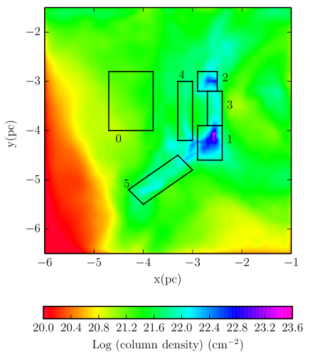
Figure 3: Temperature map and column density map ($N_{\rm H}$) of the high-resolution simulation of Run I of Dale et al. (2012). The boxes represent the regions which contain filaments and cores. Box 0: control field; Boxes 1 & 2: cores; Boxes 3, 4 & 5: filaments. The small protocluster is contained in Box 1.

Figure 4: The left panel presents the column density distributions and the right panel the normalised PDFs of the Serpens Core (in red) and two snapshots of Run I of the simulations of Dale et al. (2012) that differ by 0.4 Myr in time (in blue and green). The snapshot at $t_{SC}$ is shown in Figure 3. The dashed-dotted red lines in the left panel represent the fit of a Gaussian distribution and a power-law. In the right panel the dashed-dotted lines represent the best Gaussian fit of the observations (in red), Run I at $t_{SC}$ (in blue) and Run I at $t_{SC}$+0.4 Myr (in green).

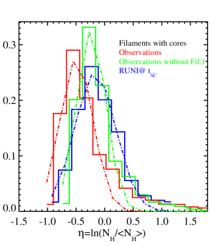
Figure 5: The left panel represents the histograms of the column density distributions while the right panel shows the normalised PDFs of the Filaments with cores. The dashed-dotted lines overplotted to the PDFs represent the best Gaussian fit of the data. Red lines represent the observations, the blue ones represent the simulations, and the green lines represent the observations without Filament number 1. The positions of the observed filaments and cores are highlighted in Figure 2, while the simulated filaments and cores are outlined in Figure 3.

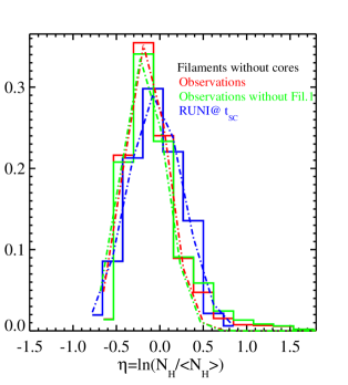
Figure 6: The left panel represents the histograms of the column density distributions while the right panel shows the normalised PDFs of the Filaments without cores. The dashed-dotted lines overplotted to the PDFs represent the best Gaussian fit of the data. The positions of the observed filaments are highlighted in Figure 2, while the simulated filaments are outlined in Figure 3. The different colors of the lines are as in Figure 5.

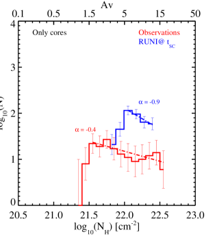
Figure 7: The left panel represents the histograms of the column density distributions while the right panel shows the normalised PDFs of the cores alone. The positions of the observed cores are highlighted in Figure 2, while the simulated cores are outlined in Figure 3. The different colors of the lines are as in Figure 5.

5.2 column density distributions

The column density distribution of the entire field that covers the Serpens Core (as highlighted in Figure 2) is shown in Figure 4 as a red histogram. The observations show a cut at densities lower than 10^20.5 cm^-2, due to the sensitivity limit of the observations. The sensitivity limit is sufficient to well sample the peak in the observed column density distribution, which is more narrow than the peak in the simulations. Overplotted are the column density distributions from two simulation snapshots separated in time by $\approx 0.4$Myr. The distribution evolves relatively little during this period of time.

The slopes of the histograms of column densities have been compared between observations and simulations, as it is shown in Figures 4 to 7. The histograms of column densities of the simulations and the PDFs have been constructed as in the analysis of the observations. The dashed-dotted lines in the left panel of Figure 4 represent the fit of a Gaussian distribution and a power-law. We find that the deviation from a log-normal distribution corresponds to A${}_{\rm v}\sim$1.2-2.0 mag. Both column density distributions of the two snapshots of the simulation separated by 0.4 Myr in time, show a very broad peak resembling a log-normal distribution, but with a pronounced tail at high column densities, rather different from that seen in the observed cloud. In particular, there is a considerable amount of low-density material that does not appear in the observed data (it is below the observational sensitivity limit), and the peak of both simulated distributions occurs at a higher column density. The quantity of high-column density material, between $\approx 10^{22}$ and $10^{23}$ cm^-2 drops between the two simulation snapshots. The quantity of material which appears to be ‘missing’ between the two distributions is $\sim 10$ M_⊙, corresponding to an order of one percent of the total mass of gas in the simulation volume, and to about thirty percent of all gas denser than $10^{22}$ cm^-2. In the 0.4 Myr time interval between the two snapshots some of the high–density gas is consumed by star formation. The figure highlights the fact that, while a simulation snapshot and an observed field may appear subjectively similar, more careful analysis can reveal important differences between them.

The distribution of the observed column densities of all filaments, including the cores, shows a peak at $A_{\rm V}\sim 0.6$ mag, with a maximum value of $A_{\rm V}\sim 18$ mag (see left panel in Figure 5). For $A_{\rm V}\sim$ 1.5 - 14 mag, the distribution decreases as a power-law, following the relation $dlog(N)/dlog(N_{H})\sim\alpha$, where $\alpha\sim-1.3$ (red histogram in the left panel of Figure 5). In the simulations the peak is found at a higher value i.e. $A_{\rm V}\sim 3$ mag. The slope computed between $A_{\rm V}\sim$ 6 - 12 mag is $\alpha\sim-1.6$, i.e. steeper than the observed value.

The core emission has been identified as an enhancement in the column density map, as well a point source emission at least at one Herschel wavelength. In filament number 1 in the Serpens Core, we found two cores (both included in the same box) and in filament number 7 one core. Since all the cores do show a point source counterpart at 70 $\mu$m, this means that we are selecting the more evolved protostellar cores, and not the cores at an earlier evolutionary stage (when they do not have yet 70 $\mu$m emission). In the simulations two cores are identified. The histogram of the filaments without cores, obtained by drawing a box around the cores and excluding them, is computed for both observations and simulations (see left panel of Figure 6). In the observations the maximum column density reaches $A_{\rm V}\sim 9$ mag, and its peak is at $A_{\rm V}\sim 0.7$ mag. While the observations show a peak with a power-law tail with a slope $\alpha\sim-1.5$, the simulations show only a peak at $A_{\rm V}\sim 3$ mag. The slope in the observed filaments becomes steeper excluding the cores.

We also did the analysis of the filaments with and without cores excluding the filament number 1, that is the only supercritical filament in the network of filaments of the Serpens Core. In Figures  5 and  6 the histograms without filament number 1 are drawn in green. In both cases the histogram still shows a power law tail, but with a steeper slope. In the case of the filaments with cores a steeper slope was expected, since by excluding filament 1, we are not considering the two cores that are present in this filament. It is even more interesting to notice that even without the only supercritical filament, the observed filaments still show a power law tail.

A histogram showing the cores alone has been constructed excluding the filaments in both observations and simulations (see left panel of Figure 7). In the case of the simulation the maximum column density reaches a value of $A_{\rm V}\sim 12$ mag, and the slope decreases to an almost flat slope of $\alpha\sim-0.9$. In this case of the cores alone there are not many pixels which sample the cores and the errors are much larger than in the histograms of the column densities of the filaments with and without cores.

5.3 Probability density functions (PDFs) of the filaments.

The PDFs of the same regions described in Section 5.2 have been computed for the observations and simulations and they are shown in the right panels of Figures 4 to  7.

A quantitative comparison between the PDFs of the observations and the simulations has been carried out using the standard non-parametric Kolmogorov-Smirnov statistic test. The computed probability that the observed and simulated distributions are drawn from the same distribution is give in Table 4. We notice that the lowest probability is found in the case of filaments with cores. The value is, however, not sufficiently low to conclude that simulations and observations are from different parent distributions.

We perform a Gaussian fit of each PDF in order to characterise the log-normal function:

$$p_{\eta}d\eta=\frac{1}{\sqrt{2\pi\sigma^{2}_{\eta}}}\exp{\Big{[}-\frac{(\eta-\mu)^{2}}{2\sigma^{2}_{\eta}}\Big{]}}d\eta$$ (3)

where $\sigma_{\eta}$ is the dispersion, and $\mu$ is the mean logarithmic column density. The widths, $\sigma_{\eta}$, resulting from the fitting are reported in Table 4. We notice that the values of $\sigma_{\eta}$ in the observations of the Serpens Core are always lower than the values in the simulations. In the case of the cores alone, the values of $\sigma_{\eta}$ are not meaningful since both, the observed and simulated PDFs do not show any peak.

As for the column density distributions, also the PDFs of the filaments alone in the simulations show only a log-normal distribution while the observed filaments do show a power-law tail (see right and left panel of Figure 6). This is in agreement with the finding that the filaments themselves in the simulations are not fragmenting, but are instead serving as conduits of gas into the main cluster. The simulated cores at higher column densities show instead the power-law tail, while the observed cores have an almost flat distribution (see Figure 7). In the PDFs the log-normal component always dominates compared to the power-law tail and the simulations show always a higher FWHM than the observations, apart from the case of the cores alone. Since the FWHM of the PDFs is a measure of the turbulent dispersion velocity (e.g. Federrath & Klessen 2013), this implies that the turbulent velocities in the observed filaments are always lower than those in the simulation.

A power-law tail in the column density distribution has been interpreted as a transition between a turbulence-dominated gas and a self-gravitating gas (e.g. Klessen 2000; Federrath & Klessen 2013). Studies of the probability distribution functions, computed from the column density maps, have been used to constrain star formation processes. Using the column density maps from Herschel, Schneider et al. (2015) compared the PDFs of low-mass and high-mass star-forming regions, finding a common “threshold” value of A${}_{\rm V}\sim$4-5 mag (corresponding to $N_{\rm H}=$3.8-4.7$\times$10²¹ cm^-2) between turbulence-dominated gas and self-gravitating gas. This “threshold” is higher than the value of A${}_{\rm V}\sim$1.2-2.0 mag that we find in the column density distribution of the Serpens Core (see Figure 4). The column density PDFs presented suggest that the simulated filaments are likely turbulence-dominated, while the observed filaments have the characteristic power-law tails indicating that they are most likely in the self-gravitating regime and that they will probably eventually fragment into cores. A more stringent criterion for gravitational instability which indicates that filaments are already in the process of sub-fragmentation (e.g. André et al. 2010, 2014) is whether their masses per unit length are supercritical. Recent observations by Lee et al. (2014) found that filaments FS1, FS2 and FS3 (which correspond to our filament number 1) do indeed have supercritical values of M/L, while their filaments FC1 and FN1 (our filaments 2 and 4, respectively) have M/L values close to the critical threshold (Table 2), suggesting that they will begin sub-fragmentation very soon.

Table 4: Standard deviation $\sigma_{\eta}$ (defined in Equation 3) of the log-normal distributions overplotted in Figures 4, 5, 6 & 7. The last column shows the probability that the simulated and observational data (the observed filaments refer to numbers 1 to 8) are drawn from the same distribution using the K-S test.

	Serpens Core	Run I @ tSC	PK-S
Entire Field	0.27	0.78	0.54
Filaments with cores	0.28 (0.25)	0.36	0.03
Filaments without cores	0.24 (0.25)	0.32	0.19
Control field	0.13	0.38	0.36

6 Summary and Conclusions

In this paper we analyze continuum Herschel observations of the Serpens Core and compare them to a numerical simulation from the suite of calculations performed by Dale et al. (2012). Since the Serpens Core does not harbor any high-mass star, we choose an early state of a particular simulation of Dale et al. (2012) before any O–stars have formed and therefore without any feedback. It is possible that this region will form high–mass stars in the future, since it has a substantial reservoir of gas available and its maximum column density is only a factor of a few lower than the canonical 1 g cm^-2 threshold for massive star formation proposed by Krumholz & McKee (2008). In the chosen simulation, the action of the filaments is mainly to deliver more gas into the cluster which forms at the hub where they join, without fragmenting. We selected a sub-region of Run I with the most similar total mass, spatial scale and morphology to the Serpens Core. We then compared the properties, such as temperature and surface density in regions identified by the presence of a filamentary structure or a core. Note that the simulation was not designed to produce an object resembling Serpens (or any other star–forming region). The resemblance is serendipitous and owes to the aim of Dale et al. (2012) to cover a realistic parameter–space with general simulations. The picture which emerges is rather complex. With the additional time dimension available in the simulations, we saw that, while the simulations and observations may appear similar in morphology at a given time, they may differ in other respects, such as in the form of the column density distribution. Advancing the simulation in time resulted in the morphological disparity increasing, but the two datasets becoming more similar from the point of view of their column density distributions. This indicates that quantitatively comparing simulations and observations is more difficult than it may firstly appear. We defer a more detailed analysis to a later paper in which we construct synthetic observations of the simulations in order to make such a comparison more robust.

The main results and conclusions of our study can be summarized as follows:

1. Herschel continuum observations between 70 and 500 $\mu$m reveal a radial network of filaments converging into the central cluster of the Serpens Core: this low-mass star forming region has been used to test the state-of-the-art of simulations of GMCs.

2. In the filaments the dust temperatures are found to lie in the range between 12 K and 19 K in the observations and few Kelvin lower than the gas temperatures in the simulations: this might reflect a difference in temperature between gas and dust in the region.

3. The peak in the observed column density distribution of the entire field of the Serpens Core is more narrow than the peak in the simulations. Both distribution show a power-law tail at higher column densities but with different slopes. This can be explained by a different evolutionary stage of the simulation in comparison to the real observations.

4. The peaks in the column density distributions of the filaments are about $10^{0.5}$ cm^-2 higher in the simulation than those in the observations.

5. From the measured widths, $\sigma_{\eta}$, of the PDFs, we found that the turbulent velocities in the observed filaments are likely lower than those in the simulations.

6. The column density distribution and PDFs of simulated filaments shows only a log-normal distribution, while the observed filaments show a power-law tail. The power-law tail becomes evident in the simulation in the column density distribution of the cores, while in the observations this shows a flat distribution. This means that while the simulated filaments are likely turbulence-dominated regions, the observed filaments are probably turbulence-dominated self-gravitating structures which will fragment into cores.

   In the simulation, the main function of the filaments is to feed gas into the central cluster which is where most of the star formation takes place. Most of the gas in the filaments falls into the cluster before fragmenting. It is therefore possible that, despite the physical and morphological similarities between the chosen simulation timesteps and the Serpens Core, the filaments in the real and simulated clouds are behaving in very different ways. Whether this is due to neglected physics in the simulations (e.g. magnetic fields), to unknown differences between the early phases of the Serpens Core and the initial conditions of the calculations, or just to the extreme difficulty of comparing two very complex dynamical systems is not clear. The simulated and observed filaments are subjectively similar–looking, but behave differently, the former being turbulence-dominated and the latter being self-gravitating.

Appendix A The Control field

We consider in both observations and simulations a control region where neither filamentary structures nor cores are present (box 0 in Figures 2 and 3). Figure 8 shows the histograms of the column density distributions on the left, and the PDFs on the right. Since only few bins are covered in the column density distribution, these plots are shown in the appendix. However, the small error-bars in each bin highlight that the column density distributions show only a peak without any additional structure. This peak at $A_{\rm V}\sim 0.5$ mag is very narrow in the observations, while in the simulations the peak is much broader.

Figure 8: The left panel represents the histograms of the column density distributions of the control field, while the right panel the PDFs. The dashed lines overplotted to the PDFs represent the best Gaussian fit of the data. Red lines represent the observations, while the blue ones represent the simulations.

Appendix B Filamentary structures in the Serpens Core.

Figure 9 shows the enlargements on Filament number 1: starting from the left side, the first five panels show the Herschel PACS and SPIRE mosaics, while the last two panels show the column density and the temperature map. An additional box identifies the position of a core structure among the filament.

Figure 9: Filament number 1. Starting from the left side, the panels show Herschel/PACS 70 $\mu$m, 160  $\mu$m, and SPIRE 250 $\mu$m, 350 $\mu$m, and 500 $\mu$m, respectively. The unit of all the images is Jy/arcsec². The last two panels show the column density map ($N_{\rm H}$) in [$\times$10${}^{+20}cm^{-2}$] and the temperature map in ${\rm K}$. The box identifies the extension of the filament and its size is listed in Table 2. The smaller box identifies the position of the cores among the filament.

In the online material, Figures 8- 16 show the enlargements on each filament as in Figure 9.

Figure 8: Filament number 1. Starting from the left side, the panels show Herschel/PACS 70 $\mu$m, 160  $\mu$m, and SPIRE 250 $\mu$m, 350 $\mu$m, and 500 $\mu$m, respectively. The unit of all the images is Jy/arcsec². The last two panels show the column density map ($N_{\rm H}$) in [$\times$10${}^{+20}cm^{-2}$] and the temperature map in ${\rm K}$. The box identifies the extension of the filament and its size is listed in Table 2. The smaller box identifies the position of the cores among the filament.

Figure 9: Filament number 2. The panels and the units are as in Figure 8.

Figure 10: Filament number 3. The panels and the units are as in Figure 8.

Figure 11: Filament number 4. The panels and the units are as in Figure 8.

Figure 12: Filament number 5. The panels and the units are as in Figure 8.

Figure 13: Filament number 6. The panels and the units are as in Figure 8.

Figure 14: Filament number 7. The panels and the units are as in Figure 8. The smaller box identifies the position of the core among the filament.

Figure 15: Filament number 8. The panels and the units are as in Figure 8.

Figure 16: Filament number 9. The panels and the units are as in Figure 8.