Caliber based spectral gap optimization of order parameters (SGOOP) for sampling complex molecular systems

Abstract

In modern day simulations of many-body systems much of the computational complexity is shifted to the identification of slowly changing molecular order parameters called collective variables (CV) or reaction coordinates. A vast array of enhanced sampling methods are based on the identification and biasing of these low-dimensional order parameters, whose fluctuations are important in driving rare events of interest. Here describe a new algorithm for finding optimal low-dimensional collective variables for use in enhanced sampling biasing methods like umbrella sampling, metadynamics and related methods, when limited prior static and dynamic information is known about the system, and a much larger set of candidate CVs is specified. The algorithm involves estimating the best combination of these candidate CVs, as quantified by a maximum path entropy estimate of the spectral gap for dynamics viewed as a function of that CV. Through multiple practical examples, we show how this post-processing procedure can lead to optimization of CV and several orders of magnitude improvement in the convergence of the free energy calculated through metadynamics, essentially giving the ability to extract useful information even from unsuccessful metadynamics runs.

I Introduction

With the advent of increasingly accurate force-fields and powerful computers, Molecular Dynamics (MD) simulations have become an ubiquitous tool for studying the static and dynamic properties of systems across disciplines. However, most realistic systems of interest are characterized by deep, multiple free energy basins separated by high barriers. The timescales associated with escaping such barriers can be formidably high compared to what is accessible with straightforward MD even with the most powerful computing resources. Thus in order to accurately characterize such landscapes with atomistic simulations, a large number of enhanced sampling schemes have become popular, starting with the pioneering works of Torrie, Valleau, Bennett and others Bolhuis et al. (2002); Torrie and Valleau (1977); Carter et al. (1989); Hansmann and Okamoto (1993); voter_prl ; Laio and Parrinello (2002); Barducci, Bussi, and Parrinello (2008); Darve, Rodríguez-Gómez, and Pohorille (2008); Abrams and Vanden-Eijnden (2010); Zheng, Chen, and Yang (2008); Tiwary and van de Walle (2013). Many of these schemes involve probing the probability distribution along selected low-dimensional collective variables (CVs), either through a static pre-existing bias or through a bias constructed on-the-fly, that enhances the sampling of hard to access but important regions in the configuration space.

The quality, reliability, and usefulness of the sampled distribution is in the end deeply dependent on the quality of the chosen CV. Specifically, one key assumption inherent in several enhanced sampling methods is that of time-scale separation Berezhkovskii and Szabo (2011): for efficient and accurate sampling, the chosen CV should encode all the relevant slow dynamics in the system, and any dynamics not captured by the CV should be relatively fast. For most practical applications, there are a large number of possible CVs that could be chosen, and it is not at all obvious how to construct the best low-dimensional CV or CVs for biasing from these various possible options. Success in enhanced sampling simulations has traditionally relied on an apt use of physical intuition to construct such low dimensional CVs. Identification of good low dimensional CVs is in fact useful not just for enhanced sampling simulations such as umbrella sampling and metadynamics but also for distributed computing techniques like Markov State Models (MSM) Pérez-Hernández et al. (2013), allowing one to significantly improve the quality and reliability of the constructed kinetic models. Last but not the least, having an optimal low dimensional CV can also help in the building of Brownian dynamics type models Ermak and McCammon (1978); Morrone, Li, and Berne (2011). Indeed, given the importance of this problem, there exists a range of methods that have been proposed to solve it Best and Hummer (2005); Coifman et al. (2005); Peters and Trout (2006); Ma and Dinner (2005); Rohrdanz et al. (2011); Ceriotti, Tribello, and Parrinello (2011); Chen, Yu, and Tuckerman (2015); Salvalaglio, Tiwary, and Parrinello (2014).

In this communication, we report a new and computationally efficient algorithm for designing good low-dimensional slow CVs. We suggest that the best CV is one with the maximum separation of timescales between visible slow and hidden fast processes Coifman et al. (2008); Berezhkovskii and Szabo (2011), or the maximum spectral gap. The method is named spectral gap optimization of order parameters (SGOOP). Note that in this work henceforth we refer to the best CV in the singular, without loss of any generality in the treatment. The notion of such a timescale separation is at the core of not just enhanced sampling methods but also coarse-grained, Multiscale and projection operator methods Berne and Pecora (2000); Car and Parrinello (1985); Kevrekidis (2003).

Our algorithm involves learning the best linear or non-linear combination of given candidate CVs, as quantified by a maximum path entropy Pressé et al. (2013) estimate of the spectral gap for the dynamics of that CV. The input to the algorithm is any available information about the static and dynamic properties of the system, accumulated through (i) a biased simulation performed along a sub-optimal trial CV, possibly (but not necessarily) complemented by (ii) short bursts of unbiased MD runs, or (iii) by knowledge of experimental observables. Any type of biased simulation could be used in (i), as long as it allows projecting the stationary probability density estimate on generic CVs without having to repeat the simulation. Metadynamics Tiwary and Parrinello (2015) provides this functionality in a straightforward manner and hence it is our method of choice here. Given this information we use the principle of Maximum Caliber Pressé et al. (2013); Dixit et al. (2015a) to set up an unbiased master equation for the dynamics of various trial CVs. Through a simple post-processing optimization procedure we then find the CV with the maximal spectral gap of the associated transfer matrix. For instance, this optimization can be performed through a simulated annealing approach that maximizes the spectral gap by performing a robust global search in the space of trial CVs.

Figure 1: In (a), we provide the 2-d De Leon-Berne potential De Leon and Berne (1981) with several candidate path CVs imposed on it. Black circles denote the corresponding milestones Branduardi, Gervasio, and Parrinello (2007). See SI for further details of the CVs. In (b), the corresponding eigenvalues $\lambda_{1}$ and $\lambda_{2}$ (i.e. excluding the stationary eigenvalue $\lambda_{0}$) are shown for each of these paths. As per the spectral gap given here by $\lambda_{1}-\lambda_{2}$, we identify two possible good paths marked with black circles in (b) and correspondingly with thicker black lines in (a). Energy is in absolute units and $k_{B}T=0.1$.

Through three practical examples, we show how our post-processing procedure can lead to better choices of CVs, and to several orders of magnitude improvement in the convergence of the free energy calculated through the popular enhanced sampling technique metadynamics. Furthermore, the algorithm is generally applicable irrespective of the number of stable basins. Our algorithm essentially provides the much needed ability to extract useful information about relevant CVs even from unsuccessful metadynamics runs. In addition to use in free energy sampling methods, the optimized CV can then also be used in other methods that provide kinetic rate constantsTiwary and Parrinello (2013); Tiwary et al. (2015a). We expect this algorithm to be of widespread use in designing CVs for biasing during enhanced sampling simulations, making the process significantly more automatic and far less reliant on human intuition.

II Theory

Let us consider a molecular system with $N$ atoms at temperature $T$. We assume there exists a large number $d$ of available order parameters with $1\ll d\ll N$, collectively referred to as $\{\Theta\}$, such that the dynamics in this $d-$dimensional space is Markovian. These could be inter-molecular distances Best and Hummer (2005), torsional angles, solvation states, nucleus size/shape ten Wolde, Ruiz-Montero, and Frenkel (1999), bond order parameters Steinhardt, Nelson, and Ronchetti (1983) etc. The identification of such order parameters poses another complicated problem, but as routinely done in other methods aimed at optimizing CVs Best and Hummer (2005); Pérez-Hernández et al. (2013); Chen, Yu, and Tuckerman (2015), we assume such order parameters are a priori known.

There are several available biasing techniques that can sample the probability distribution of the space $\{\Theta\}$, and even calculate the rate constants for escape from stable states in this space Tiwary and Parrinello (2013). All of these techniques are feasible only for a very small number of CVs whose number is much smaller than $d$ - typically one to three. These are the order parameters whose fluctuations are deemed to be most important for the system or process being studied, and by building a fixed or time-dependent bias of these CVs, one should be able to determine the true unbiased probability distribution of the full space $\{\Theta\}$. But how does one decide what is an optimal low-dimensional subset or combination of the available order parameters? This dimensionality reduction is of central importance to methods such as umbrella sampling, metadynamics and others, the answer to which decides the speed of convergence of the biased simulation, or if it it will even ever converge within practically useful simulation times.

Figure 2: (a) The 5-residue peptide studied in this work. The six dihedral angles are marked. (b) The output of the simulated annealing algorithm run separately for different $\theta_{0}$ values (blue circles). The starting value with the trial choice of CV is marked with a magenta colored star. (c) The trial (magenta) and optimized (blue) mixing coefficients $\{c\}$ for the 6 dihedrals. (d) The spectrum of eigenvalues for dynamics projected on the trial (magenta) and optimized (blue) CVs. A distinct improvement can be seen in the spectral gap.

The key idea in the current work is to perform enhanced sampling (e.g. metadynamics) with a choice of trial CVs, complemented by information gathered from short bursts of unbiased MD simulations and experimental observables when available, to iteratively improve the CVs. The maximum Caliber framework Jaynes (1980); Pressé et al. (2013); Dixit et al. (2015a, b), which is a dynamical generalization of the hugely popular maximum entropy framework Jaynes (1957), provides a method for accomplishing this.

We start by choosing a trial CV given by $f\{\Theta\}$, where $f$ maps the space $\{\Theta\}$ onto a lower dimensional space. The space along this trial CV $f\{\Theta\}$ is then discretized in grids labeled $n$. This CV could be multi-dimensional, with $n$ then indexing the multidimensional grids. Let $p_{n}(t)$ denote the instantaneous probability of the system being found in grid $n$. For the sake of clarity, we assume that $f$ is a linear combination of $\{\Theta\}$, i.e. $f=c_{1}\Theta_{1}+c_{2}\Theta_{2}+...+c_{d}\Theta_{d}$. The treatment developed here applies to non-linear combinations as well which we show in the examples. Then, for a fixed $\Delta t$, we write a master equation:

$${\Delta p_{n}(t)\over\Delta t}=\Sigma_{m}\omega_{mn}p_{m}(t)-\Sigma_{m}\omega_{nm}p_{n}(t)\equiv\Sigma_{m}\Omega_{nm}p_{m}(t)$$ (1)

where $\omega_{nm}$ is the rate of transition from grid $n$ to $m$ per unit time. The matrix $\Omega_{nm}$ is the entirety of all these rates. If the dynamics of $f\{\Theta\}$ is Markovian, then the matrix $\bf{k}$ of transition probabilities is given for small $\Delta t$ by

$${\bf k}=\exp({\bf{\Omega}}{{\Delta t}})\approx{\bf I}+{\bf\Omega}{\Delta t}$$ (2)

should not depend on the value of $\Delta t$ used in Eq. 1. This provides a self-consistency check of whether or not the CV so generated is Markovian. In the maximum Caliber approach one uses all available stationary state and dynamical information to construct probabilities of micropaths. Instead of defining the entropy as a function of microstate probabilities as in information theory and statistical thermodynamics Jaynes (1957), one now defines an entropy $S$ as a functional of the probabilities of micropaths, which is essentially a path integral. For the Markovian process of Eq.1 Filyukov and Karpov (1967):

$$S=-\Sigma_{ab}p_{a}k_{ab}\text{ log }k_{ab}$$ (3)

Path ensemble averages of time-dependent quantities $A_{ab}$ can now be calculated as follows Pressé et al. (2013); Dixit et al. (2015a), where the subscripts $a$,$b$ denote grid indices:

$$\langle A\rangle=\Sigma_{ab}p_{a}k_{ab}A_{ab}$$ (4)

The path entropy of Eq. 3 incremented by quantities accounting for constraints placed by our knowledge of observables $\{\langle A^{n}_{ab}\rangle\}$, and some other constraints such as detailed balance, is collectively called Caliber Pressé et al. (2013); Dixit et al. (2015a). Maximizing the Caliber is then equivalent to being least non-committal about missing dynamic and static information, with the end result being that one obtains a relation between the grid-to-grid rates and the stationary probabilities as follows:

$$\omega_{ab}={1\over\Delta t}{\sqrt{p_{b}\over p_{a}}}e^{-\Sigma_{i}\rho_{i}A_{ab}^{i}}$$ (5)

Here $i$ runs over the number of available dynamical pieces of information, and $\rho_{i}$ is the Lagrange multiplier for the associated constraint. As a special case, consider when the only observable at hand is the mean number of transitions in observation interval $\Delta t$ over the $entire$ grid Dixit et al. (2015a) along a trial CV. In this case, the above equation takes a particularly simple and useful form:

$$\omega_{ab}={1\over\Delta t}{\sqrt{p_{b}\over p_{a}}}e^{-\rho}$$ (6)

Our method then involves calculating for various trial CVs the spectral gap of the transition probability matrix k, which for $a\neq b$ is $k_{ab}=\omega_{ab}\Delta t$ and satisfies normalization $\Sigma_{b}k_{ab}=1$. Let $\{\lambda\}$ denote the set of eigenvalues of k, with $\lambda_{0}\equiv 1>\lambda_{1}\geq\lambda_{2}...$. The spectral gap is then defined as $\lambda_{s}-\lambda_{s+1}$, where $s$ is the number of barriers apparent from the free energy estimate projected on the CV at hand, that are higher than a user-defined threshold (typically $\gtrsim k_{B}T$). Estimating the Lagrange multiplier is computationally expensive, so a first estimate for maximizing the spectral gap is performed using Eq. 6 where the Lagrange multiplier $\rho$ need not be computed. Also note that in the limit of small $\Delta t$, the matrix k will be diagonally dominated Rosta and Hummer (2014), and to estimate the spectral gap one needs only an accurate estimate of relative local free energies. More static or dynamical information Bicout and Szabo (1998); Hummer (2005); Marinelli et al. (2009); Berne, Pechukas, and Harp (1968); Granata et al. (2013); Bonomi et al. (2015) simply introduces additional Lagrange multipliers and can be treated through Eq. 5. This can be done if the intention is to calculate an accurate kinetic model with correct estimates of the dominant eigenvalues and not just the spectral gap.

We are now in a position to describe the actual algorithm. It comprises the following two steps in a sequential manner, and can be improved by iterating.

1. Perform metadynamics along a trial CV $f=c_{1}\Theta_{1}+c_{2}\Theta_{2}+...+c_{d}\Theta_{d}$ to get a crude estimate of the stationary density.

2. As post-processing, perform optimization in the space of mixing coefficients $\{c_{1},c_{2}...c_{d}\}$ to identify the CV with the maximal spectral gap. The reweighting functionality Tiwary and Parrinello (2015) of metadynamics allows projection of free energy estimates on different CVs with minimal computational effort, and is used to calculate the k matrix through Eq. 6. We elaborate on the optimization procedure details in the next section (Illustrative Examples).

The optimization procedure gives the best CV as the one with highest spectral gap, given the information at hand. As in any maximum entropy framework Jaynes (1957), the better the quality of this information, the more accurate will be the spectral gap. But even with very poor quality information, as we show in the examples, the algorithm still leads to significant improvements in the CV. Furthermore, whether or not the CV is Markovian can also be checked by repeating step 2 for different time intervals $\Delta t$ of observation and determining if the spectral gap is independent of the value of $\Delta t$.

Figure 3: (a) and (b) show trajectories obtained from metadynamics biasing the trial CV and the optimized CV respectively. First 20 ns of the trajectory shown in (a) was used to generate the optimized CV for (b). A very pronounced improvement in the enhancement of sampling can be seen with the optimized CV.

III Illustrative Examples

III.1 Model 2-d landscapes: The De Leon-Berne potential

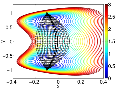
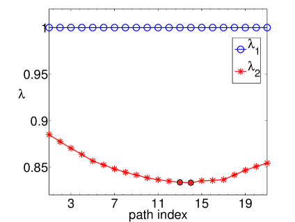
The first illustrative example for SGOOP is a model 2-state potential introduced by De Leon and Berne De Leon and Berne (1981). To sample this landscape at temperature $k_{B}T=0.1$, we perform metadynamics with path CVs, a class of widely used CVs that can capture non-local and non-linear fluctuations (see Branduardi, Gervasio, and Parrinello (2007) for details). Path CVs require specification of a series of milestones between two points in configuration space, where the milestones can be described in terms of generic order parameters. Fluctuations in the system can then be enhanced in the direction along and perpendicular to these milestones, leading to efficient exploration of the space. In Fig. 1 (a) we show the 2-d potential along with several possible path CVs imposed on it. We first perform a short trial metadynamics run biasing the y-coordinate. By post-processing this, we generate the spectral gaps for various paths using Eq. 6 (Fig. 1 (b)). By comparing Fig. 1(a) against Fig. 1(b), it is clear how the path with maximum spectral gap is the minimum energy pathway passing through the saddle point. In this case while this result could have simply been obtained through Nudged Elastic Band type calculations Henkelman, Uberuaga, and Jónsson (2000) - the point is to use this example to develop intuition for the method. Also note that moving around the best path to others that are a bit distant from it, does not lead to much change in the spectral gap. This is consistent with the observation that in several enhanced sampling methods such as metadynamics or umbrella sampling Torrie and Valleau (1977); Laio and Parrinello (2002); Barducci, Bussi, and Parrinello (2008), the CV need not be precisely the true reaction coordinate, as long as it has a sufficient overlap with it Branduardi, Gervasio, and Parrinello (2007); Tiwary et al. (2015b).

In the Supplemental Information (SI), we provide a similar analysis on another 2-d model potential but with 3 states. The conclusions are similar.

III.2 5-residue peptide

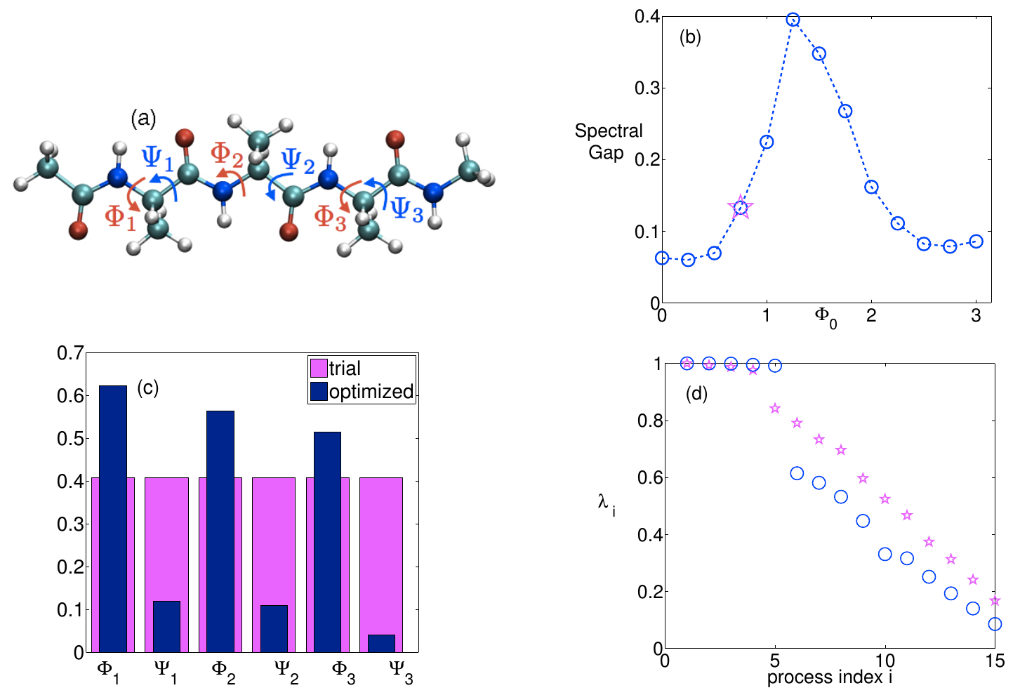
Now we move to a more complex system, which has also been considered as a test case for new enhanced sampling methods Valsson and Parrinello (2014) in order to establish their usefulness. This is the 5-residue peptide $Ace-Ala_{3}-Nme$ in vacuum (see Fig. 2 (a)), where there are six possibly relevant dihedral torsion angles. Here we ask the question: what is the best possible 1-d linear combination of these six dihedrals that we could bias but still maximally enhance exploration of the 6-d space comprising all the dihedrals?

Figure 4: Errors in the 1-d free energies in kJ calculated with respect to reference free energies Valsson and Parrinello (2014, 2015) using the error metric from Branduardi, Bussi, and Parrinello (2012). Thin and thick lines denote values using the trial and optimized CVs respectively.

In this problem, for periodicity related numerical reasons, we bias a reference cosine defined by cos($\theta-\theta_{0}$), where $\theta$ is one of the six dihedral angles, and $\theta_{0}$ is some reference value whose optimal choice we do not know a priori. Through our algorithm we then seek to identify:

1. The best choice of mixing coefficients $\{c\}$ to use in trial CV $f=c_{1}\Phi_{1}^{\prime}+c_{2}\Psi_{1}^{\prime}+c_{3}\Phi_{2}^{\prime}+c_{4}\Psi_{2}^{\prime}+c_{5}\Phi_{3}^{\prime}+c_{6}\Psi_{3}^{\prime}$, where we keep the euclidean norm of $\{c\}$=1, and for any angle $\theta$ the prime denotes the transformation $\theta\mapsto 0.5+cos(\theta-\theta_{0})$.

2. The best choice of $\theta_{0}$, kept same for all 6 dihedrals.

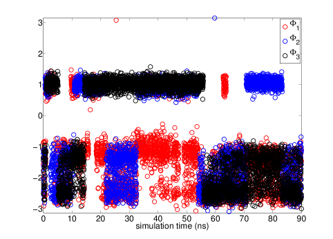
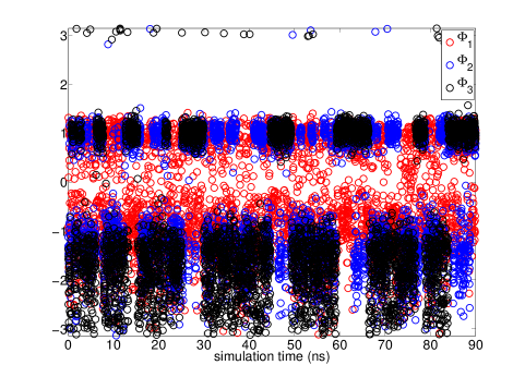
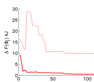
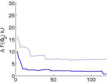
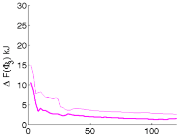
We start with the trial CV where all members of $\{c\}$ are the same subject to euclidean norm of $\{c\}$=1, and an arbitrary choice of $\theta_{0}=0.75$ radians is taken. A short metadynamics run is performed biasing this trial CV. See supplemental information (SI) for details of the metadynamics and MD parameters Tribello et al. (2014), and Fig. 3 (a) for the metadynamics trajectory used for spectral gap optimization. Based on the free energy estimate generated from this run, a simulated annealing procedure is performed in the space $\{c\}$ for various $\theta_{0}$ values. Starting from the spectral gap estimated using Eq. 6 for the trial CV, this involves executing Metropolis moves in the $\{c\}$ space with an attempt to find the global maxima of the spectral gap. In Fig. 2 (b-d) respectively, we show how the spectral gap is increased by the simulated annealing procedure, and the corresponding best estimate of $\{c,\theta_{0}\}$. The algorithm suggests the minimal role of the angles $\Psi_{1},\Psi_{2},\Psi_{3}$ as can be seen through their relatively low weights Valsson and Parrinello (2014) (Fig. 2 (c)). The spectrum of eigenvalues for dynamics projected on the trial (magenta) and optimized (blue) CVs, along with respective spectral gaps is provided in Fig. 2(d). Fig. 3 (a-b) show the metadynamics trajectories for the three dihedral angles $\Phi_{1},\Phi_{2},\Phi_{3}$ with the trial and the optimized CVs respectively. A very pronounced improvement in the quality of sampling can be seen. Fig. 4 (a-c) shows the rate of convergence of the error of the estimated free energy Tiwary and Parrinello (2015) with respect to reference values from other approaches Valsson and Parrinello (2014), through metadynamics runs performed with each of the trial and optimized CVs respectively. The error metric is the same as in Branduardi, Bussi, and Parrinello (2012); Valsson and Parrinello (2014), and is calculated for all points within 25 kJ of the global minimum in the respective 1-d free energy. The behavior is robust with respect to the choice of this threshold value. As can be seen, the optimized CV, even though it was obtained on the basis of a very poorly converged and short (20 ns) metadynamics run, leads to several orders of magnitudes improvement in the rate at which the free energies converge. Interestingly, iterating the algorithm with the improved 1-d CV did not lead to much improvement in the sampling, reflecting that the optimized coefficients $\{c\}$ are close to the best that can be achieved with a 1-d CV for this problem.

IV Conclusions

To conclude, we have introduced a new approach named SGOOP (spectral gap optimization of order parameters) for improving the choice of low-dimensional CVs for biasing in enhanced sampling in complex systems. This is accomplished through the use of maximum Caliber based spectral gap estimates. The algorithm is iterative in spirit, and attempts to learn how to improve CVs based on available stationary and dynamic data. We also provide several proof-of-concept practical examples to establish the potential usefulness of the method. For model 2-d potentials the algorithm was shown to yield the minimum energy pathway. For a small peptide, we found very significant improvement in determining the best 1-d collective variable from six possible functions with no ad hoc or intuition based tuning. Future work will use this algorithm to treat a range of problems, especially involving protein-ligand unbinding. For instance, the displacement of water molecules and protein flexibility are often slowly varying order parameters in unbinding Tiwary et al. (2015b); Ladbury (1996); Berne, Weeks, and Zhou (2009); Tiwary et al. (2015a), but do we really need to bias one or both of these for the purpose of sampling? Another issue to be considered in future work is can we use these optimized CVs to obtain reliable dynamical information from metadynamics Tiwary and Parrinello (2013); Salvalaglio, Tiwary, and Parrinello (2014), including the very important off-rate for ligand unbinding Copeland, Pompliano, and Meek (2006); Tiwary et al. (2015b).

One central limitation of this algorithm is having to specify possibly a large number of order parameters that may be important. But for many physical problems one does have a sense of which order parameters could be at work, and this is where we expect this algorithm to be of tremendous use. Another obvious limitation is with systems devoid of a time scale separation Zwanzig (1990) - for example, in glassy systems where there is an effectively continuous spectrum of eigenvalues with no discernible time scale separation. However, the dynamics of many complex and real-world molecular systems does thankfully show a time scale separation between few relevant slow modes and remaining fast ones Machta et al. (2013), and we expect our algorithm to be of help in unraveling the thermodynamics and dynamics in such systems.