Synthetic spin-orbit coupling in an optical lattice clock

Abstract

We propose the use of optical lattice clocks operated with fermionic alkaline-earth-atoms to study spin-orbit coupling (SOC) in interacting many-body systems. The SOC emerges naturally during the clock interrogation when atoms are allowed to tunnel and accumulate a phase set by the ratio of the “magic” lattice wavelength to the clock transition wavelength. We demonstrate how standard protocols such as Rabi and Ramsey spectroscopy, that take advantage of the sub-Hertz resolution of state-of-the-art clock lasers, can perform momentum-resolved band tomography and determine SOC-induced $s$-wave collisions in nuclear spin polarized fermions. By adding a second counter-propagating clock beam a sliding superlattice can be implemented and used for controlled atom transport and as a probe of $p$ and $s$-wave interactions. The proposed spectroscopic probes provide clean and well-resolved signatures at current clock operating temperatures.

The recent implementation of synthetic gauge fields and spin-orbit coupling (SOC) in neutral atomic gases  Galitski2013 ; NigelCooperReview ; Dalibard ; Spielmanreview ; Zhang2015 ; Stuhl_spielman ; Mancini_Fallani is a groundbreaking step towards the ultimate goal of using these fully-controllable systems to synthesize and probe novel topological states of matter. So far optical Raman transitions have been used to couple different internal (e.g. hyperfine) states while transferring net momentum to the atoms. However, in alkali atoms Raman-induced spin-flips inevitably suffer from heating mechanisms associated with spontaneous emission. While this issue has not yet been an impediment for the investigation of non-interacting processes or mean field effects Spielmanreview ; Zhang2015 , it could limit the ability to observe interacting many-body phenomena that manifest at longer timescales. Finding alternative, more resilient methods for generating synthetic SOC, and probing its interplay with interactions, is thus highly desirable.

To reduce heating, the use of atoms with richer internal structure such as alkaline-earth-atoms (AEAs) Dalibard ; Mancini_Fallani or lanthanide atoms such as Dy and Er Hui2013 have been suggested. Here, we propose an implementation of SOC using cold AEAs in an optical lattice clock (OLC) OLCs and discuss how SOC physics can be probed in interacting many-body systems. Our proposal relies on the fact that SOC naturally arises in OLCs because the clock laser imprints a phase that varies significantly from one lattice site to the next as it drives an ultra-narrow optical transition. Our proposal offers several advantages over prior schemes. It uses a direct transition to a long-lived electronic clock state with natural lifetime $\gtrsim 10^{2}$ s Boyd2006 , and thus heating from spontaneous emission is negligible. Second, our proposal takes advantage of the sub-Hz resolution of clock lasers Bloom ; Nicholson ; Hinkley ; Katori . Finally, we can probe the interplay of interactions and SOC by operating in the regime where the interaction energy per particle, $U$, is weak compared to the characteristic trapping energies  Martin_2013 ; lemke2011 ; SUN2 ; Rey_Annals ; losses1 ; losses2 but comparable to SOC scales determined by $J$, the tunneling, and $\Omega$, the clock Rabi frequency.

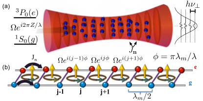
Figure 1: (Color online) (a) A clock laser along the $Z$ direction of wavelength $\lambda$ and Rabi frequency $\Omega$ interrogates the ${}^{1}S_{0}(g)$-${}^{3}P_{0}(e)$ transition in fermionic alkaline-earth atoms trapped in an optical lattice with magic wavelength $\lambda_{m}$. The transverse confinement is provided by Gaussian curvature of the lattice beams with harmonic frequency $h\nu_{\perp}$. Many transverse modes $\mathbf{n}$ are populated at current operating temperatures. (b) The phase difference $\phi$ between adjacent sites $j$ and $(j+1)$ induces SOC when atoms can tunnel with mode-dependent tunnel-coupling $J_{\mathbf{n}}$, realizing a synthetic two-leg ladder with flux $\phi$ per plaquette.

We propose three protocols for probing SOC in an OLC and demonstrate that all provide clear signatures under current operating conditions. In the first protocol, we demonstrate that momentum-resolved tomography of chiral band structures can be performed using Rabi spectroscopy in the parameter regime $J\sim\Omega\gg U$. In the second protocol we show that the modification of collisional properties by SOC Williams ; Zhang is manifest in standard Ramsey spectroscopy, focusing on the parameter regime $J\gtrsim U$. In the final protocol, controlled and spatially resolved atomic transport Thouless ; TroyerPump ; KwekPump ; MuellerPump ; CooperRey ; Blochpump ; Takahasipump ; Spielmanpump is induced by an additional counter-propagating clock beam that exhibits a controllable phase difference with respect to the original probe beam, and interaction effects beyond mean field modify the dynamics in the parameter regime $\Omega\gg J\sim U$. Although inelastic collisions in the excited state impose limitations in the probing time losses1 ; losses2 ; Scazza ; Cappelinni , we also show that they can be used as a resource for state preparation and readout.

SOC implementation Current OLCs interrogate the ${}^{1}S_{0}(g)$-${}^{3}P_{0}(e)$ transition of ensembles of thousands of nuclear spin polarized fermionic AEAs trapped in a deep 1D optical lattice that splits the gas in arrays of 2D pancakes OLCs (see Fig.1). The lattice potential uses the magic-wavelength, $\lambda_{m}$ to generate identical trapping conditions for the two states. At current operating temperatures, $T\sim\mu$K Martin_2013 the population of higher axial bands is negligible ($\lesssim 5\%$). On the other hand, along the transverse directions, where the confinement is provided wholly by the Gaussian curvature of the optical lattice beams, modes are thermally populated with an average number of mode quanta $\langle n\rangle\sim 50$. To generate SOC coherent tunneling between lattice sites is required. Our proposal is to superimpose a running-wave beam on the lattice potential:

$$\textstyle V_{\mathrm{ext}}\left(\mathbf{R}\right) =\textstyle-\exp\left(-\frac{2R^{2}}{w_{0}^{2}}\right)\left[V_{\mathrm{const}}+V\cos^{2}\left(\frac{2\pi Z}{\lambda_{m}}\right)\right]\,;$$ (1)

this increases the transverse confinement without significantly affecting the axial motion Wall_Hazzard_15 . Here, $w_{0}$ is the beam waist, $R$ the transverse radial coordinate, $Z$ the axial coordinate, $V$ the axial lattice corrugation, and $V_{\mathrm{const}}$ the running-wave induced potential. By increasing $V_{\mathrm{const}}$ as $V$ is lowered, the transverse confinement frequency $\nu_{\perp}\sim\sqrt{\frac{1}{m\pi^{2}w_{0}^{2}}(V_{\mathrm{const}}+V)}$ is kept constant while the tunneling rate along the axial direction increases. Here $m$ is the atom mass.

Since $V_{\mathrm{ext}}\left(\mathbf{R}\right)$ is discretely translationally invariant along the axial direction, atoms trapped in the lowest axial lattice band are governed by the Hamiltonian $\hat{H}^{0}=\sum_{\mathbf{n}}\hat{H}^{0}_{\mathbf{n}}$ Supp

$$\hat{H}^{0}_{\mathbf{n}}=\sum_{q,\alpha}E_{\alpha,\mathbf{n},q}\hat{n}_{\alpha,\mathbf{n},q}-\sum_{q}\left[\frac{\Omega_{\mathbf{n}}}{2}\hat{a}^{\dagger}_{+,\mathbf{n},q+\phi}\hat{a}_{-,\mathbf{n},q}+\mathrm{H.c.}\right]\,.$$ (2)

Here and throughout $q=\tilde{q}a$ is the dimensionless product of axial quasimomentum $\tilde{q}$ and lattice spacing $a=\lambda_{m}/2$, $\hat{a}_{\alpha,\mathbf{n},q}$ annihilates a fermion in the two-dimensional transverse mode $\mathbf{n}$, quasimomentum $q$, state $\alpha=\pm$(for $e$ and $g$), and $\hat{n}_{\alpha,\mathbf{n},q}=\hat{a}_{\alpha,\mathbf{n},q}^{\dagger}\hat{a}_{\alpha,\mathbf{n},q}$. The energy $E_{\alpha,\mathbf{n},q}\left(q\right)=\alpha\frac{\delta}{2}+\bar{E}_{\mathbf{n}}-2J_{\mathbf{n}}\cos(q)$ has contributions from the mode dependent tunneling $J_{\mathbf{n}}$, the average energy of the transverse mode $\mathbf{n}$, $\bar{E}_{\mathbf{n}}$, and the laser detuning $\delta$. $\Omega_{\mathbf{n}}$ is the Rabi frequency for mode $\mathbf{n}$. The clock laser with wavelength $\lambda$ imprints a phase that varies between adjacent lattice sites by $\phi=\pi\lambda_{m}/\lambda$.

If ones views the two internal states as a discrete synthetic dimension Celi ; Paredes , as shown in Fig. 1, $\hat{H}^{0}_{\mathbf{n}}$ describes the motion of a charged particle on a two-leg ladder in a magnetic field with flux $\phi$ per lattice plaquette. $\hat{H}^{0}$ hence has the interpretation of many copies of those ladders – one for each transverse mode. By performing a gauge transformation $\hat{a}_{+,q+\phi,\mathbf{n}}\to\hat{a}_{+,q,\mathbf{n}}$, $\hat{H}_{\mathbf{n}}^{0}$ becomes diagonal in momentum space with the excited state dispersion shifted by $\phi$, $q\to q+\phi$. The latter can be then conveniently written in terms of spin-$1/2$ operators acting on the populated modes

$$\hat{H}^{0} =-\sum_{\mathbf{n},q}{\bf B}_{\mathbf{n}q}\cdot\hat{\vec{S}}_{\mathbf{n}q}$$ (3)

where $\mathbf{B}_{\mathbf{n}q}=\left(\Omega_{\mathbf{n}},0,\Delta E_{\mathbf{n}}\left(q,\phi\right)+\delta\right)$, $\Delta E_{\mathbf{n}}\left(q,\phi\right)\equiv 2J_{\mathbf{n}}\left[\cos\left(q\right)-\cos\left(q+\phi\right)\right]$, and $\hat{S}^{x,y,z}_{\mathbf{n}q}$ are spin-$1/2$ angular momentum operators. The eigenstates are described by Bloch vectors pointing in the $xz$ plane, with a direction specified by a single angle $\theta_{\mathbf{n}q}=\arctan\left(\frac{\Omega_{\mathbf{n}}}{\Delta E_{\mathbf{n}}\left(q,\phi\right)+\delta}\right)$. The $q$ dependence of this angle is a manifestation of chiral spin-momentum locking, which is directly connected to the topological chiral edge modes of the two-dimensional Harper-Hofstadter model Paredes ; Hatsugai . An example of the eigenstates and their dispersion for fixed transverse mode index is given in Fig. 2(a).

Rabi spectroscopy: We now describe a spectroscopic protocol to probe the non-interacting chiral band structure of Eq. (3). In the limit of very weak Rabi frequency, $\Omega_{\mathbf{0}}\ll J_{\mathbf{0}}$, the band structure is almost the “bare” one with $\Omega=0$, up to a displacement of the excited state band by $\phi$. Because of the displacement, there are special quasimomentum points $q^{\star}_{\mathbf{n}}$ where the two dispersions cross, see Fig. 2(a). These exist for a finite window of $\delta$ and are signaled in the carrier linewidth. The width of the window is $8J_{\mathbf{n}}\left|\sin\frac{\phi}{2}\right|$ and thus when resolved it can be used to determine $\phi$. At finite temperature, many transverse modes are populated and hence the dependence of $\Omega_{\mathbf{n}}$ and $J_{\mathbf{n}}$ on $\mathbf{n}$ could broaden the line and in general prevent an accurate determination of $\phi$. However, a direct simulation of the Rabi lineshape using the potential Eq. (1) demonstrates that the features of the ideal, zero-temperature lineshape are captured even for a temperature of $3\mu$K Supp .

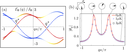
Figure 2: (Color online) (a) SOC band structure for $\delta=-2J_{\mathbf{0}}$, $\Omega_{\mathbf{0}}=J_{\mathbf{0}}$ (solid lines) and $\Omega_{\mathbf{0}}^{p}=0.05J_{\mathbf{0}}$ (dashed lines). The axial depth is $V/E_{R}=12$, $J_{\mathbf{0}}=42$ Hz and $h\nu_{\perp}\approx 900$ Hz. Colors correspond to state character, with $g$ ($e$) being more blue (red). (b) Chiral Bloch vector angle, $\theta_{\mathbf{0}q}$, in the $xz$ plane extracted from Rabi spectroscopy using the protocol explained in the text Supp . The figure shows three temperatures for the parameters of (a).

The ability to resolve the $q^{\star}_{\mathbf{n}}$ resonances that appear across the entire Brillouin zone (BZ) as the detuning is varied can be used to perform momentum resolved spectroscopy and to precisely determine the chiral Bloch vector angle $\theta_{\mathbf{0}q}$ for given values of $\Omega_{\mathbf{0}}$ and $\delta$ from Rabi oscillations. We propose the use of a three spectroscopic sequences Supp . One sequence selectively excites atoms at $q^{\star}_{\mathbf{n}}$ from $g$ to $e$ and induces Rabi oscillations. Another filters the dynamics of the excited atoms from the remaining $g$ atoms and the third is used to “correct” imperfections arising from finite temperature. As shown in Fig. 2(b), this protocol allows us to extract $\theta_{\mathbf{0}q}$ over the BZ. This method is not restricted to OLCs, requiring only a stable probe, and complements other techniques for measuring band structures Tarruell ; Atala ; Duca used in degenerate Fermi gases.

Ramsey spectroscopy The standard Ramsey protocol starts with all atoms in the $g$ state and subjects them to two strong, near-resonant laser pulses separated by a free evolution “dark” time $\tau$. The first pulse rotates the Bloch vector by an angle $\theta_{1}$ set by the pulse area, and the second converts the accumulated phase during the dark time into a $g-e$ population difference measured as Ramsey fringes. Interactions induce a density-dependent frequency shift in the fringes.

Interactions between two nuclear spin polarized atoms depend on the motional and electronic degrees of freedom Rey_Annals . When the atoms collide they experience $s$-wave interactions, characterized by the elastic scattering length $a_{eg}$, when their electronic state is antisymmetric $(|eg\rangle-|ge\rangle)/\sqrt{2}$. They can also collide via $p$-wave interactions, described by the corresponding $p$-wave elastic scattering volumes $b_{gg}^{3}$, $b_{ee}^{3}$, and $b_{eg}^{3}$, in the three possible symmetric electronic configurations $|gg\rangle,|ee\rangle,(|eg\rangle+|ge\rangle)/\sqrt{2}$, respectively. In addition to elastic interactions, atoms can also exhibit inelastic collisions. In ⁸⁷Sr only the $ee$ type has been observed to give rise to measurable losses SUN2 while in ^173,171 Yb, both $ee$ and $eg$ losses have been reported losses1 ; losses2 ; Scazza . The effect of losses can be compensated by tracking the population decay during the dark time Martin_2013 ; lemke2011 .

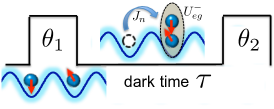
Figure 3: (Color online) A clock laser pulse with pulse area $\theta_{1}$ imprints a phase difference $\phi$ between atoms in neighboring sites. Atom tunneling, $J_{\mathbf{n}}$, allows for $s$-wave interactions, $\propto U_{eg}^{-}$, which are signaled as a density shift in Ramsey spectroscopy after a second pulse of area $\theta_{2}$ is applied.

When tunneling is suppressed the differential phase imparted by the laser is irrelevant, and as long as $\Omega_{\mathbf{n}}$ is the same for all modes – a condition well-satisfied in current OLCs Martin_2013 – the collective spin of the atoms within each lattice site remains fully symmetric after the pulse and only $p$-wave collisions occur during the dark time. Measurements under this condition  Martin_2013 ; lemke2011 indeed observed a frequency shift linearly dependent on the excitation fraction of atoms, $(1-\cos\theta_{1})/2$ and fully consistent with a $p$-wave interacting model Rey_Annals . If instead tunneling is allowed during the dark time, atoms become sensitive to the spatially inhomogeneous spin rotation from the site-dependent laser phase, which in turn allows for $s$-wave collisions after a tunneling event (see Fig. 3). The $s$-wave collisions in SOC-coupled spin polarized fermions can lead to exotic phases of matter including topological quantum liquids ZhangTewari ; Julia-Diaz .

In typical OLCs the interaction energy per particle (at the Hz level) is weaker than the vibrational energy spacing, and large anharmonicity prevents resonant interaction-induced mode transverse changes, and so a description in terms of fixed transverse motional levels is justified Rey_Annals . In the regime of weak interactions compared to tunneling, we compute the dynamics perturbatively, and find that SOC manifests itself in the density shift at short times as Supp

$$\Delta\nu =\Delta\nu_{0}\left[1+\frac{4\langle{J^{2}}\rangle_{T_{R}}\tau^{2}{\zeta}\cos\theta_{1}\sin^{2}\frac{\phi}{2}}{3\hbar^{2}({C}-{\chi}\cos\theta_{1})}\right]\,,$$ (4)

where $\Delta\nu_{0}=N(C-\chi\cos\theta_{1})$ is the density shift in the absence of tunneling Martin_2013 ; Rey_Annals , $N$ the mean atom number per pancake, $\langle J^{2}\rangle_{T_{R}}$ the thermally averaged squared tunneling rate, $\zeta=\left(V^{eg}-U^{eg}\right)/2$, $\chi=(V^{ee}+V^{gg}-2V^{ge})/{2}$, and $C=(V^{ee}-V^{gg})/{2}$, with $V^{\alpha\alpha^{\prime}}=b_{\alpha\alpha^{\prime}}^{3}\langle P\rangle_{T_{R}}$ and $U^{eg}=a^{−}_{eg}\langle S\rangle_{T_{R}}$.Here $\langle P\rangle_{T_{R}}\propto(T_{R})^{0}$ and $\langle S\rangle_{T_{R}}\propto T_{R}^{-1}$ correspond to the thermal averages of the $p$-wave and $s$-wave mode overlap coefficients respectively Rey_Annals , and $T_{R}$ is the radial temperature. For the JILA ⁸⁷Sr clock operated at $T_{R}\sim(1-5)\mu$K and $\theta_{1}\ll\pi$ for $\tau\sim 80$ ms, $\Delta\nu_{0}\sim-5$Hz. Here, $E_{R}$ is the recoil energy. Since SOC introduces contributions from $s$-wave interactions, which can be one order of magnitude larger than $p-$wave at $T_{R}\sim 1\mu$K, then from Eq. 4 we expect significant modifications of the density shift.

Sliding Superlattice: We consider the third case where the interrogation is done by a pair of counter-propagating beams close to resonance with the clock transition and with a global phase difference $\Upsilon(t)$ which can be controlled in time (see Fig. 4(a)). The non-interacting Hamiltonian, written using a Wannier orbital basis along the lattice direction, is

$$\hat{H}_{L}^{0}=-\sum_{\mathbf{n},j,\alpha}\left(J_{\mathbf{n}}\left[\hat{a}^{\dagger}_{\alpha,\mathbf{n},j}\hat{a}_{\alpha,\mathbf{n},j+1}+\mathrm{H.c.}\right]-\frac{\delta}{2}\alpha\hat{n}_{\alpha\mathbf{n},j}\right)$$

$$-\sum_{\mathbf{n},j}\left(\Omega_{\mathbf{n}}\cos(\Upsilon(t)-j\phi)\left[\hat{a}^{\dagger}_{+,\mathbf{n},j}\hat{a}_{-,\mathbf{n},j}+\mathrm{H.c.}\right]\right).$$ (5)

As $\Upsilon(t)$ is changed, the clock laser standing wave “slides” with respect to the optical lattice. This allows for the minimum realization of a topological pump when $\Upsilon(t)$ is adiabatically varied from $0\to 2\pi$ Thouless ; TroyerPump ; KwekPump ; MuellerPump ; CooperRey . In the weak tunneling limit the quantized nature of particle transport can be directly linked to spatially isolated tunneling resonances  CooperRey . We now show how those resonances can be spectroscopically measured in OLCs.

Let us first consider the case $J_{\mathbf{n}}=\delta=0$ and set $\phi=7\pi/6$, relevant for the ⁸⁷Sr system. We write $\Upsilon=(2\pi s+\Delta\Upsilon)/12$, with $0\leq\Delta\Upsilon<2\pi$ and $s$ an integer. Under these conditions, the localized dressed eigenstates are spin-polarized along $\pm x$ alternating between neighboring sites except for “defects” at $j_{d}(r)=6r+3+s$ ($r$ an integer) when $\cos(\Upsilon-\Delta\Upsilon/12-j_{d}\phi)=0$ and the ground states at $j_{d}(r)$ and $j_{d}(r)+1$ point along the same direction. Since tunneling preserves polarization, it is suppressed when $J_{\mathbf{n}}\ll\Omega_{\mathbf{n}}$ due to the energy offset $\sim\Omega$ between neighboring sites. The one exception is the case $\Delta\Upsilon=\pi$ where the defect pair $j_{d}(r)$ and $j_{d}(r)+1$ is resonantly tunnel-coupled. Quantized transport occurs when $\Delta\Upsilon$ is slowly varied across the resonance. Instead of adiabatic transport we propose to spectroscopically resolve the resonance using a Ramsey-type protocol. Here, atoms initially prepared in $g$ at $|\delta|\gg\Omega_{\mathbf{0}}$ are adiabatically transferred to the ground dressed state by slowly turning off $\delta$ at $\Upsilon=(2\pi s+\Delta\Upsilon_{p})/12$ with $\Delta\Upsilon_{p}\neq\pi$. Then $\Upsilon$ is quenched so resonant tunneling is allowed, $s\to s+1$ and $\Delta\Upsilon=\pi$, and the system evolves for a time $\tau$. Following this evolution tunneling is turned off and the phase switched back, $s+1\to s$ and $\Delta\Upsilon\to\Delta\Upsilon_{p}$. Those atoms which have tunneled at the resonant sites are now in an excited state of the local dressed basis. These excitations can be measured by adiabatically converting the dressed excitations to “bare” $e$ excitations by adiabatically ramping on $\delta\gg\Omega_{\mathbf{0}}$; this leads to a measurable excited state population $n_{e}(t)$. In Fig. 4(c) we show these tunneling resonances are clearly observable even at finite temperature. Moreover, since resonances are spatially well-separated (every six sites), they can be resolved with low-resolution imaging.

Interactions modify the transport dynamics in our protocol. The sliding superlattice simplifies the treatment of interactions by isolating resonant site pairs $\{j_{d},j_{d}+1\}$. We consider the case where at most two atoms occupy the resonant sites, a condition which can be achieved by decreasing the atomic density with a large-volume dipole trap Bloom . The two particle states can be classified in terms of the atoms’ spin polarization along $x$ in four sectors: three symmetric ones (triplets) with total $x$ polarization $M_{x}=+1,-1,0$ and a $M_{x}=0$ singlet. Within each sector, the dressed states’ interaction parameters are given by Supp $V_{+1}=V_{-1}=(V^{gg}+V^{ee}+2V^{eg})/4$, $V_{0}=(V^{gg}+V^{ee})/2$ and $U_{0}=U^{eg}$ (see Fig. 4(b)). Since the $p$-wave parameters are not SU$(2)$ symmetric, i.e. $b_{ee}\neq b_{gg}\neq b_{eg}$, the triplet sectors are coupled. However, in the weakly interacting limit $V^{\alpha\beta}\ll\Omega$, the triplets are separated by energy gaps $\sim\Omega$ and coupling between the sectors can be neglected. The singlet sector is always decoupled from the triplets.

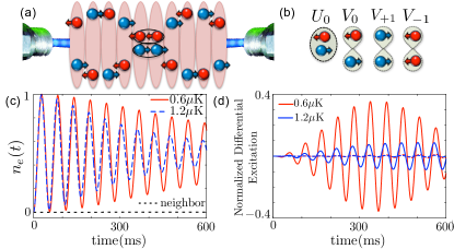
Figure 4: (a) An additional counter-propagating probing beam with a differential phase $\Upsilon$ generates a sliding superlattice potential, shown for $\phi=7\pi/6$, corresponding to an ⁸⁷Sr OLC. For weak tunneling $J\ll\Omega$ transport is energetically suppressed except at resonant defect points (circled). (b) Two-particle interaction sectors classified by the total polarization $M_{x}$ and spatial symmetry of the dressed states. An oval (figure-eight) denotes a symmetric (antisymmetric) spatial wavefunction. (c) Dynamics of a single particle at the tunneling resonance for two temperatures (red solid and blue dashed) and an off-resonant site (black dotted) for $J_{\mathbf{0}}=8$Hz, $\Omega_{\mathbf{0}}=1$kHz, $\phi=7\pi/6$. (d) Normalized differential excitation extracted as explained in the text with the interaction parameters of Ref. SUN2 . The $M_{x}=0$ components (solid lines) involve the $s$-wave sector, and so display a strong dependence of contrast on temperature, while the $M_{\pm 1}$ sectors (dashed lines) experience only weaker single-particle thermal dephasing.

Within each sector interactions modify the dynamics making it sensitive to temperature and density. The modifications can be extracted by performing measurements of the atom number-normalized excitation fraction for different densities and then differentiating the high-density and low-density results Supp . This procedure removes the single-particle contribution and is particularly suitable for characterizing the role of interactions in clock experiments Martin_2013 ; SUN2 . The normalized differential excitation is shown in Fig. 4(d). For the adiabatic dressed state preparation, all four manifolds, and hence all interaction parameters $V_{\pm,0},U_{0}$, contribute to the dynamics. A filtering protocol that uses the $ee$ losses can be used to separate the dynamics of the various sectors. For example, by transferring all atoms to the $e$ state and holding before the adiabatic ground state preparation, the doubly occupied $M_{x}=\pm 1$ triplet sectors will be removed and only the $M_{x}=0$ singlet and triplet remain and contribute (here the ground dressed states have one atom at $j_{d}$ and $j_{d}+1$). As shown in Fig. 4 the dynamics of the $V_{\pm,0}$ and $U_{0}$ sectors can be distinguished by the different scaling of the $p$ and $s$-wave interaction parameters with temperature $T_{R}$, $V_{\pm,0}\left(T_{R}\right)\sim\mathrm{const.}$ and $U_{0}\left(T_{R}\right)\sim T_{R}^{-1}$ Rey_Annals (See Fig.4(d)). By comparing these dynamics to that without the holding time, information about the $M_{x}=\pm 1$ dynamics can be extracted. In general $s$-wave interactions dominate the normalized differential contrast, with $p$-wave contributions relevant only at hotter temperatures.

Summary We have described approaches to implement and probe SOC in OLCs. We showed the proposed protocols provide clean signatures of SOC in interacting many-body systems. While they work at the temperatures achievable in current OLCs, their sensitivity and applicability are expected to significantly improve when operating the clock in the quantum degenerate regime. Moreover, if nuclear spins are included, they can open a window for the investigation of SOC with SU(N)-symmetric collisions Cazalilla_rev .

Acknowledgments We thank Ed Marti and James Thompson for comments on the manuscript, and Leonid Isaev and the JILA Sr clock team for discussions. This work was supported by the NSF (PIF-1211914 and PFC-1125844), AFOSR, AFOSR-MURI, NIST and ARO, the EPSRC Grant EP/K030094/1, and by the JILA Visiting Fellows Program. MLW thanks the NRC postdoctoral fellowship program for support. AK was supported by the Department of Defense through the NDSEG program.

Supplemental Material for “Exploring synthetic spin-orbit coupling in a thermal optical lattice clock”

Interaction Hamiltonian with the spin model assumption The Hamiltonian governing fermionic AEAs in an optical lattice clock may be written:

$$\hat{H} =\hat{H}_{0}+\hat{H}_{I}+\hat{H}_{L}\,,$$ (S1)

$$\hat{H}_{0} =\sum_{\alpha}\int d\mathbf{r}\hat{\psi}_{\alpha}\left(\mathbf{r}\right)\left[-\frac{\hbar^{2}}{2m}\nabla^{2}+V_{\mathrm{ext}}\left(\mathbf{r}\right)\right]\hat{\psi}_{\alpha}\left(\mathbf{r}\right)-\hbar\delta\int d\mathbf{r}\hat{\psi}_{e}^{\dagger}\left(\mathbf{r}\right)\hat{\psi}_{e}\left(\mathbf{r}\right)\,,$$ (S2)

$$\hat{H}_{I} =\frac{4\pi\hbar^{2}a_{eg}^{-}}{m}\int d\mathbf{r}\hat{\psi}_{e}^{\dagger}\left(\mathbf{r}\right)\hat{\psi}_{e}\left(\mathbf{r}\right)\hat{\psi}_{g}^{\dagger}\left(\mathbf{r}\right)\hat{\psi}_{g}\left(\mathbf{r}\right)+\sum_{\alpha\beta}\frac{3\pi\hbar^{2}b^{3}_{\alpha\beta}}{m}\int d\mathbf{r}W\left[\hat{\psi}^{\dagger}_{\alpha}(\mathbf{r}),\hat{\psi}^{\dagger}_{\beta}(\mathbf{r})\right]\left(W\left[\hat{\psi}^{\dagger}_{\alpha}(\mathbf{r}),\hat{\psi}^{\dagger}_{\beta}(\mathbf{r})\right]\right)^{\dagger}\,,$$ (S3)

$$\hat{H}_{L} =-\frac{\hbar\Omega}{2}\int d\mathbf{r}\left[\hat{\psi}_{e}^{\dagger}\left(\mathbf{r}\right)e^{i2\pi Z/\lambda}\hat{\psi}_{g}\left(\mathbf{r}\right)+\mathrm{H.c.}\right]$$ (S4)

where $m$ is the atomic mass, $\hat{\psi}_{\alpha}\left(\mathbf{r}\right)$ is a fermionic field operator for state $\alpha\in\left\{g,e\right\}$, $W\left[\hat{A}\left(\mathbf{r}\right),\hat{B}\left(\mathbf{r}\right)\right]=(\nabla\hat{A}\left(\mathbf{r}\right))\hat{B}\left(\mathbf{r}\right)-\hat{A}\left(\mathbf{r}\right)(\nabla\hat{B}\left(\mathbf{r}\right))$ is the Wronskian, and $\delta=\omega_{l}-\omega_{0}$ is the difference between the clock laser frequency $\omega_{l}$ and atomic frequency $\omega_{0}$ in the rotating frame of the laser. The Hamiltonian $\hat{H}_{0}$ contains the kinetic energy and trapping potential $V_{\mathrm{ext}}\left(\mathbf{r}\right)$, $\hat{H}_{I}$ contains the effects of $s$-wave interactions with scattering length $a_{eg}^{-}$ and $p$-wave interactions with interaction volumes $b_{\alpha\beta}^{3}$ between nuclear spin-polarized AEAs, and $\hat{H}_{L}$ describes the coupling of internal levels to the clock laser. We assume that the optical lattice is deep enough that we can neglect interactions occurring between different lattice sites, and so consider only interactions between particles occupying the same lattice site. Further, we enact the spin model approximation Rey_Annals , which neglects all interactions which do not preserve the single-particle transverse mode occupations during a two-body collision. The spin model Hamiltonian hence keeps only direct terms, in which the two colliding particles remain in their same transverse motional quantum states, and exchange processes where the transverse quantum numbers of the two colliding particles are exchanged. The spin model Hamiltonian is valid when interactions are smaller than the spacing between transverse modes, and also when anharmonicity of the potential prevents collisional exchange of mode energy between transverse dimensions.

To derive a Hubbard model amenable for direct calculation, we expand the field operators in a basis of single-particle eigenfunctions. In order to facilitate thermal averages, we take this set of functions to be the eigenfunctions of $\hat{H}_{0}$, $\psi_{q,n}\left(\mathbf{r}\right)$, which are indexed in terms of a quasimomentum $q$ and a transverse mode index $\mathbf{n}$. Enacting this expansion with the approximations of the last paragraph, we find

$$\hat{H}_{I} =\frac{1}{4L}\sum_{\alpha\beta}\sum_{\left\{\mathbf{n}_{1},\mathbf{n}_{2}\right\}}\sum_{qq^{\prime}\Delta q}\Big{[}\left(2-\delta_{\mathbf{n}_{1}\mathbf{n}_{2}}\right)\left(U^{\alpha\beta}_{\left\{\mathbf{n}_{1},\mathbf{n}_{2}\right\}}+V^{\alpha\beta}_{\left\{\mathbf{n}_{1},\mathbf{n}_{2}\right\}}\right)\hat{a}^{\dagger}_{\alpha,q+\Delta q,\mathbf{n}_{1}}\hat{a}^{\dagger}_{\beta,q^{\prime}-\Delta q,\mathbf{n}_{2}}\hat{a}_{\beta,q^{\prime},\mathbf{n}_{2}}\hat{a}_{\alpha,q,\mathbf{n}_{1}}$$

$$+2\left(1-\delta_{\mathbf{n}_{1}\mathbf{n}_{2}}\right)\left(V^{\alpha\beta}_{\left\{\mathbf{n}_{1},\mathbf{n}_{2}\right\}}-U^{\alpha\beta}_{\left\{\mathbf{n}_{1},\mathbf{n}_{2}\right\}}\right)\hat{a}^{\dagger}_{\beta,q^{\prime}-\Delta q,\mathbf{n}_{1}}\hat{a}^{\dagger}_{\alpha,q+\Delta q,\mathbf{n}_{2}}\hat{a}_{\beta,q^{\prime},\mathbf{n}_{2}}\hat{a}_{\alpha,q,\mathbf{n}_{1}}\Big{]}\,.$$ (S5)

Here, $L$ is the number of lattice sites, the sum over $\left\{\mathbf{n}_{1},\mathbf{n}_{2}\right\}$ means the sum over distinct, ordered pairs of transverse modes, $q$, $q^{\prime}$, and $\Delta q$ are quasimomenta in the first Brillouin zone (BZ), greek letters denote internal electronic states $\alpha,\beta\in\left\{g,e\right\}$, and the interaction matrix elements may be written as

$$U^{\alpha\beta}_{\left\{\mathbf{n}_{1},\mathbf{n}_{2}\right\}} =\left(1-\delta_{\alpha\beta}\right)\frac{8\pi\hbar^{2}}{m}a_{s}S_{\mathbf{n}_{1}\mathbf{n}_{2}\mathbf{n}_{2}\mathbf{n}_{1}}\,,\;\;V^{\alpha\beta}_{\left\{\mathbf{n}_{1},\mathbf{n}_{2}\right\}}=\frac{12\pi\hbar^{2}}{m}b^{3}_{\alpha\beta}P_{\mathbf{n}_{1}\mathbf{n}_{2}\mathbf{n}_{2}\mathbf{n}_{1}}$$ (S6)

by defining the integrals

$$S_{\mathbf{n}_{1}^{\prime}\mathbf{n}_{2}^{\prime}\mathbf{n}_{2}\mathbf{n}_{1}} =\int d\mathbf{r}\psi_{i,\mathbf{n}_{1}^{\prime}}^{\star}\left(\mathbf{r}\right)\psi_{i,\mathbf{n}_{2}^{\prime}}^{\star}\left(\mathbf{r}\right)\psi_{i,\mathbf{n}_{2}}\left(\mathbf{r}\right)\psi_{i,\mathbf{n}_{1}}\left(\mathbf{r}\right)\,,\;\;P_{\mathbf{n}_{1}^{\prime}\mathbf{n}_{2}^{\prime}\mathbf{n}_{2}\mathbf{n}_{1}}=\int d\mathbf{r}W\left[\psi^{\star}_{i,\mathbf{n}_{1}^{\prime}}\left(\mathbf{r}\right),\psi^{\star}_{i,\mathbf{n}_{2}^{\prime}}\left(\mathbf{r}\right)\right]W\left[\psi_{i,\mathbf{n}_{1}}\left(\mathbf{r}\right),\psi_{i,\mathbf{n}_{2}}\left(\mathbf{r}\right)\right]\,.$$ (S7)

In the latter two expressions, the wavefunctions are localized Wannier-type functions obtained from the quasimomentum-indexed eigensolutions (Bloch functions) of the full 3D potential as $\psi_{j,\mathbf{n}}\left(\mathbf{r}\right)=\frac{1}{\sqrt{L}}\sum_{q\in\mathrm{BZ}}e^{-iqr_{j}}\psi_{q,\mathbf{n}}\left(\mathbf{r}\right)$ Wall_Hazzard_15 . We can also define the mode-dependent tunneling and Rabi frequency in terms of these functions as

$$J_{\mathbf{n}} =-\int d\mathbf{r}\psi_{j,\mathbf{n}}\left(\mathbf{r}\right)\left[-\frac{\hbar^{2}}{2m}\nabla^{2}+V_{\mathrm{ext}}\left(\mathbf{r}\right)\right]\psi_{j+1,\mathbf{n}}\left(\mathbf{r}\right)\,,$$ (S8)

$$\Omega_{\mathbf{n}} =\Omega\int d\mathbf{r}\psi_{j,\mathbf{n}}\left(\mathbf{r}\right)e^{i2\pi Z/\lambda}\psi_{j,\mathbf{n}}\left(\mathbf{r}\right)\,.$$ (S9)

First-order density shift in Ramsey spectroscopy In this section we compute the density shift for Ramsey spectroscopy to first order in interactions using an interaction picture perturbation series. In particular, we write the propagator during the dark time evolution in terms of a truncated Dyson series $e^{-i\hat{H}t}=e^{-i\hat{H}_{0}t}-i\int_{0}^{t}dt^{\prime}e^{-i\hat{H}_{0}\left(t-t^{\prime}\right)}\hat{H}_{1}e^{-i\hat{H}_{0}t^{\prime}}.$ At the end of the dark time, a spin-rotation pulse of area $\theta_{2}$ is applied, and then the total $\hat{S}^{z}$ is measured. These two operations can be combined as the measurement of the operator $\hat{S}^{z}_{\theta}=\sum_{nq}\left[\cos\theta\hat{S}^{z}_{q\mathbf{n}}-\sin\theta\hat{S}^{y}_{q\mathbf{n}}\right]$. Hence, the first-order result of the Ramsey sequence is

$$\langle\hat{S}^{z}\left(\tau\right)\rangle=\langle\psi\left(\theta_{1}\right)|e^{i\hat{H}_{0}\tau}\hat{S}^{z}_{\theta_{2}}e^{-i\hat{H}_{0}\tau}|\psi\left(\theta_{1}\right)\rangle+2\mathcal{I}\left[\langle\psi\left(\theta_{1}\right)|e^{i\hat{H}_{0}\tau}\hat{S}^{z}_{\theta_{2}}\int_{0}^{\tau}dte^{-i\hat{H}_{0}\left(\tau-t\right)}\hat{H}_{I}e^{-i\hat{H}_{0}t}|\psi\left(\theta_{1}\right)\rangle\right]\,,$$ (S10)

where $|\psi\left(\theta_{1}\right)\rangle$ is the state resulting from applying the first Ramsey pulse to an initial state $|\tilde{i}\rangle$. We will parameterize the initial state in terms of products of single-particle eigenstates $|i\rangle=\prod_{i=1}^{N}\hat{a}^{\dagger}_{gq_{i}n_{i}}|\mathrm{vac.}\rangle$, where $|\mathrm{vac}.\rangle$ is the vacuum, $N$ the number of particles, and $\left\{q_{i},\mathbf{n}_{i}\right\}$ the initial distinct set of populated quasimomenta and transverse modes, so that

$$|\psi\left(\theta_{1}\right)\rangle =\prod_{j=1}^{N}\left(\cos\frac{\theta_{1}}{2}\hat{a}^{\dagger}_{g,q_{j},\mathbf{n}_{j}}+i\sin\frac{\theta_{1}}{2}\hat{a}^{\dagger}_{e,q_{j},\mathbf{n}_{j}}\right)\,.$$ (S11)

From this, we find that the non-interacting dynamics are given as

$$\langle\psi\left(\theta_{1}\right)|e^{i\hat{H}_{0}\tau}\hat{S}^{z}_{\theta_{2}}e^{-i\hat{H}_{0}\tau}|\psi\left(\theta_{1}\right)\rangle=\sum_{i=1}^{N}\left[-\frac{\cos\theta_{1}\cos\theta_{2}}{2}+\frac{\sin\theta_{1}\sin\theta_{2}}{2}\cos\left(\delta\tau-\Delta E_{\mathbf{n}_{i}}\left(q_{i},\phi\right)\tau\right)\right]\,,$$ (S12)

where $E_{\mathbf{n}}\left(q\right)$ is the single-particle dispersion and

$$\Delta E_{\mathbf{n}}\left(q,\phi\right)\equiv E_{\mathbf{n}}\left(q+\phi\right)-E_{\mathbf{n}}\left(q\right)\,,$$ (S13)

is the difference in single-particle dispersion of the $e$ and $g$ states.

Writing the non-interacting result as $\langle\hat{S}^{z}\left(\tau\right)\rangle=A\left(\tau\right)\cos\left(\delta\tau\right)+B\left(\tau\right)\sin\left(\delta\tau\right)+\mathrm{const.}$ we can extract the density shift as $\Delta\nu=\frac{1}{2\pi\tau}\mathrm{arctan}\left(\frac{B\left(\tau\right)}{A\left(\tau\right)}\right)$ and the normalized contrast decay as $\mathcal{C}\left(\tau\right)=\frac{\sqrt{A^{2}\left(\tau\right)+B^{2}\left(\tau\right)}}{\sqrt{A^{2}\left(0\right)+B^{2}\left(0\right)}}\,.$ For a single particle with momentum $q$ and transverse mode $n$, the density shift is $\Delta E_{\mathbf{n}}\left(q,\phi\right)/2\pi$. Assuming short times compared to the tunneling bandwidth, the density shifts for all particles add as $\Delta\nu=\sum_{i=1}^{N}\Delta E_{\mathbf{n}_{i}}\left(q_{i},\phi\right)/2\pi N+\mathcal{O}\left(\tau^{2}\right)$. The contrast decay at short times is given as $\mathcal{C}\left(\tau\right)=1-\frac{1}{2N^{2}}\left(\sum_{i=1}^{N}\Delta E_{\mathbf{n}_{i}}\left(q_{i},\phi\right)\right)^{2}\tau^{2}+\frac{1}{2N}\sum_{i=1}^{N}\Delta E_{\mathbf{n}_{i}}^{2}\left(q_{i},\phi\right)\tau^{2}+\mathcal{O}\left(\tau^{4}\right)$. This single-particle contribution will dominate over the $\sim U^{2}\tau^{2}$ decay of the contrast due to interactions at short times and in the regime of weak interactions compared to the tunneling.

The contribution to the dynamics at the lowest order in interactions is given as

$$2\mathcal{I}\left[\langle\psi\left(\theta_{1}\right)|e^{i\hat{H}_{0}\tau}\hat{S}^{z}_{\theta_{2}}\int_{0}^{\tau}dte^{-i\hat{H}_{0}\left(\tau-t\right)}\hat{H}_{I}e^{-i\hat{H}_{0}t}|\psi\left(\theta_{1}\right)\rangle\right]$$ (S14)

$$=\frac{\tau}{L}\sum_{\left\{p_{1},p_{2}\right\}}\Big{\{}\sin\theta_{1}\sin\theta_{2}\sin\left[\left(\delta-\frac{\Delta E_{\mathbf{n}_{p_{1}}}\left(q_{p_{1}},\phi\right)+\Delta E_{\mathbf{n}_{p_{2}}}\left(q_{p_{2}},\phi\right)missing}{2}\right)\tau\right]$$

$$\times\Big{[}\left(C_{\left\{\mathbf{n}_{p_{1}}\mathbf{n}_{p_{2}}\right\}}-\chi_{\left\{\mathbf{n}_{p_{1}}\mathbf{n}_{p_{2}}\right\}}\cos\theta_{1}\right)\cos\left(\frac{\Delta E_{\mathbf{n}_{p_{1}}}\left(q_{p_{1}},\phi\right)-\Delta E_{\mathbf{n}_{p_{2}}}\left(q_{p_{2}},\phi\right)missing}{2}\tau\right)$$

$$-\frac{\cos\theta_{1}}{2}\left(2-\delta_{\mathbf{n}_{p_{1}}\mathbf{n}_{p_{2}}}\right)\zeta_{\left\{\mathbf{n}_{p_{1}}\mathbf{n}_{p_{2}}\right\}}\Big{[}\cos\left(\frac{\Delta E_{\mathbf{n}_{p_{1}}}\left(q_{p_{1}},\phi\right)-\Delta E_{\mathbf{n}_{p_{2}}}\left(q_{p_{2}},\phi\right)missing}{2}\tau\right)-\mathrm{sinc}\left(\frac{\Delta E_{\mathbf{n}_{p_{1}}}\left(q_{p_{1}},\phi\right)-\Delta E_{\mathbf{n}_{p_{2}}}\left(q_{p_{2}},\phi\right)missing}{2}\tau\right)\Big{]}\Big{]}\Big{\}}$$

where the mode-dependent spin model parameters are

$$C_{\left\{\mathbf{n}_{1}\mathbf{n}_{2}\right\}} =\frac{V^{ee}_{\{\mathbf{n}_{1}\mathbf{n}_{2}\}}-V^{gg}_{\{\mathbf{n}_{1}\mathbf{n}_{2}\}}}{2}$$ (S15)

$$\chi_{\left\{\mathbf{n}_{1}\mathbf{n}_{2}\right\}} =\frac{V^{ee}_{\{\mathbf{n}_{1}\mathbf{n}_{2}\}}+V^{gg}_{\{\mathbf{n}_{1}\mathbf{n}_{2}\}}-2V^{ge}_{\{\mathbf{n}_{1}\mathbf{n}_{2}\}}}{2}$$ (S16)

$$\zeta_{\left\{\mathbf{n}_{1}\mathbf{n}_{2}\right\}} =\frac{V^{eg}_{\{\mathbf{n}_{1}\mathbf{n}_{2}\}}-U^{ge}_{\{\mathbf{n}_{1}\mathbf{n}_{2}\}}}{2}\,.$$ (S17)

Taking a series in the tunneling bandwidth, the zeroth order term for a given pair of particles is $\left(C-\chi\cos\theta_{1}\right)\sin\theta_{1}\sin\theta_{2}\sin\delta\tau$, which has been obtained in previous works Martin_2013 . The thermally averaged density shift in the high-temperature limit will be given in the next section.

High-temperature thermal average of density shift Here, we derive the high-temperature (compared to the tunneling bandwidth) thermal average of the first-order many-body dynamics derived in the last section. First, we expand the above result to third order in time, finding

$$\langle\hat{S}^{z}\left(\tau\right)\rangle =\frac{1}{2}\sum_{i=1}^{N}\left(\cos\left(\delta\tau\right)\sin\theta_{1}\sin\theta_{2}-\cos\theta_{1}\cos\theta_{2}\right)$$ (S18)

$$+\sum_{\left\{p_{1},p_{2}\right\}}\frac{\sin\theta_{1}\sin\theta_{2}}{L}\tau\left(C_{\left\{\mathbf{n}_{p_{1}},\mathbf{n}_{p_{2}}\right\}}-\chi_{\left\{\mathbf{n}_{p_{1}},\mathbf{n}_{p_{2}}\right\}}\cos\theta_{1}\right)\sin\delta\tau+\frac{1}{2}\sum_{i=1}^{N}\Delta E_{\mathbf{n}_{i}}\left(q_{i},\phi\right)\sin\left(\delta\tau\right)\sin\theta_{1}\sin\theta_{2}\tau$$

$$-\sum_{\left\{p_{1},p_{2}\right\}}\frac{\sin\theta_{1}\sin\theta_{2}}{L}\frac{\tau^{2}}{2}\left(C_{\left\{\mathbf{n}_{p_{1}},\mathbf{n}_{p_{2}}\right\}}-\chi_{\left\{\mathbf{n}_{p_{1}},\mathbf{n}_{p_{2}}\right\}}\cos\theta_{1}\right)\left(\Delta E_{\mathbf{n}_{p_{1}}}\left(q_{p_{1}},\phi\right)+\Delta E_{\mathbf{n}_{p_{2}}}\left(q_{p_{2}},\phi\right)\right)\cos\delta\tau$$

$$-\frac{1}{4}\sum_{i=1}^{N}\Delta E_{\mathbf{n}_{i}}\left(q_{i},\phi\right)^{2}\cos\left(\delta\tau\right)\sin\theta_{1}\sin\theta_{2}\tau^{2}$$

$$-\sum_{\left\{p_{1},p_{2}\right\}}\frac{\sin\theta_{1}\sin\theta_{2}}{L}\frac{\tau^{3}}{24}\Big{[}6\left(C_{\left\{\mathbf{n}_{p_{1}},\mathbf{n}_{p_{2}}\right\}}-\chi_{\left\{\mathbf{n}_{p_{1}},\mathbf{n}_{p_{2}}\right\}}\cos\theta_{1}\right)\left(\Delta E_{\mathbf{n}_{p_{1}}}\left(q_{p_{1}},\phi\right)^{2}+\Delta E_{\mathbf{n}_{p_{2}}}\left(q_{p_{2}},\phi\right)^{2}\right)$$

$$-\left(2-\delta_{\mathbf{n}_{p_{1}}\mathbf{n}_{p_{2}}}\right)\zeta_{\left\{\mathbf{n}_{p_{1}},\mathbf{n}_{p_{2}}\right\}}\left(\Delta E_{\mathbf{n}_{p_{1}}}\left(q_{p_{1}},\phi\right)-\Delta E_{\mathbf{n}_{p_{2}}}\left(q_{p_{2}},\phi\right)\right)^{2}\cos\theta_{1}\sin\delta\tau\Big{]}$$

$$-\frac{1}{12}\sum_{i=1}^{N}\Delta E_{\mathbf{n}_{i}}\left(q_{i},\phi\right)^{3}\sin\left(\delta\tau\right)\sin\theta_{1}\sin\theta_{2}\tau^{3}\Big{\}}\,.$$

To perform thermal averages, we now enact the tight-binding approximation, in which $E_{\mathbf{n}}\left(q\right)=\bar{E}_{\mathbf{n}}-2J_{\mathbf{n}}\cos\left(q\right)$, and compute the partition function as

$$Z =\sum_{nq}e^{-\beta E_{\mathbf{n}}\left(q\right)}\approx\sum_{\mathbf{n}}e^{-\beta\bar{E}_{\mathbf{n}}}\int_{-1}^{1}dqe^{2\beta J_{\mathbf{n}}\cos\left(\pi q\right)}$$ (S19)

$$=2\sum_{\mathbf{n}}e^{-\beta\bar{E}_{\mathbf{n}}}I_{0}\left(2\beta J_{\mathbf{n}}\right)=2\sum_{\mathbf{n}}e^{-\beta\bar{E}_{\mathbf{n}}}\left[1+\mathcal{O}\left(\beta^{2}J_{\mathbf{n}}^{2}\right)\right]\,,$$ (S20)

where $I_{\nu}\left(x\right)$ is the modified Bessel function of order $\nu$ and $\beta$ the inverse radial temperature. Hence, for temperatures sufficiently high compared to the bandwidth $J_{\mathbf{n}}$, the partition function is just a constant times the partition function of the transverse modes. Now,

$$\langle\Delta E_{n}\left(q,\phi\right)\rangle_{T_{R}} =\frac{1}{Z}\sum_{\mathbf{n}}e^{-\beta\bar{E}_{\mathbf{n}}}4J_{\mathbf{n}}\left(1-\cos\phi\right)I_{1}\left(2\beta J_{\mathbf{n}}\right)$$ (S21)

$$=\frac{1}{Z_{\mathbf{n}}}\sum_{\mathbf{n}}e^{-\beta\bar{E}_{\mathbf{n}}}2\beta J_{\mathbf{n}}\left(1-\cos\phi\right)+\mathcal{O}\left(\beta^{2}J_{\mathbf{n}}^{2}\right)\,,$$ (S22)

where $Z_{\mathbf{n}}=\sum_{\mathbf{n}}e^{-\beta\bar{E}_{\mathbf{n}}}$ is the partition function of the transverse modes. This result gives that terms which are linear in $\Delta E_{\mathbf{n}}\left(q,\phi\right)$ for a specific $q$, including terms like $\Delta E_{\mathbf{n}_{1}}\left(q_{1},\phi\right)\Delta E_{\mathbf{n}_{2}}\left(q_{2},\phi\right)$, vanish at least as fast as $\mathcal{O}\left(\beta\right)$ at high temperatures. In contrast, we find

$$\langle\Delta E_{\mathbf{n}}^{2}\left(q,\phi\right)\rangle_{T_{R}}=\frac{1}{Z}\sum_{\mathbf{n}}e^{-\beta\bar{E}_{\mathbf{n}}}16J_{\mathbf{n}}^{2}\Big{[}\frac{1}{\beta J_{\mathbf{n}}}I_{1}\left(2\beta J_{\mathbf{n}}\right)+I_{2}\left(2\beta J_{\mathbf{n}}\right)\left(1-\cos\phi\right)\Big{]}\sin^{2}\frac{\phi}{2}$$

$$=\frac{1}{Z_{\mathbf{n}}}\sum_{\mathbf{n}}e^{-\beta\bar{E}_{\mathbf{n}}}4J_{\mathbf{n}}^{2}\left(1-\cos\phi\right)+\mathcal{O}\left(\beta^{2}J_{\mathbf{n}}^{2}\right)\,,$$ (S23)

and so the thermal average of $\Delta E^{2}_{\mathbf{n}}\left(q,\phi\right)$ is a constant to lowest order in a high-temperature expansion.

Using these results, we find that the leading order approximation in a high-temperature series expansion is

$$\langle\langle\hat{S}^{z}_{\theta_{2}}\rangle\rangle_{T_{R}} =\frac{N}{2}\left(\sin\theta_{1}\sin\theta_{2}\cos\left(\delta\tau\right)-\cos\theta_{1}\cos\theta_{2}\right)+\frac{\tau N\left(N-1\right)}{2L}\sin\theta_{1}\sin\theta_{2}\sin\left(\delta\tau\right)\left(\langle{C}\rangle_{T_{R}}-\langle{\chi}\rangle_{T_{R}}\cos\theta_{1}\right)$$

$$-2N\langle{J^{2}}\rangle_{T_{R}}\sin\theta_{1}\sin\theta_{2}\cos\left(\delta\tau\right)\sin^{2}\frac{\phi}{2}\tau^{2}-\frac{\langle{J^{2}}\rangle_{T_{R}}\tau^{3}N\left(N-1\right)}{6}\sin^{2}\frac{\phi}{2}\left[6\left(\langle{C}\rangle_{T_{R}}-\langle{\chi}\rangle_{T_{R}}\cos\theta_{1}\right)-2\langle{\zeta}\rangle_{T_{R}}\cos\theta_{1}\right]\,,$$ (S24)

where we have neglected interactions between pairs of particles with the same transverse mode for simplicity, $\langle\bullet\rangle_{T_{R}}$ denotes a thermal average with respect to the transverse modes, and we have assumed that, e.g. $\langle{J^{2}C}\rangle_{T_{R}}\approx\langle{J^{2}}\rangle_{T_{R}}\,\langle{C}\rangle_{T_{R}}$, which is valid when the tunneling is only weakly temperature dependent. From this, we find the density shift

$$\Delta\nu =\Delta\nu_{0}\left[1+\frac{4}{3}\langle{J^{2}}\rangle_{T_{R}}\tau^{2}\sin^{2}\frac{\phi}{2}\frac{\langle{\zeta}\rangle_{T_{R}}\cos\theta_{1}}{\langle{C}\rangle_{T_{R}}-\langle{\chi}\rangle_{T_{R}}\cos\theta_{1}}\right]\,,$$ (S25)

where $\Delta\nu_{0}$ is the density shift in the absence of tunneling.

Lineshape and extraction of $\theta_{\mathbf{n}q}$ from momentum-resolved Rabi spectroscopy

As described in the main text, SOC introduces substructure in the Rabi lineshape within a window of width $8J_{\mathbf{n}}\left|\sin\frac{\phi}{2}\right|$ of the carrier frequency. At finite temperature, many transverse modes are populated and hence the dependence of $\Omega_{\mathbf{n}}$ and $J_{\mathbf{n}}$ on $\mathbf{n}$ could broaden the line and destroy this substructure. However, a direct simulation of the Rabi lineshape using the potential Eq. (1) demonstrates that the features of the ideal, zero-temperature lineshape are captured up to a temperature of $3\mu$K as shown in Fig. 5(a). Thanks to the clock’s sub-Hz resolution it will be possible to resolve the lineshape for a wide range of lattice parameters.

We now turn to the extraction of the chiral Bloch vector angle $\theta_{\mathbf{n}q}$ with Rabi spectroscopy. The eigenstates of Eq. (3) may be written as

$$|\psi_{n,q,-}\rangle =\cos\frac{\theta_{nq}}{2}|gqn\rangle+\sin\frac{\theta_{nq}}{2}|eqn\rangle$$ (S26)

$$|\psi_{n,q,+}\rangle =-\sin\frac{\theta_{nq}}{2}|gqn\rangle+\cos\frac{\theta_{nq}}{2}|eqn\rangle\,,$$ (S27)

with energies

$$E_{n,q,\pm} =\frac{E_{n}\left(q\right)+E_{n}\left(q+\phi\right)+\delta}{2}\pm\left|\mathbf{B}_{nq}\right|\,,$$ (S28)

and magnetization

$$\langle\psi_{n,q,\pm}|\hat{S}^{z}_{n,q}|\psi_{n,q,\pm}\rangle =\frac{\pm\cos\theta_{nq}}{2}\,.$$ (S29)

Using the above, the expected Rabi dynamics in the ideal case for an arbitrary initial state $\alpha|g\mathbf{n}q\rangle+\beta|e\mathbf{n}q\rangle$ is found to be

$$S^{z}\left(\alpha,\beta,t\right) =\frac{1}{2}\left(\left|\beta\right|^{2}-\left|\alpha\right|^{2}\right)\left[\cos^{2}\theta_{nq}+\cos\left(2B_{nq}t\right)\sin^{2}\theta_{nq}\right]+\mathcal{R}\left(\alpha^{\star}\beta\right)\cos\theta_{nq}\sin\theta_{nq}\left(\cos\left(2B_{nq}t\right)-1\right)$$

$$+\mathcal{I}\left(\alpha^{\star}\beta\right)\sin\theta_{nq}\sin\left(2B_{nq}t\right)\,.$$ (S30)

The protocol extracting the chiral Bloch vector angle $\theta_{\mathbf{n}q}$ involves three sequences (Fig. 5(b)). All sequences start by preparing the atoms in $g$. In sequence I, a narrow $\pi$-pulse about the $x$ axis is applied at the detuning $\delta^{\star}$ associated with the $q^{\star}_{\mathbf{0}}$ resonance. The Rabi frequency of the pulse, $\Omega_{\mathbf{0}}^{p}$, should be weak enough to guarantee that only atoms within a narrow window centered around $q^{\star}_{\mathbf{0}}$ are transferred to $e$. Atoms with $q\neq q^{\star}_{\mathbf{0}}$ are off-resonant and remain in $g$. Next the detuning and Rabi frequency are quenched to the desired values $\Omega_{\mathbf{0}}$ and $\delta$, and Rabi oscillations are recorded. Sequence II is identical, except that the initial pulse is about $-x$. Sequence III uses no initial pulse, but is otherwise the same as sequence I. The dynamics in I contains information about $\theta_{q^{\star}_{\mathbf{0}}}$, but this information will be buried in the signal of the $q\neq q^{\star}_{\mathbf{0}}$ atoms. Subtracting the dynamics of I and III isolates the dynamics of $q^{\star}_{\mathbf{0}}$ atoms. Sequence II is required because due to the mode dependence of $\Omega_{\mathbf{n}}$, a $\pi$-pulse is not experienced by all atoms populated at the transverse modes at high temperature. The dynamics of the atoms with $q^{\star}_{\mathbf{0}}$ that remain in $g$ is cancelled by taking the average between sequences I and II, which effectively deals with only the atoms transferred to $e$. The dynamics for the sequences I, II, and III given in the main text are $S^{z}\left(\sqrt{1-f_{\mathbf{n}}^{2}},-if_{\mathbf{n}},t\right)$, $S^{z}\left(\sqrt{1-f_{\mathbf{n}}^{2}},if_{\mathbf{n}},t\right)$, and $S^{z}\left(1,0,t\right)$, respectively, where $f_{\mathbf{n}}\approx 1$ is the excitation fraction resulting from the initialization $\pi$-pulse. This gives the subtracted signal

$$\frac{S^{z}\left(\sqrt{1-f_{\mathbf{n}}^{2}},-if_{\mathbf{n}},t\right)+S^{z}\left(\sqrt{1-f_{\mathbf{n}}^{2}},if_{\mathbf{n}},t\right)}{2}-S^{z}\left(1,0,t\right) =f_{\mathbf{n}}^{2}\left(\cos^{2}\theta_{\mathbf{n}q}+\cos\left(2|B_{\mathbf{n}q}|t\right)\sin^{2}\theta_{\mathbf{n}q}\right)\,.$$ (S31)

For a single frequency $|B_{\mathbf{n}q}|$, and $\theta_{\mathbf{n}q}$ can be inferred from these oscillations as $2\tan^{2}\theta_{\mathbf{n}q}=(\mbox{max}-\mbox{min})/\mbox{mean}$. In the multiple-frequency case this is no longer a strict equality, but Fig. 2(b) shows that determining $\theta_{\mathbf{n}q}$ in this fashion from the thermal average of Eq. (S31) is nevertheless robust. In addition, the validity of this approach can be quantitatively estimated by the equality $(\mbox{max}+\mbox{min})/\mbox{mean}=2$, which employs the same assumptions.

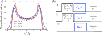
Figure 5: (Color online) (a) Thermally averaged Rabi lineshape fully accounting for trap non-separability. SOC-induced peaks are visible even at $T=3\mu$K. (b) Three pulse sequences used to extract $\theta_{\mathbf{0}q}$ in Fig. (2) of the main text.

Interacting dressed states with a sliding clock superlattice Here, we consider the dynamics of two atoms in neighboring sites $j_{d}(r)$ and $j_{d}(r)+1$ which are tunnel-coupled for a sliding lattice clock phase $\Delta\Upsilon=\pi$. We will take these two atoms to have different transverse mode indices $\mathbf{n}$ and $\mathbf{m}$. Interactions in the $s$-wave channel occur between these atoms when they are in an antisymmetric electronic state $|\Lambda^{-}_{\mathrm{eg}}\rangle\equiv\left(|ge\rangle-|eg\rangle\right)/\sqrt{2}$ with a symmetric spatial wave function $|\Psi^{+}_{\mathbf{nm}}\rangle\equiv\left(|\mathbf{nm}\rangle_{j}+|\mathbf{mn}\rangle_{j}\right)$, with the subscript $j$ denoting the lattice site index. Instead, $p$-wave interactions occur when the atoms are in a symmetric electronic state $|\Lambda^{+}_{\mathrm{eg}}\rangle\equiv\left(|ge\rangle+|eg\rangle\right)/\sqrt{2}$ and an antisymmetric spatial wave function $|\Psi^{-}_{\mathbf{nm}}\rangle\equiv\left(|\mathbf{nm}\rangle_{j}-|\mathbf{mn}\rangle_{j}\right)$. For the purposes of describing the system dynamics at $\Delta\Upsilon=\pi$, where $|\rightarrow\rangle=\left(|g\rangle+|e\rangle\right)/\sqrt{2}$ is the single-well electronic ground state and $|\leftarrow\rangle=\left(|g\rangle-|e\rangle\right)/\sqrt{2}$ the excited state, it is useful to employ the states

$$t,1 :|2^{++},0\rangle,|0,2^{++}\rangle,|\rightarrow_{\mathbf{n}},\rightarrow_{\mathbf{m}}\rangle,|\rightarrow_{\mathbf{m}},\rightarrow_{\mathbf{n}}\rangle\,,$$ (S32)

$$t,-1 :|2^{--},0\rangle,|0,2^{--}\rangle,|\leftarrow_{\mathbf{n}},\leftarrow_{\mathbf{m}}\rangle,|\leftarrow_{\mathbf{m}},\leftarrow_{\mathbf{n}}\rangle$$

$$t,0 :|2^{\pm},0\rangle,|0,2^{\pm}\rangle,\frac{|\rightarrow_{\mathbf{n}},\leftarrow_{\mathbf{m}}\rangle-|\rightarrow_{\mathbf{m}},\leftarrow_{\mathbf{n}}\rangle}{\sqrt{2}},\frac{|\leftarrow_{\mathbf{n}},\rightarrow_{\mathbf{m}}\rangle-|\leftarrow_{\mathbf{m}},\rightarrow_{\mathbf{n}}\rangle}{\sqrt{2}}$$

$$s,0 :|2^{\mp},0\rangle,|0,2^{\mp}\rangle,\frac{|\rightarrow_{\mathbf{n}},\leftarrow_{\mathbf{m}}\rangle+|\rightarrow_{\mathbf{m}},\leftarrow_{\mathbf{n}}\rangle}{\sqrt{2}},\frac{|\leftarrow_{\mathbf{n}},\rightarrow_{\mathbf{m}}\rangle+|\leftarrow_{\mathbf{m}},\rightarrow_{\mathbf{n}}\rangle}{\sqrt{2}}\,,$$

where

$$|2^{++}\rangle =|\rightarrow\rightarrow\rangle|\Psi^{-}_{\mathbf{nm}}\rangle\,,$$ (S33)

$$|2^{--}\rangle =|\leftarrow\leftarrow\rangle|\Psi^{-}_{\mathbf{nm}}\rangle\,,$$ (S34)

$$|2^{\pm}\rangle =\frac{|\rightarrow\leftarrow\rangle+|\leftarrow\rightarrow\rangle}{\sqrt{2}}|\Psi^{-}_{\mathbf{nm}}\rangle\,,$$ (S35)

$$|2^{\mp}\rangle =\frac{|\rightarrow\leftarrow\rangle-|\leftarrow\rightarrow\rangle}{\sqrt{2}}|\Psi^{+}_{\mathbf{nm}}\rangle\,.$$ (S36)

In each four-state sector the Hamiltonian may be written as

$$\hat{H}_{\mu,M_{x}} =2M_{x}\Omega\mathbb{I}+\left(\begin{array}[]{cccc}U_{\mu,M_{x}}&0&J&J\\ 0&U_{\mu,M_{x}}&-J&-J\\ J&-J&0&0\\ J&-J&0&0\end{array}\right)\,,$$ (S41)

where $\mu=t,s$, $U_{t,M_{x}}=V_{M_{x}}$, $U_{s,0}=U_{0}$, $\mathbb{I}$ is the identity operator, and we have set $\Omega_{\mathbf{n}}=\Omega_{\mathbf{m}}=\Omega$ and $J_{\mathbf{n}}=J_{\mathbf{m}}=J$ for simplicity. The $s,0$ singlet sector is rigorously decoupled from the others, but there is mixing between the triplet sectors proportional to the spin model parameters $\chi$ and $C$. These couplings are neglected due to the large single-particle energy difference $\sim\Omega$ between coupled manifolds with the assumed separation of energy scales $\Omega\gg J,V,U$.

The Hamiltonians Eq. (S41) may be readily diagonalized, leading to the eigenvalues $2M_{x}\Omega,2M_{x}\Omega+U,2M_{x}\Omega+\frac{U}{2}\pm\sqrt{4J^{2}+\frac{U^{2}}{4}}$. At high temperatures compared to the tunneling, and for the adiabatic preparation procedure described in the main text, the observed dynamics will be an equal weight superposition of the dynamics from the initial states $|2^{++},0\rangle$, $|0,2^{--}\rangle$, $|\rightarrow_{\mathbf{n}},\leftarrow_{\mathbf{m}}\rangle$, and $|\rightarrow_{\mathbf{m}},\leftarrow_{\mathbf{n}}\rangle$. The dynamics of the number of excitations following adiabatic conversion back to the “bare” $g/e$ basis for these states are

$$|2^{++},0\rangle,|0,2^{--}\rangle\to n_{e}\left(t\right)= 1-\cos\frac{V_{1}t}{2}\cos\left(t\sqrt{4J^{2}+\frac{V_{1}^{2}}{4}}\right)-\frac{V_{1}\sin\frac{V_{1}t}{2}\sin\left(t\sqrt{4J^{2}+V_{1}^{2}/4}\right)}{\sqrt{16J^{2}+V_{1}^{2}}}\,,$$ (S42)

$$|\rightarrow_{\mathbf{n}},\leftarrow_{\mathbf{m}}\rangle,|\rightarrow_{\mathbf{m}},\leftarrow_{\mathbf{n}}\rangle\to n_{e}\left(t\right)= 1-\frac{1}{2}\left(\cos\frac{V_{0}t}{2}\cos\left(t\sqrt{4J^{2}+\frac{V_{0}^{2}}{4}}\right)+\cos\frac{U_{0}t}{2}\cos\left(t\sqrt{4J^{2}+\frac{U_{0}^{2}}{4}}\right)\right)$$ (S43)

$$-\frac{1}{2}\left(\frac{V_{0}\sin\frac{V_{0}t}{2}\sin\left(t\sqrt{4J^{2}+V_{0}^{2}/4}\right)}{\sqrt{16J^{2}+V_{0}^{2}}}+\frac{U_{0}\sin\frac{U_{0}t}{2}\sin\left(t\sqrt{4J^{2}+U_{0}^{2}/4}\right)}{\sqrt{16J^{2}+U_{0}^{2}}}\right)\,.$$

For small interactions compared to tunneling, we can expand the result to lowest order in interactions, and find the thermally averaged dynamics

$$n_{e}\left(t\right) =2\sin^{2}\left(Jt\right)-\frac{\left(U_{0}^{2}+V_{0}^{2}+2V_{1}^{2}\right)t\left(\sin\left(2Jt\right)-2Jt\cos\left(2Jt\right)\right)}{64J}\,.$$ (S44)

In addition to the above two-particle dynamics, there will be contributions from experimental realizations in which the resonant double well has only a single particle. Here, the dynamics is $n_{e}\left(t\right)=\sin^{2}\left(Jt\right)$. Writing $p_{1}$ as the probability of a single particle in a given double well and $p_{2}$ as the probability of having two particles, the small-interaction dynamics averaged over all realizations is hence

$$n_{e}\left(t\right) =\left(p_{1}+2p_{2}\right)\sin^{2}\left(Jt\right)-p_{2}\frac{\left(U_{0}^{2}+V_{0}^{2}+2V_{1}^{2}\right)t\left(\sin\left(2Jt\right)-2Jt\cos\left(2Jt\right)\right)}{64J}\,.$$ (S45)

Noting that $p_{1}+2p_{2}=N$ is the average number, we can subtract the measurements of $n_{e}\left(t\right)/N$ for two different densities with single- and double-occupancy probabilities $(p_{1},p_{2})$ and $(p_{1}^{\prime},p_{2}^{\prime})$ and numbers $N$ and $N^{\prime}$, respectively, to find

$$\Delta[n_{e}\left(t\right)/N] =-\left(\frac{p_{2}}{N}-\frac{p_{2}^{\prime}}{N^{\prime}}\right)\frac{\left(U_{0}^{2}+V_{0}^{2}+2V_{1}^{2}\right)t\left(\sin\left(2Jt\right)-2Jt\cos\left(2Jt\right)\right)}{64J}\,.$$ (S46)

In this way we separate the single-particle contrast decay due to a thermal spread in $J_{\mathbf{n}}$ from the contrast decay due to interactions.

References

• (1) V. Galitski and I. B. Spielman, Spin-orbit coupling in quantum gases, Nature 494, 49–54 (2013).
• (2) N. Cooper, Quantum Hall States of Ultracold Gases , In Many-Body Physics with Ultracold Gases: Lecture Notes of the Les Houches Summer School: Volume 94, 28 June – 23 July 2010, Salomon, C., Shlyapnikov, G. V., and Cugliandolo, L. F., editors. Oxford University Press, Oxford (2013).
• (3) J. Dalibard, F. Gerbier, G. Juzeliūnas, and P. Öhberg, Colloquium: Artificial gauge potentials for neutral atoms, Rev. Mod. Phys. 83, 1523–1543 (2011).
• (4) N. Goldman, G. Juzeliunas, P. Ohberg, and I. B. Spielman, Light-induced gauge fields for ultracold atoms, Rep. Prog. Phys. 77 126401 ( 2014).
• (5) H. Zhai, Degenerate quantum gases with spin -orbit coupling: a review Rep. Prog. Phys. 78, 026001 (2015).
• (6) B. K. Stuhl, H.-I Lu, L. M. Aycock, D. Genkina, and I. B. Spielman, Visualizing edge states with an atomic Bose gas in the quantum Hall regime, arxiv:1502.02496 (2015).
• (7) M. Mancini, G. Pagano, G. Cappellini, L. Livi, M. Rider, J. Catani, C. Sias, P. Zoller, M. Inguscio, M. Dalmonte, and L. Fallani, Observation of chiral edge states with neutral fermions in synthetic Hall ribbons, arXiv:1502.02495 (2015).
• (8) X. Cui, B. Lian, T.L Ho, B. Lev, and H. Zhai, Synthetic gauge field with highly magnetic lanthanide atoms Phys. Rev. A, 88, 011601 (2013).
• (9) Andrew D. Ludlow, Martin M. Boyd, Jun Ye, E. Peik, and P. O. Schmidt, Optical atomic clocks, Rev. Mod. Phys. 87, 637 (2015).
• (10) M. M. Boyd, T. Zelevinsky, A. D. Ludlow, S. M. Foreman, S. Blatt, T. Ido, and J. Ye, Science 314, 1430 (2006).
• (11) B. J. Bloom, et al., Nature 506, 71 (2014).
• (12) T. L. Nicholson, et al., Nat. Commun. 6, 6896 (2015).
• (13) N. Hinkley, et al., Science 341 , 1215 (2013).
• (14) U. Ichiro et al., Cryogenic optical lattice clocks, Nat. Photon., 9, 185-189 (2015).
• (15) M. J. Martin, M. Bishof, M. D. Swallows, X. Zhang, C. Benko, J. von-Stecher, A. V. Gorshkov, A. M. Rey, and Jun Ye, A quantum many-body spin system in an optical lattice clock, Science 341, 632 - 636 (2013).
• (16) N. D. Lemke, J. von Stecher, J. A. Sherman, A. M. Rey, C. W. Oates, and A. D. Ludlow, $p$-Wave cold collisions in an optical lattice clock, Phys. Rev. Lett. 107, 103902 (2011).
• (17) X. Zhang, M. Bishof, S. L. Bromley, C. V. Kraus, M. S. Safronova, P. Zoller, A. M. Rey, and J. Ye, Spectroscopic observation of SU(N)-symmetric interactions in Sr orbital magnetism, Science 345, 1467 (2014).
• (18) A. M. Rey, A.V. Gorshkov, C.V. Kraus, M. J. Martin, M. Bishof, M. D. Swallows, X. Zhang, C. Benko, J. Ye, N.D. Lemke, and A.D. Ludlow, Probing many-body interactions in an optical lattice clock, Annals Phys. 340, 311 - 351 (2014).
• (19) M. Bishof et al., Inelastic Collisions in Optically Trapped Ultracold Metastable Ytterbium, Phys. Rev. A 84, 052716 (2011).
• (20) A. D. Ludlow, N. D. Lemke, J. A. Sherman, C. W. Oates, G. Qu m ner, J. von Stecher, and A. M. Rey, Cold-collision-shift cancellation and inelastic scattering in a Yb optical lattice clock, Phys. Rev. A 84, 052724 (2011).
• (21) R. A. Williams et al. Synthetic Partial Waves in Ultracold Atomic Collisions, Science335, 314-317 (2012).
• (22) Z. Fu et al.Production of Feshbach molecules induced by spin -orbit coupling in Fermi gases, Nature Physics 10, 110 (2014).
• (23) N. R. Cooper and A. M. Rey, Adiabatic Control of Atomic Dressed States for Transport and Sensing, Phys. Rev. A 92, 021401(R) (2015).
• (24) Michael Lohse, Christian Schweizer, Oded Zilberberg, Monika Aidelsburger, and Immanuel Bloch, A Thouless Quantum Pump with Ultracold Bosonic Atoms in an Optical Superlattice, arXiv:1507.02225 (2015).
• (25) Shuta Nakajima, Takafumi Tomita, Shintaro Taie, Tomohiro Ichinose, Hideki Ozawa, Lei Wang, Matthias Troyer, and Yoshiro Takahashi, Topological Thouless Pumping of Ultracold Fermions, arXiv:1507.02223 (2015).
• (26) Hsin-I Lu et al. Geometrical pumping with a Bose-Einstein condensate, arXiv:1508.04480 (2015).
• (27) D. J. Thouless, Quantization of particle transport, Phys. Rev. B 27, 6083 (1983).
• (28) Lei Wang, Matthias Troyer, and Xi Dai, Topological Charge Pumping in a One-Dimensional Optical Lattice, Phys. Rev. Lett. 111, 026802 (2013).
• (29) Feng Mei et al, Topological insulator and particle pumping in a one-dimensional shaken optical lattice, Phys. Rev. A 90, 063638 (2014).
• (30) Ran Wei and Erich J. Mueller, Anomalous charge pumping in a one-dimensional optical superlattice, Phys. Rev. A 92, 013609 (2015).
• (31) F. Scazza, et al. Observation of two-orbital spin-exchange interactions with ultracold SU(N)-symmetric fermions Nature Phys. 10, 779-784 (2014).
• (32) C. Zhang, S. Tewari, R. M. Lutchyn, and S. Das Sarma, $p_{x}+ip_{y}$ Superfluid from $s$-Wave Interactions of Fermionic Cold Atoms, Phys. Rev. Lett. 101, 160401 (2008). ?
• (33) B. Juliá-Díaz, T. Graß, O. Dutta, D.E. Chang, and M. Lewenstein, Engineering $p$-wave interactions in ultracold atoms using nanoplasmonic traps, Nat. Comm. 4, 2046 (2013).
• (34) F. Cappelinni, et al. Direct observation of coherent inter-orbital spin-exchange dynamics Phys. Rev. Lett. 113, 120402 (2014)
• (35) Michael L. Wall, Kaden R. A. Hazzard, and Ana Maria Rey, Effective many-body parameters for atoms in nonseparable Gaussian optical potentials, Phys. Rev. A 92, 013610 (2015).
• (36) A. Celi, P. Massignan, J. Ruseckas, N. Goldman, I.B. Spielman, G. Juzeliunas, and M. Lewenstein, Synthetic gauge fields in synthetic dimensions, Phys. Rev. Lett. 112, 043001 (2014).
• (37) Dario Hügel and Belén Paredes, Chiral Ladders and the Edges of Chern Insulators, Phys. Rev. A 89, 023619 (2014).
• (38) See the Supplementary Material at [xxx] for a derivation of the density shift in Ramsey spectroscopy, the extraction of the chiral Bloch vector angle in Rabi spectroscopy, and the interaction-induced contrast decay with the sliding clock superlattice.
• (39) Y. Hatsugai, Topological aspects of the quantum Hall effect, J. Phys.: Condens. Matter 9, 2507 (1997).
• (40) L. Tarruell, et al.Creating, moving and merging Dirac points with a Fermi gas in a tunable honeycomb lattice, Nature 483, 302 (2012).
• (41) M. Atala, et al., Direct measurement of the Zak phase in topological Bloch bands, Nat. Phys. 9, 795 (2013)
• (42) L. Duca, et al., An Aharonov-Bohm interferometer for determining Bloch band topology, Science 347, 288 (2015)
• (43) M. Cazalilla and A. M. Rey, Ultracold Fermi Gases with Emergent SU(N) Symmetry, Rep. Prog. Phys. 77, 124401 (2014).