Higgs boson production in association with $b$ jets in the POWHEG BOX

Abstract

The hadronic production of a Higgs boson ($H$) in association with $b$ jets will play an important role in investigating the Higgs-boson couplings to Standard Model particles during Run II of the CERN Large Hadron Collider, and could in particular reveal the presence of anomalies in the assumed hierarchy of Yukawa couplings to the third-generation quarks. A very high degree of accuracy in the theoretical description of this process is crucial to implement the rich physics program that could lead to either direct or indirect evidence of new physics from Higgs-boson measurements. Aiming for accuracy in the theoretical modeling of $H+b$-jet production, we have interfaced the analytic Next-to-Leading-Order QCD calculation of $Hb\bar{b}$ production with parton-shower Monte Carlo event generators in the POWHEG BOX framework. In this paper we describe the most relevant aspects of the implementation and present results for the production of $H+1b$ jet, $H+2b$ jets, and $H$ with no tagged $b$ jets, in the form of kinematic distributions of the Higgs boson, of the $b$ jets, and of the non-$b$ jets, at the 13 TeV Large Hadron Collider. The corresponding code is part of the public release of the POWHEG BOX.

I Introduction

The production of a Higgs boson with $b$ jets at the CERN Large Hadron Collider (LHC) can provide essential information on the Higgs-boson couplings to third generation quarks, in particular to the bottom quark. Indeed, all the leading parton-level production processes ($gg\rightarrow Hb\bar{b}$, $q\bar{q}\rightarrow Hb\bar{b}$, and $bg\rightarrow Hb$) involve a Higgs boson radiated from an external bottom quark, while at the loop-level the Higgs boson can also originate from internal loops of both bottom (leading) and top quarks (see, e.g., the discussion in Dawson et al. (2006); Wiesemann et al. (2015)). In the Standard Model, the Higgs-boson couplings to both fermions and gauge bosons are just proportional to the particles’ masses, causing the Higgs-boson associated production with bottom quarks to be largely suppressed with respect to the major production mechanisms, like gluon-gluon fusion (mediated by a loop of top quarks) or vector-boson fusion and associated production with vector bosons (where the Higgs boson couples to $W$ or $Z$ bosons). The production with $b$ jets is then further suppressed by the identification cuts usually placed on $b$ jets for tagging purposes. This scenario can however be drastically different if the hierarchy of Higgs-boson Yukawa couplings is modified by factors that typically enter in models with extended Higgs sectors, like Two Higgs Doublet Models. In the quest for unveiling the origin of the breaking of the electroweak gauge symmetry, the evidence for (or absence of) $H+b$-jet production at Run II of the LHC can therefore provide an essential piece of the puzzle.

In view of its crucial role for the Higgs-boson physics program of Run II of the LHC, $H+b$-jets production has received quite some attention in the context of the LHC Higgs Cross Section Working Group Dittmaier et al. (2011, 2012); Heinemeyer et al. (2013), and both ATLAS and CMS have used the $Hb\bar{b}$ production channel in all major studies to constrain supersymmetric models and other extensions of the Standard Model Chatrchyan et al. (2013); Khachatryan et al. (2014, 2015a); Khachatryan et al. (2015b); Aad et al. (2014). On the theoretical side, it is essential to control and improve the accuracy with which we can estimate rates for $H$ production with one or two $b$ jets, and, with this regard, quite some progress has been made in the last few years. In the following we will briefly summarize the main results obtained in this context, while we refer to the existing literature for more exhaustive explanations and details.

As for all processes involving multiple scales (such as the masses of the bottom quark or the Higgs boson, $m_{b}$ and $M_{H}$, as well as scales determined by the kinematics of collisions at TeV center-of-mass energies), the QCD perturbative prediction of $H+b$-quark production can be affected by the presence, at all orders, of large corrections proportional to logarithms of ratios of these mass scales (e. g., $\log(m_{b}/Q)$ where indicatively one can assume $Q\sim M_{H}$ or larger). The occurrence of these enhanced logarithmic corrections depends on the signature studied as well as on the kinematic regime considered. It can be shown that these corrections can be reabsorbed in the perturbative definition of a bottom-quark parton distribution function, and from this observation originates the prescription to calculate processes like $H+b$ quarks in a 5 Flavor Scheme (5FS) where the $b$ quark is treated as a light parton and can appear in the initial state. At fixed perturbative order this is an alternative to the usual 4 Flavor Scheme (4FS) calculation where only four light-flavor parton densities are assumed while the bottom quark is treated as massive and can only appear in the final state. The production of $H+1b$ jet can be induced at tree level by $bg\rightarrow bH$ in the 5FS, and by $q\bar{q},gg\rightarrow Hb\bar{b}$ in the 4FS; while the production of $H+2b$ jets can only arise at lowest order via $q\bar{q},gg\rightarrow Hb\bar{b}$ and is therefore an unambiguous 4FS prediction. The two approaches only correspond to a different reordering of the (same) perturbative expansion, and their predictions tend to agree better the higher the perturbative order, showing the expected well behaved convergence of QCD predictions. Several discussions of this issue can be found in the literature, where the general 4FS/5FS formalism is thoroughly analyzed Maltoni et al. (2012); Febres Cordero and Reina (2015) as well as specialized to the particular case of $H+b$-quark production Campbell et al. (2004); Dawson et al. (2006); Heinemeyer et al. (2013); Wiesemann et al. (2015).

Next-to-Leading Order (NLO) QCD corrections to $H+b$ jet production have been calculated both in the 5FS Campbell et al. (2003) and in the 4FS Dittmaier et al. (2004); Dawson et al. (2004, 2005). The first set of corrections is nowadays part of the NLO QCD 5FS prediction of $H+1b$ jet Campbell et al. (2003); Campbell and Ellis (2011); Heinemeyer et al. (2013), while the second set of corrections are included in the NLO QCD 4FS prediction of both $H+1b$ jet Dawson et al. (2005) and $H+2b$ jets  Dittmaier et al. (2004); Dawson et al. (2004); Heinemeyer et al. (2013). NLO QCD fixed-order results for both $Hb$ and $Hb\bar{b}$ hadronic production can also be obtained via any of the public NLO automated tools such as MadGraph5_aMC@NLO Alwall et al. (2014), GoSam Cullen et al. (2014), or OpenLoops Cascioli et al. (2012). Of course, the totally inclusive cross section (with no $b$ tagging) can be calculated in either scheme, and dedicated studies which includes up to Next-to-Next-to-Leading-Order (NNLO) QCD corrections have been presented in the literature Dicus et al. (1999); Maltoni et al. (2003); Harlander and Kilgore (2003); Campbell et al. (2004); Dawson et al. (2006); Heinemeyer et al. (2013); Wiesemann et al. (2015).

In order to improve the accuracy of theoretical predictions for total cross sections and distributions, these NLO fixed-order results need to be consistently interfaced with parton-shower Monte Carlo generators like PYTHIA Sjostrand et al. (2006, 2008) and HERWIG Marchesini et al. (1992); Corcella et al. (2001) using one of the methods proposed in the literature, namely MC@NLO Frixione and Webber (2002); Frixione et al. (2003) and POWHEG Nason (2004); Frixione et al. (2007a, b), as implemented in specific frameworks like, e. g., MadGraph5_aMC@NLO Hirschi et al. (2011); Alwall et al. (2014), the POWHEG BOX Alioli et al. (2010), and SHERPA Gleisberg et al. (2009). The implementation of Higgs-boson production with $b$ quarks in MadGraph5_aMC@NLO has been discussed in Ref. Wiesemann et al. (2015), where total cross sections have been given for both inclusive and exclusive production and distributions have been shown in particular for the inclusive case (no $b$-jet tagging). In this paper we present the implementation of $H+b$-jet production in the POWHEG BOX, based on the 4FS NLO QCD calculation of $Hb\bar{b}$ hadronic production of Ref. Dawson et al. (2004). While Ref. Wiesemann et al. (2015) considers both the 5FS and a 4FS cases, we will only consider the 4FS case since we aim at presenting in particular results for both $H+1b$ jet and $H+2b$ jets in the same framework. We note that the implementation of $b$-initiated processes in a NLO QCD parton-shower Monte Carlo is still being studied and, to our knowledge, it is not routinely available in any of the aforementioned frameworks. Hence our decision to only implement the 4FS case. The details of the implementation will be presented in Section II. Results for $H+1b$-jet, $H+2b$-jet, and $H$ with no tagged $b$ jet will be given in Section III, using a specific setup, for the purpose of illustrating the kind of studies that are now possible within the POWHEG BOX framework. Our conclusion are presented in Section IV.

II Implementation

The implementation of the $Hb\bar{b}$ process in the framework of the POWHEG BOX can be performed along the same lines as the related $Ht\bar{t}$ process that has been considered in Ref. Hartanto et al. (2015). While the POWHEG BOX package provides all process-independent building blocks, it requires a list of all independent flavor structures for the tree-level contributions at Leading Order (LO) and NLO, the Born and real-emission amplitudes squared, the finite parts of the virtual contributions, the color- and spin-correlated amplitudes squared, and a parametrization of the phase space for the Born process. The flavor structures and tree-level amplitudes can most conveniently be generated with the help of a tool based on MadGraph 4 Stelzer and Long (1994); Alwall et al. (2007) that is provided in the POWHEG BOX. The virtual contributions for the $pp\to Hb\bar{b}$ process are extracted from the NLO-QCD calculation of Dawson et al. (2004) and adapted to the format required by the POWHEG BOX. All building blocks are implemented in the 4FS, i.e. no contributions from incoming bottom quarks are taken into account and the bottom-quark mass is always considered to be non-zero.

While at LO and in the real-emission contributions only diagrams including a $Hb\bar{b}$ coupling emerge, in the virtual corrections also loop diagrams with a $Ht\bar{t}$ coupling contribute. These are fully taken into account in the representative results discussed in this work. The user of the POWHEG BOX implementation can choose to de-activate the contributions including a top-quark Yukawa coupling via a switch in the input file. This allows to rescale separately the two contributions as necessary to calculate $Hb\bar{b}$ production in, for instance, supersymmetric extensions of the Standard Model, as discussed in detail in Dawson et al. (2006), where also a rescaling prescription is provided.

We note that, contrary to the case of $Ht\bar{t}$ production, where the heavy-quark mass is typically renormalized in the on-shell renormalization scheme, in the case of $Hb\bar{b}$ production the renormalized bottom-quark mass is often defined in the $\overline{\mathrm{MS}}$ renormalization scheme Dawson et al. (2004, 2006). While both renormalization schemes are perturbatively equivalent at NLO with differences only due to higher-order contributions, $Hb\bar{b}$ production processes have been found to be quite sensitive to the renormalization scheme via the bottom-mass dependence of the overall bottom-quark Yukawa coupling. Indeed, as higher-order corrections beyond the one-loop level are partly taken care of, physical observables are often found to exhibit a better perturbative behavior when the $\overline{\mathrm{MS}}$ scheme is used for the the bottom-quark Yukawa coupling. Taking this into account, the results presented below have been obtained in the $\overline{\mathrm{MS}}$ scheme. When using the POWHEG BOX implementation of the $Hb\bar{b}$ process, however, the user is free to choose either the on-shell or the $\overline{\mathrm{MS}}$ renormalization scheme for the bottom-quark mass that enters the Yukawa coupling by setting the respective parameter in the input file.

Although in principle not necessary for obtaining finite results, technical cuts at the generation level can help to improve the performance of the Monte-Carlo integration. For the computation of observables with identified $b$ jets we therefore recommend the use of a small cut on the transverse-momentum of the bottom quarks (e.g. $p_{T}^{\mathrm{cut}}=0.1$ GeV) when the phase-space integration is performed. We have checked that final results for the respective scenarios in Section III do not change when generation cuts of $p_{T}^{\mathrm{cut}}=0.1$ GeV or $p_{T}^{\mathrm{cut}}=1$ GeV are imposed compared to the case where no generation cuts are applied.

In order to verify the POWHEG BOX implementation of the $Hb\bar{b}$ process, we have performed a detailed comparison of cross sections and distributions at LO and NLO as obtained in the POWHEG BOX with the fixed-order code of Dawson et al. (2004), and found full agreement for all considered observables. In addition we have successfully compared our results to those of Ref. Wiesemann et al. (2015).

III Results

The code we developed is available from the webpage of the POWHEG BOX project, http://powhegbox.mib.infn.it/. With this version of the code the user is free to study $Hb\bar{b}$ production at a hadron collider in a customized setup. Here, we wish to discuss representative results for $Hb\bar{b}$ production at the LHC with a center-of-mass energy of $\sqrt{s}=13$ TeV. We use the four-flavor MSTW2008 set of parton distribution functions Martin et al. (2009, 2010) as implemented in the LHAPDF library Whalley et al. (2005), with the associated value of $\alpha_{s}$, a Higgs-boson mass of $m_{H}=125$ GeV, and a top-quark mass of $m_{t}=173$ GeV. The on-shell mass of the bottom quark is set to $m_{b}^{\mathrm{OS}}=4.75$ GeV, resulting in an $\overline{\mathrm{MS}}$ mass of $\overline{m}_{b}(\overline{m}_{b})=4.34$ GeV at NLO QCD.

For the renormalization ($\mu_{\mathrm{R}}$) and factorization ($\mu_{\mathrm{F}}$) scales we consider two options: first we use a fixed scale,

$$\mu_{0}=\frac{m_{H}+2m_{b}}{4}\,,$$ (1)

and second a dynamical scale,

$$\mu_{0}=\frac{1}{4}\sum_{i}\sqrt{m_{i}^{2}+p_{T,i}^{2}}\,,$$ (2)

where the summation runs over the masses and transverse momenta of the Higgs boson and the partons in the final state of the fixed-order calculation. To assess the scale dependence of our predictions, we vary the renormalization and factorization scales, $\mu_{\mathrm{R}}=\xi\mu_{0}$ and $\mu_{\mathrm{F}}=\xi\mu_{0}$ simultaneously in the range $\xi=1/2$ to $\xi=2$.

We have matched the fixed-order NLO calculation with PYTHIA-6.4.25. In order to be able to focus our discussion of the NLO+PYTHIA results on genuine parton-shower effects, we did not activate multi-parton interactions, underlying event effects, or decays of the Higgs boson in the Monte-Carlo program, although each of these effects could in principle be accounted for by setting the respective parameters in PYTHIA.

In our numerical analysis we consider the two scenarios with a Higgs boson produced in association with one or two identified $b$ jets, as well as the case with no tagged $b$ jets. Jets of any type are reconstructed with the anti-$k_{T}$ algorithm as implemented in the FASTJET package Cacciari et al. (2012), with $R=0.5$. A jet that contains either a bottom quark or antiquark, or a $B$ meson, is considered a $b$ jet. For our $H+2b$-jet analysis, we require at least two $b$ jets with a minimum transverse momentum in the central region of pseudorapidity,

$$p_{T}(b\!-\!\mathrm{jet})>25~{}\mathrm{GeV}\,,\quad|\,\eta(b\!-\!\mathrm{jet})|<2.5\,,$$ (3)

while for the $H+1b$-jet analysis only one identified $b$ jet fulfilling the above criteria is required. We do not impose any cuts on extra jets, unless stated otherwise.

In Figs. 1-2 we illustrate the impact of the parton shower on the fixed-order NLO QCD results for the transverse-momentum ($p_{T}$) and pseudorapidity ($\eta$) distributions of the Higgs boson and the hardest of the identified $b$ jets in $H+2b$-jet production, respectively, for both the fixed- and the dynamical-scale choice $\mu_{\mathrm{F}}=\mu_{\mathrm{R}}=\mu_{0}$ of Eqs. (1) and (2), respectively. In Figs. 3-4 we show the corresponding distributions for $H+1b$-jet production, and in Fig. 5 we show the $p_{T}(H)$ and $\eta(H)$ distributions for the inclusive case, i.e. when no $b$ jets are tagged. We find that parton-shower effects do not significantly change the fixed-order NLO results of these distributions within the given statistical uncertainty in most of the kinematic regimes shown. Only in the Higgs $p_{T}$ distributions for all signatures, $H+0,1,2b$ jets, we find that parton-shower effects decrease (enhance) the NLO results for small (large) values of $p_{T}(H)$. These distributions also show that the effects of the parton shower do not significantly differ for a fixed- and dynamical-scale choice within their respective statistical uncertainties.

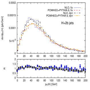
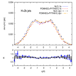
Figure 1: The $p_{T}$ (left) and $\eta$ (right) distributions of the Higgs boson in $H+2b$-jet production at NLO-QCD with no parton shower (blue short-dashed line for fixed scale, black long-dash-dotted line for dynamical scale), and with parton shower as obtained through POWHEG+PYTHIA6 (red medium-dashed line for fixed scale, orange long-dash-dotted line for dynamical scale). The lower panels show the ratios: $R=d\sigma(\mathrm{NLO})/d\sigma({\tt POWHEG\!+\!PYTHIA}{})$ for a fixed (blue points) and a dynamical (black points) scale, respectively. The error bars indicate the statistical uncertainties of the Monte-Carlo integration.

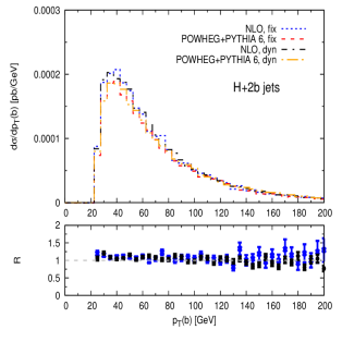
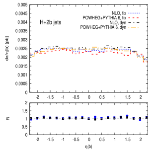
Figure 2: The $p_{T}$ (left) and $\eta$ (right) distributions of the hardest identified $b$ jet in $H+2b$-jet production at NLO-QCD with no parton shower (blue short-dashed line for fixed scale, black long-dash-dotted line for dynamical scale), and with parton shower as obtained through POWHEG+PYTHIA6 (red medium-dashed line for fixed scale, orange long-dash-dotted line for dynamical scale). The lower panels show the ratios: $R=d\sigma(\mathrm{NLO})/d\sigma({\tt POWHEG\!+\!PYTHIA}{})$ for a fixed (blue points) and a dynamical (black points) scale, respectively. The error bars indicate the statistical uncertainties of the Monte-Carlo integration.

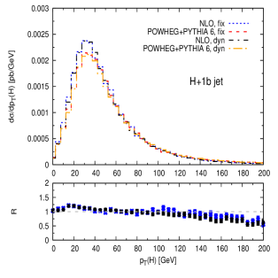
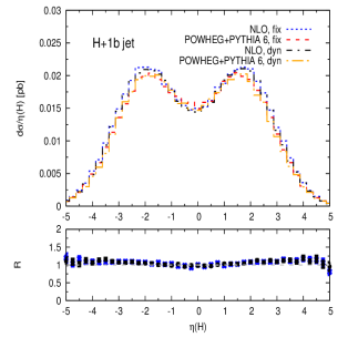
Figure 3: The $p_{T}$ (left) and $\eta$ (right) distributions of the Higgs boson in $H+1b$-jet production at NLO-QCD with no parton shower (blue short-dashed line for fixed scale, black long-dash-dotted line for dynamical scale), and with parton shower as obtained through POWHEG+PYTHIA6 (red medium-dashed line for fixed scale, orange long-dash-dotted line for dynamical scale). The lower panels show the ratios: $R=d\sigma(\mathrm{NLO})/d\sigma({\tt POWHEG\!+\!PYTHIA}{})$ for a fixed (blue points) and a dynamical (black points) scale, respectively. The error bars indicate the statistical uncertainties of the Monte-Carlo integration.

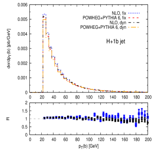
Figure 4: The $p_{T}$ (left) and $\eta$ (right) distributions of the hardest identified $b$ jet in $H+1b$-jet production at NLO-QCD with no parton shower (blue short-dashed line for fixed scale, black long-dash-dotted line for dynamical scale), and with parton shower as obtained through POWHEG+PYTHIA6 (red medium-dashed line for fixed scale, orange long-dash-dotted line for dynamical scale). The lower panels show the ratios: $R=d\sigma(\mathrm{NLO})/d\sigma({\tt POWHEG\!+\!PYTHIA}{})$ for a fixed (blue points) and a dynamical (black points) scale, respectively. The error bars indicate the statistical uncertainties of the Monte-Carlo integration.

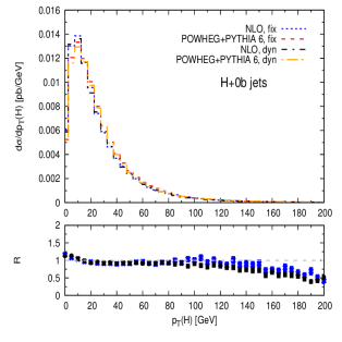
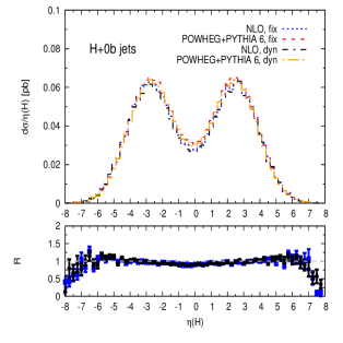
Figure 5: The $p_{T}$ (left) and $\eta$ (right) distributions of the Higgs boson in the inclusive case at NLO-QCD with no parton shower (blue short-dashed line for fixed scale, black long-dash-dotted line for dynamical scale), and with parton shower as obtained through POWHEG+PYTHIA6 (red medium-dashed line for fixed scale, orange long-dash-dotted line for dynamical scale). The lower panels show the ratios: $R=d\sigma(\mathrm{NLO})/d\sigma({\tt POWHEG\!+\!PYTHIA}{})$ for a fixed (blue points) and a dynamical (black points) scale, respectively. The error bars indicate the statistical uncertainties of the Monte-Carlo integration.

In Fig. 6 (left), we show the effect of the parton shower on correlations of the two identified $b$ jets in the $H+2b$-jet case, in particular their invariant mass distribution ($M(bb)$) and their separation in the azimuthal-angle-pseudorapidity plane ($R(b,b)$). The impact of the parton shower is again not significant within the statistical errors (apart for very small values of $M(bb)$).

To illustrate the behavior of distributions including a non-$b$ jet we show in Fig. 7 the $R(b,j)$ distribution in the $H+2b$-jet case, where $R(b,j)$ is the separation of the hardest $b$ jet and the hardest non-$b$ jet in the azimuthal-angle-pseudorapidity plane. Here, we only consider non-$b$ jets with a transverse momentum larger than 25 GeV in the rapidity region of the detector $|y_{j}|<4.5$. In the l.h.s. plot we show the comparison between fixed-order NLO results and results obtained after the same calculation is interfaced with PYTHIA6 in the POWHEG BOX framework, for the central value of both the fixed and dynamical scale. Since the effect of parton shower and in particular of scale dependence (fixed vs dynamical) seems much bigger than for other distributions, we further investigate the scale dependence of the distribution, which is shown in the r.h.s plot of Fig. 7. Clearly, the $R(b,j)$ distribution is affected by a large scale uncertainty, both for a fixed- and a dynamical-scale choice. This is typical of observables that are indeed effectively described only at LO by a given NLO calculation. In the case of $Hb\bar{b}$ production, the hardest non-$b$ jet can only stem from the real-emission contributions of the hard matrix element (namely $q\bar{q},gg\rightarrow Hb\bar{b}+g$ or $qg,\bar{q}g\rightarrow Hb\bar{b}+q/\bar{q}$), or from extra radiation due to the parton shower. Therefore, distributions of the hardest non-$b$ jet are effectively described only with LO accuracy and are affected by a typical LO scale uncertainty. Gaining full NLO control on jet distributions with smaller scale uncertainties would require an NLO calculation for $pp\to Hb\bar{b}+\mathrm{jet}$. The different behavior for fixed- and dynamical-scale choices which appears in the l.h.s. plot of Fig. 7 (where only the central value of each scale is used) is then due to the large scale uncertainty encountered in distributions effectively only described to LO accuracy in the fixed-order calculation. We find large differences between the fixed-order predictions with $\xi=2$ and $\xi=0.5$ when choosing $\mu_{\mathrm{R}}=\mu_{\mathrm{F}}=\xi\mu_{0}$ with $\mu_{0}$ defined in Eqs. (1) and (2). These differences are reduced once the fixed-order calculation is combined with the parton shower in the POWHEG+PYTHIA6 predictions.

Indeed, to illustrate the effect of the parton shower on non-$b$-jet observables we show in Fig. 8 the transverse momentum of the hardest non-$b$ jet, but this time with no cut applied on the non-$b$ jet. If no $p_{T}$ cuts are imposed on the non-$b$ jets, in a fixed-order calculation the transverse-momentum distribution of a non-$b$ jet becomes very large at small values of $p_{T}$, which is due to large contributions from the emission of partons of very soft or collinear type. This behavior is tamed once the POWHEG-Sudakov factor is applied, as it is the case in the POWHEG+PYTHIA result shown in Fig. 8 for the case of inclusive and $H+2b$-jet production. Since this effect is not sensitive to the tagging of $b$ jets, similar shapes are encountered in both analysis scenarios (and also in the $H+1b$-jet scenario which is not explicitly shown here).

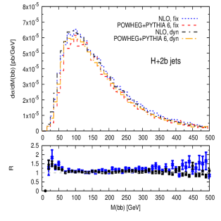
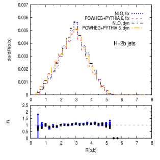
Figure 6: The $M(bb)$ (left) and $R(b,b)$ (right) distributions in $H+2b$-jet production at NLO-QCD with no parton shower (blue short-dashed line for fixed scale, black long-dash-dotted line for dynamical scale), and with parton shower as obtained through POWHEG+PYTHIA6 (red medium-dashed line for fixed scale, orange long-dash-dotted line for dynamical scale). The lower panels show the ratios: $R=d\sigma(\mathrm{NLO})/d\sigma({\tt POWHEG\!+\!PYTHIA}{})$ for a fixed (blue points) and a dynamical (black points) scale, respectively. The error bars indicate the statistical uncertainties of the Monte-Carlo integration.

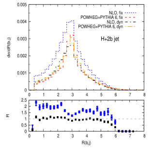
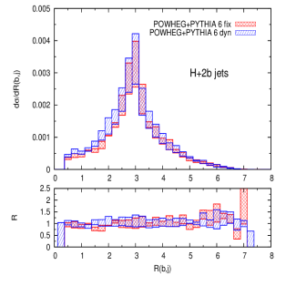
Figure 7: The $R(b,j)$ distribution in $H+2b$-jet production. The l.h.s. plot shows a comparison of NLO-QCD with no parton shower (blue short-dashed line for fixed scale, black long-dash-dotted line for dynamical scale), and with parton shower as obtained through POWHEG+PYTHIA6 (red medium-dashed line for fixed scale, orange long-dash-dotted line for dynamical scale). The lower panel shows the ratios: $R=d\sigma(\mathrm{NLO})/d\sigma({\tt POWHEG\!+\!PYTHIA}{})$ for a fixed (blue points) and a dynamical (black points) scale, respectively. The r.h.s. plot shows the $R(b,j)$ NLO QCD distribution as obtained with POWHEG+PYTHIA6 for different values of the fixed ($fix$) and dynamical ($dyn$) renormalization/factorization scales, $\mu=\xi\mu_{0}$ with $\xi=(0.5;2)$. The lower panel shows the respective ratios $R=d\sigma(\xi\mu_{0})/d\sigma(\mu_{0})$. The error bars in the lower panels of both l.h.s. and r.h.s. plots indicate the statistical uncertainties of the Monte-Carlo integration.

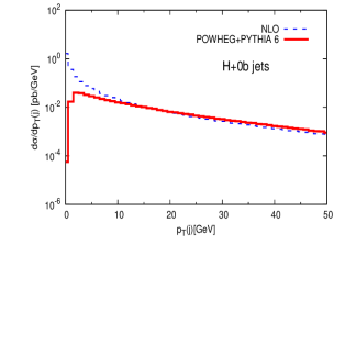
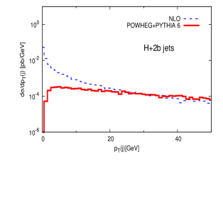
Figure 8: Transverse-momentum distribution of the hardest non-$b$ jet for the case of inclusive (left) and $H+2b$-jet production (right) at NLO-QCD with no parton shower (dashed, blue), and with parton shower as obtained through POWHEG+PYTHIA6 (solid, red), for a dynamical scale choice.

In order to assess the theoretical uncertainties associated with the choice of renormalization and factorization scale for NLO distributions, we have computed the $p_{T}$ and $\eta$ distributions of the Higgs boson for all three signatures, i.e. $H+0,1,2b$ jets, and the $p_{T}$ and $\eta$ distributions of the hardest identified $b$ jet for both $H+1b$-jet and $H+2b$-jet production, for different choices of scales as discussed earlier. The corresponding results, obtained using our POWHEG+PYTHIA6 implementation, are shown in Fig. 9 (no $b$ tagging), Figs. 10-11 ($H+1b$ jet), and Figs. 12-13 ($H+2b$ jets). The scale dependence of the results is considerable, amounting to about $\pm 25\%$ in most regions of phase space. Using a fixed scale rather than a dynamical scale helps in slightly reducing the scale uncertainty of the NLO+PYTHIA results in all observables, especially at larger values of $p_{T}(b)$, $p_{T}(H)$ and in the central pseudorapidity region, although the effect is moderate. We note that also the total cross sections in the three scenarios considered here exhibit a large scale uncertainty, for instance we find $\sigma=0.477\,{\rm pb}\pm 18\%$ for the total inclusive cross section obtained with our NLO+PYTHIA6 implementation in the setup of Fig. 9 for a fixed-scale choice.

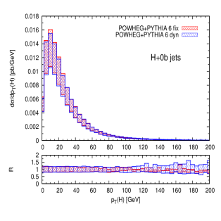
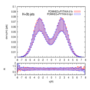
Figure 9: The $p_{T}$ (left) and $\eta$ (right) distributions of the Higgs boson in the inclusive-production case as obtained with POWHEG+PYTHIA6 for different values of the fixed ($fix$) and dynamical ($dyn$) renormalization/factorization scales, $\mu=\xi\mu_{0}$ with $\xi=(0.5;2)$. The lower panels show the respective ratios $R=d\sigma(\xi\mu_{0})/d\sigma(\mu_{0})$.

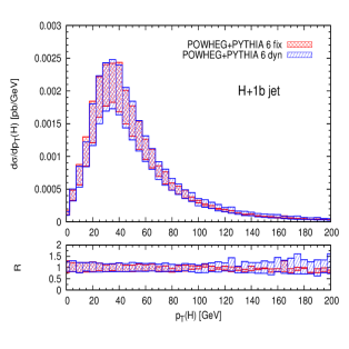
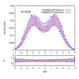
Figure 10: The $p_{T}$ (left) and $\eta$ (right) distributions of the Higgs boson in $H+1b$-jet production as obtained with POWHEG+PYTHIA6 for different values of the fixed ($fix$) and dynamical ($dyn$) renormalization/factorization scales, $\mu=\xi\mu_{0}$ with $\xi=(0.5;2)$. The lower panels show the respective ratios $R=d\sigma(\xi\mu_{0})/d\sigma(\mu_{0})$.

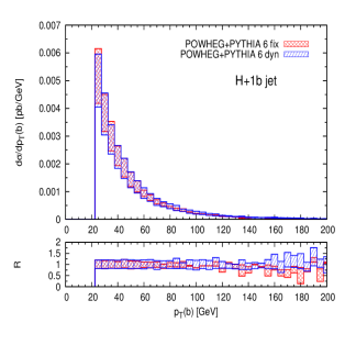
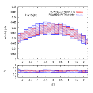
Figure 11: The $p_{T}$ (left) and $\eta$ (right) distributions of the hardest identified $b$ jet in $H+1b$-jet production as obtained with POWHEG+PYTHIA6 for different values of the fixed ($fix$) and dynamical ($dyn$) renormalization/factorization scales, $\mu=\xi\mu_{0}$ with $\xi=(0.5;2)$. The lower panels show the respective ratios $R=d\sigma(\xi\mu_{0})/d\sigma(\mu_{0})$.

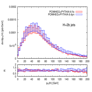
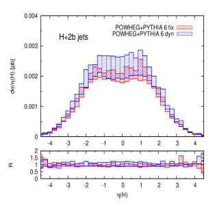
Figure 12: The $p_{T}$ (left) and $\eta$ (right) distributions of the Higgs boson in $H+2b$-jet production as obtained with POWHEG+PYTHIA6 for different values of the fixed ($fix$) and dynamical ($dyn$) renormalization/factorization scales, $\mu=\xi\mu_{0}$ with $\xi=(0.5;2)$. The lower panels show the respective ratios $R=d\sigma(\xi\mu_{0})/d\sigma(\mu_{0})$.

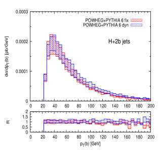
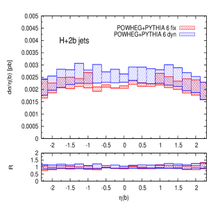
Figure 13: The $p_{T}$ (left) and $\eta$ (right) distributions of the hardest identified $b$ jet in $H+2b$-jet production as obtained with POWHEG+PYTHIA6 for different values of the fixed ($fix$) and dynamical ($dyn$) renormalization/factorization scales, $\mu=\xi\mu_{0}$ with $\xi=(0.5;2)$. The lower panels show the respective ratios $R=d\sigma(\xi\mu_{0})/d\sigma(\mu_{0})$.

IV Conclusions

In this article we have presented the implementation of the NLO QCD calculation for $Hb\bar{b}$ production at a hadron collider (from Ref. Dawson et al. (2004)) in the POWHEG BOX package. We emphasize how having $H+b$-jet production available in the POWHEG BOX provides a crucial element of consistency for experimental studies that rely on the same framework for a broad variety of signal and background processes. The code is made publicly available so that it can be used for further studies of $Hb\bar{b}$ production at the LHC in the SM and in extensions of the SM with modified Yukawa couplings of the third generation quarks. Here, we considered the SM and presented numerical results at fixed perturbative order and at NLO QCD matched with PYTHIA for selected representative setups. In particular, we discussed theoretical uncertainties due to factorization/renormalization scale choices and variations and parton-shower effects for two analysis scenarios with a Higgs boson in association with one or two $b$ jets, respectively. A sample of results for the case of inclusive production have also been presented. We found that parton-shower effects do not give rise to large distortions of observables related to the Higgs boson or identified $b$ jets in $H+1b$-jet and $H+2b$-jet production processes at the LHC. As expected, more pronounced effects occur in distributions involving non-$b$ jets, as shown, for example, by the transverse-momentum distribution of the hardest non-$b$ jet or by the distribution of the separation ($R(b,j)$) between the hardest $b$ jet and the hardest non-$b$ jet. We studied the impact of different scale choices on various distributions and found that the associated theoretical uncertainties can be considerable.

References

- Dawson et al. (2006) S. Dawson, C. B. Jackson, L. Reina, and D. Wackeroth, Mod. Phys. Lett. A21, 89 (2006), eprint hep-ph/0508293.
- Wiesemann et al. (2015) M. Wiesemann, R. Frederix, S. Frixione, V. Hirschi, F. Maltoni, and P. Torrielli, JHEP 02, 132 (2015), eprint 1409.5301.
- Dittmaier et al. (2011) S. Dittmaier et al. (LHC Higgs Cross Section Working Group) (2011), eprint 1101.0593.
- Dittmaier et al. (2012) S. Dittmaier, S. Dittmaier, C. Mariotti, G. Passarino, R. Tanaka, et al. (2012), eprint 1201.3084.
- Heinemeyer et al. (2013) S. Heinemeyer et al. (LHC Higgs Cross Section Working Group) (2013), eprint 1307.1347.
- Chatrchyan et al. (2013) S. Chatrchyan et al. (CMS), Phys. Lett. B722, 207 (2013), eprint 1302.2892.
- Khachatryan et al. (2014) V. Khachatryan et al. (CMS), JHEP 10, 160 (2014), eprint 1408.3316.
- Khachatryan et al. (2015a) V. Khachatryan et al. (CMS) (2015a), eprint 1508.01437.
- Khachatryan et al. (2015b) V. Khachatryan et al. (CMS) (2015b), eprint 1506.08329.
- Aad et al. (2014) G. Aad et al. (ATLAS), JHEP 11, 056 (2014), eprint 1409.6064.
- Maltoni et al. (2012) F. Maltoni, G. Ridolfi, and M. Ubiali, JHEP 07, 022 (2012), [Erratum: JHEP04,095(2013)], eprint 1203.6393.
- Febres Cordero and Reina (2015) F. Febres Cordero and L. Reina, Int. J. Mod. Phys. A30, 1530042 (2015), eprint 1504.07177.
- Campbell et al. (2004) J. M. Campbell, S. Dawson, S. Dittmaier, C. Jackson, M. Kramer, F. Maltoni, L. Reina, M. Spira, D. Wackeroth, and S. Willenbrock, in Physics at TeV colliders. Proceedings, Workshop, Les Houches, France, May 26-June 3, 2003 (2004), eprint hep-ph/0405302.
- Campbell et al. (2003) J. M. Campbell, R. K. Ellis, F. Maltoni, and S. Willenbrock, Phys. Rev. D67, 095002 (2003), eprint hep-ph/0204093.
- Dittmaier et al. (2004) S. Dittmaier, M. Kramer, 1, and M. Spira, Phys. Rev. D70, 074010 (2004), eprint hep-ph/0309204.
- Dawson et al. (2004) S. Dawson, C. B. Jackson, L. Reina, and D. Wackeroth, Phys. Rev. D69, 074027 (2004), eprint hep-ph/0311067.
- Dawson et al. (2005) S. Dawson, C. B. Jackson, L. Reina, and D. Wackeroth, Phys. Rev. Lett. 94, 031802 (2005), eprint hep-ph/0408077.
- Campbell and Ellis (2011) J. M. Campbell and R. K. Ellis, Mcfm, from v.6 (2011), http://mcfm.fnal.gov.
- Alwall et al. (2014) J. Alwall, R. Frederix, S. Frixione, V. Hirschi, F. Maltoni, et al., JHEP 1407, 079 (2014), eprint 1405.0301.
- Cullen et al. (2014) G. Cullen, H. van Deurzen, N. Greiner, G. Heinrich, G. Luisoni, et al., Eur.Phys.J. C74, 3001 (2014), eprint 1404.7096.
- Cascioli et al. (2012) F. Cascioli, P. Maierhofer, and S. Pozzorini, Phys.Rev.Lett. 108, 111601 (2012), eprint 1111.5206.
- Dicus et al. (1999) D. Dicus, T. Stelzer, Z. Sullivan, and S. Willenbrock, Phys. Rev. D59, 094016 (1999), eprint hep-ph/9811492.
- Maltoni et al. (2003) F. Maltoni, Z. Sullivan, and S. Willenbrock, Phys. Rev. D67, 093005 (2003), eprint hep-ph/0301033.
- Harlander and Kilgore (2003) R. V. Harlander and W. B. Kilgore, Phys. Rev. D68, 013001 (2003), eprint hep-ph/0304035.
- Sjostrand et al. (2006) T. Sjostrand, S. Mrenna, and P. Z. Skands, JHEP 0605, 026 (2006), eprint hep-ph/0603175.
- Sjostrand et al. (2008) T. Sjostrand, S. Mrenna, and P. Z. Skands, Comput.Phys.Commun. 178, 852 (2008), eprint 0710.3820.
- Marchesini et al. (1992) G. Marchesini, B. Webber, G. Abbiendi, I. Knowles, M. Seymour, et al., Comput.Phys.Commun. 67, 465 (1992).
- Corcella et al. (2001) G. Corcella, I. Knowles, G. Marchesini, S. Moretti, K. Odagiri, et al., JHEP 0101, 010 (2001), eprint hep-ph/0011363.
- Frixione and Webber (2002) S. Frixione and B. R. Webber, JHEP 0206, 029 (2002), eprint hep-ph/0204244.
- Frixione et al. (2003) S. Frixione, P. Nason, and B. R. Webber, JHEP 0308, 007 (2003), eprint hep-ph/0305252.
- Nason (2004) P. Nason, JHEP 0411, 040 (2004), eprint hep-ph/0409146.
- Frixione et al. (2007a) S. Frixione, P. Nason, and C. Oleari, JHEP 0711, 070 (2007a), eprint 0709.2092.
- Frixione et al. (2007b) S. Frixione, P. Nason, and G. Ridolfi, JHEP 0709, 126 (2007b), eprint 0707.3088.
- Hirschi et al. (2011) V. Hirschi et al., JHEP 05, 044 (2011), eprint 1103.0621.
- Alioli et al. (2010) S. Alioli, P. Nason, C. Oleari, and E. Re, JHEP 1006, 043 (2010), eprint 1002.2581.
- Gleisberg et al. (2009) T. Gleisberg, S. Hoeche, F. Krauss, M. Schonherr, S. Schumann, et al., JHEP 0902, 007 (2009), eprint 0811.4622.
- Hartanto et al. (2015) H. B. Hartanto, B. Jager, L. Reina, and D. Wackeroth, Phys. Rev. D91, 094003 (2015), eprint 1501.04498.
- Stelzer and Long (1994) T. Stelzer and W. Long, Comput.Phys.Commun. 81, 357 (1994), eprint hep-ph/9401258.
- Alwall et al. (2007) J. Alwall, P. Demin, S. de Visscher, R. Frederix, M. Herquet, et al., JHEP 0709, 028 (2007), eprint 0706.2334.
- Martin et al. (2009) A. D. Martin, W. J. Stirling, R. S. Thorne, and G. Watt, Eur. Phys. J. C63, 189 (2009), eprint 0901.0002.
- Martin et al. (2010) A. D. Martin, W. J. Stirling, R. S. Thorne, and G. Watt, Eur. Phys. J. C70, 51 (2010), eprint 1007.2624.
- Whalley et al. (2005) M. Whalley, D. Bourilkov, and R. Group (2005), eprint hep-ph/0508110.
- Cacciari et al. (2012) M. Cacciari, G. P. Salam, and G. Soyez, Eur. Phys. J. C72, 1896 (2012), eprint 1111.6097.