Control of the Landau–Lifshitz Equation

Abstract

The Landau–Lifshitz equation describes the dynamics of magnetization inside a ferromagnet. This equation is nonlinear and has an infinite number of stable equilibria. It is desirable to control the system from one equilibrium to another. A control that moves the system from an arbitrary initial state, including an equilibrium point, to a specified equilibrium is presented. It is proven that the second point is an asymptotically stable equilibrium of the controlled system. The results are illustrated with some simulations.

1 Introduction

The Landau–Lifshitz equation describes the magnetic behaviour within ferromagnetic structures. This equation was originally developed to model the behaviour of domain walls, which separate magnetic regions within a ferromagnet [1]. Ferromagnets are often found in memory storage devices such as hard disks, credit cards or tape recordings. Each set of data stored in a memory device is uniquely assigned to a specific stable magnetic state of the ferromagnet, and hence it is desirable to control magnetization between different stable equilibria. This is difficult due to the presence of hysteresis in the Landau–Lifshitz equation. Due to the presence of multiple equilibria, a particular control can lead to different magnetizations. The particular path depends on the initial state of the system and looping in the input-output map is typical [2, 3].

There is now an extensive body of results on control and stabilization of linear partial differential equations (PDE’s); see for instance the books [4, 5, 6, 7] and the review paper [8]. There are much fewer results on control and stabilization of nonlinear PDE’s and the Landau–Lifshitz equation is particularly problematic. Experiments and numerical simulations demonstrating the control of domains walls in a nanowire are presented in [9, 10]. In [11], the Landau–Lifshitz equation is linearized and shown to have an unstable equilibrium. One control objective is to stabilize this equilibrium with the control as the average of the magnetization in one direction and zero in the other two directions. In [12, 13], solutions to the Landau–Lifshitz equation are shown to be arbitrarily close to domain walls given a constant control.

Stability results are often based on linearization [14, 15, 16, 17]. However, as is well known, results with a linearized model can only predict local stability. Furthermore, for PDEs models, stability of the linearization does not necessarily predict even local stability of the original model [18]. The nonlinearity in the Landau-Lifshitz equation is discontinuous, that is, the equation is not quasi-linear, and there are no results that can be used to conclude that local stability of the nonlinear equation follows from the nonlinear equation [19]. Furthermore, in many applications the goal is to move the system from one equilibrium to another equilibrium and linearization is not always useful in this context.

In the next section, the uncontrolled Landau–Lifshitz equation is described. The main result on stabilization of the Landau–Lifshitz equation is in Section 3. In Section 4, simulations illustrating the results are presented.

2 Landau-Lifshitz Equation

Consider the magnetization

$$\mathbf{m}(x,t)=(m_{1}(x,t),m_{2}(x,t),m_{3}(x,t)),$$

at position $x\in[0,L]$ and time $t\geq 0$ in a long thin ferromagnetic material of length $L>0$. If only the exchange energy term is considered, the magnetization is modelled by the one–dimensional (uncontrolled) Landau–Lifshitz equation [20],[21, Chapter 6]

$$\frac{\partial\mathbf{m}}{\partial t} =\mathbf{m}\times\mathbf{m}_{xx}-\nu\mathbf{m}\times\left(\mathbf{m}\times\mathbf{m}_{xx}\right)$$ (1a)

$$\mathbf{m}(x,0) =\mathbf{m}_{0}(x)$$ (1b)

where $$\times \nu\geq 0 \mathbf{m}\times\mathbf{m}_{xx} \mathbf{m}_{xx} x 1$$ denotes the cross product and is the damping parameter, which depends on the type of ferromagnet. The Landau–Lifshitz equation sometimes includes a parameter called the gyromagnetic ratio multiplying , where means the magnetization is differentiated with respect to twice. This has been set to for simplicity. For more on the damping parameter and gryomagnetic ratio, see [22].

The Landau–Lifshitz equation is a coupled set of three nonlinear PDEs. It is assumed that there is no magnetic flux at the boundaries and so Neumann boundary conditions are appropriate:

$$\mathbf{m}_{x}(0,t)=\mathbf{m}_{x}(L,t)=\mathbf{0}$$ (1c)

where $\mathbf{m}_{x}$ means the magnetization is differentiated with respect to $x$ once.

Existence and uniqueness of solutions to (1) with different degrees of regularity has been shown [23, 24].

Theorem 1.

[21, Lemma 6.3.1] If $||\mathbf{m}_{0}(x)||_{2}=1$, the solution, $\mathbf{m},$ to (1a) satisfies

$$||\mathbf{m}(x,t)||_{2}=1.$$ (2)

The following statement is a more restrictive version of the theorem stated in [23].

Theorem 2.

[23, Thm. 1.3,1.4]. If $\mathbf{m}_{0}\in H_{2}(0,L)$, $\mathbf{m}_{0,x}(0)=\mathbf{m}_{0,x}(L)=\mathbf{0}$ and $\|\mathbf{m}_{0}\|=1,$ then there exists a time $T^{*}>0$ and a unique solution $\mathbf{m}$ of (1) such that for all $T<T^{*}$, $\mathbf{m}\in\mathcal{C}([0,T;H_{2}(0,L))\cap{\mathcal{L}}_{2}(0,L;H_{3}(0,L)).$

With more general initial conditions, solutions to (1) are defined on $\mathcal{L}_{2}^{3}=\mathcal{L}_{2}([0,L];\mathbb{R}^{3})$ with the usual inner–product and norm. The notation $\|\cdot\|_{\mathcal{L}_{2}^{3}}$ is used for the norm. Define the operator

$$f(\mathbf{m})=\mathbf{m}\times\mathbf{m}_{xx}-\nu\mathbf{m}\times\left(\mathbf{m}\times\mathbf{m}_{xx}\right),$$ (3)

and its domain

$$D=\{ \mathbf{m}\in\mathcal{L}_{2}^{3}:\mathbf{m}_{x}\in\mathcal{L}_{2}^{3},\,\,\mathbf{m}_{xx}\in\mathcal{L}_{2}^{3},\hskip 20.00003pt$$

$$\;\mathbf{m}_{x}(0)=\mathbf{m}_{x}(L)=\mathbf{0}\}.$$ (4)

Theorem 3.

[25, Theorem 4.7] The operator $f(\mathbf{m})$ with domain $D$ generates a nonlinear contraction semigroup on $\mathcal{L}_{2}^{3}.$

Ferromagnets are magnetized to saturation [26, Section 4.1]; that is $||\mathbf{m}_{0}(x)||_{2}=M_{s}$ where $||\cdot||_{2}$ is the Euclidean norm and $M_{s}$ is the magnetization saturation. In much of the literature, $M_{s}$ is set to $1$; see for example, [21, Section 6.3.1], [23, 24, 27]. This convention is used here. Physically, this means that at each point, $x$, the magnitude of $\mathbf{m}_{0}(x)$ equals the magnetization saturation. The initial condition $\mathbf{m}_{0}(x)$ is furthermore assumed to be real–valued. The assumption on the initial magnetization is satisfied by the magnetization at all time.

The set of equilibrium points of (1) is [21, Theorem 6.1.1]

$$E= \{\mathbf{a}=(a_{1},a_{2},a_{3}):a_{1},a_{2},a_{3}\mbox{ constants and }\mathbf{a}^{\mathrm{T}}\mathbf{a}=1\}.$$ (5)

Theorem 4.

[25, Theorem 4.11] The equilibrium set in (5) is asymptotically stable in the $\mathcal{L}_{2}^{3}$–norm.

3 Controller Design

A control, $\mathbf{u}(t)$, is introduced into the Landau-Lifshitz equation (1a) as follows

$$\frac{\partial\mathbf{m}}{\partial t} =\mathbf{m}\times\mathbf{m}_{xx}-\nu\mathbf{m}\times\left(\mathbf{m}\times\mathbf{m}_{xx}\right)+\mathbf{u}(t)$$ (6)

$$\mathbf{m}(x,0) =\mathbf{m}_{0}(x).$$

As for the uncontrolled system, the boundary conditions are $\mathbf{m}_{x}(0,t)=\mathbf{m}_{x}(L,t)=\mathbf{0}.$ Equation (6) is the Landau–Lifshitz equation with an external magnetic field $\mathbf{u}.$

The goal is to choose a control so that the system governed by the Landau–Lifshitz equation moves from an arbitrary initial condition, possibly an equilibrium point, to a specified equilibrium point $\mathbf{r}$. The control needs to be chosen so that $\mathbf{r}$ becomes a stable equilibrium point of the controlled system. It can be shown that zero is an eigenvalue of the linearized uncontrolled Landau–Lifshitz equation [25, Chapter 4.3.2]. For finite-dimensional linear systems, simple proportional control of a system with a zero eigenvalue yields asymptotic tracking of a specified state and this motivates choosing the control

$$\mathbf{u}=k(\mathbf{r}-\mathbf{m})$$ (7)

where $\mathbf{r}\in E$ is an equilibrium point of the uncontrolled equation (1) and $k$ is a positive constant control parameter.

The following theorem shows that for any initial condition $\mathbf{m}_{0}$ the solution to (6) with control $u(t)=k(\mathbf{r}-{\mathbf{m}})$ satisfies $\|\mathbf{m}(\cdot,t)\|_{\mathcal{L}_{2}^{3}}\leq 1.$

Theorem 5.

For any $\mathbf{r}\in E$ define

$$B\mathbf{m}=k(\mathbf{r}-{\mathbf{m}}).$$ (8)

If $k>0$, the nonlinear operator $f+B$ with domain $D$, where $f$ and $D$ are defined in (3), (2) respectively, generates a nonlinear contraction semigroup on ${\mathcal{L}_{2}^{3}}$.

It will be shown that (i) $f+B$ is dissipative and (ii) the range of $\mathrm{I}-\alpha(f+B)$ for all $\alpha>0$ is ${\mathcal{L}_{2}^{3}}$.

For any $\mathbf{m},\mathbf{y}\in D$,

$$\langle f(\mathbf{m})+B\mathbf{m}-(f(\mathbf{y})+B\mathbf{y}),\mathbf{m}-\mathbf{y}\rangle_{\mathcal{L}_{2}^{3}}$$

$$=\langle f(\mathbf{m})-f(\mathbf{y}),\mathbf{m}-\mathbf{y}\rangle_{\mathcal{L}_{2}^{3}}+\langle B\mathbf{m}-B\mathbf{y},\mathbf{m}-\mathbf{y}\rangle_{\mathcal{L}_{2}^{3}}.$$

Since $f$ generates a nonlinear contraction semigroup (Theorem 3), $f$ is dissipative [28, Proposition 2.98] and hence

$$\langle f(\mathbf{m})-f(\mathbf{y}),\mathbf{m}-\mathbf{y}\rangle_{\mathcal{L}_{2}^{3}}\leq 0.$$

It follows that

$$\langle f(\mathbf{m})+B\mathbf{m}-(f(\mathbf{y})+B\mathbf{y}),\mathbf{m}-\mathbf{y}\rangle_{\mathcal{L}_{2}^{3}}$$

$$\leq\langle B\mathbf{m}-B\mathbf{y},\mathbf{m}-\mathbf{y}\rangle_{\mathcal{L}_{2}^{3}}$$

$$=\langle-k\mathbf{m}+k\mathbf{y},\mathbf{m}-\mathbf{y}\rangle_{\mathcal{L}_{2}^{3}}$$

$$=-k\langle\mathbf{m}-\mathbf{y},\mathbf{m}-\mathbf{y}\rangle_{\mathcal{L}_{2}^{3}}$$

$$\leq 0$$

and hence $f+B$ is dissipative.

Since $f$ generates a nonlinear contraction semigroup (Theorem 3), then it is $m$-dissipative and hence, $\mathrm{ran}(\mathrm{I}-\hat{\alpha}f)=\mathcal{L}_{2}^{3}$ for any $\hat{\alpha}>0$ [29, Lemma 2.1]. This means that for any $\mathbf{y}_{2}\in\mathcal{L}_{2}^{3}$ there exists $\mathbf{m}\in D$ such that $\mathbf{m}-\hat{\alpha}f(\mathbf{m})=\mathbf{y}_{2}.$ Choose any $\mathbf{y}_{1}\in\mathcal{L}_{2}^{3}$, $\alpha>0$ and define

$$\mathbf{y}_{2}=\frac{\mathbf{y}_{1}}{1+\alpha k}+\frac{\alpha k\mathbf{r}}{1+\alpha bk}$$

and

$$\hat{\alpha}=\frac{\alpha}{1+\alpha k}.$$

There exists $\mathbf{m}\in D$ such that

$$\mathbf{m}-\frac{\alpha}{1+\alpha k}f(\mathbf{m})=\mathbf{y}_{2}=\frac{\mathbf{y}_{1}}{1+\alpha k}+\frac{\alpha k\mathbf{r}}{1+\alpha bk}.$$

Solving for $\mathbf{y}_{1}$ leads to

$$\mathbf{y}_{1}=\mathbf{m}-\alpha(k(\mathbf{r}-\mathbf{m})+f(\mathbf{m})).$$

Thus, for any $\mathbf{y}_{1}\in\mathcal{L}_{2}^{3}$, there exists $\mathbf{m}\in D$ such that $\mathbf{y}_{1}=(\mathrm{I}-\alpha(B+f))\mathbf{m}$ and hence $\mathrm{ran}\left(\mathrm{I}-\alpha(B+f)\right)=\mathcal{L}_{2}^{3}$ for some $\alpha>0$. It follows that the range is $\mathcal{L}_{2}^{3}$ for all $\alpha>0$ [29, Lemma 2.1].

Thus, since $B+f$ is dissipative and the range of $(\mathrm{I}-\alpha(B+f))$ is $\mathcal{L}_{2}^{3}$, then $B+f$ generates a nonlinear contraction semigroup [28, Proposition 2.114]. ∎

The results in Lemma 6 and 7 are a consequence of the product rule.

Lemma 6.

For $\mathbf{m}\in\mathcal{L}_{2}^{3}$, the derivative of $\mathbf{g}=\mathbf{m}\times\mathbf{m}_{x}$ is $\mathbf{g}_{x}=\mathbf{m}\times\mathbf{m}_{xx}$.

Lemma 7.

For $\mathbf{m}\in\mathcal{L}_{2}^{3}$, the derivative of $f=\left(\mathbf{m}\times\mathbf{m}_{x}\right)^{\mathrm{T}}\left(\mathbf{m}\times\mathbf{m}_{x}\right)$ is $f_{x}=2\left(\mathbf{m}\times\mathbf{m}_{x}\right)^{\mathrm{T}}\left(\mathbf{m}\times\mathbf{m}_{xx}\right).$

Lemma 8.

For $\mathbf{m}\in\mathcal{L}_{2}^{3}$ satisfying (1c),

$$\int_{0}^{L}(\mathbf{m}-\mathbf{r})^{\mathrm{T}}(\mathbf{m}\times\mathbf{m}_{xx})dx=0.$$

Integrating by parts, and applying Lemma 6 and the boundary conditions (1c) implies that

$$\int_{0}^{L}(\mathbf{m}-\mathbf{r})^{\mathrm{T}}(\mathbf{m}\times\mathbf{m}_{xx})dx=-\int_{0}^{L}\mathbf{m}_{x}^{\mathrm{T}}(\mathbf{m}\times\mathbf{m}_{x})dx.$$

From properties of cross products, $\mathbf{m}_{x}^{\mathrm{T}}(\mathbf{m}\times\mathbf{m}_{x})=\mathbf{m}^{\mathrm{T}}(\mathbf{m}_{x}\times\mathbf{m}_{x})=0,$ and hence the integral is zero. ∎

Lemma 9.

For $\mathbf{m}\in\mathcal{L}_{2}^{3}$ satisfying (1c),

$$||\mathbf{m}\times\mathbf{m}_{x}||_{\mathcal{L}_{2}^{3}}\leq 4L^{2}||\mathbf{m}\times\mathbf{m}_{xx}||_{\mathcal{L}_{2}^{3}}$$

Integrating by parts, using Lemma 7 and the boundary conditions (1c) leads to

$$||\mathbf{m}\times\mathbf{m}_{x}||_{\mathcal{L}_{2}^{3}}^{2}=-\int_{0}^{L}2\left(\mathbf{m}\times\mathbf{m}_{x}\right)^{\mathrm{T}}\left(\mathbf{m}\times\mathbf{m}_{xx}\right)xdx.$$

It follows from Young’s inequality that

$$||\mathbf{m}\times\mathbf{m}_{x}||_{\mathcal{L}_{2}^{3}}^{2} \leq\frac{1}{2}\int_{0}^{L}\left(\mathbf{m}\times\mathbf{m}_{x}\right)^{\mathrm{T}}\left(\mathbf{m}\times\mathbf{m}_{x}\right)dx$$

$$+\int_{0}^{L}2\left(\mathbf{m}\times\mathbf{m}_{xx}\right)^{\mathrm{T}}\left(\mathbf{m}\times\mathbf{m}_{xx}\right)x^{2}dx.$$

Since $x\in[0,L],$

$$||\mathbf{m}\times\mathbf{m}_{x}||_{\mathcal{L}_{2}^{3}}^{2} \leq\frac{1}{2}||\mathbf{m}\times\mathbf{m}_{x}||_{\mathcal{L}_{2}^{3}}^{2}+2L^{2}||\mathbf{m}\times\mathbf{m}_{xx}||_{\mathcal{L}_{2}^{3}}^{2}.$$

Rearranging gives the desired inequality. ∎

Theorem 10.

Let $\mathbf{r}$ be an equilibrium point of (6). For any constant $k$ such that ${k>8\nu L^{4}}$, $\mathbf{r}$ is a globally exponentially stable equilibrium point of (6) in the $H_{1}^{3}$–norm. That is, for any initial condition on $H_{1}^{3}$, $\mathbf{m}$ decreases exponentially in the $H_{1}$-norm to $\mathbf{r}.$

If the initial condition $m_{0}(x)\in H_{1}^{3},$ then solutions to (6) are in $H_{1}^{3}$ [24]. The Lyapunov candidate

$$V(\mathbf{m})=\frac{1}{2}\left|\left|\mathbf{m}-\mathbf{r}\right|\right|_{\mathcal{L}_{2}^{3}}^{2}+\frac{1}{2}\left|\left|\mathbf{m}_{x}\right|\right|_{\mathcal{L}_{2}^{3}}^{2}$$

is clearly positive definite for all $\mathbf{m}\in D$. Furthermore, $V(\mathbf{m})=0$ only when $\mathbf{m}=\mathbf{r}$. Taking the derivative of $V$ along trajectories of the controlled equation (6)

$$\frac{dV}{dt} =\int_{0}^{L}(\mathbf{m}-\mathbf{r})^{\mathrm{T}}\dot{{\mathbf{m}}}dx+\int_{0}^{L}\mathbf{m}_{x}^{\mathrm{T}}\dot{{\mathbf{m}}}_{x}dx$$

$$=\int_{0}^{L}(\mathbf{m}-\mathbf{r})^{\mathrm{T}}\dot{\mathbf{m}}dx-\int_{0}^{L}\mathbf{m}_{xx}^{\mathrm{T}}\dot{\mathbf{m}}dx$$

where the dot notation means differentiation with respect to $t$. Substituting in (6) to eliminate $\dot{\mathbf{m}}$,

$$\frac{dV}{dt} =\int_{0}^{L}(\mathbf{m}-\mathbf{r})^{\mathrm{T}}\left(\mathbf{m}\times\mathbf{m}_{xx}\right)dx$$

$$-\nu\int_{0}^{L}(\mathbf{m}-\mathbf{r})^{\mathrm{T}}\left(\mathbf{m}\times\left(\mathbf{m}\times\mathbf{m}_{xx}\right)\right)dx$$

$$+k\int_{0}^{L}(\mathbf{m}-\mathbf{r})^{\mathrm{T}}(\mathbf{r}-\mathbf{m})dx$$

$$-\int_{0}^{L}\mathbf{m}_{xx}^{\mathrm{T}}\left(\mathbf{m}\times\mathbf{m}_{xx}\right)dx$$

$$+\nu\int_{0}^{L}\mathbf{m}_{xx}^{\mathrm{T}}\left(\mathbf{m}\times\left(\mathbf{m}\times\mathbf{m}_{xx}\right)\right)dx$$

$$-k\int_{0}^{L}\mathbf{m}_{xx}^{\mathrm{T}}(\mathbf{r}-\mathbf{m})dx.$$

From Lemma 8, the first integral is zero. Furthermore, from properties of cross products,

$$\mathbf{m}_{xx}^{\mathrm{T}}\left(\mathbf{m}\times\mathbf{m}_{xx}\right)=\mathbf{m}^{\mathrm{T}}\left(\mathbf{m}_{xx}\times\mathbf{m}_{xx}\right)=0,$$

and hence

$$\int_{0}^{L}\mathbf{m}_{xx}^{\mathrm{T}}\left(\mathbf{m}\times\mathbf{m}_{xx}\right)dx=0.$$

It follows that

$$\frac{dV}{dt}= -\nu\int_{0}^{L}(\mathbf{m}-\mathbf{r})^{\mathrm{T}}\left(\mathbf{m}\times\left(\mathbf{m}\times\mathbf{m}_{xx}\right)\right)dx$$

$$-k||\mathbf{m}-\mathbf{r}||_{\mathcal{L}_{2}^{3}}^{2}-\nu||\mathbf{m}\times\mathbf{m}_{xx}||_{\mathcal{L}_{2}^{3}}^{2}$$

$$-k\int_{0}^{L}\mathbf{m}_{xx}^{\mathrm{T}}(\mathbf{r}-\mathbf{m})dx.$$ (9)

Applying integration by parts to the last integral,

$$\int_{0}^{L}\mathbf{m}_{xx}^{\mathrm{T}}(\mathbf{r}-\mathbf{m})dx=||\mathbf{m}_{x}||_{\mathcal{L}_{2}^{3}}^{2}.$$ (10)

The first integral in $\frac{dV}{dt}$ can be rewritten

$$-\nu\int_{0}^{L} (\mathbf{m}-\mathbf{r})^{\mathrm{T}}\left(\mathbf{m}\times\left(\mathbf{m}\times\mathbf{m}_{xx}\right)\right)dx$$

$$= -\nu\int_{0}^{L}\left((\mathbf{m}-\mathbf{r})\times\mathbf{m}\right)^{\mathrm{T}}\left(\mathbf{m}\times\mathbf{m}_{xx}\right)dx$$

$$= \nu\int_{0}^{L}\left(\mathbf{r}\times\mathbf{m}\right)^{\mathrm{T}}\left(\mathbf{m}\times\mathbf{m}_{xx}\right)dx$$

Applying integration by parts to this integral, using Lemma 6 and boundary conditions (1c) leads to

$$\nu\int_{0}^{L}\left(\mathbf{r}\times\mathbf{m}\right)^{\mathrm{T}}\left(\mathbf{m}\times\mathbf{m}_{xx}\right)dx =-\nu\langle\mathbf{r}\times\mathbf{m}_{x},\mathbf{m}\times\mathbf{m}_{x}\rangle_{\mathcal{L}_{2}^{3}}.$$

Then from Cauchy-Schwarz, Lemma 9, Young’s Inequality and Lemma 7,

$$\nu\int_{0}^{L}\left(\mathbf{r}\times\mathbf{m}\right)^{\mathrm{T}}\left(\mathbf{m}\times\mathbf{m}_{xx}\right)dx \leq\nu||\mathbf{r}\times\mathbf{m}_{x}||_{\mathcal{L}_{2}^{3}}||\mathbf{m}\times\mathbf{m}_{x}||_{\mathcal{L}_{2}^{3}}$$

$$\leq 4\nu L^{2}||\mathbf{r}\times\mathbf{m}_{x}||_{\mathcal{L}_{2}^{3}}||\mathbf{m}\times\mathbf{m}_{xx}||_{\mathcal{L}_{2}^{3}}$$

$$\leq{8\nu L^{4}}||\mathbf{m}_{x}||_{\mathcal{L}_{2}^{3}}^{2}+\frac{\nu}{2}||\mathbf{m}\times\mathbf{m}_{xx}||_{\mathcal{L}_{2}^{3}}^{2}.$$

Substituting this inequality and (10) into (9) leads to

$$\frac{dV}{dt}\leq -\left(k-{8\nu L^{4}}\right)||\mathbf{m}_{x}||_{\mathcal{L}_{2}^{3}}^{2}$$

$$-\frac{\nu}{2}||\mathbf{m}\times\mathbf{m}_{xx}||_{\mathcal{L}_{2}^{3}}^{2}-k||\mathbf{m}-\mathbf{r}||_{\mathcal{L}_{2}^{3}}^{2}$$

$$\leq-\left(k-{8\nu L^{4}}\right)||\mathbf{m}_{x}||_{\mathcal{L}_{2}^{3}}^{2}-k||\mathbf{m}-\mathbf{r}||_{\mathcal{L}_{2}^{3}}^{2}$$

$$\leq-\left(k-{8\nu L^{4}}\right)\left(||\mathbf{m}_{x}||_{\mathcal{L}_{2}^{3}}^{2}+||\mathbf{m}-\mathbf{r}||_{\mathcal{L}_{2}^{3}}^{2}\right)$$

$$=-2\left(k-{8\nu L^{4}}\right)V.$$

Integrating with respect to time and noting that $\mathbf{r}$ does not depend on $x$

$$||\mathbf{m}_{x}||_{\mathcal{L}_{2}^{3}}^{2}+||\mathbf{m}-\mathbf{r}||_{\mathcal{L}_{2}^{3}}^{2}$$

$$\leq e^{-2\left(k-{8\nu L^{4}}\right)t}\left(||\mathbf{m}_{x}(x,0)||_{\mathcal{L}_{2}^{3}}^{2}+||\mathbf{m}(x,0)-\mathbf{r}||_{\mathcal{L}_{2}^{3}}^{2}\right)$$

$$=e^{-2\left(k-{8\nu L^{4}}\right)t}\left(||\left(\mathbf{m}(x,0)-\mathbf{r}\right)_{x}||_{\mathcal{L}_{2}^{3}}^{2}+||\mathbf{m}(x,0)-\mathbf{r}||_{\mathcal{L}_{2}^{3}}^{2}\right).$$

Therefore,

$$||\mathbf{m}-\mathbf{r}||_{H_{1}}^{2}\leq e^{-2\left(k-{8\nu L^{4}}\right)t}||\mathbf{m}(x,0)-\mathbf{r}||_{H_{1}}^{2}$$

and since $k>{8\nu L^{4}}$, $\mathbf{r}$ is an exponentially stable equilibrium point of (6). ∎

A natural question is whether $\mathbf{r}$ is exponentially stable in the $\mathcal{L}_{2}^{3}$-norm. Analysis of the linear Landau–Lifshitz equation provides insight to this question. The linearized controlled Landau–Lifshitz equation is

$$\frac{\partial\mathbf{z}}{\partial t} =\nu\mathbf{z}_{xx}+\mathbf{a}\times{\mathbf{z}}_{xx}+k\left(\mathbf{r}-\mathbf{z}\right),\qquad\mathbf{z}(0)=\mathbf{z}_{0}$$ (11)

with the same boundary conditions $\mathbf{z}_{x}(0)=\mathbf{z}_{x}(L)=\mathbf{0}.$ Since the uncontrolled linear Landau–Lifshitz equation generates a linear semigroup and $k\left(\mathbf{r}-\mathbf{z}\right)$ is a bounded linear (affine) operator, then the operator in (11) generates a semigroup [5, Theorem 3.2.1]. Substituting $\mathbf{z}=\mathbf{r}$ into (11) leads to ${\partial\mathbf{z}}/{\partial t}=\mathbf{0}$ and hence $\mathbf{r}$ is a stable equilibrium point of (11).

Theorem 11.

Let $\mathbf{r}\in E.$ For any positive constant $k$, $\mathbf{r}$ is an exponentially stable equilibrium of the linearized system (11) in $\mathcal{L}_{2}^{3}$–norm.

For $\mathbf{z}\in D(A)$, where $D(A)=D$ as in equation (2), consider the Lyapunov candidate

$$V(\mathbf{z})=\frac{1}{2}\left|\left|\mathbf{z}-\mathbf{r}\right|\right|_{\mathcal{L}_{2}^{3}}^{2}.$$

It is clear that $V\geq 0$ for all $\mathbf{z}\in D(A)$ and furthermore, $V(\mathbf{z})=0$ only when $\mathbf{z}=\mathbf{r}$. Therefore, $V(\mathbf{z})>0$ for all $\mathbf{z}\in D(A)\backslash\{\mathbf{r}\}$.

Taking the derivative of $V(\mathbf{z})$ implies

$$\frac{dV}{dt} =\int_{0}^{L}(\mathbf{z}-\mathbf{r})^{\mathrm{T}}\dot{{\mathbf{z}}}dx.$$

Substituting in (11) yields

$$\frac{dV}{dt} =\nu\int_{0}^{L}(\mathbf{z}-\mathbf{r})^{\mathrm{T}}{\mathbf{z}}_{xx}dx+\int_{0}^{L}(\mathbf{r}-\mathbf{z})^{\mathrm{T}}\left({\mathbf{a}\times{\mathbf{z}_{xx}}}\right)dx$$

$$+k\int_{0}^{L}(\mathbf{z}-\mathbf{r})^{\mathrm{T}}({\mathbf{r}-\mathbf{z}})dx.$$

By Lemma 8, the middle term is zero. Using integration by parts, the first term becomes

$$-\nu\int_{0}^{L}\mathbf{z}_{x}^{\mathrm{T}}{\mathbf{z}}_{x}dx.$$

It follows that

$$\frac{dV}{dt} =-\nu||\mathbf{z}_{x}||_{\mathcal{L}_{2}^{3}}^{2}-k||\mathbf{z}-\mathbf{r}||_{\mathcal{L}_{2}^{3}}^{2}$$

and since $\nu\geq 0$,

$$\frac{dV}{dt} \leq-k||\mathbf{z}-\mathbf{r}||_{\mathcal{L}_{2}^{3}}^{2}=-2kV.$$

Solving yields

$$||\mathbf{z}-\mathbf{r}||_{\mathcal{L}_{2}^{3}}^{2}\leq e^{-2kt}||\mathbf{z}_{0}-\mathbf{r}||_{\mathcal{L}_{2}^{3}}^{2}.$$

For $k>0$ the equilibrium point, $\mathbf{r},$ of (11) is locally exponentially stable. This is true for any initial condition and hence global stability is obtained.∎ Theorem 11 suggests that the equilibrium point in the controlled nonlinear Landau–Lifshitz equation (6) is exponentially stable in the $\mathcal{L}_{2}^{3}$–norm. However, since the nonlinearity in the Landau-Lifshitz equation is unbounded, stability of the linear equation does not necessarily reflect stability of the original nonlinear equation; see [18, 19].

In equation (6), the control is affine. However, in current applications, the control enters as an applied magnetic field [11, 12, 13, 14, 15]. More precisely,

$$\frac{\partial\mathbf{m}}{\partial t}= \mathbf{m}\times\left(\mathbf{m}_{xx}+\mathbf{u}\right)-\nu\mathbf{m}\times\left(\mathbf{m}\times\left(\mathbf{m}_{xx}+\mathbf{u}\right)\right)$$

$$= \mathbf{m}\times\mathbf{m}_{xx}-\nu\mathbf{m}\times\left(\mathbf{m}\times\mathbf{m}_{xx}\right)$$

$$+\mathbf{m}\times\mathbf{u}-\nu\mathbf{m}\times\left(\mathbf{m}\times\mathbf{u}\right)$$ (12)

where $\mathbf{u}=k(\mathbf{r}-\mathbf{m})$ as before and $\mathbf{r}\in E$ is an equilibrium point of (12). Equation (12) is the Landau-Lifshitz equation with a nonlinear control. Its existence and uniqueness results can be found in [23, Thm. 1.1,1.2] and is similar to Theorem 2.

As for the uncontrolled equation, since

$$\frac{1}{2}\frac{\partial||\mathbf{m}(x,t)||_{2}}{\partial t}= \mathbf{m}^{\mathrm{T}}\frac{\partial\mathbf{m}}{\partial t}$$

$$= \mathbf{m}^{\mathrm{T}}(\mathbf{m}\times\mathbf{m}_{xx}-\nu\mathbf{m}\times\left(\mathbf{m}\times\mathbf{m}_{xx}\right)$$

$$+\mathbf{m}\times\mathbf{u}-\nu\mathbf{m}\times\left(\mathbf{m}\times\mathbf{u}\right))=0,$$

this implies $||\mathbf{m}||_{2}=c$, where $c$ is a constant. The convention is to take $c=1$. It follows that any equilibrium point is trivially stable in the $\mathcal{L}_{2}$-norm.

Theorem 12.

For any $\mathbf{r}\in E$ and any positive constant $k$, $\mathbf{r}$ is a locally stable equilibrium point of (12) in the $H_{1}$-norm. That is, for any initial condition $m_{0}(x)\in D,$ where $D$ is defined in (2), the $H_{1}$-norm of the error $\mathbf{m}-\mathbf{r}$ does not increase.

Let $B(\mathbf{r},p)=\{\mathbf{m}\in\mathcal{L}_{2}^{3}:||\mathbf{m}-\mathbf{r}||_{\mathcal{L}_{2}^{3}}<p\}\subset D$ for some constant $0<p<2$. Note that since $p<2$, then $-\mathbf{r}\notin B(\mathbf{r},p)$. For any $\mathbf{m}\in B(\mathbf{r},p)$, consider the $H_{1}$-norm of the error

$$V(\mathbf{m})=k\left|\left|\mathbf{m}-\mathbf{r}\right|\right|_{\mathcal{L}_{2}^{3}}^{2}+\left|\left|\mathbf{m}_{x}\right|\right|_{\mathcal{L}_{2}^{3}}^{2}.$$

Taking the derivative of $V$,

$$\frac{dV}{dt} =\int_{0}^{L}k(\mathbf{m}-\mathbf{r})^{\mathrm{T}}\dot{{\mathbf{m}}}dx+\int_{0}^{L}\mathbf{m}_{x}^{\mathrm{T}}\dot{{\mathbf{m}}}_{x}dx$$

$$=\int_{0}^{L}k(\mathbf{m}-\mathbf{r})^{\mathrm{T}}\dot{\mathbf{m}}dx-\int_{0}^{L}\mathbf{m}_{xx}^{\mathrm{T}}\dot{\mathbf{m}}dx$$

$$=\int_{0}^{L}\left(k(\mathbf{m}-\mathbf{r})^{\mathrm{T}}\dot{\mathbf{m}}-\mathbf{m}_{xx}^{\mathrm{T}}\dot{\mathbf{m}}\right)dx.$$ (13)

Let $\mathbf{h}=\mathbf{m}-\mathbf{r}$, then the integrand becomes

$$k\mathbf{h}^{\mathrm{T}}\dot{\mathbf{m}}-\mathbf{m}_{xx}^{\mathrm{T}}\dot{\mathbf{m}}$$ (14)

and equation (12) becomes

$$\dot{\mathbf{m}}=\mathbf{m}\times\left(\mathbf{m}_{xx}-k\mathbf{h}\right)-\nu\mathbf{m}\times\left(\mathbf{m}\times\left(\mathbf{m}_{xx}-k\mathbf{h}\right)\right).$$

It follows that

$$\mathbf{h}^{\mathrm{T}}\dot{\mathbf{m}}= \mathbf{h}^{\mathrm{T}}\left(\mathbf{m}\times\mathbf{m}_{xx}\right)-\nu\left(\mathbf{m}\times\mathbf{m}_{xx}\right)^{\mathrm{T}}\left(\mathbf{h}\times\mathbf{m}\right)$$

$$-\nu k||\mathbf{m}\times\mathbf{h}||_{2}^{2}$$ (15)

and

$$\mathbf{m}_{xx}^{\mathrm{T}}\dot{\mathbf{m}}= -k\mathbf{m}_{xx}^{\mathrm{T}}\left(\mathbf{m}\times\mathbf{h}\right)+\nu||\mathbf{m}\times\mathbf{m}_{xx}||_{2}^{2}$$

$$+\nu k\left(\mathbf{m}\times\mathbf{h}\right)^{\mathrm{T}}\left(\mathbf{m}_{xx}\times\mathbf{m}\right).$$ (16)

Substituting (15) and (16) into equation (14) leads to

$$k\mathbf{h}^{\mathrm{T}}\dot{\mathbf{m}}-\mathbf{m}_{xx}^{\mathrm{T}}\dot{\mathbf{m}}= 2\nu k\left(\mathbf{m}\times\mathbf{m}_{xx}\right)^{\mathrm{T}}\left(\mathbf{m}\times\mathbf{h}\right)$$

$$-\nu k^{2}||\mathbf{m}\times\mathbf{h}||_{2}^{2}-\nu||\mathbf{m}\times\mathbf{m}_{xx}||_{2}^{2}$$

$$= -\nu||\mathbf{m}\times\mathbf{m}_{xx}-k\mathbf{m}\times\mathbf{h}||_{2}^{2}$$

Substituting this expression into equation (13) leads to

$$\frac{dV}{dt}= -\nu||\mathbf{m}\times(\mathbf{m}_{xx}+\mathbf{u})||_{\mathcal{L}_{2}^{3}}^{2}\leq 0.$$

Thus, the $H_{1}$-norm of the error does not increase. ∎

For any equilibrium point $\mathbf{r}\in E$ of $(\ref{eqcontrolledLLphysical})$ and $\mathbf{m}\in D$, let $\mathbf{m}=\mathbf{r}+\mathbf{v}$ where $\mathbf{v}$ is any admissible perturbation; that is $\mathbf{v}\in D$ and $\|\mathbf{r}+\mathbf{v}\|_{2}=1.$ The linearization of (12) at $\mathbf{r}$ is

$$\frac{\partial\mathbf{v}}{\partial t} =\nu\mathbf{v}_{xx}+\mathbf{r}\times\mathbf{v}_{xx}+k\mathbf{v}\times\mathbf{r}-k\nu\mathbf{r}\times\left(\mathbf{v}\times\mathbf{r}\right)$$

$$\mathbf{v}(0) =\mathbf{v}_{0}.$$ (17)

Theorem 13.

Let $\mathbf{r}\in E$ be an equilibrium point of (17). For any positive constant $k$, $\mathbf{r}$ is a locally asymptotically stable equilibrium of (17) in the $\mathcal{L}_{2}^{3}$-norm.

For an admissible $\mathbf{v}$ with $||\mathbf{v}-\mathbf{r}||_{2}\leq 2$, consider the Lyapunov candidate

$$V(\mathbf{v})=\frac{1}{2}\left|\left|\mathbf{v}-\mathbf{r}\right|\right|_{\mathcal{L}_{2}^{3}}^{2}.$$

It is clear that $V\geq 0$ for all $\mathbf{v}\in D(A)$ and furthermore, $V(\mathbf{v})=0$ only when $\mathbf{v}=\mathbf{r}$. Therefore, $V(\mathbf{v})>0$ for all $\mathbf{v}\in D(A)\backslash\{\mathbf{r}\}$.

Taking the derivative of $V(\mathbf{v})$ implies

$$\frac{dV}{dt} =\int_{0}^{L}(\mathbf{v}-\mathbf{r})^{\mathrm{T}}\dot{{\mathbf{v}}}dx$$

and substituting in (17) leads to

$$\frac{dV}{dt}= \nu\int_{0}^{L}(\mathbf{v}-\mathbf{r})^{\mathrm{T}}\mathbf{v}_{xx}dx+\nu\int_{0}^{L}(\mathbf{v}-\mathbf{r})^{\mathrm{T}}(\mathbf{r}\times\mathbf{v}_{xx})dx$$

$$+k\int_{0}^{L}(\mathbf{v}-\mathbf{r})^{\mathrm{T}}(\mathbf{v}\times\mathbf{r})dx$$

$$-k\nu\int_{0}^{L}(\mathbf{v}-\mathbf{r})^{\mathrm{T}}\left(\mathbf{r}\times\left(\mathbf{v}\times\mathbf{r}\right)\right)dx.$$

The second integral is zero by Lemma 8, and applying integration by parts the first term becomes

$$-\nu\int_{0}^{L}\mathbf{v}_{x}^{\mathrm{T}}\mathbf{v}_{x}dx.$$

It follows that

$$\frac{dV}{dt}= -\nu\int_{0}^{L}\mathbf{v}_{x}^{\mathrm{T}}\mathbf{v}_{x}dx+k\int_{0}^{L}(\mathbf{v}-\mathbf{r})^{\mathrm{T}}(\mathbf{v}\times\mathbf{r})dx$$

$$-k\nu\int_{0}^{L}(\mathbf{v}-\mathbf{r})^{\mathrm{T}}\left(\mathbf{r}\times\left(\mathbf{v}\times\mathbf{r}\right)\right)dx$$

$$= -\nu||\mathbf{v}_{x}||^{2}_{\mathcal{L}_{2}^{3}}+k\int_{0}^{L}\mathbf{h}^{\mathrm{T}}(\mathbf{h}\times\mathbf{r})dx$$

$$-k\nu\int_{0}^{L}\mathbf{h}^{\mathrm{T}}\left(\mathbf{r}\times\left(\mathbf{h}\times\mathbf{r}\right)\right)dx$$

where $\mathbf{h}=\mathbf{v}-\mathbf{r}$. The middle integral is zero since $\mathbf{h}^{\mathrm{T}}(\mathbf{h}\times\mathbf{r})=\mathbf{r}^{\mathrm{T}}(\mathbf{h}\times\mathbf{h})=0$, and the last integral can be simplified using the fact that

$$\mathbf{h}^{\mathrm{T}}\left(\mathbf{r}\times\left(\mathbf{h}\times\mathbf{r}\right)\right)=\left(\mathbf{h}\times\mathbf{r}\right)^{\mathrm{T}}\left(\mathbf{h}\times\mathbf{r}\right).$$

Therefore,

$$\frac{dV}{dt}=-\nu||\mathbf{v}_{x}||^{2}_{\mathcal{L}_{2}^{3}}-k\nu||\mathbf{h}\times\mathbf{r}||^{2}_{\mathcal{L}_{2}^{3}}.$$

For $k>0$,

$$\frac{dV}{dt}=-\nu\left(||\mathbf{v}_{x}||^{2}_{\mathcal{L}_{2}^{3}}+k||\mathbf{h}\times\mathbf{r}||^{2}_{\mathcal{L}_{2}^{3}}\right)\leq 0$$

and furthermore, ${dV}/{dt}=0$ if and only if $\mathbf{v}_{x}=\mathbf{0}$ and $\mathbf{h}\times\mathbf{r}=\mathbf{v}\times\mathbf{r}=\mathbf{0}$. This is true only if $\mathbf{v}=\alpha\mathbf{r}$ where $\alpha$ is any scalar. Since $\mathbf{v}$ must be a constant satisfying $\mathbf{v}\times\mathbf{r}=\mathbf{0}$, then $\mathbf{v}=\alpha\mathbf{r}$ for some constant $\alpha.$ But since $||\mathbf{r}+\mathbf{v}||_{2}=1$, then $\alpha=0$.

It follows that $\mathbf{r}$ is a locally asymptotically stable equilibrium point of (17).∎

4 Example

Simulations illustrating the stabilization of the Landau-Lifshitz equation were done using a Galerkin approximation with 12 linear spline elements. For the following simulations, the parameters are $\nu=0.02$ and $L=1$ with initial condition $\mathbf{{m}_{0}}(x)=(\sin(2\pi x),\cos(2\pi x),0)$. Figure 1 illustrates that the solution to the uncontrolled Landau–Lifshitz equation settles to $\mathbf{r_{0}}=(0,-0.6,0).$

Stabilization of the Landau–Lifshitz equation with affine control (6) is illustrated in Figure 2 with the second equilibrium point chosen to be $\mathbf{r}_{1}=(-\frac{1}{\sqrt{2}},0,\frac{1}{\sqrt{2}})$. The control parameter is $k=0.5$. Figure 3 depicts applying the control twice in succession, forcing the system from the equilibrium $\mathbf{r_{0}}$ to $\mathbf{r}_{2}=(1,0,0)$ and then to a new equilibrium $\mathbf{r}_{3}=(0,0,1)$. In each case, the state of the controlled system converges to the specified point $\mathbf{r}_{i}$ as predicted by the analysis.

Stabilization of the Landau–Lifshitz equation with nonlinear control (12) is illustrated in Figure 4 with the second equilibrium point chosen to be $\mathbf{r}_{1}$. The control parameter is $k=10$. It is clear from the figure that the system converges to the specified equilibrium point, $\mathbf{r}_{1}$. The control can also be applied after the dynamics have settled to $\mathbf{r}_{0}$ as shown in Figure 5. In Figure 6, the dynamics settle (without a control) to $\mathbf{r}_{0}$, then the control is applied in succession twice, which forces the system from $\mathbf{r}_{0}$ to $\mathbf{r}_{1}$, and then finally to $\mathbf{r}_{4}=(0,1,0)$. The rate of convergence is slower and the value of $k$ needed is larger than with an affine control.

5 Conclusion

The Landau-Lifshitz equation is a nonlinear system of PDEs with multiple equilibrium points. The fact that it is not quasi-linear means that the linearization is not guaranteed to predict stability of the non-linear equation [19]. Furthermore, since the objective of the control is to steer between equilibrium points, a linearized analysis, which only yields local results, would not predict stability of the controlled system. However, the presence of a 0 eigenvalue in the linearized equation suggested that simple feedback proportional control could be used to steer the system to an arbitrary equilibrium point.

The controlled system with an affine control term was shown to be well-posed and also globally asymptotically stable. Furthermore, it is exponentially stable in the $H_{1}$-norm. Analysis of the linearized Landau–Lifshitz equation, which shows that the equilibrium is exponentially stable, suggests the original nonlinear Landau–Lifshitz equation is locally exponentially stable in the $L_{2}$-norm. Future research aims to establish this.

In applications, the control enters through an applied field and the control enters nonlinearly. It was shown that the Landau-Lifshitz equation with a nonlinear control has a stable equilibrium point and the linearization has an asymptotically stable equilibrium point. Simulations indicate that proportional control also stabilize the fully nonlinear model. This suggests the nonlinear equation has an asymptotically stable equilibrium point. Proving this remains an open research problem.

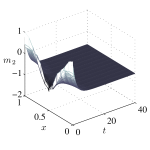
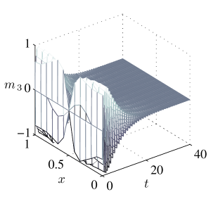
Figure 1: Magnetization in the uncontrolled Landau–Lifshitz equation moves from initial condition $\mathbf{{m}_{0}}(x)$, to the equilibrium $\mathbf{r_{0}}=(0,-0.6,0)$.

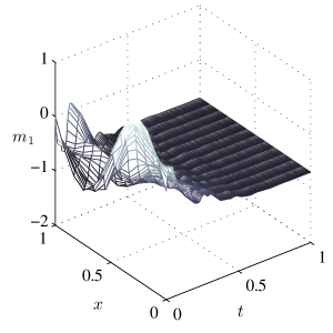
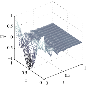
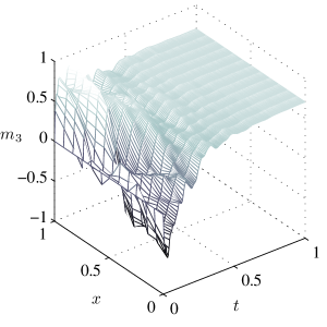
Figure 2: With a proportional control $(k=0.5)$, magnetization in the Landau–Lifshitz equation with a linear control moves from the initial condition $\mathbf{{m}_{0}}(x)$ to the specified equilibrium $\mathbf{r_{1}}=(-\frac{1}{\sqrt{2}},0,\frac{1}{\sqrt{2}}).$

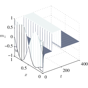
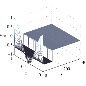
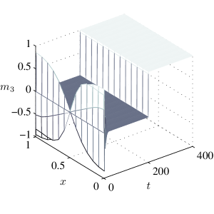
Figure 3: Steering magnetization between specified equilibria with a linear control. The uncontrolled magnetization moves from initial condition $\mathbf{{m}_{0}}$ to $\mathbf{r_{0}}=(0,-0.6,0)$. Proportional control $(k=0.5)$ with two successive values of $\mathbf{r}$ first forces the magnetization to $\mathbf{r_{2}}=(1,0,0)$ and then to $\mathbf{r_{3}}=(0,0,1)$.

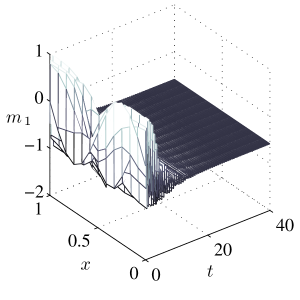
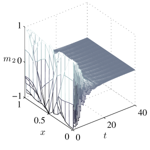
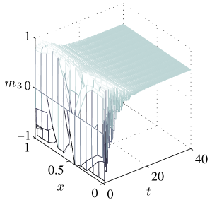
Figure 4: Magnetization in the Landau–Lifshitz equation with nonlinear control moves from the initial condition $\mathbf{{m}_{0}}(x)$ to the specified equilibrium $\mathbf{r_{1}}=(-\frac{1}{\sqrt{2}},0,\frac{1}{\sqrt{2}})$ with control parameter $k=10$.

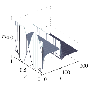
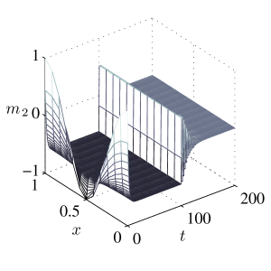
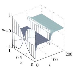
Figure 5: Magnetization in the Landau–Lifshitz equation moves from the initial condition $\mathbf{{m}_{0}}(x)$ to the equilibrium $\mathbf{r_{0}}=(0,-0.6,0)$ without a control. The control, $\mathbf{u}$ with $k=10$ is then applied to the equation nonlinearly and steers the dynamics to the specified equilibrium $\mathbf{r_{1}}=(-\frac{1}{\sqrt{2}},0,\frac{1}{\sqrt{2}})$.

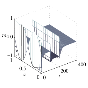
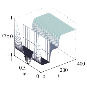
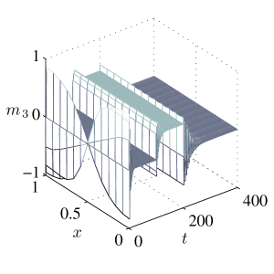
Figure 6: Magnetization in the Landau–Lifshitz equation moves from the initial condition $\mathbf{{m}_{0}}(x)$ to the equilibrium $\mathbf{r_{0}}=(0,-0.6,0)$ without a control. The control $\mathbf{u}$ with $k=10$ is then applied to the equation nonlinearly and steers the dynamics to the specified equilibrium $\mathbf{r_{1}}=(-\frac{1}{\sqrt{2}},0,\frac{1}{\sqrt{2}})$, and then to another equilibrium, $\mathbf{r_{4}}=(0,1,0)$.

References

• [1] L. Landau and E. Lifshitz, “On the theory of the dispersion of magnetic permeability in ferromagnetic bodies,” Ukrainian Journal of Physics, vol. 53, no. Special Issue, pp. 14–22, 2008.
• [2] A. Chow and K. A. Morris, “Hysteresis in the Landau–Lifshitz equation.,” in Proceedings of the American Control Conference, 2014.
• [3] K. Morris, “What is hysteresis?,” Applied Mechanics Reviews, vol. 64, no. 5, 2011.
• [4] A. Bensoussan, Representation and Control of Infinite Dimensional Systems. Birkhauser, 2007.
• [5] R. Curtain and H. Zwart, An introduction to Infinite-Dimensional Linear Systems Theory, vol. 21 of Texts in Applied Mathematics. Springer-Verlag, 1995.
• [6] I. Lasiecka and R. Triggiani, Control Theory for Partial Differential Equations: Continuous and Approximation Theories, vol. I. Cambridge University Press, 2000.
• [7] I. Lasiecka and R. Triggiani, Control Theory for Partial Differential Equations: Continuous and Approximation Theories, vol. II. Cambridge University Press, 2000.
• [8] K. A. Morris, “Control of systems governed by partial differential equations,” in Control Handbook (W. Levine, ed.), IEEE, 2010.
• [9] S. Noh, Y. Miyamoto, M. Okuda, N. Hayashi, and Y. K. Kim, “Control of magnetic domains in co/pd multilayered nanowires with perpendicular magnetic anisotropy,” Journal of Nanoscience and Nanotechnology, vol. 12, no. 1, pp. 428 – 432, 2012.
• [10] R. Wieser, E. Y. Vedmedenko, and R. Wiesendanger, “Indirect Control of Antiferromagnetic Domain Walls with Spin Current,” Physical Review Letters, vol. 106, no. 6, 2011.
• [11] G. Carbou and S. Labbe, “Stabilization of walls for nano-wires of finite length,” ESAIM, Control Optim. Calc. Var. (France), vol. 18, no. 1, pp. 1 – 21, 2012.
• [12] G. Carbou, S. Labbé, and E. Trélat, “Control of travelling walls in a ferromagnetic nanowire,” Discrete and Continuous Dynamical Systems. Series S, vol. 1, no. 1, pp. 51–59, 2008.
• [13] G. Carbou, S. Labbé, and E. Trélat, “Smooth control of nanowires by means of a magnetic field,” Communications on Pure and Applied Analysis, vol. 8, no. 3, pp. 871–879, 2009.
• [14] G. Carbou and S. Labbé, “Stability for walls in ferromagnetic nanowire,” in Numerical mathematics and advanced applications, pp. 539–546, Berlin: Springer, 2006.
• [15] G. Carbou and S. Labbé, “Stability for static walls in ferromagnetic nanowires,” Discrete Contin. Dyn. Syst. Ser. B, vol. 6, no. 2, pp. 273–290 (electronic), 2006.
• [16] R. Jizzini, “Optimal stability criterion for a wall in a ferromagnetic wire in a magnetic field,” Journal of Differential Equations, vol. 250, pp. 3349–3361, APR 15 2011.
• [17] S. Labbe, Y. Privat, and E. Trelat, “Stability properties of steady-states for a network of ferromagnetic nanowires,” J. Differ. Equ. (USA), vol. 253, no. 6, pp. 1709 – 28, 2012.
• [18] R. A. Jamal and K. A. Morris, “Linearized stability of partial differential equations with application to stabilization of the Kuramoto-Sivashinsky equation.” submitted, 2014.
• [19] R. al Jamal, A. Chow, and K. A. Morris, “Linearized stability analysis of nonlinear partial differential equations,” in Proceedings of the 21st International Symposium on Mathematical Theory of Networks and Systems, 2014.
• [20] W. Brown, Micromagnetics. No. 18 in Interscience Tracts on Physics and Astronomy, Wiley, 1963.
• [21] B. Guo and S. Ding, Landau-Lifshitz Equations, vol. 1 of Frontier Of Research with the Chinese Academy of Sciences. World Scientific, 2008.
• [22] T. Gilbert, “A phenomenological theory of damping in ferromagnetic materials,” IEEE Transactions on Magnetics, vol. 40, no. 6, pp. 3443 – 3449, 2004.
• [23] G. Carbou and P. Fabrie, “Regular solutions for Landau-Lifschitz equation in a bounded domain,” Differential Integral Equations, vol. 14, no. 2, pp. 213–229, 2001.
• [24] F. Alouges and A. Soyeur, “On global weak solutions for Landau-Lifshitz equations: existence and nonuniqueness,” Nonlinear Anal., vol. 18, no. 11, pp. 1071–1084, 1992.
• [25] A. Chow, Control of hysteresis in the Landau-Lifshitz Equation. PhD thesis, University of Waterloo, 2013.
• [26] B. Cullity and C. Graham, Introduction to Magnetic Materials. Wiley, second ed., 2009.
• [27] M. Lakshmanan, “The fascinating world of the landau-lifshitz-gilbert equation: an overview,” Phil. Tran. Royal Society A, vol. 369, pp. 1280–1300, 2011.
• [28] Z. H. Luo, B. Z. Guo, and O. Morgul, Stability and Stabilization of Infinite Dimensional Systems with Applications. Communications and Control Engineering, Springer, 1999.
• [29] T. Kato, “Nonlinear semigroups and evolution equations.,” J. Math. Soc. Japan, vol. 19, pp. 508–520, 508–520, 1967.
Refer to captionRefer to caption
Refer to caption