Agent-based model for the h-index – Exact solution

Abstract

Hirsch’s $h$-index is perhaps the most popular citation-based measure of scientific excellence. In 2013 G. Ionescu and B. Chopard proposed an agent-based model describing a process for generating publications and citations in an abstract scientific community. Within such a framework, one may simulate a scientist’s activity, and – by extension – investigate the whole community of researchers. Even though the Ionescu and Chopard model predicts the $h$-index quite well, the authors provided a solution based solely on simulations. In this paper, we complete their results with exact, analytic formulas. What is more, by considering a simplified version of the Ionescu-Chopard model, we obtained a compact, easy to compute formula for the $h$-index. The derived approximate and exact solutions are investigated on a simulated and real-world data sets.

1 Introduction

Since the 1999 seminal paper by Barabási and Albert BarabasiAlbert1999:preferential many methods that originally were developed in statistical physics have been successfully applied in a wide range of problems coming from diverse domains. Scientometrics, an area in which one is concerned with the quantitative characteristics of science and scientific research, is one of such domains. Recently, different authors studied – among others – the long term prediction of scientific success Wang2013:Quantifying , impact that an affiliation change has on a scientist’s productivity Deville2014:career , or production and consumption of the knowledge in physics ZhangetAll2013:physics ; Mazloumian2013:foodweb . However, historically main efforts were focused on the study of the structure of citation networks Redner1998:citationdist ; Golosovsky2013:JStatPhys ; Jeong ; Eom2011:citationdynamisc , and the reproduction of their degree distributions Eom2011:citationdynamisc ; Krapivsky2000:network ; Newman2011:clustering ; GolosovskyPRL . Starting from the de Solla Price seminal work deSollaPrice1965 it is a known fact that citation networks arise due to the preferential attachment rule BarabasiAlbert1999:preferential . This process, well known in complex network analysis Jeong ; Krapivsky2000:network ; Newman2011:clustering , was studied from the point of view of citation networks Golosovsky2013:JStatPhys ; Eom2011:citationdynamisc ; GolosovskyPRL ; WangPhysA1 ; WangPhysA2 , where it is also known as the rich get richer rule or the Matthew effect Perc . Different variations of the classical, linear, preferential attachment (see Krapivsky2000:network or Table 1 in Golosovsky2013:JStatPhys ) were considered, but to the best of our knowledge there is a lack of models in the literature which concern the $h$-index (except IonescuChopard , which is described in Sec. 2).

The $h$-index proposed in 2005 by J.E. Hirsch Hirsch2005:hindex is the most popular citation-based measure of scientific excellence. Even though this data fusion tool was already studied in the 1940s (compare the notion of the Ky Fan metric Fan1943:metric and also the Sugeno integral, see, e.g., GagolewskiMesiar2014:Integrals ), it may be conceived as a turning point in the history of scientometrics. The idea standing behind the Hirsch index is to measure not only the overall quality of a scientist’s output (most often expressed by the number of citations that each individual paper received), but also its size. Thus, it may be understood as a measure of both productivity and impact of a researcher (or an institution). More formally, let us assume that we are given a list $\mathbf{S}=(S_{1},\dots,S_{n})\in\mathbb{N}_{0}^{n}$, where $S_{i}$ denotes the number of citations to the $i$-th paper. If $S_{(n)}\geq 1$, the Hirsch index is given by the formula:

$$h\textrm{-index}=\max{\left\{h=1,\dots,n:\ S_{(n-h+1)}\allowbreak\geq h\right\}},$$

where $S_{(n-h+1)}$ denotes the $(n-h+1)$-th order statistic of $\mathbf{S}$. Moreover, if $S_{(n)}=0$, then $h\textrm{-index}=0$. Intuitively, an author has his/her $h$-index equal to $H$, if $H$ of her/his $n$ papers have at least $H$ citations each, and the other $n-H$ papers have at most $H$ citations each.

There were a few papers devoted to the stochastic properties of the $h$-index in some simple probabilistic models, see EggheRousseau2006:informetrich ; vanRaan2006:147chem ; Burrell2007:hstochastic ; Gagolewski2012:smps ). Recently, Ionescu and Chopard in IonescuChopard considered a publication-citation process in an abstract scientific community which was described by a multi-agent model. Such a model consists of a scientist producing new papers, giving citations to the already published papers (including his/her own ones), and receiving citations from the community. This bottom-up approach allows to simulate a single scientist’s activity as well as to investigate the whole community of researchers. What was very inspiring for us is the fact, that Fig. 3. in deSollaPrice1965 is a perfect illustration of the mechanism of Ionescu-Chopard model, but this de Solla Price article was published almost $50$ years before Ionescu and Chopard paper. Nevertheless, it turns out that their approach predicts quite well the $h$-index from bibliometric data. However, its authors did not provide an analytic form of a solution to their model, relying only on Monte Carlo simulations instead. In the current work we present an exact solution to that model as well as its simplification and an application on real-world data.

The paper is organized as follows. In Sec. 2 the agent-based model proposed by Ionescu and Chopard (referred to as the IC model) is described in very detail. Sec. 3 presents theoretical results concerning exact formulas for vectors of citations and the results of comparative simulation studies. In Sec. 4 a simplified model is proposed. Next, in Sec. 5 the results of an empirical analysis concerning all investigated approximations of the $h$-index are presented. Finally, Sec. 6 concludes the paper.

2 The IC single-scientist model

In 2013 Ionescu and Chopard IonescuChopard introduced a multi-agent model to describe a publication-citation generation process in an abstract scientific community. Their approach consists of a scientist producing new papers, giving citations to his own and other already published papers, and receiving citations from the community. The model is based on a preferential attachment rule BarabasiAlbert1999:preferential , which was observed in many real-world systems BarabasiAlbert1999:preferential ; Jeong . As we mentioned before, preferential attachment rule is strongly connected with the so-called Matthew effect Perc : highly cited articles are more eagerly cited by other authors than lowly cited ones. More precisely, the probability of adding new citations to a paper is proportional to the number of citations it has already obtained.

2.1 Simulation description

Unlike in the case of various well-known models for constructing citation networks Eom2011:citationdynamisc ; GolosovskyPRL ; WangPhysA1 ; WangPhysA2 , the IC model focuses not on the overall structure of a citation network but only on the node degree distribution, i.e., on the number of citations of papers written by one author. Its aim is to approximate citation scores for each published paper of a given author, i.e., an $N$ dimensional vector $S=(S_{1},\ldots,S_{N})$, where $S_{k}$ denotes the number of citations of the $k$-th paper. By definition, this shall be based solely on the number $N$ of papers he/she published as well as the total number $M$ of citations that his/her papers obtained. Moreover, we assume that citations to each paper $S_{k}$ are of two kinds: external $X_{k}$ and internal (self) ones $Y_{k}$, thus $S_{k}=X_{k}+Y_{k}$.

The simulation of interest is an iterative process. We start with an initial number of papers $N_{0}$, none of which is cited. During each iteration we add a new paper to the collection and distribute both self and external citations to the existing papers according to the preferential attachment rule. We give a fixed number of $p$ internal and $q$ external citations to the $k$-th paper with probability of:

$$p_{k}=\frac{X_{k}+1}{\sum\limits_{l=1}^{n}X_{l}+n},\quad k=1,\ldots,n.$$ (1)

Due to the form of the given probability distribution, in IonescuChopard it is assumed that only external citations are taken into account when assigning the new ones. Self citations do not influence a paper’s importance. Once the fixed number $N$ of published papers is reached, the process goes on, but only $q$ external citations are being granted during each step. The simulation ends as soon as the total number of citations $M$ has been distributed.

Simulation steps in the IC model

Let us now formalize the aforementioned procedure. Such a detailed introduction is crucial for solving the model: the simulation may end up on different stages depending on parameter values. The IC model is based on the following input parameters:

1. the number of papers $N\in\mathbb{N}$,

2. the total number of citations $M\in\mathbb{N}$,

3. the number of self citations added in each step $p\in\mathbb{N}$,

4. the number of external citations added in each step $q\in\mathbb{N}$ and

5. the initial number of papers with no citations at the beginning $N_{0}\in\mathbb{N}$.

The initial values for sequences $\mathbf{X}$ and $\mathbf{Y}$ are given by $X_{1}^{(0)}=0,\ldots,X_{N}^{(0)}=0$ and $Y_{1}^{(0)}=0,\ldots,Y_{N}^{(0)}=0$. Values $X_{k}^{(t)}$ and $Y_{k}^{(t)}$ denote the number of external and self citations, respectively, of the $k$-th paper in the $t$-th iteration. Before the $k$-th paper is published, its citation counts are set to $0$. Thus, $X_{k}^{(t)}=Y_{k}^{(t)}=0$ for $k>t$. Nevertheless, please note that this assumption has no impact on further derivations, as it is well-known that papers with no citations do not influence the $h$-index value.

The simulation consists of the three following phases.

Phase 0.

Firstly, we initialize the variables $X_{1},\dots,X_{N_{0}}$ and $Y_{1},\dots,\allowbreak Y_{N_{0}}$, and set $t=N_{0}$. In the first step of the next phase we are going to distribute citations across the first $N_{0}$ articles. In other words, the considered author has already published her/his first $N_{0}$ articles and is waiting for citations. Two cases are possible:

• $N_{0}\geqslant N$ $\rightarrow$ the author published less than $N_{0}$ papers. In such a case, the simulation ends before going to phase (I), even though it is possible that there are still citations left to be distributed. We could try going straight to phase (II) and distribute these citations, yet it would not increase the precision of the $h$-index estimation significantly (due to the fact that $N_{0}$ is small). On the other hand, this would unnecessarily complicate the formulas for $X_{k}$ and $Y_{k}$.

• $N_{0}<N$ $\rightarrow$ there are enough papers and citations to go to phase (I).

Phase (I)

For each $t=N_{0}+1,\ldots,\min\{N,\lfloor\frac{M}{p+q}\rfloor+N_{0}\}$, we distribute $q$ external and $p$ self citations according to the preferential attachment rule given by Eq. (1):

$$X_{k}^{(t)} =X_{k}^{(t-1)}+\sum\limits_{j=0}^{q}j\cdot\mathbb{P}(X_{k}^{(t-1)}\rightarrow X_{k}^{(t-1)}+j),$$ (2)

$$Y_{k}^{(t)} =Y_{k}^{(t-1)}+\sum\limits_{j=0}^{p}j\cdot\mathbb{P}(Y_{k}^{(t-1)}\rightarrow Y_{k}^{(t-1)}+j).$$ (3)

When phase (I) comes to an end (which means that the author has already published all her/his works and obtained all self citations), the three following cases are possible:

• $\frac{M}{p+q}+N_{0}=N$ $\rightarrow\,$ simulation ends with no citations to distribute left,

• $\frac{M}{p+q}+N_{0}<N$ $\rightarrow\,$ simulation ends, even if there are possibly up to $p+q-1$ undistributed citations left. In this case we could distribute such leftover citations, yet it would not increase the precision of the $h$-index estimation significantly and would unnecessarily complicate the formulas for $X_{k}$ and $Y_{k}$,

• $\frac{M}{p+q}+N_{0}>N$ $\rightarrow\,$ simulation does not end, there are still citations to be distributed. We go to phase (II).

Phase (II)

For each $t=N+1,\ldots,\lfloor\frac{M-(N-N_{0})(p+q)}{q}\rfloor+N$, we shall distribute only the external citations among the already published $N$ papers:

$$X_{k}^{(t)} =X_{k}^{(t-1)}+\sum\limits_{j=0}^{q}j\cdot\mathbb{P}(X_{k}^{(t-1)}\rightarrow X_{k}^{(t-1)}+j),$$ (4)

$$Y_{k}^{(t)} =Y_{k}^{(t-1)}.$$

When phase (II) comes to an end, two situations are possible:

• $\left(M-(N-N_{0})(p+q)\right)\ \mathrm{mod}\ q=0$ $\rightarrow\,$ simulation ends, no citations to distribute left,

• $\left(M-(N-N_{0})(p+q)\right)\ \mathrm{mod}\ q\neq 0$ $\rightarrow\,$ simulation ends, even though there are possibly up to $q-1$ undistributed citations left. The reason to abandon the leftover citations distribution is the same as in phase (I).

3 Exact formulas for citation vectors

Let us now present the exact formulas for $X_{k}^{(t)}$ and $Y_{k}^{(t)}$ derived for the IC model.

3.1 External citations

Please notice that the sums in Eqs. (2) and (4) are in fact the expected values of random variables from binomial distributions $\mathrm{Bin}(q,p_{k,t})$ and $\mathrm{Bin}(q,\tilde{p}_{k,t})$, respectively, where probabilities $p_{k,t}$, $\tilde{p}_{k,t}$ are given by:

$$p_{k,t}=\mathbb{P}(X_{k}^{(t-1)}\rightarrow X_{k}^{(t-1)}+1)=$$ (5)

$$= \mathbb{P}(Y_{k}^{(t-1)}\rightarrow Y_{k}^{(t-1)}+1)=\begin{cases}\frac{X_{k}^{(t-1)}+1}{\sum\limits_{l=1}^{t}X_{l}^{(t-1)}+t},&k\leqslant t,\\ 0,&k>t,\end{cases}$$

and

$$\tilde{p}_{k,t} =\mathbb{P}(X_{k}^{(t-1)}\rightarrow X_{k}^{(t-1)}+1)$$

$$=\frac{X_{k}^{(t-1)}+1}{\sum\limits_{l=1}^{N}X_{l}^{(t-1)}+N},\textrm{ for }k\leqslant N,\,t>N.$$

The value of $X_{k}$ in the $t$-th step can be written as:

$$X_{k}^{(t)} =\left\{\begin{array}[]{ll}X_{k}^{(t-1)}+qp_{k,t},&t\leqslant N,\\ X_{k}^{(t-1)}+q\tilde{p}_{k,t},&t>N,\end{array}\right.$$ (8)

$$=\left\{\begin{array}[]{ll}X_{k}^{(t-1)}+\frac{q(X_{k}^{(t-1)}+1)}{\sum\limits_{l=1}^{t}X_{l}^{(t-1)}+t},&t\leqslant N,\\ X_{k}^{(t-1)}+\frac{q(X_{k}^{(t-1)}+1)}{\sum\limits_{l=1}^{N}X_{l}^{(t-1)}+N},&t>N.\end{array}\right.$$

The sums in the denominators are equal to

$$\sum\limits_{l=1}^{\min\{t,N\}}X_{l}^{(t-1)}=q(t-1-N_{0}).$$

Therefore,

$$X_{k}^{(t)}+1 =\left\{\begin{array}[]{ll}(X_{k}^{(t-1)}+1)\left(1+\frac{q}{t(q+1)-q(N_{0}+1)}\right),&t\leqslant N,\\ (X_{k}^{(t-1)}+1)\left(1+\frac{q}{tq+N-q(N_{0}+1)}\right),&t>N,\end{array}\right.$$

and now this recurrence relation can be solved easily. We wish to find $X_{k}=X_{k}^{(t_{\max})}$, where the value of $t_{\max}$ depends on whether the simulation stops in phase (I) or (II). When solving the recurrence equations we continue until reaching $X_{k}^{(k-1)}=0$ or $X_{k}^{(N_{0})}=0$. As a consequence, if $t_{\max}\leqslant N$, then we obtain:

$$X_{k}=\prod\limits_{l=t_{\min}}^{t_{\max}}\left(1+\frac{q}{l(q+1)-q(N_{0}+1)}\right)-1,$$

and if $t_{\max}>N$, then it holds:

$$X_{k}=\allowbreak \prod\limits_{l=t_{\min}}^{N}\left(1+\frac{q}{l(q+1)-q(N_{0}+1)}\right)\times$$

$$\times \prod\limits_{l=N+1}^{t_{\max}}\left(1+\frac{q}{lq+N-q(N_{0}+1)}\right)-1,$$

where

$$t_{\min} =\max\{N_{0}+1,k\},$$

$$t_{\max} =\left\{\begin{array}[]{ll}\lfloor\frac{M}{p+q}\rfloor+N_{0},&\textrm{ if }\lfloor\frac{M}{p+q}\rfloor+N_{0}\leqslant N,\\ \lfloor\frac{M-(N-N_{0})(p+q)}{q}\rfloor+N_{0},&\textrm{ if }\lfloor\frac{M}{p+q}\rfloor+N_{0}>N.\end{array}\right.$$

Please note that we can simplify the above formula by relying on the notion of the $\Gamma$ function. Firstly, observe that:

$$\prod\left(1+\frac{q}{l(q+1)-q(N_{0}+1)}\right)=\frac{\prod\left(l-\alpha_{1}\right)}{\prod\left(l-\beta_{1}\right)},$$

$$\prod\left(1+\frac{q}{lq+N-q(N_{0}+1)}\right)=\frac{\prod\left(l-\alpha_{2}\right)}{\prod\left(l-\beta_{2}\right)},$$

where:

$$\alpha_{1}=\frac{qN_{0}}{q+1},\quad\beta_{1}=\frac{q(N_{0}+1)}{q+1},$$

$$\alpha_{2}=\frac{qN_{0}-N}{q},\quad\beta_{2}=\alpha_{2}+1.$$

Moreover,

$$l-\alpha=\frac{\Gamma(l-\alpha+1)}{\Gamma(l-\alpha)},$$

and

$$\prod\limits_{l=t_{1}}^{t_{2}}(l-\alpha)=\frac{\Gamma(t_{2}-\alpha+1)}{\Gamma(t_{1}-\alpha)}.$$

Hence, the formula for $X_{k}$ can be written as:

$$X_{k}=\frac{t_{\max}-\alpha_{2}}{N-\alpha_{2}}\frac{\Gamma(N-\alpha_{1}+1)\Gamma(t_{\min}-\beta_{1})}{\Gamma(t_{\min}-\alpha_{1})\Gamma(N-\beta_{1}+1)}-1,$$ (10)

with:

$$t_{\min} =\max\{N_{0}+1,k\},$$

$$t_{\max} =\left\{\begin{array}[]{ll}\lfloor\frac{M}{p+q}\rfloor+N_{0},&\textrm{ if }\lfloor\frac{M}{p+q}\rfloor+N_{0}\leqslant N,\\ \lfloor\frac{M-(N-N_{0})(p+q)}{q}\rfloor+N_{0},&\textrm{ if }\lfloor\frac{M}{p+q}\rfloor+N_{0}>N,\end{array}\right.$$

$$\alpha_{1} =\frac{qN_{0}}{q+1},\quad\beta_{1}=\frac{q(N_{0}+1)}{q+1},\quad\alpha_{2}=\frac{qN_{0}-N}{q}.$$

The above simplification gives a more elegant representation of $\mathbf{X}$. However, it is worth noting that the product form is more computationally stable than calculating gamma functions for large arguments. Due to this fact in our simulations we use the product form. Nevertheless, both representations enable us to compute the elements of $\mathbf{X}$ significantly faster than in the case of the simulation procedure presented in IonescuChopard .

3.2 Self citations

Similarly as in the previous subsection, we can solve the equation for self citations distribution. Basing on Eqs. (3) and (5), we have:

$$Y_{k}^{(t)} =Y_{k}^{(t-1)}+pp_{k,t}$$

$$=Y_{k}^{(t-1)}+\frac{p(X_{k}^{(t-1)}+1)}{q(t-1-N_{0})+t}$$

$$=Y_{k}^{(t-1)}$$

$$\quad+\frac{p}{q(t-1-N_{0})+t}\prod\limits_{l=t_{\min}}^{t-1}\Big{(}1+\frac{q}{q(l-1-N_{0})+l}\Big{)}$$

$$=\sum\limits_{i=t_{\min}+1}^{t}\frac{p}{q(i-1-N_{0})+i}\prod\limits_{l=t_{\min}}^{i-1}\Big{(}1+\frac{q}{q(l-1-N_{0})+l}\Big{)}$$

$$\quad+\frac{p}{(t_{\min}-1-N_{0})+t_{\min}}.$$

We would like to find $Y_{k}=Y_{k}^{(s_{\max})}$, and due to the fact that here we always end up in phase (I), $s_{\max}$ is equal to:

$$s_{\max}=\min\{N,\lfloor\frac{M}{p+q}\rfloor+N_{0}\}.$$

Hence,

$$Y_{k} =\sum\limits_{i=t_{\min}+1}^{s_{\max}}\frac{p}{q(i-1-N_{0})+i}\prod\limits_{l=t_{\min}}^{i-1}\left(1+\frac{q}{q(l-1-N_{0})+l}\right)$$

$$+\frac{p}{(t_{\min}-1-N_{0})+t_{\min}}.$$

Also, the formula for $Y_{k}$ may be simplified as follows:

$$Y_{k} =\sum\limits_{i=t_{\min}+1}^{s_{\max}}\frac{p}{q(i-1-N_{0})+i}\frac{\Gamma(i-\alpha)\Gamma(t_{\min}-\alpha)}{\Gamma(t_{\min}-\beta)\Gamma(i-\beta)}$$

$$+\frac{p}{(t_{\min}-1-N_{0})+t_{\min}},$$ (11)

where

$$\alpha=\frac{qN_{0}}{q+1},\quad\beta=\frac{q(N_{0}+1)}{q+1}.$$

3.3 Non-integer values of $p$ and $q$

The authors of the IC model mention in IonescuChopard that, given non-integer values of $p$ and $q$, one distributes:

$$p^{\prime}=\left\{\begin{array}[]{ll}\lceil p\rceil&\text{with probability }1-(\lceil p\rceil-p)\\ \lceil p\rceil-1&\text{with probability }(\lceil p\rceil-p)\\ \end{array}\right.$$

self-citations as well as:

$$q^{\prime}=\left\{\begin{array}[]{ll}\lceil q\rceil&\text{with probability }1-(\lceil q\rceil-q)\\ \lceil q\rceil-1&\text{with probability }(\lceil q\rceil-q)\\ \end{array}\right.$$

citations given by the scientific community. Therefore, as with probabilities of $1-(\lceil p\rceil-p)$ and $1-(\lceil q\rceil-q)$ the average number of self- and external citations is equal to $p$ and $q$, respectively.

Let us consider $X_{k}^{(t)}$ and let the second summand in Eq. (8) be denoted as:

$$\mathbb{E}(Q_{k}^{t})=\left\{\begin{array}[]{ll}qp_{k,t}&t\leqslant N,\\ q\tilde{p}_{k,t}&t>N,\\ \end{array}\right.$$

where the number of external citations to the $k$-th paper obtained at time $t$, $Q_{k}^{t}$ , follows the $\mathrm{Bin}(q,p_{k,t})$ distribution for $t\leqslant N$ and the $\mathrm{Bin}(q,\tilde{p}_{k,t})$ distribution for $t>N$. Moreover,

$$\mathbb{E}(Q_{k}^{t}|q^{\prime})=\left\{\begin{array}[]{ll}\lceil q\rceil p_{k,t}&\text{with probability }1-(\lceil q\rceil-q),\\ (\lceil q\rceil-1)p_{k,t}&\text{with probability }(\lceil q\rceil-q).\\ \end{array}\right.$$

Taking into account the distribution of $q^{\prime}$, we have that:

$$\mathbb{E}(Q_{k}^{t}) = \mathbb{E}(Q_{k}^{t}|q^{\prime}=\lceil q\rceil)\,\mathbb{P}(q^{\prime}=\lceil q\rceil)$$

$$+ \mathbb{E}(Q_{k}^{t}|q^{\prime}=\lceil q\rceil-1)\,\mathbb{P}(q^{\prime}=\lceil q\rceil-1).$$

Therefore, Eq. (8) is now of the form:

$$X_{k}^{(t)} =X_{k}^{(t-1)}+\lceil q\rceil p_{k,t}(1+q-\lceil q\rceil)$$

$$+(\lceil q\rceil-1)p_{k,t}(\lceil q\rceil-q)$$

$$=X_{k}^{(t-1)}+(\lceil q\rceil+1+q-\lceil q\rceil-1)p_{k,t}$$

$$=X_{k}^{(t-1)}+qp_{k,t}.$$

By relying on a similar reasoning we obtain:

$$Y_{k}^{(t)} =Y_{k}^{(t-1)}+\lceil p\rceil p_{k,t}(1+p-\lceil p\rceil)$$

$$+(\lceil p\rceil-1)p_{k,t}(\lceil p\rceil-p)$$

$$=Y_{k}^{(t-1)}+pp_{k,t}.$$

It is easily seen that final form of the result is the same as for the formulas for integer $p$ and $q$.

3.4 Overall number of citations and the h-index

Once we have determined the formulas for external $X_{k}$ and self $Y_{k}$ citations corresponding to the Ionescu and Chopard model, the only action left to estimate $h$-index is just to sum them up. One sees that both $X_{k}$ and $Y_{k}$ are nondecreasing, so $S_{k}=X_{k}+Y_{k}$ is also nondecreasing and thus:

$$h_{\mathrm{exact}}=\max\{k:S_{k}\geqslant k\}.$$

3.5 Comparative simulation study

Let us now briefly compare the estimates of the $h\textrm{-index}$ obtained with the IC model (denoted as $h_{\mathrm{IC}}$) and $h_{\mathrm{exact}}$, i.e., the ones that are based on Eq. (10) and Eq. (11). We consider the vector of citations of J.E. Hirsch himself. The data were gathered on July 30, 2015 from the Scopus database. The vector consists of the total number of $M=13480$ citations and the total number of $N=205$ publications. The $h$-index of Hirsch is equal to $52$.

According to IonescuChopard , parameters $p$ and $q$ giving the best global agreement between the IC model and the original $h$-index are equal to 1 and 2, respectively. However, the authors also stated that $p$ and $q$ can be tuned up in such a way that almost any scientific profile can be fit well. In the case of the $h$-index of Hirsch, we found out that $p=1$ and $q=3$ gives a reasonable agreement, while for $q=2$ the final $h$-index is overestimated. Please note that the model is stochastic in its nature and its results vary across different simulation runs, even for the same values of $p$, $q$, $M$ and $N$. Therefore, for the purpose of a sensible comparison, we analyzed 1000 samples for $p=1$, $q=1,2,\dots,10$ and $N_{0}=p+q$. The $h_{\mathrm{IC}}$ distribution estimates are presented in Fig. 1 in a form of box-and-wiskers plots Additionally, the $h_{\mathrm{exact}}$ and the $h$-index obtained by averaging the citation vectors as generated by the IC model are indicated. We may observe a high agreement between $h_{\mathrm{IC}}$ computed on an averaged citation vector and $h_{\mathrm{exact}}$ (the largest difference between these two estimates, i.e., $|h_{\mathrm{IC}}-h_{\mathrm{exact}}|$ is equal to 1).

Figure 1: Boxplots for the distribution of the $h$-index of Hirsch as estimated via the IC model. Additionally, the $h$-index computed according to citation vectors obtained via Eqs. (10) and (11) is marked with $\bigtriangleup$ and the $h$-index obtained from averaged citation vectors from the IC model by $\boldsymbol{\times}$.

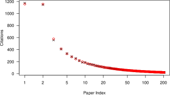
(a) Vector of external citations $X$.

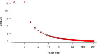
(b) Vector of self citations $Y$.

Figure 2: Step plots of vectors of external $X$ and self citations $Y$ obtained from the IC model, depicted by $\boldsymbol{\times}$, and Eqs. (10) and (11), depicted by $\circ$.

As it was stated in IonescuChopard , the initial number of publications $N_{0}$ should be small enough so as to not influence the rest of the process, but large enough in order to provide enough papers to cite in the first iteration. The authors suggest to choose $N_{0}=p+q$. In order to assess the influence of this parameter on $h_{\mathrm{IC}}$ and $h_{\mathrm{excat}}$, we analyze $N_{0}$ varying from $1$ to $50$, for $p=1$ and $q=2$. Please note that $N_{0}=50$ is nearly 25% of all the Hirsch’s publication count. For the IC model, we perform 1000 runs and average the obtained values: $\mathsf{AVR}(h_{\mathrm{IC}})$ denotes the mean of $h_{\mathrm{IC}}$ obtained in each run and $\mathrm{sd}$ its standard deviation, while $h_{\mathrm{IC}}(\mathsf{AVR})$ denotes the $h$-index computed on an averaged citation vector from the IC model. The results presented in Table 1 suggest that there is no significant difference between $N_{0}=1,2$ and $N_{0}=p+q=3$ in this case. Therefore, one may choose $N_{0}=1$ and if $N=1$ and $M>0$, simply assign the $h$-index equal to $1$.

Table 1: Aggregated results of 1000 runs of the IC model for $p=1$, $q=2$ and $N_{0}\in\{1,\dots,10,15,20,25,50\}$, where $\mathsf{AVR}(h_{\mathrm{IC}})$ denote the mean $h_{\mathrm{IC}}$, sd its standard deviation, $h_{\mathrm{IC}}(\mathsf{AVR})$ the $h$-index computed on an averaged citation vector from IC model and $h_{exact}$ – the $h$-index obtained via analytical formulas.

$N_{0}$	$\mathsf{AVR}(h_{\mathrm{IC}})$	$sd$	$\mathsf{AVR}(h_{\mathrm{IC}})\pm sd$	$h_{\mathrm{IC}}(\mathsf{AVR})$	$h_{\mathrm{exact}}$
1	56.19	2.47	(53.71;58.66)	54	54
2	56.52	2.35	(54.17;58.87)	54	54
3	56.73	2.36	(54.38;59.09)	54	54
4	57.04	2.38	(54.66;59.42)	55	55
5	57.34	2.30	(55.04;59.64)	55	55
6	57.51	2.30	(55.21;59.81)	55	55
7	57.81	2.37	(55.44;60.18)	56	56
8	58.21	2.27	(55.94;60.48)	57	56
9	58.43	2.34	(56.08;60.77)	56	56
10	58.63	2.43	(56.2;61.07)	57	56
15	59.70	2.33	(57.36;62.03)	58	58
20	60.85	2.29	(58.56;63.14)	60	60
25	61.79	2.30	(59.49;64.09)	61	62
50	65.23	2.30	(62.93;67.53)	71	71

Fig. 2 presents the step plots of vectors of external citations $\mathbf{X}$ (a) and self citations $\mathbf{Y}$ (b) obtained from the averaged (over 1000 runs) IC model as well as Eq. (10), (11). The sum of squared differences between the simulated and analytical results are equal, respectively, 7.22 and 0.002. The real value of the $h$-index of Hirsch is equal to $52$ and the estimated values (for parameters $p=1$ and $q=2$) are equal to $h_{\mathrm{IC}}(\mathsf{AVR})=54$ and $h_{\mathrm{exact}}=54$.

4 A simplification of the IC model

Please note that the exact solution to the IC model, i.e., Eqs. (10) and (11), gives an analytical expression of the very intuitive and reasonable simulation setup as proposed by Ionescu and Chopard. Nevertheless, as the form of the derived formulas is quite complicated, their intuitive interpretation is difficult.

Let us recall that the IC model is based on an assumption that only external citations are taken into account when assigning new ones (due to the form of the probability distribution given by Eq. (1)). Moreover, during the simulation study, as it was also stated in IonescuChopard , we observed that the parameter $p$ has no significant influence on the outcoming $h$-index. Hence, in this section we reduce the number of parameters, which leads to a significant simplification of the model.

Let us employ the following assumptions:

1. We assume $N_{0}=0$, so the first paper starts to gain citations just after its publication.

2. We consider only one vector $\mathbf{X}$, which means that we take into account all the citations together without distinguishing between external and self citations.

The number of simulation parameters is decreased to only two: $q$, which is the number of citations given in each iteration and $T$, which is number of simulation steps. Similarly as in Sec. 3 let us write the recurrence relation for $X_{k}^{(t)}$:

$$X_{k}^{(t)} =X_{k}^{(t-1)}+\frac{q(X_{k}^{(t-1)}+1)}{\sum\limits_{l=1}^{t}X_{l}^{(t-1)}+t},\;\;\; k=1,\,\dots,\,t,$$

$$X_{k}^{(t)} =0,\;\;\; k=t+1,\,\dots,\,T,$$

which may be expressed as:

$$X_{k}=X_{k}(T)=\prod_{l=k}^{T}\frac{l}{l+q/(q+1)}-1,$$ (12)

which may be further simplified as:

$$X_{k}=\frac{\Gamma(T+1)}{\Gamma(T+1-q/(q+1))}\frac{\Gamma(k-q/(q+1))}{\Gamma(k)}-1.$$ (13)

Eq. (13) is the exact solution of our simplified version of the model, but the following asymptotic relation:

$$\lim_{t\rightarrow\infty}\frac{\Gamma(t+\alpha)}{\Gamma(t)t^{\alpha}}=1,$$

allows us to obtain the approximation of $X_{k}$ as:

$$X_{k}\approx\frac{\Gamma(T+1)}{\Gamma(T+1)(T+1)^{-\alpha}}\frac{\Gamma(k)k^{-\alpha}}{\Gamma(k)}-1=\left(\frac{T+1}{k}\right)^{\alpha}-1,$$

where $\alpha=q/(q+1)$.

Even with our exact solution finding the compact formula for the $h$-index seems untraceable. Fortunately, for the simplification of the IC model, an observation that $X_{k}$ is an increasing function of $k$ leads to:

$$h=\left(\frac{T+1}{h}\right)^{\alpha}-1,$$

which is equivalent to:

$$(h+1)h^{\alpha}=\left(T+1\right)^{\alpha}.$$ (14)

One can show that for every $T>0$ and $\alpha\in(0,1)$ Eq. (14) has always exactly one solution, which is the $h$-index.

5 Real data evaluation

In this section we perform an empirical analysis of exemplary citation vectors gathered from Elsevier’s Scopus (see Gagolewski2011:CITAN for the detailed description of the data set). Please note that the whole data set includes citation vectors corresponding to 16282 authors. Nevertheless, about 78% of all the vectors are of length one (among them ca. 32% represent a single uncited paper). This is typical to bibliometric data sets, which consist of a high number of short vectors. Moreover, since it is observed that all the vectors are skewed, usually to model them distributions like exponential or Pareto type II (Lomax) are used, (e.g., compare BarczaTelcs2009:paretoimplyh ; Glanzel2008:hconcatenation ; Glanzel2008:statbibh ). Table 2 presents basic sample statistics for the Scopus data set.

Table 2: Basic sample statistics (the Scopus data set) of the number of published papers by an author (N), total number of citations he/she received (M), number of citations to his/her most (max) and least (min) frequently cited paper.

	N	M	max	min
Min.	1	0	0	0
1st Qu.	1	0	0	0
Median	1	3	3	1
Mean	1.67	13.53	9.10	5.72
3rd Qu.	1	11	9	5
Max.	129	2396	836	836

For the sake of clarity of the results presented in this paper, a subset of 100 randomly chosen authors has been selected. In order to assess the quality of the proposed approximation we choose vectors of length greater than or equal to 20 (in total number of 69) and from the vectors of length smaller than 20 we randomly choose 31 with uniform distribution. Basic sample statistics of the selected sample are presented in Table 3.

Table 3: Basic sample statistics of the selected sample from the Scopus data set.

	N	M	max	min
Min.	1	0	0	0
1st Qu.	6	45.75	19.50	0
Median	21.50	207.50	36	0
Mean	26.79	369.60	76.36	1.34
3rd Qu.	31.75	486.20	102	0
Max.	129	2396	636	20

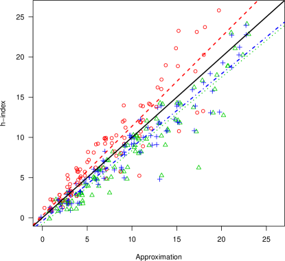
Figure 3: Comparison of the $h$-index and its approximations on a Scopus data set. The black continuous line is identity, so ideally all the points should overlie this line. The points depicted with $\circ$ correspond to values given by the $h$-index estimated from the exact solution of the IC simulation with parameters $N_{0}=1,p=1,q^{\prime}=2$, where only the vector of external citations was taken into account, i.e., one that is based on Eq. (10), the points marked with $+$ correspond to the estimate of the $h$-index that is based only on a vector of external citations (Eq. (12)) with parameter $q^{\prime\prime}=3$, while the points marked with $\bigtriangleup$ correspond to the approximation given by Eq. (14) with also $q^{\prime\prime}=3$. The dotted lines of corresponding color, depicted as $\boldsymbol{---}$, $\boldsymbol{-\cdot-\cdot-}$ and $\boldsymbol{\cdot\cdot\cdot\cdot\cdot}$, are the least squares fit of the $h$-index values and considered approximations, respectively.

In Fig. 3 there are presented the approximated values of $h$-index as a function of real values from considered data. Please note that the mean squared difference between the estimated values and the $h$-index equals to 6.15, 6.45 and 4.14, respectively for the estimates based on Eq. (10), Eq. (14) and Eq. (12).

Please note that in the case of Hirsch himself, considered in Sec. 3.5, the approximations of the $h$-index are equal to $51.99\approx 52$ for approximation given by Eq. (14) and $52$ for approximation based on Eq. (12). The obtained estimates of the Hirsch $h$-index for various values of parameter $q$ are presented in Table 4. Please note that by an appropriate selection of the parameter we were able to recreate the value of his $h$-index. Moreover, Fig. 4 depicts its predicted growth dynamic over each iteration. We see that our simplification does not predict the $h$-index worse than the original simulation. However, one should be aware that the approximate $h$-$\mathrm{index}$ given by Eq. (14) is not necessarily an integer value (compare Fig. 3 and Table 4). This should be taken into account in analysis of real data sets: if needed, e.g., proper rounding can be applied.

Table 4: The approximations of the Hirsch $h$-index calculated via Eq. (14) and based on Eq. (12) for various parameters $q$.

$q$	Eq. (14)	Rounded values of Eq. (14)	Eq. (12)
1	23.14	23	23
1.5	34.75	35	35
2	44.27	44	44
2.5	51.99	52	52
3	58.30	58	58
3.5	63.52	64	63
4	67.91	68	68
4.5	71.62	72	72
5	74.82	75	75

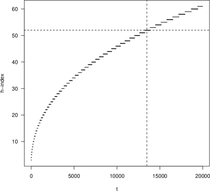
Figure 4: The estimated values of the $h$-index of Hirsch himself based on the Eq. (12) in each time point $t$ ($q=2.5$). The vertical line ($---$) depicts the real value of his $h$-index (equal to 52), while the vertical line depicts the current time point.

6 Conclusions

In this paper we investigated an agent-based model for the bibliometric $h$-index introduced in IonescuChopard . The main contribution included is an exact formula for the number of external citations and self citations for each paper produced by a given author. This result not only completes the work conducted by Ionescu and Chopard, but also gives a perspective for a better insight into the citation process. What is more, we proposed a simplification of the IC model and presented the approximation of the $h$-index based on such an approach. The obtained exact formulas were compared with the results of simulations proposed by Ionescu and Chopard. Interestingly, we may observe a good level of compatibility between them, but mostly for a large number of papers and citations. In this case, however, simulations are more computationally demanding, which makes the usage of the exact formulas more preferable. Also a real data evaluation on an informetric data set was presented.

There are still many issues worth deeper investigation. First of all, due to the analytical formulas one may analyze the theoretical properties of the $h$-$\mathrm{index}$ estimate. Since it has been shown that the $h$-$\mathrm{index}$ is an example of an aggregation operator and its properties can be studied by the means of aggregation theory, it is worth to investigate if such properties are still valid when it comes to the IC model estimate.

Moreover, also the theoretical evaluation of the influence of the considered parameters on the results, which has been done by Ionescu and Chopard only by an empirical study, should be performed. Note that the exact formula for the approximation given by Eq. (17) as well as the comparative study of the proposed approximations of the Hirsch index and the ones already available in the literature opens an interesting future research direction. Also, it is reasonable to perform similar analysis on different data sets, for example representing the data concerning the social network (Facebook, Twitter) users or citation information gathered from different fields of science.

Also, there are a lot of variations of the classical preferential attachment rule, proposed by Barabási and Albert. There is also a rich discussion in the literature on the proper version of those mechanisms for considered problem Golosovsky2013:JStatPhys ; Eom2011:citationdynamisc ; Krapivsky2000:network . Mostly due to the simplicity (and for agreement with original work IonescuChopard ) we chose a classical linear version Jeong ; Newman2011:clustering . The analysis of different forms of preferential attachment rule (as those presented in GolosovskyPRL or Eom2011:citationdynamisc ; Krapivsky2000:network ) is also left for future studies.

Author contributions

Derived the results: BŻS, GS. Analyzed the results: AC, MG. Wrote the paper: BŻS, GS, AC, MG.

References

- (1) A. L. Barabási, R. Albert, Science 286, 509 (1999)
- (2) D. Wang, C. Song, A.-L. Barabási, Science 342, 127 (2013)
- (3) P. Deville, D. Wang, R. Sinatra, C. Song, V. D. Blondel, A.-L. Barabási, Sci. Rep. 4, 2014
- (4) Q. Zhang, N. Perra, B. Goncalves, F. Ciulla, A. Vespignani, Sci. Rep. 3, 2013
- (5) A. Mazloumian, D. Helbing, S. Lozano, R. P. Light, K. Borner, Sci. Rep. 3, 2013
- (6) S. Redner, Eur. Phys. J. B. 4, 131 (1998)
- (7) M. Golosovsky, S. Solomon, J. Stat. Phys. 151, 340 (2013)
- (8) H. Jeong, Z. Néda, A. L. Barabási, Europhys. Lett. 61, 567 (2003)
- (9) Y.-H. Eom, S. Fortunato, PLoS ONE 6, e24926 (2011)
- (10) P. L. Krapivsky, S. Redner, F. Leyvraz, Phys. Rev. Lett. 85, 4629 (2000)
- (11) M. E. J. Newman, Phys. Rev. E 64, 025102 (2001)
- (12) M. Golosovsky and S. Solomon, Phys. Rev. Lett. 109, 098701 (2012)
- (13) D. J. de Solla Price, Science 149, 510 (1965)
- (14) M. Perc, J. R. Soc. Interface 11, 20140378 (2014)
- (15) M. Wang, G. Yu, D. Yu, Phys. A: 387, 4692 (2008)
- (16) M. Wang, G. Yu, D. Yu, Phys. A 388, 4273 (2009)
- (17) G. Ionescu, B. Chopard, Eur. Phys. J. B, 86, 426 (2013)
- (18) J. E. Hirsch, Proc. Natl. Acad. Sci. 102, 16569 (2005)
- (19) K. Fan, Mathematische Zeitschrift 49, 681 (1943)
- (20) M. Gagolewski, R. Mesiar, Inf. Sci. 263, 166 (2014)
- (21) L. Egghe, R. Rousseau, Scientometrics 69, 121 (2006)
- (22) A. F. J. van Raan, Scientometrics 67, 491 (2006)
- (23) Q. L. Burrell, J. Informetrics 1, 16 (2007)
- (24) M. Gagolewski, in Synergies of Soft Computing and Statistics for Intelligent Data Analysis, Springer-Verlag, 2013, edited by R. Kruse et al, p. 359
- (25) M. Gagolewski, J. Informetrics 4, 678 (2011)
- (26) J. E. Iglesias, C. Pecharroman, Scientometrics 73, 303 (2007)
- (27) K. Barcza, A. Telcs, Scientometrics 2, 513, (2009)
- (28) W. Glänzel, Scientometrics 2, 369, (2008)
- (29) W. Glänzel, Scientometrics 1, 187, (2008)