Gain and noise spectral density in an electronic parametric amplifier with added white noise

Abstract

In this paper, we discuss the behavior of a linear classical parametric amplifier (PA) in the presence of white noise and give theoretical estimates of the noise spectral density based on approximate Green’s functions obtained by using averaging techniques. Furthermore, we give analytical estimates for parametric amplification bandwidth of the amplifier and for the noisy precursors to instability. To validate our theory we compare the analytical results with experimental data obtained in an analog circuit. We describe the implementation details and the setup used in the experimental study of the amplifier. Near the threshold to the first parametric instability, and in degenerate-mode amplification, the PA achieved very high gains in a very narrow bandwidth centered on its resonance frequency. In quasi-degenerate mode amplification, we obtained lower values of gain, but with a wider bandwidth that is tunable. The experimental data were accurately described by the predictions of the model. Moreover, we noticed spectral components in the output signal of the amplifier which are due to noise precursors of instability. The position, width, and magnitude of these components are in agreement with the noise spectral density obtained by the theory proposed here.

I Introduction

Parametrically-driven systems and parametric resonance occur in many different physical systems, ranging from the mechanical domain to the electronic, microwave, electromechanic, optomechanic, and quantum domains. In the mechanical domain we have Faraday waves Faraday (1831), inverted pendulum stabilization, stability of boats, balloons, and parachutes Ruby (1996). A comprehensive review of applications in electronics and microwave cavities spanning from the early twentieth century up to 1960 can be found in Ref. Mumford (1960). A few relevant recent applications, in micro and nano systems, include quadrupole ion guides and ion traps Paul (1990), linear ion crystals in linear Paul traps designed as prototype systems for the implementation of quantum computing Raizen et al. (1992); Drewsen et al. (1998); Kielpinski et al. (2002), magnetic resonance force microscopy Dougherty et al. (1996), tapping-mode force microscopy Moreno-Moreno et al. (2006), axially-loaded microelectromechanical systems (MEMS) Requa and Turner (2006); Thomas et al. (2013), torsional MEMS Turner et al. (1998). In the quantum domain we could mention wideband superconducting parametric amplifiers B. H. Eom, P. K. Day, H. G. LeDuc, and Zmuidzinas (2012), squeezing in optomechanical cavities below the zero-point motion Szorkovszky et al. (2011), and parametric amplification in Josephson junctions Castellanos-Beltran et al. (2008) Parametric pumping has had many applications in the field of MEMS, which have been used primarily as accelerometers, for measuring small forces and as ultrasensitive mass detectors since the mid 80’s Binnig et al. (1986). An enhancement to the detection techniques in MEMS was developed by Rugar and Grütter Rugar and Grütter (1991) in the early 90’s that uses mechanical parametric amplification (before transduction) to improve the sensitivity of measurements. This amplification method works by driving the parametrically-driven resonator on the verge of parametric unstable zones.

Here, we study a classical parametric amplifier both in theory and in experiment with analog electronics. We investigate signal and idler responses near the onset of the first parametric instability. We find the experimental results of gain in the signal and idler responses accurately described by the theory. We also investigate the noisy precursors of instability. We provide an analytical expression for the noise spectral density of a parametrically-driven oscillator with added noise. Again, mostly, we have very good agreement between experiment and theoretical predictions. The novelty compared with the work of Wiesenfeld et al. in the 80’s Jeffries and Wiesenfeld (1985); Wiesenfeld (1985) is that we provide a simpler theoretical derivation for the noise spectral density (NSD) based on Green’s functions and the averaging method, in which the contribution of both Floquet multipliers involved are taken into account. Furthermore, we provide an analytical expression for the noise spectral density in terms of the parameters of the system and not in terms of the largest Floquet multiplier, which is left unspecified in their theory. The analytical calculation of the Floquet multipliers can still be a daunting problem to overcome. Another difference, is that below threshold there is no periodic solution, the system is in quiescent mode, a system that was not treated by Wiesenfeld et al.. Because we add noise to a linear parametrically-driven system below threshold, we can fit the NSD when there is no pumping with the NSD of a harmonic oscillator with added noise and thus calibrate the noise level. If we had used Wiesenfeld’s theory the measured noise level would be off by 6dB. In their model there is always a parametric pumping, since the noise is treated as a perturbation around a deterministic limit cycle of a nonlinear dynamical system. Hence, the possibility of calibration of the NSD around a harmonic oscillator limit is not possible, or at least is not clear, in their theory.

The contents of this paper are organized as follows. In Sec. (II) we present our theoretical model, in Sec. (III) we describe our experimental setup, in Sec. (IV) we present and discuss our numerical and experimental results, and in Sec. (V) we draw our conclusions.

II Theory

The block diagram shown in Fig. 1 is an schematic implementation of an electronic circuit of the parametric amplifier. The block with the $\times$ symbol in it represents a multiplier and the box with a $\Sigma$ symbol is a summer. The equation that describes this system is given by

$$LC\frac{d^{2}V_{c}}{ds^{2}}+RC\frac{dV_{c}}{ds}+V_{c}=AV_{p}\cos(4\pi fs)V_{c}+V_{0}\cos(2\pi f_{s}s+\phi_{0}),$$ (1)

where $V_{c}$ is the voltage on the capacitor, $L$ is the inductance, $C$ is the capacitance, $R$ is the resistance, $V_{p}$ is the pump amplitude, $A$ is the amplification factor of the multiplier (with units of $volt^{-1}$), $V_{0}$ is the signal voltage amplitude, $2f$ is the pump frequency, $f_{s}$ is the frequency of the signal, and $\phi_{0}$ is the phase of the signal. We can simplify Eq. (1) with the adimensional time $t=\omega_{0}s$, where $\omega_{0}=1/\sqrt{LC}$, $\gamma=1/Q=R/(\omega_{0}L)$, $F_{p}=AV_{p}$, $F_{0}=V_{0}$. We find

$$\frac{d^{2}x}{dt^{2}}+x=-\gamma\frac{dx}{dt}+F_{p}\cos(2\omega t)x+F_{0}\cos(\omega_{s}t+\phi_{0}),$$ (2)

where $x(t)=V_{c}(t),\;\omega=2\pi f/\omega_{0}$, and $\omega_{s}=2\pi f_{s}/\omega_{0}$.

II.1 The Green’s function of the parametric oscillator

The equation for the Green’s function of the parametrically-driven oscillator described in Eq. (2) obeys

$$\left[\frac{\partial^{2}}{\partial t^{2}}+1+\gamma\frac{\partial}{\partial t}-F_{p}\cos(2\omega t)\right]\;G(t,t^{\prime})=\delta(t-t^{\prime}).$$ (3)

We use the retarded Green’s function which is $G(t,t^{\prime})=0$ for $t<t^{\prime}$. By integrating the above equation near $t=t^{\prime}$, we obtain the initial conditions when $t=t^{\prime}+0^{+}$, which are $G(t,t^{\prime})=0$ and $\frac{\partial}{\partial t}G(t,t^{\prime})=1.0$. Assuming the parameters $\gamma,F_{p}=\mathcal{O}(\epsilon)$, with $0<\epsilon<<1$, we can write the Green’s function in the stable zone of the parametrically-driven oscillator in the first-order averaging approximation Batista (2012) as

$$G(t,t-\tau)\approx G_{0}(\tau)+G_{p}(t,\tau),$$ (4)

with

$$G_{0}(\tau) = \frac{e^{-\gamma\tau/2}}{\omega}\left[\cosh(\kappa\,\tau)\sin(\omega\tau)+\frac{\delta}{\kappa}\sinh(\kappa\,\tau)\cos(\omega\tau)\right],$$

$$G_{p}(t,\tau) = -\frac{\beta}{\omega\kappa}e^{-\gamma\tau/2}\sinh(\kappa\,\tau)\cos(\omega(2t-\tau)).$$

where $\tau=t-t^{\prime}>0$, $\kappa=\sqrt{\beta^{2}-\delta^{2}}$, $\beta=-F_{p}/4\omega$, and $\delta=\Omega/2\omega$, and $\Omega=1-\omega^{2}$.

II.2 The ac-signal response in the parametric oscillator

Here we present the theory on classical linear parametric amplification near the onset of the first instability zone of the parametric amplifier, i.e. we analyze the response of a parametric oscillator to an added input ac signal. In the following, we will use the Green’s function of Eq. (4) to obtain the solution of Eq. (2). This is given by

$$x(t) =\int_{-\infty}^{t}\;G(t,t^{\prime})F_{0}\cos(\omega_{s}t^{\prime}+\phi_{0})\;dt^{\prime},$$ (5)

since we assume the pump and the input signal have been turned on for a long time, any homogeneous solution has already decayed. The signal response is given by

$$\int_{-\infty}^{t}dt^{\prime}\;G_{0}(t-t^{\prime})\cos(\omega_{s}t^{\prime}+\phi_{0})=\mbox{Re}\int_{-\infty}^{t}dt^{\prime}\;G_{0}(t-t^{\prime})e^{-i(\omega_{s}t^{\prime}+\phi_{0})}$$ (6)

$$= \mbox{Re}\left[e^{-i(\omega_{s}t+\phi_{0})}\int_{-\infty}^{t}dt^{\prime}\;G_{0}(t-t^{\prime})e^{i\omega_{s}(t-t^{\prime})}\right]$$

$$= \mbox{Re}\left[e^{-i(\omega_{s}t+\phi_{0})}\int_{0}^{\infty}G_{0}(\tau)e^{i\omega_{s}\tau}\right]=\mbox{Re}\left[e^{-i(\omega_{s}t+\phi_{0})}\tilde{G}_{0}(\omega_{s})\right].$$

In order to obtain

$$\tilde{G}_{0}(\omega_{s}) = \int_{-\infty}^{\infty}e^{i\omega_{s}t}G_{0}(t)dt$$ (7)

$$= \frac{1}{\omega}\int_{0}^{\infty}e^{-\gamma t/2}e^{i\omega_{s}t}\left[\cosh(\kappa\,t)\sin(\omega t)+\frac{\delta}{\kappa}\sinh(\kappa\,t)\cos(\omega t)\right]dt,$$

the following integrals were utilized

$$\int_{0}^{\infty}e^{[-\gamma/2+i(\omega_{s}\pm\omega)]t}\cosh(\kappa t)dt = \frac{\gamma-2i(\omega_{s}+\omega)}{2[\gamma/2-\kappa-i(\omega_{s}\pm\omega)][\gamma/2+\kappa-i(\omega_{s}\pm\omega)]},$$

$$\int_{0}^{\infty}e^{[-\gamma/2+i(\omega_{s}\pm\omega)]t}\sinh(\kappa t)dt = \frac{\kappa}{[\gamma/2-\kappa-i(\omega_{s}\pm\omega)][\gamma/2+\kappa-i(\omega_{s}\pm\omega)]},$$

and we obtained

$$\tilde{G}_{0}(\omega_{s}) \approx \frac{1}{\omega}\left\{\frac{1}{2i}\left[\frac{\gamma-2i(\omega_{s}+\omega)}{2[\gamma/2-\kappa-i(\omega_{s}+\omega)][\gamma/2+\kappa-i(\omega_{s}+\omega)]}\right.\right.$$ (8)

$$- \left.\left.\frac{\gamma-2i(\omega_{s}-\omega)}{2[\gamma/2-\kappa-i(\omega_{s}-\omega)][\gamma/2+\kappa-i(\omega_{s}-\omega)]}\right]\right.$$

$$+ \left.\frac{\delta}{2}\left[\frac{1}{[\gamma/2-\kappa-i(\omega_{s}+\omega)][\gamma/2+\kappa-i(\omega_{s}+\omega)]}\right.\right.$$

$$+ \left.\left.\frac{1}{[\gamma/2-\kappa-i(\omega_{s}-\omega)][\gamma/2+\kappa-i(\omega_{s}-\omega)]}\right]\right\}.$$

Hence, with the help of the appendix calculations, we find the stationary solution of Eq. (2) to be approximately

$$x(t) \approx F_{0}\left\{\mbox{Re}\left[e^{-i(\omega_{s}t+\phi_{0})}\tilde{G}_{0}(\omega_{s})\right]-\frac{\beta}{2\omega}\mbox{Re}\left[\frac{e^{i[(2\omega+\omega_{s})t+\phi_{0}]}}{[\gamma/2-\kappa+i(\omega+\omega_{s})][\gamma/2+\kappa+i(\omega+\omega_{s})]}\right.\right.$$ (9)

$$+ \left.\left.\frac{e^{i[(2\omega-\omega_{s})t-\phi_{0}]}}{[\gamma/2-\kappa+i(\omega-\omega_{s})][\gamma/2+\kappa+i(\omega-\omega_{s})]}\right]\right\}.$$

With $\omega_{s}\approx\omega$ and when the PA is pumped near the onset of the first instability, we find the idler response to be

$$\int_{-\infty}^{t}dt^{\prime}\;G_{p}(t,t^{\prime})\cos(\omega_{s}t^{\prime}+\phi_{0})\approx-\frac{\beta}{2\omega}\mbox{Re}\left\{\frac{e^{i[(2\omega-\omega_{s})t-\phi_{0}]}}{[\gamma/2-\kappa+i(\omega-\omega_{s})][\gamma/2+\kappa+i(\omega-\omega_{s})]}\right\}.$$

We also find that the envelope of the time series $x(t)$ given in Eq. (9) is approximately

$$\left|e^{-i[(\omega-\omega_{s})t-\phi_{0}]}\tilde{G}_{0}^{*}(\omega_{s})-\frac{\beta}{2\omega}\frac{e^{i[(\omega-\omega_{s})t-\phi_{0}]}}{[\gamma/2-\kappa+i(\omega-\omega_{s})][\gamma/2+\kappa+i(\omega-\omega_{s})]}\right|$$ (10)

II.3 Noise spectral density in the parametric oscillator

We will now investigate the effect of noise on the parametrically-driven oscillator Batista (2011). The parametric oscillator equation with added noise is given by

$$\ddot{x}=-x-\gamma\dot{x}+F_{p}\cos(2\omega t)\;x+r(t),$$ (11)

where $r(t)$ is a Gaussian white noise that satisfies the statistical averages $\langle r(t)\rangle=0$ and $\langle r(t)r(t^{\prime})\rangle=2D\delta(t-t^{\prime})$, where $D$ is the noise intensity. We shall now use the same analytical method developed in Refs. Batista (2011); Batista and R. S. N. Moreira (2011) to study the parametrically-driven oscillator with noise as given by Eq. (11).

Using the Green’s function we obtain the solution $x(t)$ of Eq. (11), which is given by

$$x(t) =\int_{-\infty}^{t}dt^{\prime}\;G(t,t^{\prime})r(t^{\prime}),$$ (12)

assuming that the added noise has been turned on for a long time, hence, any homogeneous solution has already faded out.

The Fourier transform of $x(t)$ is given by

$$\tilde{x}(\nu) =\int_{-\infty}^{\infty}e^{i\nu t}x(t)dt=\int_{-\infty}^{\infty}dt^{\prime}r(t^{\prime})\int_{t^{\prime}}^{\infty}dt~{}e^{i\nu t}\left[G_{0}(t-t^{\prime})+G_{p}(t,t^{\prime})\right]$$ (13)

$$=\tilde{r}(\nu)\tilde{G}_{0}(\nu)+\int_{-\infty}^{\infty}dt^{\prime}r(t^{\prime})\int_{t^{\prime}}^{\infty}dt~{}e^{i\nu t}G_{p}(t,t^{\prime})$$

Hence, with the help of the appendix calculations, we find

$$\tilde{x}(\nu)=\tilde{r}(\nu)\tilde{G}_{0}(\nu)-\frac{\beta}{2\omega}\left[\frac{\tilde{r}(\nu+2\omega)}{[\rho_{-}+i(\nu+\omega)][\rho_{+}+i(\nu+\omega)]}+\frac{\tilde{r}(\nu-2\omega)}{[\rho_{-}+i(\nu-\omega)][\rho_{+}+i(\nu-\omega)]}\right],$$ (14)

where $\rho_{\pm}=-\gamma/2\pm\kappa$ are the Floquet exponents Batista (2012) in the first-order averaging approximation. Since the stochastic process of a parametrically-driven oscillator with added noise as defined in Eq. (11) is cyclo-stationary, the correlation function of $x(t)$ is not translationally invariant and the Wiener-Khinchin theorem is not valid. Therefore, one needs to perform a time average over the usual NSD Wiesenfeld (1985). One then finds

$$S_{x}(\nu) =\overline{\int_{-\infty}^{\infty}d\tau e^{-i\nu\tau}\langle x(t+\tau)x(t)\rangle}=\frac{1}{2\pi}\overline{\int_{-\infty}^{\infty}d\nu^{\prime}e^{i(\nu-\nu^{\prime})t}\langle\tilde{x}(-\nu)\tilde{x}(\nu^{\prime})\rangle}$$

$$=\lim_{\Delta\nu\rightarrow 0^{+}}\int^{\nu+\Delta\nu}_{\nu-\Delta\nu}\dfrac{\langle\tilde{x}(-\nu)\tilde{x}(\nu^{\prime})\rangle}{2\pi}\;d\nu^{\prime}.$$ (15)

With the help of the relation $\langle\tilde{r}(\nu)\tilde{r}(\nu^{\prime})\rangle=4\pi D\delta(\nu+\nu^{\prime})$, we find, where $\kappa=\imath\kappa^{\prime\prime}$ is imaginary

$$S_{x}(\nu) \approx 2D\left\{|\tilde{G}_{0}(\nu)|^{2}+\frac{\beta^{2}}{4\omega^{2}}\left[\frac{1}{[\gamma^{2}/4+(\nu+\omega-\kappa^{\prime\prime})^{2}][\gamma^{2}/4+(\nu+\omega+\kappa^{\prime\prime})^{2}]}\right.\right.$$ (16)

$$+ \left.\left.\frac{1}{[\gamma^{2}/4+(\nu-\omega-\kappa^{\prime\prime})^{2}][\gamma^{2}/4+(\nu-\omega+\kappa^{\prime\prime})^{2}]}\right]\right\}.$$

or where $\kappa$ is real (nearer the onset of instability),

$$S_{x}(\nu) \approx 2D\left\{|\tilde{G}_{0}(\nu)|^{2}+\frac{\beta^{2}}{4\omega^{2}}\left[\frac{1}{[(\gamma/2-\kappa)^{2}+(\nu+\omega)^{2}][(\gamma/2+\kappa)^{2}+(\nu+\omega)^{2}]}\right.\right.$$ (17)

$$+ \left.\left.\frac{1}{[(\gamma/2-\kappa)^{2}+(\nu-\omega)^{2}][(\gamma/2+\kappa)^{2}+(\nu-\omega)^{2}]}\right]\right\}.$$

When the pumping is turned off ($F_{p}=0$) in Eq. (14) and we take $\omega=1$, we obtain

$$S_{x}(\nu)\approx\frac{D}{2[\gamma^{2}/4+(\nu-1)^{2}]},$$ (18)

which is a very good approximation of the harmonic oscillator noise spectral density in high-$Q$ oscillators. Near the instability threshold and with $\nu\approx\omega$, we obtain

$$\tilde{G}_{0}(\nu) \approx \frac{1}{4i\omega}\frac{-\gamma+2\imath[\delta+\nu-\omega]}{[\gamma/2-\kappa-i(\nu-\omega)][\gamma/2+\kappa-i(\nu-\omega)]},$$ (19)

and the NSD is given approximately by

$$S_{x}(\nu) \approx 2D\left\{|\tilde{G}_{0}(\nu)|^{2}+\frac{\beta^{2}}{4\omega^{2}[(\gamma/2-\kappa)^{2}+(\nu-\omega)^{2}][(\gamma/2+\kappa)^{2}+(\nu-\omega)^{2}]}\right\}$$

$$\approx D\frac{\gamma^{2}/4+[\delta+\nu-\omega]^{2}+\beta^{2}}{2\omega^{2}[(\gamma/2-\kappa)^{2}+(\nu-\omega)^{2}][(\gamma/2+\kappa)^{2}+(\nu-\omega)^{2}]}$$

$$\approx D\frac{\gamma^{2}/4+(\delta+\nu-\omega)^{2}+\beta^{2}}{4\omega^{2}\gamma\kappa}\dfrac{1}{(\gamma/2-\kappa)^{2}+(\nu-\omega)^{2}},$$ (20)

which is not exactly a Lorenzian curve as predicted by Wiesenfeld et al.

III Apparatus

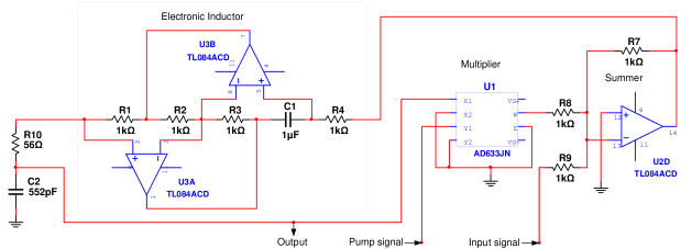
Figure 2: Electronic circuit implementing the parametric amplifier. The 1H electronic inductor is implemented with the aid of operational amplifiers. The IC AD633 represents the multiplier,with a gain of $10V^{-1}$. For simplicity, the output buffer and the power supplies are not shown.

In this section, we describe the electronic circuit conceived to implement a parametric amplifier, which is shown in Fig. 2.

III.1 Analog electronic circuit of the parametric amplifier

The core of the parametric amplifier is shown in Fig. 2 and is comprised of 3 main components: a 4-quadrant analog multiplier (AD633), which has a conversion gain of $1/10V^{-1}$, a (weighted inverting) summer implemented by one operational amplifier (opamp), and an electronic inductor ($1H$) implemented with two opamps (the well-known Antoniou inductor-simulation circuit). Unlike the parametric oscillator circuit of Ref. R. Berthet, A. Petrosyan and Roman (2002), we use a linear capacitor in place of the nonlinear varicap diode, which makes our circuit simpler to analyze. Although nonlinear behavior will eventually appear once the threshold to instability is crossed, we are interested in the operation of the circuit as an amplifier in the linear regime, and not as a nonlinear oscillator.

With the choice of $C_{2}=552$pF, a nominal resonance frequency of $6774Hz$ is obtained. When choosing the capacitor $C_{2}$, care must be taken to avoid lowering the quality factor of the resonator (which is otherwise determined by the quality factor of the inductor along with the value of the resistor $R10$).

The dynamical variable of the circuit is the voltage at the capacitor $C_{2}$, whose readout is buffered before being connected to instruments to avoid current drains during measurements. To avoid outside electromagnetic interference, the PA circuit was enclosed in a metallic box.

III.2 Measurement Setup

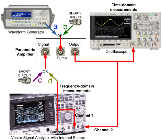
Figure 3: Setup used to characterize the behavior of the parametric amplifier, allowing different operating conditions. With options $b$ and $d$, the PA behaves as a driven harmonic oscillator. With options $a$ and $c$, the PA behaves as a parametric oscillator. With options $a$ and $d$, the PA behaves as a parametric amplifier if the pump is kept below the instability threshold.

The setup used to characterize the behavior of the parametric amplifier is shown in Fig. 3. It is composed of a vector signal analyzer (model $HP89410A$), a waveform generator (model $33210A$), and an oscilloscope (model $MSO-X2024A$). The waveform generator is used to generate the (sinusoidal) pump signal. The vector signal analyzer has an internal source that is used as the signal to be amplified. Moreover, the analyzer has two input channels, which can be configured to evaluate, for example, spectrum ratios. Besides the frequency-domain analysis with the $HP89410A$, we have also observed signals in time-domain with the aid of the oscilloscope.

The setup is flexible enough to enable the experimental characterization of behavior of the Parametric Amplifier under different operating conditions, depending upon whether a short-circuit or a signal source is connected to the inputs of the amplifier. The different measurement configurations are described below.

IV Numerical and experimental results

IV.1 Harmonic oscillator resonant curve

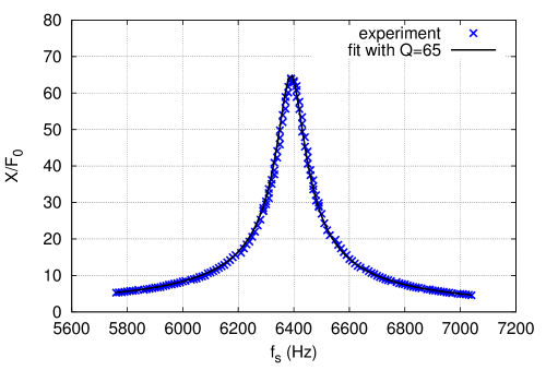
Figure 4: Harmonic oscillator (pump off) resonant curve, obtained using connections $b$ and $d$ in Fig. 3. Here we fit the experimental resonant curve with the theoretic prediction and find a Q of approximately 65 and a resonant frequency of $f_{0}=6400$Hz.

To evaluate the response of the harmonic oscillator, for which $F_{p}=0$ in Eq. (2), the pump input port of the amplifier is short-circuited, while the signal input is fed with a signal source (please refer to Fig. 3, connections $b$ and $d$). We have measured the response (gain) of the harmonic oscillator for a broad range of frequencies. The results are shown in Fig. 4. One can see that the equivalent quality factor Q of the circuit was found to be about 65. This means that if we consider the circuit of Fig. 1, the equivalent series resistance is about $619\Omega$. In addition to the $56\Omega$ shown in Fig. 2, there are additional losses attributed to the electronic inductor, since the quality factor of the capacitor $C_{2}$ was independently measured as about 124. The resonance frequency ($f_{0}=\omega_{0}/(2\pi)$) was found to be around $6400H_{Z}$, a value less than $6\%$ lower than the nominal frequency.

IV.2 Instability boundary

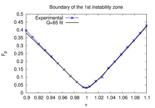
Figure 5: The instability boundary of the amplifier circuit was obtained with the circuit set in parametric oscillator mode, as illustrated in Fig. 3. Above the boundary line, the quiescent state of the circuit ($V_{c}=0$) is unstable and the circuit becomes a nonlinear oscillator, whereas below this line the state $V_{c}=0$ is stable. Very good agreement between experiment and theory was found with the quality factor $Q=65$.

After obtaining the resonance curve of the circuit in harmonic oscillator configuration, we have evaluated the instability boundary of the circuit in parametric oscillator configuration. This configuration is obtained by pumping the amplifier while short-circuiting its signal input. In Fig. 3, this corresponds to connections $a$ and $c$. For each value of pump frequency set, the pump amplitude was slowly increased from a very low initial value until an oscillation of more than $0.5V$ in amplitude was observed at the output of the amplifier. When comparing the experimental data against the numerical data from Eq. (2), we have found that the equivalent Q of the resonator is about 65 (see Fig. 5), a value consistent with the one observed for the harmonic oscillator resonant curve. Moreover, the instability line is centered on the same value of frequency found for the peak of harmonic oscillator resonant curve (about $6400H_{Z}$), which represents half the value of pump frequency for which the lowest pump amplitude is necessary for instability.

Hereafter the parameter values $Q=\gamma^{-}1=65$ and $\omega_{0}\approx 40212$ rad/s will be used in fitting the experimental data of parametric amplification against theoretical predictions.

IV.3 Parametric amplification

Finally, we set the circuit in parametric amplification configuration, by inputing both pump and signal, as described in Fig. 3 with connections $a$ and $d$. In all the results presented below, the input signal amplitude was limited to $2mV$. Owing to the high gains which can be obtained, this value has to be kept small enough to avoid saturation of the amplifier due to limitation of supply voltage bias and intrinsic nonlinearities of the active components of the circuit.

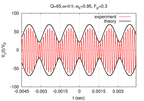
Figure 6: Comparison between a time series from experimental data of $V_{c}(t)$ and corresponding envelope obtained from theory in Eq. (10). The amplification here is set in quasi-degenerate mode with all parameters indicated in the figure.

In Fig. 6, we show a time series obtained from the circuit set with pump amplitude $V_{p}=3V$, pump frequency $1.8f_{0}$ and input signal frequency $f_{s}=0.95f_{0}$, along with the envelope predicted by the Eq. (10) with $F_{p}=0.3$.

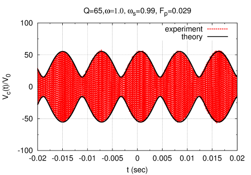
Figure 7: Comparison between time series of experimental data of $V_{c}(t)$ and envelope obtained from theory in Eq. (10). The amplification here is set in degenerate mode with a small detuning between half the pump frequency, $\omega=1$, and the input signal frequency, $\omega_{s}=0.99$.

In Fig. 7, we show a time series obtained from the circuit set with pump amplitude $V_{p}=0.29V$, pump frequency $2f_{0}$ and input signal frequency $f_{s}=0.99f_{0}$, along with the envelope predicted by the Eq. (10) with $F_{p}=0.029$. The best agreement between the experimental time series and the theoretical envelope is obtained under this condition (degenerate-mode amplification). This occurs because the accuracy of the perturbative methods used (averaging and harmonic balance) is higher the smaller the parameter $F_{p}$ is.

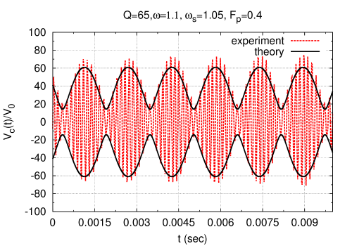
Figure 8: Comparison between a time series from experimental data of $V_{c}(t)$ and envelope obtained from theory in Eq. (10). The amplification here is set in quasi-degenerate mode. All parameters are indicated in the figure.

In Fig. 8, we show a time series obtained from the circuit set with pump amplitude $V_{p}=4V$, pump frequency $2.2f_{0}$ and input signal frequency $f_{s}=1.05f_{0}$, along with the envelope predicted by the Eq. (10) with $F_{p}=0.4$.

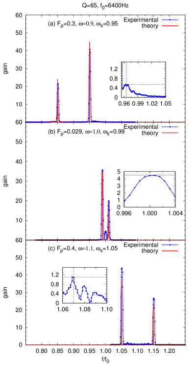
Figure 9: Comparison between experimental data of Fourier transform of $V_{c}(t)/V_{0}$ and numerical Fourier transform of the time series $x(t)/F_{0}$ from Eq. (2). The Fourier transforms refer to the time series presented in previous figures. The position and magnitude of the main peaks (signal and idler) is in agreement with the theoretical prediction of Eq. (9). The insets in frames (a) and (c) zoom in the noise signatures of the experimental Fourier transforms. In frame (b) the middle peak in the experimental data is a noisy precursor of the parametric instability.

In Fig. 9, we show the signal spectrum measured at the output of the amplifier with the aid of the signal analyzer (please refer to Fig. 3). The experimental conditions correspond respectively to those associated with the time series presented in Figs. 6, 7, and 8. The signal analyzer computes the spectrum concurrently to the acquisition of the waveforms by the Oscilloscope. The experimental results are compared against the numerical Fourier transforms of the time series $x(t)$ obtained from numerical integration of Eq. (2). The position and magnitude of the main peaks (signal and idler) is in agreement with the theoretical predictions of Eq. (9). In frame (b), the middle peak in the experimental data is a noisy precursor of the parametric instability, whereas in frames (a) and (c) one hardly notices any effects of noise. To help visualize these effects, the insets in frames (a) and (c) show details of noisy precursors in the experimental data. Further below we will explain why these precursors are more relevant in the degenerate-mode amplification of frame (b), than in cases (a) and (c). In all cases, though, the response of the PA to noise is more pronounced when the amplifier is tuned to the vicinity of the transition line Batista (2011); Batista and R. S. N. Moreira (2011); Batista (2012). Hence, the closer one gets to the transition line, the higher the noisy precursor lines in the spectrum will be. A detailed analysis of the noise spectrum is made in the next subsection. The noisy precursor effect is in qualitative agreement with the observations of Jeffries and Wiesenfeld on the effect of broadband noise on the power spectrum of coherent signals, which was first investigated (theoretically and experimentally) near period-doubling and Hopf bifurcations in a periodically driven $p$-$n$ junction Jeffries and Wiesenfeld (1985); Wiesenfeld (1985) and in the context of parametric amplification in Josephson junctions Bryant et al. (1987).

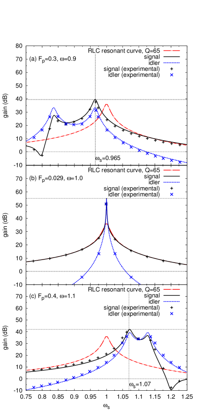
Figure 10: Theoretical signal and idler response gains compared with RLC resonant curve gain. From Eq. (9) the signal gain in dB scale is given by $20\log_{10}(|\tilde{G}_{0}(\omega_{s})|)$, with $\tilde{G}_{0}(\omega_{s})$ given in Eq. (8). Similarly, the idler gain is obtained from Eq. (9). In frames a) and c) the Floquet exponent is complex, what causes the split peaks in the signal and idler responses, whereas in frame b) it is real. As a comparison, we show the gain of the harmonic oscillator response (dot-dashed line).

In Fig. 10 one can see the signal and idler responses of the PA as a function of frequency. Again, one can see that there is a much broader bandwidth of gain in quasi-degenerate mode of amplification, such as in frames (a) and (c), than in degenerate-mode amplification, frame (b). Moreover, the bandwidth of gain, the peak positions, and the gain$\times$bandwidth product can be tuned as well, unlike in the degenerate-mode amplification.

IV.4 Noise spectral density

The spectra of the signal responses can be used to predict where the lines due to noise will turn up in the Fourier transform of the time series $x(t)$, as shown in Fig. 9. Since there is always a small amount of added noise of very broad bandwidth, which comes along with the input ac signal or is intrinsic to the circuit, there will be noise components everywhere in the spectra of Fig. 10. Hence, as our system is linear, the spectral components of noise will be amplified in the same way as the input ac signals are amplified. The strongest case is seen at the peak of degenerate-mode parametric amplification, when $\omega_{s}=1$, where the noise will be amplified roughly by 55dB. The corresponding noise line can be seen in Fig. 9(b). The noise lines in quasi-degenerate-mode parametric amplification are much smaller, since the the peaks in frames 10(a) and (c) have gains of only roughly 39dB and 42dB, respectively. Nonetheless, if one looks in the insets of frames (a) and (c) of Fig. 9, one can see elevations in the noise level exactly at the peaks of the signal response of Fig. 10. The horizontal and vertical dashed lines at the signal peaks of Fig. 10 are reproduced in the insets of Fig. 9 for clarity. One can then compare the magnitudes of the noise line peaks of Fig. 9. The difference in gain at noise line peaks between frame 9(b) and (a) is $20\log_{10}(4.5/0.55)=18.2$dB, whereas between frame (b) and (c) is $20\log_{10}(4.5/1.1)=12.2$dB. On the other hand, the predicted differences in noise peaks based on theory for the signal gain shown in Fig. 10 is 16dB and 13dB, respectively. These results show that our experimental results are consistent with the predictions of our proposed linear theory to within an error of under 2.5dB. We note that the same noise signatures appear in the spectrum when there is no input ac signal, confirming that the noise precursors are a consequence of linear response and a consequence of the signal gain spectra of the PA, such as the ones presented in Fig. 10.

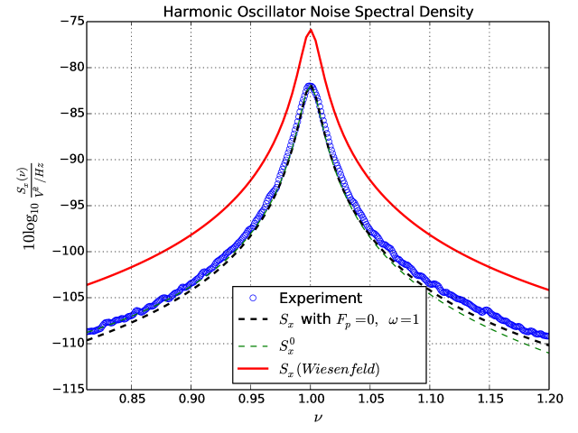
Figure 11: Comparison between theoretical predictions and experimental results for the noise spectral density of a harmonic oscillator. Here $F_{0}=0$. The measuring apparatus depicted in Fig. 3 was setup such that the Signal and the Pump ports were short-circuited (options $b$ and $c$). The results for $S_{x}$ are given by Eq. (17) without parametric pumping and at resonance, whereas $S_{x}^{0}$ is the exact harmonic oscillator spectral density.

In Fig. 11 we show the noise spectral density for our circuit setup in harmonic oscillator mode. Here we fit the data with a noise intensity of $D=3.08\times 10^{-8}$V²/Hz. The source of this noise is intrinsic to the circuit. Here we showed the exact theoretical result for the NSD of a harmonic oscillator process given by $S_{x}^{0}$ alongside the approximate result $S_{x}$ from Eq. (18). In our units $S_{x}$ has dimensions of $V^{2}$, since the time is adimensional. In order to set it in proper units, $S_{x}$ is divided by $\omega_{0}$. Both theoretical predictions yield nearly the same spectrum and account well for the experimental data. On the other hand, the NSD from Eq. (13) of Ref. Jeffries and Wiesenfeld (1985) gives a result that is 6dB higher than the measured noise. Apart from this, their result can be rescaled to be exactly our result from Eq. (18) if one divides their prediction by 4. Here we have a way of measuring the noise level when there is no pumping, whereas in their model, there is no quiescent solution without noise. They developed a perturbative solution due to noise around a limit cycle (an isolated periodic solution) and did not calibrate their solution in the zero pumping limit.

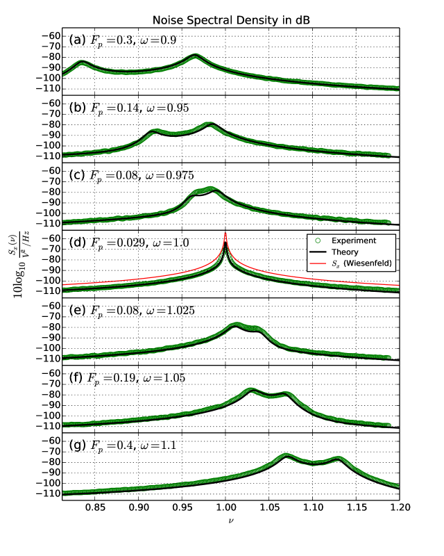
Figure 12: Comparison between theoretical predictions, given by Eq. (17) and experimental results for the noise spectral density of a parametrically-driven oscillator with added white noise. Here $F_{0}=0$. This was achieved in the setup by short circuiting the input signal (option $c$ in Fig. 3). The noise level used here is the same one used in the harmonic oscillator driven by white noise of Fig. 11.

In Fig. 12 one can see the comparison between theoretical predictions, given by Eq. (17) or by Jeffries-Wiesenfeld model, and experimental results for the NSD of a parametrically-driven oscillator with added white noise. Here, the noise level used to fit the data was the same one of the harmonic oscillator configuration. In frames (a-c) and (e-g) the Floquet exponents are still complex, as can be seen in the gap between the noise peaks. These peaks are located symmetrically with respect to $\omega$ and the distance between them is twice the imaginary part of the Floquet exponents. In frame (d) the Floquet exponents are real and, hence, there is no split peak in the noise spectrum. The discrepancy of theory and experiment at the peak of the NSD is certainly due to nonlinear effects not accounted for by our linear model. Again here the Jeffries-Wiesenfeld model is off with a level of noise higher by slightly over 6dB. Note also that the absence of sharp peaks in the spectrum is because we have a quiescent solution and not a periodic orbit solution when there is no noise.

V Conclusion

Here we obtained experimental results on gain and bandwidth of classical parametric amplification that are quantitatively well approximated by a theory based on averaging techniques and on Green’s function theory. Although one can reach extremely high values of gain in degenerate mode parametric amplification, the corresponding bandwidth is very narrow. This is sometimes an undesirable characteristics, since it makes tuning to the signal a difficult task. We have found that the bandwidth of the parametric amplifier can be increased if we set the amplifier in quasi-degenerate-mode amplification, i.e. with detuning ($\Omega\neq 0$). This comes at the expense of the high gain obtained in degenerate-mode amplification. Guided by the model developed here, the optimal amount of gain and bandwidth could be found by carefully tuning the pump frequency and the pump amplitude. Moreover, the bandwidth of gain, the peak positions, and the gain$\times$bandwidth product can be tuned as well, unlike in the degenerate-mode amplification.

Furthermore, we presented a theory for obtaining an approximate analytical expression for the NSD of the parametric oscillator with added noise that accounts for the noisy precursors of instability in the PA. With the information of the signal and idler gain spectra and the input noise level, one could, in principle, determine how the noise features will be manifested in the power spectrum of the output signal of the PA. Although Wiesenfeld et al. Jeffries and Wiesenfeld (1985); Wiesenfeld (1985) developed a general comprehensive model for accounting for the noisy precursors of bifurcations of codimension-1 based on Floquet theory, the model we propose is simpler to apply and has all the theoretical expressions necessary to compare with experimental results. It does not depend on generic unspecified Floquet exponents. It is worthy to mention that the present model describes the simplest nontrivial system to which the generic theory of Wiesenfeld could be applied to, but which was actually overlooked in the literature so far to the authors knowledge. Furthermore, we have results for the noise spectral density that take into account the presence of two Floquet multipliers, and not just one as described in Ref. Wiesenfeld (1985). The existence of two complex Floquet multipliers is characterized by the appearance of two noise peaks in the NSD spectrum, which can be seen in several of our results. This is especially relevant in high $Q$ parametric oscillators, where the stable parameter region in which the Floquet amplifiers are real decreases with increasing $Q$. Hence, it becomes harder to tune into this region, specially, when there is detuning in the pump frequency with respect to the resonance frequency, so one has to account for the contribution from both Floquet exponents. Also, due to this, the noisy precursors spectral curves are not properly Lorenzian anymore.

The predicted gain curves proposed here can be used to determine signal and idler gains, the output noise spectral density, and the figure of noise of the PA (ratio of output and input signal-to-noise ratios of the PA). Furthermore, our PA circuit can be used as a simple and inexpensive experimental platform to test recent theoretical predictions Batista and R. S. N. Moreira (2011); Batista (2011, 2012) on thermal noise squeezing.

Finally, the close proximity of the theoretical predictions and the experimental results obtained here indicates that one could design electronic devices based on PAs that could achieve extremely high gains, have very little noise, and be tunable. Future experimental and theoretical work on the PAs will be performed in analyzing the effects of nonlinearity on the dynamic range of amplification and the phenomenon of noise squeezing. *

Appendix A Idler response calculations

The idler response is given by

$$\int_{-\infty}^{t}dt^{\prime}\;G_{p}(t,t^{\prime})\cos(\omega_{s}t^{\prime}+\phi_{0})=\int_{0}^{\infty}d\tau\;G_{p}(t,t-\tau)\cos(\omega_{s}(t-\tau)+\phi_{0})$$ (21)

$$= -\frac{\beta}{\omega\kappa}\int_{0}^{\infty}d\tau\;e^{-\gamma\tau/2}\sinh(\kappa\,\tau)\cos(\omega(2t-\tau))\cos(\omega_{s}(t-\tau)+\phi_{0})$$

$$= -\frac{\beta}{2\omega\kappa}\int_{0}^{\infty}d\tau\;e^{-\gamma\tau/2}\sinh(\kappa\,\tau)\left[\cos\left((\omega+\omega_{s})(t-\tau)+\omega t+\phi_{0}\right)+\cos\left((\omega-\omega_{s})(t-\tau)+\omega t-\phi_{0}\right)\right]$$

$$= -\frac{\beta}{2\omega\kappa}\mbox{Re}\left\{e^{i\omega t}\int_{0}^{\infty}d\tau\;e^{-\gamma\tau/2}\sinh(\kappa\,\tau)\left[e^{i[(\omega+\omega_{s})(t-\tau)+\phi_{0}]}+e^{i[(\omega-\omega_{s})(t-\tau)-\phi_{0}]}\right]\right\}$$

$$= -\frac{\beta}{2\omega}\mbox{Re}\left\{\frac{e^{i[(2\omega+\omega_{s})t+\phi_{0}]}}{[\gamma/2-\kappa+i(\omega+\omega_{s})][\gamma/2+\kappa+i(\omega+\omega_{s})]}\right.$$

$$+ \left.\frac{e^{i[(2\omega-\omega_{s})t-\phi_{0}]}}{[\gamma/2-\kappa+i(\omega-\omega_{s})][\gamma/2+\kappa+i(\omega-\omega_{s})]}\right\},$$

where we used the following result

$$\int_{0}^{\infty}d\tau\;e^{-[\gamma/2+i(\omega\pm\omega_{s})]\tau}\sinh(\kappa\,\tau) = \frac{1}{2}\left[\frac{1}{\gamma/2-\kappa+i(\omega\pm\omega_{s})}-\frac{1}{\gamma/2+\kappa+i(\omega\pm\omega_{s})}\right]$$ (22)

$$= \frac{\kappa}{[\gamma/2-\kappa+i(\omega\pm\omega_{s})][\gamma/2+\kappa+i(\omega\pm\omega_{s})]}.$$

Appendix B Noise response

We have to solve

$$\int_{t^{\prime}}^{\infty}dt~{}e^{i\nu t}G_{p}(t,t^{\prime})\approx-\frac{\beta}{\kappa\omega}e^{\gamma t^{\prime}/2}\int_{t^{\prime}}^{\infty}dt~{}e^{i\nu t}e^{-\gamma t/2}\sinh(\kappa\,(t-t^{\prime}))\cos(\omega(t+t^{\prime})),$$

$$\int_{t^{\prime}}^{\infty}dt~{}e^{(-\gamma/2+i\nu)t}\sinh(\kappa\,(t-t^{\prime}))\cos(\omega(t+t^{\prime})) =\frac{e^{i\omega t^{\prime}}}{2}\int_{t^{\prime}}^{\infty}dt~{}e^{[-\gamma/2+i(\nu+\omega)]t}\sinh(\kappa\,(t-t^{\prime}))$$

$$+\frac{e^{-i\omega t^{\prime}}}{2}\int_{t^{\prime}}^{\infty}dt~{}e^{[-\gamma/2+i(\nu-\omega)]t}\sinh(\kappa\,(t-t^{\prime}))$$ (23)

$$\int_{t^{\prime}}^{\infty}dt~{}e^{[-\gamma/2+i(\omega+\nu)]t}\sinh(\kappa\,(t-t^{\prime}))=I_{1}+I_{2},$$

where

$$I_{1} = \frac{e^{-\kappa t^{\prime}}}{2}\int_{t^{\prime}}^{\infty}dt~{}e^{[-\gamma/2+i(\nu+\omega)]t}e^{\kappa\,t}=\frac{e^{[-\gamma/2+i(\nu+\omega)]t^{\prime}}}{\gamma-2\kappa-2i(\nu+\omega)}$$

$$I_{2} = -\frac{e^{\kappa t^{\prime}}}{2}\int_{t^{\prime}}^{\infty}dt~{}e^{[-\gamma/2+i(\nu+\omega)]t}e^{-\kappa\,t}=-\frac{e^{[-\gamma/2+i(\nu+\omega)]t^{\prime}}}{\gamma+2\kappa-2i(\nu+\omega)}$$

$$I_{1}+I_{2} = e^{[-\gamma/2+i(\omega+\nu)]t^{\prime}}\left[\frac{1}{\gamma-2\kappa-2i(\omega+\nu)}-\frac{1}{\gamma+2\kappa-2i(\omega+\nu)}\right]$$ (24)

$$= \frac{4\kappa e^{[-\gamma/2+i(\omega+\nu)]t^{\prime}}}{[\gamma-2\kappa-2i(\omega+\nu)][\gamma+2\kappa-2i(\omega+\nu)]}$$

$$\int_{t^{\prime}}^{\infty}dt~{}e^{[-\gamma/2+i(\nu-\omega)]t}\sinh(\kappa\,(t-t^{\prime}))=K_{1}+K_{2},$$

where

$$K_{1} = \frac{e^{-\kappa t^{\prime}}}{2}\int_{t^{\prime}}^{\infty}dt~{}e^{[-\gamma/2+i(\nu-\omega)]t}e^{\kappa\,t}=\frac{e^{[-\gamma/2+i(\nu-\omega)]t^{\prime}}}{\gamma-2\kappa-2i(\nu-\omega)}$$

$$K_{2} = -\frac{e^{\kappa t^{\prime}}}{2}\int_{t^{\prime}}^{\infty}dt~{}e^{[-\gamma/2+i(\nu-\omega)]t}e^{-\kappa\,t}=-\frac{e^{[-\gamma/2+i(\nu-\omega)]t^{\prime}}}{\gamma+2\kappa-2i(\nu-\omega)}$$

$$\int_{t^{\prime}}^{\infty}dt~{}e^{i\nu t}G_{p}(t,t^{\prime}) \approx -\frac{\beta}{\kappa\omega}e^{\gamma t^{\prime}/2}\left[(I_{1}+I_{2})e^{i\omega t^{\prime}}+(K_{1}+K_{2})e^{-i\omega t^{\prime}}\right]/2$$

$$\approx -\frac{\beta}{2\omega}\left[\frac{e^{i(\nu+2\omega)t^{\prime}}}{[\gamma/2-\kappa-i(\nu+\omega)][\gamma/2+\kappa-i(\nu+\omega)]}\right.$$

$$+\left.\frac{e^{i(\nu-2\omega)t^{\prime}}}{[\gamma/2-\kappa-i(\nu-\omega)][\gamma/2+\kappa-i(\nu-\omega)]}\right]$$

$$\int_{-\infty}^{\infty}dt^{\prime}r(t^{\prime})\int_{t^{\prime}}^{\infty}dt~{}e^{i\nu t}G_{p}(t,t^{\prime}) \approx -\frac{\beta}{2\omega}\left[\frac{\tilde{r}(\nu+2\omega)}{[\gamma/2-\kappa-i(\nu+\omega)][\gamma/2+\kappa-i(\nu+\omega)]}\right.$$

$$+\left.\frac{\tilde{r}(\nu-2\omega)}{[\gamma/2-\kappa-i(\nu-\omega)][\gamma/2+\kappa-i(\nu-\omega)]}\right].$$

Figure 1: Schematic block diagram of the proposed analog electronic implementation of the parametric amplifier. The box on the left represents a multiplier with gain $A$ and the box on the right is a non-inverting summer.

References

• Faraday (1831) M. Faraday, Philos. Trans. R. Soc. London 121, 319 (1831).
• Ruby (1996) L. Ruby, Am. J. Phys. 64, 39 (1996).
• Mumford (1960) W. Mumford, Proceedings of the IRE 48, 848 (1960).
• Paul (1990) W. Paul, Rev. of Mod. Phys. 62, 531 (1990).
• Raizen et al. (1992) M. G. Raizen, J. M. Gilligan, J. C. Bergquist, W. M. Itano,  and D. J. Wineland, Phys. Rev. A 45, 6493 (1992).
• Drewsen et al. (1998) M. Drewsen, C. Brodersen, L. Hornekær, J. S. Hangst,  and J. P. Schifffer, Phys. Rev. Lett. 81, 2878 (1998).
• Kielpinski et al. (2002) D. Kielpinski, C. Monroe,  and D. J. Wineland, Nature 417, 709 (2002).
• Dougherty et al. (1996) W. M. Dougherty, K. J. Bruland, J. L. Garbini,  and J. Sidles, Meas. Sci. and Technol. 7, 1733 (1996).
• Moreno-Moreno et al. (2006) M. Moreno-Moreno, A. Raman, J. Gomez-Herrero,  and R. Reifenberger, Appl. Phys. Lett. 88, 193108 (2006).
• Requa and Turner (2006) M. V. Requa and K. L. Turner, Appl. Phys. Lett. 88, 263508 (2006).
• Thomas et al. (2013) O. Thomas, F. Mathieu, W. Mansfield, C. Huang, S. Trolier-McKinstry,  and L. Nicu, Applied Physics Letters 102, 163504 (2013).
• Turner et al. (1998) K. L. Turner, S. A. Miller, P. G. Hartwell, N. C. MacDonald, S. H. Strogatz,  and S. G. Adams, Nature 396, 149 (1998).
• B. H. Eom, P. K. Day, H. G. LeDuc, and Zmuidzinas (2012) B. H. Eom, P. K. Day, H. G. LeDuc, and J. Zmuidzinas, Nature Phys. 8, 623 (2012).
• Szorkovszky et al. (2011) A. Szorkovszky, A. C. Doherty, G. I. Harris,  and W. P. Bowen, Phys. Rev. Lett. 107, 213603 (2011).
• Castellanos-Beltran et al. (2008) M. Castellanos-Beltran, K. Irwin, G. Hilton, L. Vale,  and K. Lehnert, Nature Physics 4, 929 (2008).
• Binnig et al. (1986) G. Binnig, C. F. Quate,  and C. Gerber, Phys. Rev. Lett 56, 930 (1986).
• Rugar and Grütter (1991) D. Rugar and P. Grütter, Phys. Rev. Lett. 67, 699 (1991).
• Jeffries and Wiesenfeld (1985) C. Jeffries and K. Wiesenfeld, Phys. Rev. A 31, 1077 (1985).
• Wiesenfeld (1985) K. Wiesenfeld, J. of Stat. Phys. 38, 1071 (1985).
• Batista (2012) A. A. Batista, Phys. Rev. E 86, 051107 (2012).
• Batista (2011) A. A. Batista, J. of Stat. Mech. (Theory and Experiment) 2011, P02007 (2011).
• Batista and R. S. N. Moreira (2011) A. A. Batista and R. S. N. Moreira, Phys. Rev. E 84, 061121 (2011).
• R. Berthet, A. Petrosyan and Roman (2002) R. Berthet, A. Petrosyan and B. Roman, Am. J. Phys. 70, 744 (2002).
• Bryant et al. (1987) P. Bryant, K. Wiesenfeld,  and B. McNamara, J. Appl. Phys. 62, 2898 (1987).
Refer to caption