A weak gravitational lensing recalibration of the scaling relations linking the gas properties of dark halos to their mass

Abstract

We use weak gravitational lensing to measure mean mass profiles around Locally Brightest Galaxies (LBGs). These are selected from the SDSS/DR7 spectroscopic and photometric catalogues to be brighter than any neighbour projected within 1.0 Mpc and differing in redshift by $<1000$ km/s. Most ($>83\%$) are expected to be the central galaxies of their dark matter halos. Previous stacking analyses have used this LBG sample to measure mean Sunyaev-Zeldovich flux and mean X-ray luminosity as a function of LBG stellar mass. In both cases, a simulation of the formation of the galaxy population was used to estimate effective halo mass for LBGs of given stellar mass, allowing the derivation of scaling relations between the gas properties of halos and their mass. By comparing results from a variety of simulations to our lensing data, we show that this procedure has significant model dependence reflecting: (i) the failure of any given simulation to reproduce observed galaxy abundances exactly; (ii) a dependence on the cosmology underlying the simulation; and (iii) a dependence on the details of how galaxies populate halos. We use our lensing results to recalibrate the scaling relations, eliminating most of this model dependence and explicitly accounting both for residual modelling uncertainties and for observational uncertainties in the lensing results. The resulting scaling relations link the mean gas properties of dark halos to their mass over an unprecedentedly wide range, $10^{12.5}<M_{500}/\mathrm{M_{\odot}}<10^{14.5}$, and should fairly and robustly represent the full halo population.

1 Introduction

Recent measurements of fluctuations in the microwave background have determined the fraction of all matter that is baryonic to high accuracy, $\Omega_{b}/\Omega_{m}=0.158\pm 0.002$, according to Planck Collaboration (2015). At low redshift, the baryon fraction of the richest galaxy clusters is close to this value, with $\sim$85% of the material in the form of X-ray emitting gas and only $\sim$15% in the form of stars (e.g. Allen et al., 2008). In less massive systems, the detected baryon fraction is lower and is dominated, for individual galaxy halos, by the stars in the central galaxy. This contribution maximises at about 4% within the virial radius for galaxies similar in mass to the Milky Way (e.g. Mandelbaum et al., 2006; Wang & Jing, 2010; Guo et al., 2010). In the low redshift universe as a whole, stars account for only a few percent of the expected baryons (Li & White, 2009). Most remain undetected and are thought to be in the intergalactic medium, either photoionised by the metagalactic UV background, or heated, enriched and ejected from galaxy halos by feedback from star formation and/or AGN activity (e.g. Cen & Ostriker, 1999; Ménard et al., 2010; Ménard & Fukugita, 2012; Vogelsberger et al., 2014; Schaye et al., 2015).

Recent stacking results based on the Planck sky maps (Planck Collaboration, 2013) and on the Rosat All Sky Survey (Anderson et al., 2015) have substantially extended the halo mass range over which signals from associated hot gas have been detected. Both studies stacked signals as a function of stellar mass around a sample of Locally Brightest Galaxies (LBGs) taken from the Seventh Data Release of the Sloan Digital Sky Survey (SDSS/DR7 Abazajian et al., 2009). An independent stacking analysis of Planck data by Greco et al. (2015) recently confirmed the original estimates of mean SZ signal as a function of LBG stellar mass. These galaxies are selected to be brighter than any of their neighbours and are predominantly the central galaxies of their dark halos.

The measured Sunyaev-Zeldovich (SZ) and X-ray signals as a function of LBG stellar mass can be converted into scaling relations between halo mass and halo gas properties provided that effective halo mass is known as a function of LBG stellar mass. Both Planck Collaboration (2013) and Anderson et al. (2015) estimated this relation by forward modelling of sample selection and signal measurement using a simulation of galaxy population evolution from Guo et al. (2013). This simulation was tuned to reproduce the observed stellar mass function in the SDSS, so this procedure amounts to an abundance-matching calibration of halo mass. Both scaling relations were found to be unbroken power-laws over the range $10^{12.5}<M_{\mathrm{h}alo}/\mathrm{M_{\odot}}<10^{14.5}$, but whereas the relation for SZ flux was consistent with detection of the cosmic baryon fraction in hot gas at all halo masses (e.g. Planck Collaboration, 2011; Marrone et al., 2012), that for the X-ray flux was substantially steeper than self-similar behaviour would require (e.g. Dai et al., 2007; Rykoff et al., 2008; Vikhlinin et al., 2009; Wang et al., 2014), suggesting that the concentration of baryons within halos must decrease with decreasing halo mass, i.e., the hot gas distribution within lower mass halos is less centrally concentrated than those in massive clusters. Le Brun et al. (2015) showed that when resolution effects in the observations are taken into account, this behaviour can be reproduced by simulations with plausible amounts of AGN feedback.

The results of Planck Collaboration (2013) and Anderson et al. (2015) are intriguing because they seem to indicate the current state of a significant fraction of the baryons which had previously been “missing”. It is, however, a matter of concern that the mass calibration of their scaling relations rests on a specific simulation of the formation and evolution of the galaxy population. The goal of this paper is four-fold: (i) to check the halo mass calibration provided by the model of Guo et al. (2013) by comparing its predictions with weak gravitational lensing measurements for the LBG sample used in the stacking analyses; (ii) to transfer the mass calibration of these scaling relations to one coming directly from the lensing measurements, thus substantially reducing its model dependence; (iii) to evaluate the residual model dependence of this calibration and its origin by comparing results for a large number of different galaxy population simulations; and (iv) to combine the resulting estimate of residual systematic uncertainties with uncertainties coming from noise in the lensing measurements to obtain realistic error bars on the parameters of the recalibrated scaling relations.

The plan of our paper is the following. In Sec. 2, we describe the observational samples and the methods we use to measure differential lensing surface density profiles and two-point autocorrelation functions. Our N-body simulations and the galaxy formation models based on them are introduced in Sec. 3. We present results for differential lensing surface density profiles for SDSS LBGs in Sec. 4 and compare them with predictions from models with varying cosmologies, N-body realisations and physical models for galaxy formation. Galaxy clustering measurements for the SDSS LBGs are compared with various models in Sec. 5. Finally, we recalibrate the scaling relations of Planck Collaboration (2013) and Anderson et al. (2015) in Sec. 6, providing new relations which account consistently for the uncertainties both in effective halo mass and in stacked SZ and X-ray flux for each bin of LBG stellar mass. In a companion paper, Mandelbaum et al. (2015) compare lensing signals for active and passive (e.g. blue and red) subsamples of our LBG sample, finding red LBGs to have significantly more massive halos than blue ones of the same stellar mass, while the same conclusion is reached by Zu & Mandelbaum (2015b) through halo modelling to both lensing and clustering measurements. When quoting observational results, we adopt as our fiducial cosmological model the first-year Planck cosmology (Planck Collaboration, 2014a, with present values of the Hubble constant $H_{0}=67.3\mathrm{\ km\ s^{-1}/Mpc}$, of the matter density $\Omega_{m}=0.315$ and of the cosmological constant $\Omega_{\Lambda}=0.685$). Our simulations assume a variety of other cosmologies as described in Sec. 3. In the following we will define the reduced Hubble parameter h as $\mathrm{h}=H_{0}/100\mathrm{\ km\ s^{-1}/Mpc}$.

2 Observational Samples and Techniques

Figure 1: A scatter plot of our sample of locally brightest galaxies in the redshift – stellar mass plane. Red equidensity contours enclose 10%, 30%, 60% and 90% of the galaxies. To avoid overcrowding only 10% of the sample galaxies are plotted.

2.1 The locally brightest galaxy sample

In order to define a large sample of galaxies that are almost all centrally located and dominant within their dark matter halos, we select locally brightest galaxies (hereafter LBGs) from the New York University Value Added Galaxy Catalogue (Blanton et al., 2005, VAGC), which is based on the seventh data release of the Sloan Digital Sky Survey (Abazajian et al., 2009, SDSS/DR7). This parent catalogue contains 602,251 galaxies with high quality spectra and is flux limited at $r=17.7$ ($r$-band, extinction-corrected Petrosian magnitude).

LBGs are selected to be galaxies that are brighter in $r$ than all other catalogue members projected within 1.0 Mpc and with redshift differing by less than 1000 km/s. The SDSS spectroscopic sample is incomplete due to exclusion effects when placing fibres in crowded fields. To ensure that no candidates have brighter companions without spectroscopy, we have used a photometric redshift catalogue (Cunha et al., 2009, photoz2) based on SDSS/DR7 photometry to look for additional companions missed in the spectroscopic sample. We eliminate any candidate with a companion in this catalogue of equal or brighter $r$-band magnitude and projected within 1.0 Mpc, unless the photometric redshift distribution of the potential companion is inconsistent with the spectroscopic redshift of the candidate.

After this selection 279,343 LBGs remain. Of these, 161,791 have stellar mass greater than $10^{10.8}\mathrm{M_{\odot}}$ (see Sec. 2.2 for details about how the stellar masses are measured). This is the limit to which SZ and X-ray signals have been clearly detected in the stacking analyses of Planck Collaboration (2013) and Anderson et al. (2015), hereafter P13 and A15, respectively. The LBG sample used here differs slightly from that used in these earlier studies, despite being selected according to the same criteria, because in this paper we interpret all data using the cosmology of Planck Collaboration (2014a) whereas the earlier papers adopted that of WMAP7 (Komatsu et al., 2011a). This slightly changes the isolation criterion in projected separation, and also increases the stellar mass assigned to each SDSS galaxy by about 10% (because of the switch from ${\mathrm{h}}=0.704$ to ${\mathrm{h}}=0.673$).

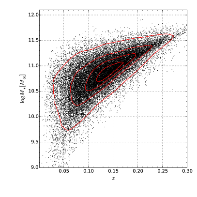
Redshift and colour distributions of the selected LBG sample are shown in Fig. 1 of P13. These are very similar to the corresponding distributions for the parent sample, except that the blue fraction of LBGs is significantly enhanced for objects with stellar mass below that of the Milky Way, shifting the population to slightly higher redshift. Redshift distributions for the specific stellar mass bins used for SZ and X-ray stacking are shown in Fig. 2 of A15, and the numbers, mean distances, estimated mean halo masses and other properties of these subsamples are given in Table 1 of that paper. The mean redshift rises from $z\sim 0.07$ at $M_{*}\sim 10^{10}\mathrm{M_{\odot}}$ to $z\sim 0.3$ at $M_{*}\sim 10^{12}\mathrm{M_{\odot}}$. In Fig. 1, we show a scatter plot of our sample in the redshift – stellar mass plane. Red equidensity contours enclose 10%, 30%, 60% and 90% of the points. Clearly more massive LBGs are biased to higher redshifts as a result of the SDSS flux limit, and at any given stellar mass fewer than half of the objects lie at redshifts where the sample can be considered complete. We will discuss in Sec. 2.5 and Sec. 3.6. how we account for such incompleteness.

P13 and A15 used a galaxy formation simulation (denoted G13–W7^′ below) from Guo et al. (2013) to explore the expected relation of the LBGs to the dark halos in which they reside. Fig. 2 of P13 shows that at every stellar mass, more than 83% of LBGs should be the central galaxies of their halos – of the remaining “satellites” two thirds are included because they are more luminous than the central galaxy of their halo. A scatter plot of main halo mass against stellar mass in Fig. 3 of P13 demonstrates that while a well-defined relation is predicted, it has substantial scatter, a significant high-mass tail due to the remaining satellites, and a noticeable offset between star-forming and passive systems. Histograms of the expected halo mass at each LBG stellar mass are given in Fig. B.1 of P13. These are roughly lognormal with a FWHM of about an order of magnitude. Histograms of the projected offsets of satellite systems from halo centre are shown as a function of stellar mass in Fig. C.2 of P13. These are typically a few hundred kpc.

The distribution of offsets from the true halo centre for satellite LBGs are presented in Fig. C2 of P13, where it is also shown that a more strictly selected sample of LBGs that are locally brightest within $r_{p}=$2Mpc (2000km/s along the line-of-sight) gives almost the same distribution of offsets. With this more strictly selected sample of LBGs, the total number has decreased by 30% for LBGs that are more massive than $\log_{10}M_{\ast}=11$. However, the sample purity of true central galaxies is only slightly increased to about 87% at $\log_{10}M_{\ast}\sim 11$. The selection criteria in P13, A15 and this paper are thus a compromise between sample size and purity. The robustness of the scaling relations against changes in the isolation criteria has been tested in P13 using this more strictly selected sample, showing that the scaling relation is insensitive to the isolation criteria.

2.2 Stellar mass estimation and a reference galaxy sample

The stellar masses used in our analysis were all estimated with the K-correct software of Blanton & Roweis (2007) by fitting stellar population synthesis models to K-corrected, five-band photometry from SDSS assuming a Chabrier (2003) stellar initial mass function. K-correct uses more than 400 spectral templates, of which most correspond to instantaneous burst models from Bruzual & Charlot (2003) based on the Padova1994 isochrones (Fagotto et al., 1994a, b, c).

Moustakas et al. (2013) compared these stellar masses to independently derived values based on 12-band UV to mid-infrared photometry. Comparison has also been made with MPA/JHU stellar masses based on the $H\delta_{A}$ and $D_{n}(4000)$ spectral indices (Kauffmann et al., 2003) in addition to SDSS photometry, as well as with masses from an extension of this method by Salim et al. (2007). Differences between these methods are almost always less than 0.1 dex, with K-correct tending to give systematically slightly higher (lower) values than the other schemes at low (high) stellar mass. A fitting formula quantifying the difference between K-correct and MPA/JHU stellar masses is available in Li & White (2009). Note P13 and A15 used the same K-correct stellar masses to derive the effective halo mass for the SZ/X-ray scaling relations. Any systematic uncertainties beyond the stellar mass, is supposed to be self-consistently removed through the lensing recalibration (see Sec. 6).

In Sec. 5 of this paper we analyse the clustering of LBGs by computing cross-correlations between stellar mass-limited subsamples and a reference galaxy sample. We choose the latter to be all galaxies in the parent spectroscopic sample that are more massive than $10^{10}\mathrm{M_{\odot}}$.

2.3 The source catalogue for lensing

The source galaxy catalogue used for our gravitational lensing study has been described in detail in Reyes et al. (2012), and thus we introduce it only very briefly here. Catalogue construction uses the re-Gaussianization method (Hirata & Seljak, 2003) to correct for the point spread function (PSF) which affects the observed shape of galaxies. Thanks to this PSF correction scheme, Reyes et al. (2012) and Mandelbaum et al. (2012); Mandelbaum et al. (2013) were able to reduce systematic errors significantly compared with previous SDSS source catalogues. More recently, Han et al. (2015) developed an improved maximum-likelihood approach, and with the same source catalogue they measured relations between halo mass and group luminosity with high accuracy. The source galaxy catalogue of Reyes et al. (2012) covers 9243 deg² and fully overlaps the SDSS/DR7 footprint within which our LBGs are selected. It includes all objects with extinction corrected $r$-band model magnitudes brighter than 21.8. Photometric redshifts of the sources have been estimated using the SDSS five-band photometry and the Zurich Extragalactic Bayesian Redshift Analyzer (ZEBRA; Feldmann et al., 2006). The effect of using photometric redshifts in lensing analyses like ours has been quantified by Nakajima et al. (2012).

2.4 Measuring the differential density profile

In this study we follow the method described in Mandelbaum et al. (2005) and Mandelbaum et al. (2006) to calculate mean differential projected density profiles for the total mass distribution stacked around our selected LBGs. We point the reader to Mandelbaum et al. (2005) for full details of this method, and only summarise its main features in this section. Some further details are given in the companion paper, Mandelbaum et al. (2015).

The mean differential surface mass density profile, $\Delta\Sigma(r_{p})$, is defined as the difference between the mean surface density enclosed by projected radius $r_{p}$ (denoted $\bar{\Sigma}(<r_{p})$ and the mean surface density at that radius (denoted $\Sigma(r_{p})$). The quantity $\Delta\Sigma(r_{p})$ can be related to the mean tangential shear, $\gamma_{t}$, and the lensing critical density, $\Sigma_{c}$,

$$\Delta\Sigma=\gamma_{t}\Sigma_{c},$$ (1)

where $\Sigma_{c}$ is defined as

$$\Sigma_{c}=\frac{c^{2}}{4\pi G}\frac{D_{s}}{D_{ls}D_{l}}.$$ (2)

$D_{l}$ and $D_{s}$ refer to the angular diameter distances of lens and source, respectively, and $D_{ls}$ is the angular diameter distance between lens and source. We use physical separations in our analysis rather than comoving separations.

The mean tangential shear can be related to the directly measurable mean tangential ellipticity, $e_{t}$, of source galaxies, the two differing by a factor of twice the shear responsivity, defined as the response of the ensemble averaged ellipticity to a small shear (see Bernstein & Jarvis, 2002). Thus, the mean differential surface mass density profile can be estimated from the mean tangential ellipticity as follows:

$$\Delta\Sigma=\frac{\sum_{i}w_{i}(e_{t}\Sigma_{c})_{i}}{2R\sum_{i}w_{i}},$$ (3)

where $R$ is the shear responsivity. This is essentially a weighted average of $e_{t}\Sigma_{c}$ over the set of stacking centres. The weight, $w_{i}$, involves the inverse square of the total noise, composed of measurement noise, $\sigma_{e_{t},i}$ and shape noise, $\sigma_{SN}$,

$$w_{i}=\frac{\Sigma_{c,i}^{-2}}{\sigma_{e_{t},i}^{2}+\sigma_{SN}^{2}}.$$ (4)

Signals are measured around both real galaxies and random points. The signal around random points should be subtracted from that around real galaxies to remove contributions from systematic shear, though on the scales probed in our analysis such systematics are not significant. Moreover, the signal must be multiplied by a factor of $B(r)=n(r)/n_{\mathrm{rand}}(r)$, which is the the ratio of the number density of sources around real galaxies relative to that around random points. This accounts for dilution of the signal by physically-associated pairs. In the end, we estimate the errors of $\Delta\Sigma(r_{p})$ through jackknife resampling.

For all the lensing measurements in this paper, we follow the convention of this subfield and quote values for $r_{p}$ in physical units; this contrasts with the next subsection and with Section 5 where we follow the convention of the galaxy clustering subfield and quote values for $r_{p}$ in comoving units.

2.5 Clustering measurements

We measure the projected cross-correlation function between LBGs and our reference galaxy sample using the Landy-Szalay estimator (Landy & Szalay, 1993),

$$\xi(r_{p},r_{\pi})=\frac{CD(r_{p},r_{\pi})-CR_{D}(r_{p},r_{\pi})-DR_{C}(r_{p},r_{\pi})}{R_{C}R_{D}(r_{p},r_{\pi})}+1,$$ (5)

where $CD$ is the pair count between central LBGs and the reference sample, $CR_{D}$ is the pair count between LBGs and the random sample corresponding to the reference sample, $DR_{C}$ is the pair count between the reference sample and the random sample corresponding to LBGs, and $R_{C}R_{D}$ is the pair count between the two random samples. $r_{p}$ and $r_{\pi}$ are the projected and the line-of-sight components of the (comoving) separations, respectively.

This estimator thus uses separate random samples corresponding to the LBGs and the reference galaxies. These are constructed to have exactly the same sky coverage, number density, redshift and magnitude distribution as the corresponding real galaxies, but the sky coordinates are randomised within the SDSS footprint.

The SDSS galaxy samples are flux-limited in the $r$-band. As a result, fainter galaxies are only included at lower redshifts (Fig. 1). In order to get volume-limited statistics to allow comparison between samples and with the simulations, we weight individual pairs in the above estimator by $1/\mathrm{min}(V_{\mathrm{max,1,i}},V_{\mathrm{max,1,j}})$, where $V_{\mathrm{max,1,i}}$ and $V_{\mathrm{max,1,j}}$ are the total volumes within which galaxies $i$ and $j$ could be observed, given the SDSS footprint and apparent magnitude limit. This weighting is adopted for all variations of pair counts, i.e. for $CD$, $CR_{D}$, $DR_{C}$ and $R_{C}R_{D}$. It results in volume-weighted statistics provided the mean number per unit volume of correlated pairs with given physical properties (e.g. individual galaxy luminosities and stellar masses and pair separation) varies at most weakly with redshift over the range $0<z<0.15$ which contributes most of the weight to the cross-correlation measurements. We have checked that this is indeed the case for the models we discuss in the next section.

After obtaining $\xi(r_{p},r_{\pi})$, we integrate it to get the projected correlation function,

$$w_{p}(r_{p})=\int\xi(r_{p},r_{\pi})\mathrm{d}r_{\pi},$$ (6)

using a depth of $\pm$ 40 Mpc/h for the line-of-sight integral. This is adequate for projected distances of 10 Mpc or less, as used in our analysis (see Padmanabhan et al., 2009). We estimate error bars for $w_{p}(r_{p})$ through bootstrap resampling 100 subsamples from the full LBG sample. Note, for each subsample the contribution to the counts from individual LBG-reference galaxy pairs can change due to the redistribution of weights assigned to the LBGs. We did not bootstrap companions in the reference sample. As noted above, when compiling pair counts and quoting results for correlation functions we will take $r_{p}$ to refer to a particular comoving projected separation.

3 Galaxy Formation Simulations

Realistic simulations of cosmic structure formation are very valuable when interpreting stacking measurements like those of this paper. To the extent that they represent faithfully both the population of objects used as stacking centres and the environments in which they form, such simulations can characterise the selection effects introduced by observational sample construction and the averaging process inherent in the subsequent stacking. P13 and A15 interpreted their SZ and X-ray stacking analyses of LBGs with a simulation from Guo et al. (2013) that used semi-analytic methods to follow the formation and evolution of galaxies in a high-resolution N-body simulation of a $\Lambda$CDM cosmology. Simulations of this type can be carried out in large volumes and tuned to match the properties of the observed galaxy population quite closely. Here we use this and a number of other simulations to assess how the quantitative interpretation of our results is affected by uncertainties in cosmological parameters and in galaxy modelling assumptions.

3.1 N-body simulations

We use two very large dark-matter-only simulations to represent the distribution of dark matter. These are the Millennium Simulation (Springel et al., 2005, MS) which in its original version adopted cosmological parameters from the first-year data of WMAP (Spergel et al., 2003, WMAP1), and a second simulation (Guo et al., 2013, MS-W7) which is identical to the MS except that the cosmological parameters were taken from the seventh year analysis of WMAP (Komatsu et al., 2011b, WMAP7). The fluctuation phases for the MS-W7 initial conditions are taken from the public, multi-scale, Gaussian, white-noise field (Panphasia) described in Jenkins (2013), and are different from those used for the MS. Table LABEL:tbl:sim provides basic numerical and cosmological parameters for the two simulations. Both follow the same number of particles in a cube of the same side length from redshift 127 to the present day. The dark matter particle mass is slightly larger in the MS-W7 than in the MS.

Table 1: Numerical and cosmological parameters for the simulations used in our analysis

	MS	MS-W7	MS-P′
box size [Mpc/h]	500	500	480
softening [kpc/h]	5	5	4.8
particle mass [$\mathrm{M_{\odot}/h}$]	$8.61\times 10^{8}$	$9.36\times 10^{8}$	$9.62\times 10^{8}$
particle number	$2160^{3}$	$2160^{3}$	$2160^{3}$
$\Omega_{m}$	0.25	0.272	0.315
$\Omega_{\Lambda}$	0.75	0.728	0.685
$\Omega_{b}$	0.045	0.0455	0.0487
$H_{0}[\mathrm{kms^{-1}/Mpc}]$	73.0	70.4	67.3
$n_{s}$	1	0.961	0.96
$\sigma_{8}$	0.9	0.807	0.829
$\sigma_{8}\Omega_{m}^{0.6}$	0.392	0.370	0.415

3.2 Scaling to other cosmologies

In addition to the cosmologies adopted for the original MS and MS-W7, we would like the first-year Planck cosmology (Planck Collaboration, 2014a) to be represented among our galaxy formation simulations. The scaling algorithm developed by Angulo & White (2010) and improved by Angulo & Hilbert (2015) allows the stored output of an N-body simulation to be scaled from the cosmology in which it was originally carried out to a different cosmology. This procedure involves three steps: rescaling the box size, particle mass and velocities, relabelling the output times, and rescaling the amplitudes of individual large-scale fluctuation modes. For this paper we scale the original MS simulation to both the WMAP7 and the Planck cosmologies, in the first case using the parameters of Table 1 in Guo et al. (2013), and in the second the parameters of Fig. 1 of Henriques et al. (2015). We scale the MS to the WMAP7 cosmology to enable direct comparison with MS-W7 for the properties of interest in this paper. Further comparison of the direct and scaled simulations can be found in Guo et al. (2013).

Table LABEL:tbl:output lists available simulation redshifts over the range needed for our analysis. The outputs we use for the original MS and MS-W7 are the same. After scaling the MS to the WMAP7 and Planck cosmologies, the time coordinate is relabelled and the available redshifts are different; for WMAP7, the new $z=0$ corresponds to $z=0.28$ in the original simulation, while for Planck it corresponds to $z=0.12$. The scaled simulation size and particle mass, and the new cosmological parameters are given for the Planck case in Table LABEL:tbl:sim. For the WMAP7 case, the cosmological parameters are the same as for MS-W7 but the scaled box size and particle mass are $521.55\ \mathrm{Mpc/h}$ and $1.0062\times 10^{9}\ \mathrm{M_{\odot}/h}$, respectively. In the next section, we introduce the galaxy formation models used in our analysis, and all models based on a scaled N-body simulation will be indicated by a prime (^′) after their names.

Table 2: Output redshifts used for the MS (columns 1, 3 and 4) and for the MS-W7 (column 2) for the various cosmologies adopted in our analysis

WMAP1	WMAP7	WMAP7-scaled	Planck-scaled
0	0	0	0
0.04	0.04	0.04	0.05
0.09	0.09	0.08	0.08
0.12	0.12	0.12	0.11
0.17	0.17	0.17	0.18
0.24	0.24	0.22	0.22
0.28	0.28	0.27	0.26
0.32	0.32	0.33	0.31

3.3 Galaxy formation models

Table 3: The galaxy formation simulations used in our analysis, showing their different combinations of astophysical modelling (rows) and background cosmology (columns).

	WMAP1	WMAP7	Planck
Guo et al. (2011)	$\mathrm{G11-W1}$	$\mathrm{G11-W7^{\prime}}$	$\mathrm{G11-P^{\prime}}$
Guo et al. (2013)		$\mathrm{G13-W7}$, $\mathrm{G13-W7^{\prime}}$
Henriques et al. (2015)-p	$\mathrm{H15p-W1}$		$\mathrm{H15p-P^{\prime}}$
Henriques et al. (2015)-f			$\mathrm{H15f-P^{\prime}}$

We have used four recent versions of the Munich semi-analytic models to follow the formation and evolution of galaxies in the evolving halo/subhalo population of our four N-body simulations (the original MS and MS-W7, together with the two scaled versions of the MS). Altogether, we consider eight different galaxy formation simulations, which are summarised in Table LABEL:tbl:model. Among these, $\mathrm{G11-W1}$, $\mathrm{G13-W7}$ and $\mathrm{G13-W7^{\prime}}$, and $\mathrm{H15f-P^{\prime}}$ are the models published in Guo et al. (2011), Guo et al. (2013) and Henriques et al. (2015), respectively. For each of these, the uncertain star formation and feedback efficiencies were tuned to produce close fits to SDSS data on the stellar mass functions of low-redshift galaxies, and the resulting model also reproduces observed luminosity and autocorrelation functions quite well. In the case of $\mathrm{H15f-P^{\prime}}$, Henriques et al. (2015) used the abundances and passive fractions of galaxies at $0.4\leq z\leq 3$ as additional constraints on model parameters. Details of how well these models reproduce the observed galaxy population can be found in the original papers.

Our model suite thus includes three different cosmologies, WMAP1, WMAP7 and Planck. The Planck cosmology is available only by using the scaling algorithm introduced above, whereas for the WMAP7 cosmology we have both a direct run and one obtained through scaling the MS. These three cosmologies are indicated by the columns of Table LABEL:tbl:model.

Our model suite includes four different sets of galaxy formation parameters following the recipes of Guo et al. (2011), Guo et al. (2013) and Henriques et al. (2015). These correspond to the rows of Table LABEL:tbl:model. Note that we have two versions of the Henriques et al. (2015) model. H15p is a preliminary version corresponding to that originally submitted and posted on the preprint archive, while H15f is the final version revised and retuned in response to comments from a referee. Compared with the preliminary version, the threshold between major and minor mergers was shifted to produce a better match to the observed morphology distribution of galaxies, and a minor problem with the merger trees was fixed which had led to unphysically rapid growth of the central galaxy of the most massive halo in the simulation.

Thus, $\mathrm{G11-W1}$, $\mathrm{G11-W7^{\prime}}$ and $\mathrm{G11-P^{\prime}}$ have exactly the same galaxy formation physics and parameters, but different cosmologies. $\mathrm{G13-W7}$ and $\mathrm{G13-W7^{\prime}}$ are based on the same cosmology and galaxy formation physics (including all associated parameters) but the former is implemented on MS-W7 and the latter on a scaled version of the MS. $\mathrm{H15p-W1}$ and $\mathrm{H15p-P^{\prime}}$ share the same galaxy formation physics, including all parameters, but are based on WMAP1 and Planck cosmologies respectively. $\mathrm{H15f-P^{\prime}}$ is an updated version of $\mathrm{H15p-P^{\prime}}$, as just noted.

Figure 2: The correction to stellar masses, $\Delta\log M_{\ast}/\mathrm{M_{\odot}}$, needed to bring model stellar mass functions into exact agreement with the observed SDSS stellar mass function. The $x$-axis is the stellar mass after correction, and the correction is defined to be negative when it reduces the stellar masses assigned to galaxies. A horizontal orange dashed line marks zero correction to guide the eye.

Figure 3: Mean halo mass, calculated as $\langle\log M_{200}\rangle$, as a function of stellar mass for LBGs in our eight galaxy formation simulations. The upper panel shows results from the original simulations, while the lower panel shows results after the corrections of Fig. 2 have been used to bring the stellar mass function of each model into exact coincidence with that of the SDSS.

3.4 Corrections to stellar mass through abundance matching

Although the published semi-analytic models of the last section were all tuned to give reasonable matches to the SDSS stellar mass function, a number of other observational constraints such as their luminosity functions, their size, morphology and kinematics distributions, and their clustering were also considered when setting up the physical modelling and determining parameters. In particular, the parameters of the model of Henriques et al. (2015) were adjusted by MCMC sampling to fit not only the low redshift stellar mass function, but also the abundance and passive fractions of galaxies over the redshift range $0<z\leq 3$. Because of these multiple constraints, the quality of the fit to the observed low-redshift SDSS stellar mass function varies between models. This can significantly affect the mass of the halos assigned to galaxies of a specific stellar mass, particularly at high mass.

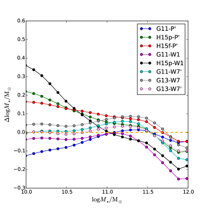
In order to separate differences in model predictions caused purely by deviations from the observed stellar mass function, from differences caused by cosmology or by other aspects of how (sub)halos are populated with galaxies, we use an “abundance matching” method to correct the stellar masses in each model so that it reproduces the SDSS mass function exactly. We preserve the ranking of the model galaxies in stellar mass, but shift them to match the mass function of Li & White (2009). Explicitly, we take the cumulative number density of galaxies at each value of $M_{\ast}$ from SDSS, and find the stellar mass for which the model predicts the same cumulative abundance. The difference between SDSS and model stellar masses at this abundance then gives the necessary correction as a function of stellar mass. Fig. 2 gives the result of this exercise. Notice that over most of the mass range shown the corrections are quite small, demonstrating that the galaxy formation simulations have indeed reproduced the observations quite accurately. In particular, this is true for $\mathrm{G13-W7^{\prime}}$, the model used for comparison in the stacking analyses of P13 and A15.

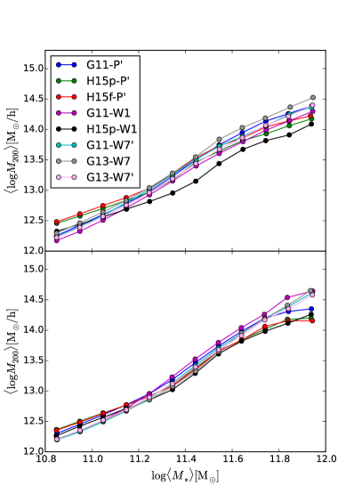
Halo mass – stellar mass relations before and after these corrections to the stellar mass are shown in the top and bottom panels of Fig. 3, respectively. Twelve stellar mass bins have been chosen with a width of 0.1 dex in $\log M_{\ast}$. For each bin, we calculate the mean log halo mass, $\langle\log M_{200}\rangle$ and plot it against the log mean stellar mass, $\log\langle M_{\ast}\rangle$, for all eight galaxy formation simulations. We choose to use $\langle\log M_{200}\rangle$ instead of $\log\langle M_{200}\rangle$ throughout the paper because, as we will see, halo mass distributions at fixed stellar mass are broad and closer to lognormal than to normal. In addition, this definition of mean mass is closer to the effective halo mass implied by SZ, X-ray and lensing observations of stacked BCGs than is $\langle M_{200}\rangle$ (see P13, A15 and Sect. 6 below). On the other hand, we choose to use $\log\langle M_{\ast}\rangle$ because for the narrow stellar mass bins used in this paper the halo mass distribution changes slowly over the bin. We have checked that using $\langle\log M_{\ast}\rangle$, $\log\langle M_{\ast}\rangle$ or the middle bin values gives very similar results.

For the bottom panel of Fig. 3, the stellar mass of each simulated galaxy has been corrected by an amount taken from Fig. 2. The simulations compared here thus have identical stellar mass functions. It is encouraging to see that the scatter between simulations, although not entirely eliminated, is significantly less than in the top panel. The standard deviation among the eight models in the upper panel and for the twelve stellar mass bins are 0.104, 0.090, 0.073, 0.060, 0.068, 0.098, 0.120, 0.111, 0.098, 0.109, 0.130 and 0.131 (from the least to the most massive bin), while for the bottom panel the values become 0.065, 0.065, 0.054, 0.039, 0.036, 0.061, 0.070, 0.056, 0.073, 0.093, 0.136 and 0.198. This demonstrates that much of the scatter between the original models can indeed be ascribed to imperfect matching of the observed stellar mass function. At the most massive end, however, the scatter remains substantial and even becomes bigger, while the models split into two groups after the correction: the Guo et al. group and Henriques et al. group. This indicates that while models with similar physical recipes differ mainly because of the varying degree to which they fit the observed SDSS stellar mass functions, models with differing physical recipes can produce different predictions, even when they are applied to the same N-body simulation and produce the same stellar mass function. This is because they are differently sensitive to the detailed assembly histories of massive halos. Note Fig. 3 only shows the mean halo mass at fixed stellar mass. In Sec. 4, we will show the distribution of $\log M_{200}$, finding that for models with similar mean halo mass at given LBG stellar mass, the shape of the halo mass distribution is very broad and can differ substantially between models.

Figure 4: Left: Differential surface density profiles centred on LBGs in the $\mathrm{G11-P^{\prime}}$ model are compared to our observational results for SDSS (filled circles with error bars). Solid lines are for the original model, while dashed lines include corrections to bring the stellar mass function into exact agreement with SDSS. Lines and symbols are coloured based on the logarithmic range in stellar mass (in units of $\mathrm{M_{\odot}}$) as indicated by the legends. $r_{p}$ is given in physical (not co-moving) units in this and all subsequent plots of this type. The large simulation box size enables us to achieve very small errors for the model (comparable to the symbol size). Note we only show the errors for solid lines. Errors for the dashed lines are of comparable size. Right: The host halo mass distributions for LBGs at $z=0$ within these same stellar mass bins and for the same model, $\mathrm{G11-P^{\prime}}$. Vertical lines mark the characteristic halo mass, $\langle\log M_{200}\rangle$ for each histogram. Black lines correspond to the original model, and red lines to the model after correction to reproduce the SDSS stellar mass function exactly.

3.5 Selecting locally brightest galaxies in the models

We select LBGs in our simulations as in P13 and A15 using criteria patterned closely on those used to select SDSS LBGs (see also Wang & White 2012 and Wang et al. 2014). Specifically, we project the simulation box along its $z$-axis (representing the line-of-sight) and assign each model galaxy a redshift based on its $z$-coordinate and velocity. Isolation criteria in projected separation and redshift difference can then be applied to the simulation in the same way as to the observational data. Such direct projection of the simulation box maximises statistical signal, but fails to represent effects due to the flux limit of the real survey, to the K-corrections needed to obtain rest-frame magnitudes from the observations, to the incompleteness for close pairs caused by fibre exclusion effects, to the complex geometry of the real survey, and to the evolution of the real population across the redshift range surveyed. Wang & White (2012) and Wang et al. (2014) have tested that, for many of these effects, the results obtained by simply projecting the simulation box are unbiased compared to results obtained from a full light-cone mock catalogue. As described below, we combine data from a range of simulation outputs (see Table LABEL:tbl:output) to account consistently for the effects of evolution and of the flux limit of the observational survey.

In the simulations we know whether each selected LBG is truly a central galaxy. As noted in Sect. 2, the fraction of LBGs that are central galaxies (i.e. the purity of the sample) is predicted by $\mathrm{G13-W7^{\prime}}$ to exceed 83% at all stellar masses. The maximum contamination ($\sim 17\%$) by satellites is predicted to occur at stellar masses slightly above $10^{11}\mathrm{M_{\odot}}$. P13 checked those LBGs that are satellites, finding that for $M_{\ast}\geq 10^{11}\mathrm{M_{\odot}}$ about two-thirds are brighter than the true central galaxies of their halos. The remainder are fainter than their centrals, and are considered locally brightest because they are projected more than 1 Mpc from their centrals (60%) or have redshifts differing by more than 1,000 km/s. This high level of purity allows us to consider our LBG sample as a sample of central galaxies with only minor contamination by satellites.

The projected offsets of satellite LBGs from true halo centre are analysed in Appendix C of P13 and are typically a few hundred kpc. It is shown there that a more strictly selected sample of LBGs (selected to be locally brightest within a projected separation of 2 Mpc and a redshift difference of 2000 km/s) has a very similar offset distribution and, despite a 30% reduction in sample size, only a slightly improved level of purity, about 87% for $M_{\ast}\geq 10^{11}\mathrm{M_{\odot}}$.

3.6 Stacked lensing density profiles in the simulations

Our SDSS sample of LBGs is flux-limited in the $r$-band and hence strongly biased towards higher stellar mass (actually higher luminosity) at higher redshift (see Fig. 1). The redshift range spanned is approximately $0<z<0.35$, so that high mass LBGs are seen at a systematically slightly earlier stage of cosmic evolution, thus on a slightly different $M_{\ast}$ – $M_{200}$ relation, than low mass systems. Moreover, the lensing signal measured around each galaxy in a stack is weighted by the inverse square of the (redshift-dependent) lensing critical density, $\Sigma_{c}$ (see Mandelbaum et al. (2006) and Sec. 2.4). To compare our simulations appropriately to our SDSS measurements, we thus need to reproduce the stellar mass – redshift distribution of the observations and to assign the same weights to objects when stacking. Our procedure to achieve this is as follows.

(1) Each SDSS LBG is matched to ten simulated LBGs based on redshift, stellar mass and luminosity. Explicitly, an SDSS LBG is first matched to the simulation output which is closest to its redshift. Ten simulated LBGs are then picked from this output, with stellar mass and $r$-band absolute magnitude differing from the SDSS values by less than 0.02 dex and 0.05 mag, respectively. If fewer than ten simulated galaxies satisfy these requirements, the tolerances are increased iteratively by factors of 1.5 until ten simulated galaxies are matched. In this way, the SDSS and simulation LBG samples end up with identical joint distributions of stellar mass, $r$-band luminosity and redshift.

(2) Each matched LBG in the simulation is assigned the redshift of the corresponding SDSS LBG, and is given a “weight” equal to the mean weight (Eqn. 4) averaged over the background source population of SDSS galaxies at that redshift.

(3) Matched LBGs are grouped by stellar mass in the simulation, after scaling by a factor of $({\mathrm{h_{sim.cosm.}}}/{\mathrm{h_{planck}}})^{2}$. This is to treat the simulation as though we do not know its true cosmology, and so compare it to observation assuming our fiducial Planck cosmology. The differential surface density profiles of dark matter particles around the matched LBGs are calculated as a function of physical (not comoving) projected radius, $r_{p}$, and are averaged using the weights assigned in the previous step.

4 Stacked lensing surface density profiles

4.1 Fit quality for a “good” model

We start by presenting our measurements of differential surface density profiles for stacks of SDSS locally brightest galaxies. We compare these with predictions from $\mathrm{G11-P^{\prime}}$, which turns out to be the simulation that gives the best overall fit to the observational data. $\mathrm{G11-P^{\prime}}$ is also special in that it requires the smallest correction of all our models (see Fig. 2) to bring its high-mass stellar mass function ($\log M_{\ast}/\mathrm{M_{\odot}}>10.7$) into exact agreement with that derived for the SDSS by Li & White (2009). Its behaviour at high mass in the lower panel of Fig. 3 is notable for dropping below that of the other Guo et al. models.

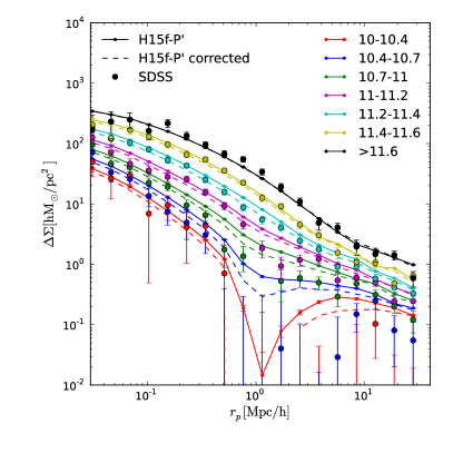
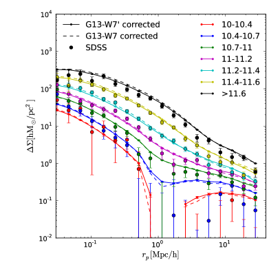
Points with error bars in the left-hand plot of Fig. 4 show observational results from SDSS for LBGs stacked into seven bins of $\log M_{\ast}/\mathrm{M_{\odot}}$ with boundaries as indicated by the legend. Here and in all later similar plots, $\Delta\Sigma$ is given as a function of projected radius, $r_{p}$, in physical (rather than comoving) units. Solid lines are the predictions for $\Delta\Sigma(r_{p})$ for these same LBG stellar mass bins from $\mathrm{G11-P^{\prime}}$. Dashed lines are based on the same model, but after correcting to bring its stellar mass function into exact agreement with SDSS (see Sec. 3.4). Because of the large number of dark matter particles in the simulation and the large number of LBGs stacked, the statistical uncertainties on the model predictions are very small, and are indicated only for the solid lines. For SDSS also the uncertainties are small at most radii in all but the lowest stellar mass bins.

The agreement of $\mathrm{G11-P^{\prime}}$ with the SDSS measurements is very good, both in amplitude and in shape over almost three orders of magnitude in projected radius and 1.5 orders of magnitude in stellar mass. Both theory and observation show a clear transition between a small-scale “one-halo” term, where the signal is dominated by the LBGs’ own halos, and a large-scale “two-halo” term, where the signal is dominated by the correlated environment surrounding the LBG halos. The transition region is distorted by a feature at $\sim 1~{}\mathrm{Mpc}$ induced by our requirement that LBGs should have no brighter companion projected within this radius. The stellar mass corrected and uncorrected cases are very similar at high mass, where the corrections are small; differences are more noticeable in the lowest mass bins. For the 18 data points shown, the $\chi^{2}$ differences between the observed profiles and the uncorrected model are 20.45, 52.40, 14.95, 36.48, 44.79, 48.93 and 54.79 for the most massive to the least massive bin. For the stellar mass corrected model, the corresponding values are 32.74, 44.14, 12.29, 36.10, 54.03, 67.35 and 66.12. While many of these values are formally sufficient to exclude the model, they actually represent remarkably good fits given the small size of many of the formal (bootstrap) error bars and the fact that no model parameters were adjusted to fit these data.

As we will see later through comparison with other simulations, the excellent agreement of $\mathrm{G11-P^{\prime}}$ with SDSS is especially notable for the three most massive bins. The model also agrees reasonably well with the observations for the four lower mass bins, but it seems to have some difficulty reproducing the one-halo/two-halo transition and the 1.0 Mpc/h feature induced by our isolation criterion. The one-halo/two halo transition has often proved difficult to fit accurately with physical or phenomenological models of clustering (see, e.g. Zehavi et al., 2011; van den Bosch et al., 2013; Zu & Mandelbaum, 2015a, for Halo Occupation Distribution fits to galaxy autocorrelations in SDSS). The 1.0 Mpc/h feature is due to the requirement of no brighter companions within 1 Mpc, which translates to a plummeting of the differential surface density profiles at this scale because galaxies trace the underlying mass distribution. This is especially true for low mass LBGs, as our method makes us preferentially select rather isolated systems.

Figure 5: Top Left and Bottom Left: As Fig. 4 but for $\mathrm{G11-W1}$. Top Right and Bottom Right: As Fig. 4 but for $\mathrm{H15f-P^{\prime}}$.

Figure 6: Top Left and Bottom Left: As Fig. 4 but now comparing $\mathrm{G11-W1}$ and $\mathrm{H15p-W1}$ after both have been corrected to reproduce the SDSS stellar mass function. These two models thus have exactly the same stellar mass function and cosmology (WMAP1) and are implemented on the same simulation (the original MS), yet they make substantially different predictions for the lensing profiles and have different halo mass distributions at given stellar mass. Top Right and Bottom Right: As the left-hand plots, but now for $\mathrm{G11-P^{\prime}}$ and $\mathrm{H15f-P^{\prime}}$, two simulations based on the Planck cosmology.

Figure 7: As Fig. 4, but now comparing $\mathrm{G13-W7}$ and $\mathrm{G13-W7^{\prime}}$, two models with the same galaxy formation physics and cosmology (WMAP7), one implemented on a simulation executed with that cosmology (MS-W7) and the other implemented on a scaled version of the MS. Corrections to bring the stellar mass function into exact agreement with SDSS have been included in both cases. Differences here are due to cosmic variance and to inadequacies of the scaling procedure.

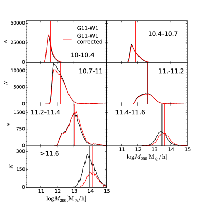
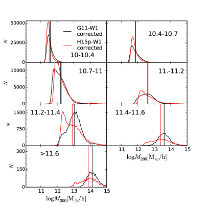
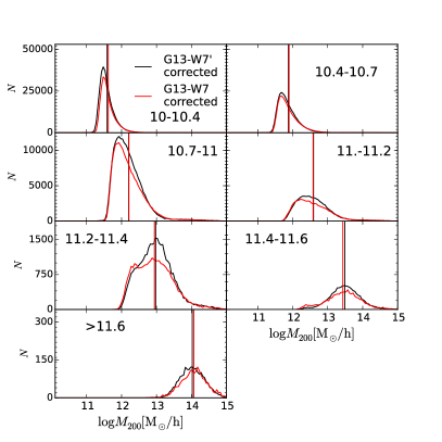
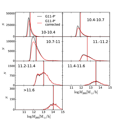
The right-hand plot in Fig. 4 shows histograms of host halo mass for LBGs in our seven stellar mass bins. For simplicity, here and throughout the paper we use LBGs selected in the $z=0$ snapshot to make these plots. For non-central LBGs, the $M_{200}$ values adopted are those of the central galaxies of which they are satellites. Black and red histograms in Fig. 4 refer to the stellar mass uncorrected and stellar mass corrected cases, respectively, as noted in the legend. Vertical lines mark the characteristic halo mass, $\langle\log M_{\mathrm{200}}\rangle$, for each bin. We adopt $\langle\log M_{200}\rangle$ (instead of, for example, $\log\langle M_{200}\rangle$) because the halo mass distributions are broad and roughly lognormal so that $\langle\log M_{200}\rangle$ values are in all cases close to the central values of the distributions. They also turn out to be close to the “effective” halo masses defined by the SZ and X-ray stacking analyses of P13 and A15.

The scatter in halo mass at fixed stellar mass is large and depends both in width and in shape on stellar mass (and, as we will see below, on galaxy formation model). For the four most massive bins, the corrected and uncorrected models give almost the same distribution, explaining why the solid and dashed lines are almost indistinguishable in the left plot. For the three least massive bins, the distributions shift slightly to the right for the mass corrected model, giving higher characteristic halo masses and higher predictions in the left-hand plot. The amplitude differences in the predicted lensing signal agree qualitatively with the shifts in characteristic mass of the halo mass distributions. Despite these small amplitude shifts, both solid and dashed curves agree quite well with SDSS.

4.2 Fit quality for two published Munich models

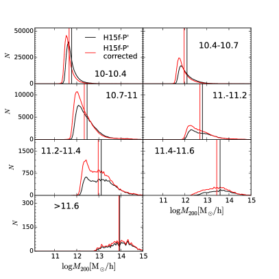
The model analysed in the last section, $\mathrm{G11-P^{\prime}}$, implements the galaxy formation physics and parameters of Guo et al. (2011) on a version of the MS scaled to the Planck cosmology first used in Henriques et al. (2015). As a result, it does not correspond to any previously published galaxy formation simulation. In order to start our exploration of the model-dependence of predicted lensing surface density profiles, we now present results for two published and publicly available simulations, $\mathrm{G11-W1}$, which is based on the WMAP1 cosmology and was published by Guo et al. (2011), and $\mathrm{H15f-P^{\prime}}$, which is based on the Planck cosmology and was published by Henriques et al. (2015). Fig. 5 shows differential lensing surface density profiles and halo mass distributions for these two models in exactly the same format as Fig. 4. Both stellar mass corrected and stellar mass uncorrected results are shown for both models. Note round dots with errors are lensing profiles based on SDSS, which are exactly the same in all relevant plots from Fig. 4 to Fig. 8 and also for Fig. 10. For these figures we always only show errors for solid curves, while errors associated to dashed curves have similar size. In most cases the model predictions have extremely small errors comparable to the symbol size.

The left side of Fig. 5 shows results for $\mathrm{G11-W1}$. As can be seen from Fig. 2, this model requires significant and negative corrections at high mass to bring its stellar mass function into agreement with SDSS, i.e. it overpredicts the abundance of high mass galaxies (see Fig. 7 of Guo et al., 2011). After correction, the predicted surface density profile for the two highest mass bins lies significantly above the observations, showing that the excellent agreement found for the original model is, in fact, a coincidence. For the lower stellar mass bins, the solid and dashed curves are very similar since the required mass corrections are very small in this stellar mass range. For all seven bins, the differences in characteristic halo mass (the shifts between the red and black vertical lines in the lower plot) agree quite well with the shifts in amplitude between solid and dashed lines in the upper plot. This shows that correcting the model stellar masses induces a (logarithmic) shift in the “effective halo mass” (defined as the halo mass which would produce the same signal when all LBGs are assumed to have identical halos) which is very similar to that in the characteristic halo mass $\langle\log M_{200}\rangle$. This implies that the shape of the halo mass distributions at fixed stellar mass is not much affected by the correction.

There is quite good agreement with SDSS for the five lower mass bins, except that magenta curves underpredict the SDSS signal at projected radii of a few hundred kpc. $\chi^{2}$ values for the fit of the uncorrected $\mathrm{G11-W1}$ model to the SDSS data are 18.05, 17.46, 22.85, 49.02, 24.86, 32.48 and 44.18 from most to least massive bin. For the mass-corrected model, the corresponding values are 157.40, 98.22, 14.39, 46.55, 23.26, 35.56 and 47.75. It is clear that, after stellar mass correction, the $\mathrm{G11-W1}$ model fits observation much less well than $\mathrm{G11-P^{\prime}}$, at least for the two highest stellar mass bins.

The right side of Fig. 5 shows similar results for $\mathrm{H15f-P^{\prime}}$. The SDSS signal is clearly underestimated between 200 kpc and 2 Mpc in the most massive bin, and this problem is not affected by the mass correction because this particular model fits the high-mass tail of the SDSS stellar mass function very well (see Fig. 2 of Henriques et al., 2015, note also that the abundance at lower masses is underpredicted, giving rise to the positive corrections seen for this model in Fig. 2). For the five lowest stellar mass bins, significant stellar mass corrections cause both the characteristic halo masses and the shape of the halo mass distributions to shift. As a result, the lensing profile predictions in the upper plot are lowered and come into better agreement with SDSS. The $\chi^{2}$ values are 25.34, 25.64, 69.64, 94.26, 165.07, 96.06 and 78.50 for the mass-uncorrected model and 25.49, 28.66, 18.17, 55.73, 78.25, 57.83 and 58.25 after mass correction (again from most to least massive bin). Once more it is true that the changes in amplitude of the surface density profiles (i.e. the shifts in the effective halo mass for lensing) agree well with the shifts in characteristic halo mass seen in the lower plot.

It is clear that overall $\mathrm{G11-W1}$ and $\mathrm{H15f-P^{\prime}}$ agree less well with SDSS than $\mathrm{G11-P^{\prime}}$, especially for the few most massive bins and after correction to bring agreement with the SDSS stellar mass function. For lower stellar mass, the abundance-matching corrections improve the agreement with observation, at least for these models.

4.3 Models differing only in galaxy formation physics

Figure 8: As Fig. 4, but now comparing three simulations with the same galaxy formation physics and parameters, and implemented on the same N-body simulation (the MS) but with different cosmologies ($\mathrm{G11-P^{\prime}}$, $\mathrm{G11-W1}$ and $\mathrm{G11-W7^{\prime}}$). Corrections to bring the stellar mass function into exact agreement with SDSS have been included for all three models. Differences here are thus due almost entirely to the differing cosmologies.

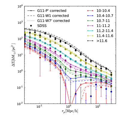
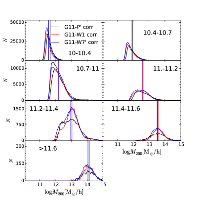
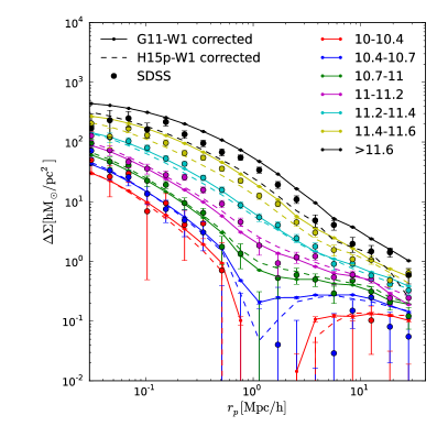
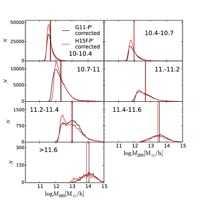
Fig. 6 compares differential surface density profiles and halo mass distributions for two galaxy formation models implemented on the original MS ($\mathrm{G11-W1}$ and $\mathrm{H15p-W1}$ on the left side) and for two implemented on the MS after scaling to the Planck cosmology ($\mathrm{G11-P^{\prime}}$ and $\mathrm{H15f-P^{\prime}}$ on the right side). Thus the models in each pair have the same evolving dark matter distribution but assume different galaxy formation physics. All four models have been corrected to bring their stellar mass distributions into exact agreement with SDSS and so have identical stellar mass functions. Differences within each pair are thus due solely to differences in how galaxies of a given stellar mass are assigned to (sub)halos.

A comparison of $\mathrm{G11-W1}$ and $\mathrm{H15p-W1}$ shows that despite their identical mass distributions and (corrected) stellar mass functions, their surface density profiles differ substantially in the most massive bins, $\mathrm{G11-W1}$ overpredicting the observed signal and $\mathrm{H15p-W1}$ underpredicting it. Corresponding $\chi^{2}$ values are 73.34 and 43.42 for the two most massive bins in $\mathrm{H15p-W1}$ and 157.40 and 98.22 for these same bins in $\mathrm{G11-W1}$. The $\chi^{2}$ values for the five less massive bins of $\mathrm{H15p-W1}$ are 35.44, 35.13, 29.02, 29.64 and 45.66, which are closer to the corresponding $\chi^{2}$ values for $\mathrm{G11-W1}$ (see Sec. 4.2).

These substantial differences highlight the importance of scatter in the stellar mass – halo mass relation. This scatter is not, of course, purely stochastic, but rather a consequence of the scatter in assembly history among halos of given mass, which impacts the properties of central galaxies differently in different galaxy formation models. Scatter effects are particularly important at high mass where the dependence of central galaxy properties on halo mass is weak (e.g. Reyes et al., 2008; Guo et al., 2010; Moster et al., 2010; Wang & Jing, 2010). As a result, central galaxy stellar mass is a relatively poor and model-dependent predictor of halo mass on the scale of rich clusters. More precise mass proxies, perhaps, cluster richness, total luminosity, X-ray or SZ properties (e.g. Rozo et al., 2010; Planck Collaboration, 2014b; Old et al., 2015) will be needed to derive robust and competitive cosmological constraints from the cluster population.

The differences between models are very clear in the halo mass distributions in the lower panels of Fig. 6. In a given stellar mass bin, the distributions can differ substantially in shape, width and characteristic mass, with effects being particularly large in the higher stellar mass bins. $\mathrm{G11-W1}$ predicts less scatter at the massive end of the halo mass – stellar mass relation than $\mathrm{H15p-W1}$. In the lower stellar mass bins, the characteristic halo masses agree better, but the shape and amplitude of the halo mass distributions still differ noticeably.

Similar but less dramatic differences are seen for the two models based on the MS scaled to the Planck cosmology. In the two most massive bins, $\mathrm{G11-P^{\prime}}$ predicts a significantly stronger lensing signal than $\mathrm{H15f-P^{\prime}}$, although the difference is not as big as between $\mathrm{G11-W1}$ and $\mathrm{H15p-W1}$. The $\chi^{2}$ values for the two most massive bins are 25.49 and 28.66 for $\mathrm{H15f-P^{\prime}}$ and 32.74 and 44.14 for $\mathrm{G11-P^{\prime}}$. The behaviour for the five less massive bins parallels that for the WMAP1 models, with $\chi^{2}$ values of 18.17, 55.73, 78.25, 57.82 and 58.25 for $\mathrm{H15f-P^{\prime}}$. Although the characteristic halo masses and differential surface density profiles differ very little between the two models at these stellar masses, the shape and amplitude of the halo mass distributions again differ quite noticeably.

Despite the substantial shape and and scatter variations between these models, the shifts in normalisation of the differential surface density profiles correspond moderately well to the shifts in characteristic halo mass, $\langle\log M_{200}\rangle$ for all stellar mass bins and in both cosmologies. The relative amplitude of the lensing profiles provides an estimate of the change in effective halo mass between two models (see Sec. 6 for details of how we estimate this). The logarithmic shifts from $\mathrm{H15p-W1}$ to $\mathrm{G11-W1}$ are estimated to be 0.469, 0.313, 0.074, -0.076, -0.058, -0.010 and 0.019. from the most to the least massive stellar mass bin. For comparison, the logarithmic differences between the characteristic halo masses indicated by the vertical lines in the bottom left plot are 0.256, 0.216, 0.140, -0.023, -0.052, 0.024 and 0.065. Similarly, the shifts in effective halo mass from $\mathrm{H15f-P^{\prime}}$ to $\mathrm{G11-P^{\prime}}$ estimated from their differential lensing surface density profiles are 0.238, 0.111, 0.027, -0.014, -0.025, 0.001 and 0.028, while the corresponding logarithmic shifts in characteristic mass between their halo mass distributions are 0.150, 0.104, 0.065, -0.012, -0.042, 0.012 and 0.028. The shifts in the effective halo mass for lensing and in $\langle\log M_{200}\rangle$ are similar but certainly not identical. The detailed shape of the halo mass distribution at fixed stellar mass thus affects the ratio of these two masses, rendering it model-dependent.

Table 4: Lensing calibrated characteristic halo masses and their systematic uncertainties as inferred using our full set of galaxy formation simulations. We use each simulation both in its original form and after correction to bring its stellar mass function into exact agreement with the SDSS, resulting in a total of sixteen simulations. For each simulation and each stellar mass bin, we calculate the mean and median values of $\log M_{\mathrm{200}}$. These are then calibrated by shifting logarithmically by the amount needed to bring the simulated differential surface density profile into agreement with the SDSS data (see Sec. 6). Column 1 lists the boundaries of the stellar mass bins; columns 2 and 4 provide lensing calibrated estimates of $\langle\log M_{\mathrm{200}}\rangle$ and $\mathrm{median}(\log M_{\mathrm{200}})$ for our SDSS sample, averaged over all 16 models, while columns 3 and 5 give the rms scatter among estimates for these quantities based on the individual models. $M_{200}$ is in units of $\mathrm{M_{\odot}h}^{-1}$ throughout.

$\log M_{\ast}/\mathrm{M_{\odot}}$	$\langle\langle\log M_{200}\rangle\rangle$	$\sigma(\langle\log M_{200}\rangle)$	$\langle\mathrm{median}(\log M_{200})\rangle$	$\sigma(\mathrm{median}(\log M_{\mathrm{200}}))$
10.-10.4	11.837	0.027	11.778	0.026
10.4-10.7	11.836	0.022	11.743	0.017
10.7-11.	12.234	0.054	12.131	0.051
11.-11.2	12.709	0.043	12.620	0.056
11.2-11.4	13.015	0.047	12.975	0.060
11.4-11.6	13.475	0.064	13.471	0.060
11.6-15.	13.996	0.083	14.000	0.099

4.4 True versus scaled N-body simulations

In this subsection we compare $\mathrm{G13-W7}$ and $\mathrm{G13-W7^{\prime}}$. These two simulations have identical galaxy formation physics, including all parameters, and assume the same cosmology. However, $\mathrm{G13-W7}$ is based on the MS-W7, which was set up and carried out assuming a WMAP7 cosmology, whereas $\mathrm{G13-W7^{\prime}}$ is based on the MS (carried out assuming WMAP1 parameters) after rescaling to a WMAP7 cosmology. We can already see from Fig. 2 that the two models do not produce exactly the same stellar mass function; their mass correction curves differ by about 0.05 dex on all scales (see also Fig. 5 of Guo et al. 2013). Such differences could arise from cosmic variance (since the two simulations have independent initial fluctuation fields), from the (small) differences in time and mass resolution between MS-W7 and the scaled MS, and from inadequate accuracy in the scaling algorithm.

Fig. 7 presents a direct comparison between $\mathrm{G13-W7}$ and $\mathrm{G13-W7^{\prime}}$ in the same format as Fig. 4. For both simulations we have included the corrections needed to bring their stellar mass functions into exact agreement with SDSS. With this source of difference removed, they predict very similar differential surface density profiles. For the few most massive bins, $\mathrm{G13-W7}$ (dashed) is slightly higher than $\mathrm{G13-W7^{\prime}}$ (solid) on small scales. The difference shows up in the $\chi^{2}$ values for the two models: 77.42, 38.36, 13.64, 35.69, 53.71, 47.40 and 50.98 for $\mathrm{G13-W7}$ and 47.02, 21.92, 23.69, 38.77, 51.74, 51.59 and 54.48 for $\mathrm{G13-W7^{\prime}}$. Thus $\mathrm{G13-W7^{\prime}}$ agrees better with SDSS for the two most massive bins, while for the remaining bins the two models have similar $\chi^{2}$ values. We note that $\mathrm{G13-W7^{\prime}}$ is the simulation that was used by P13 and A15 to interpret their SZ and X-ray stacking analyses, and that its agreement with the SDSS lensing data is very good, only slightly worse than that of $\mathrm{G11-P^{\prime}}$, the “best” model of Sect. 4.1

The halo mass functions of the two simulations are compared in Fig. 1 of Guo et al. (2013), where MS-W7 can be seen to have slightly higher halo abundances at $z=0$ than the scaled MS. On the other hand, Fig. 2 shows that at a given stellar mass, $\mathrm{G13-W7}$ predicts slightly lower galaxy abundances than $\mathrm{G13-W7^{\prime}}$. Thus the halo mass – stellar mass relation shifts between the two models, with halos of a given mass forming central galaxies of slightly lower stellar mass in the scaled simulation, perhaps as a consequence of its slightly more widely spaced sequence of output times. Correcting both simulations so that they reproduce the SDSS stellar mass function removes much of this difference.

Halo mass distributions are shown on the right-hand side of Fig. 7. For every stellar mass bin, the two models have similar characteristic halo masses, even though in some cases the shapes of the distributions differ significantly. Here again the logarithmic shifts in characteristic halo mass are similar in size to those in the effective mass corresponding to the lensing profiles. From $\mathrm{G13-W7^{\prime}}$ to $\mathrm{G13-W7}$ the latter shift by -0.063, -0.080, -0.072, -0.053, 0.003, -0.028 and -0.036, while the former shift by -0.040, 0.055, 0.039, 0.012, -0.008, -0.020 and -0.032. The two sets of numbers do not correspond exactly, showing once more a dependence of the ratio of effective to characteristic halo mass on the detailed shape of the halo mass distributions.

4.5 Variations with cosmology

Fig. 8 shows differential surface density profiles and halo mass distributions for three stellar-mass-corrected models with the same galaxy formation physics (including all parameters) but different cosmologies, $\mathrm{G11-P^{\prime}}$, $\mathrm{G11-W1}$ and $\mathrm{G11-W7^{\prime}}$. The differential density profiles for these models are inconsistent with each other, showing that cosmology also has a significant effect on the lensing predictions. However, understanding the source of these differences is not straightforward. Given the extremely small errors of the model predictions (comparable to the symbol size), $\mathrm{G11-W1}$ predicts significantly stronger lensing signals than the other two models for the two highest stellar mass bins. For most of the points over the whole radius range, the significance is a few tens of $\sigma$ with respect to the model errors. Although it is tempting to ascribe this to its higher value of $\sigma_{8}$, $\mathrm{G11-P^{\prime}}$ has a higher value of $\Omega_{m}$ and simple considerations predict the abundance of massive halos at $z=0$ to depend on the combination $\sigma_{8}\Omega_{m}^{0.6}$ which is largest for $\mathrm{G11-P^{\prime}}$ and smallest for $\mathrm{G11-W7^{\prime}}$ (see Table LABEL:tbl:sim). At lower stellar masses, $\mathrm{G11-W1}$ and $\mathrm{G11-W7^{\prime}}$ both predict weaker lensing signals than $\mathrm{G11-P^{\prime}}$. These mass-dependent differences hinder any simple interpretation of the cosmology dependence of the lensing signals.

Despite these complications, we again see a fair correspondence between the differences in effective halo mass (inferred from the relative amplitude of differential surface density profiles) and the differences in characteristic halo mass (found directly from the halo mass distributions). The logarithmic shifts in effective halo mass from $\mathrm{G11-W1}$ to $\mathrm{G11-P^{\prime}}$ are found from their lensing profiles to be -0.156, -0.116, 0.069, 0.135, 0.122, 0.101 and 0.094. The corresponding shifts in characteristic halo mass are -0.081, -0.056, -0.014, 0.074, 0.099, 0.104 and 0.100. From $\mathrm{G11-W7^{\prime}}$ to $\mathrm{G11-P^{\prime}}$, the shifts in effective halo mass are -0.038, 0.029, 0.123, 0.160, 0.165, 0.151 and 0.164, while the shifts in characteristic halo mass are 0.013, 0.045, 0.070, 0.110, 0.106, 0.099 and 0.102. Again, the failure of these sets of numbers to correspond perfectly indicates a model-dependence of the ratio between the effective halo mass for lensing and our characteristic halo mass, $\langle\log M_{200}\rangle$.

4.6 The model dependence of effective halo masses

The differential surface density profiles that we have estimated for the SDSS through gravitational lensing and calculated directly from our galaxy formation simulations are a weighted average of those of the individual galaxies in each stellar mass bin. Similarly, the stacked SZ and X-ray signals estimated from Planck and ROSAT data by P13 and A15 are weighted averages of the signals from individual galaxies, which the modelling relates to halo mass through power-law scaling relations. In all three cases, the stacked signal is very similar to that which would be found if all galaxies had halos of one particular mass, the effective halo mass for that stellar mass bin. The effective halo masses will not be the same in the three cases, however, because of differing weights and differing sensitivity of the observed signal to redshift and halo mass.

If the distribution of halo masses at given stellar mass were always the same shape, for example, lognormal with known width, then the ratios of the effective halo masses to each other and to other characteristic masses such as $\langle M_{200}\rangle$ or $\mathrm{median}(M_{200})$ would always be the same. The direct measurement of any one of these quantities could then be used to calibrate the others. We have seen in previous sections, however, that this is not the case; the shape of the halo mass distribution varies between stellar mass bins and from model to model. This introduces model-dependence into any gravitational lensing based recalibration of the scaling relations linking the SZ and X-ray properties of halos to their mass, a primary goal of this paper. In this subsection we use our suite of galaxy formation simulations to estimate the level of uncertainty resulting from this model-dependence.

In their Table B.1, P13 give SZ effective halo masses together with mean and median values of $M_{200}$ for each stellar mass bin used in their SZ stacking analysis. A15 give X-ray effective halo masses for these same bins in their Table A.1. In both cases, the effective halo masses are estimated using $\mathrm{G13-W7^{\prime}}$ and are much closer to $\mathrm{median}(M_{200})$ than to $\langle M_{200}\rangle$ in each bin. Since we do not wish to repeat the detailed modelling of the SZ or X-ray analyses in this paper, we will assume that the model dependence of the ratio of SZ (or X-ray) effective mass to gravitational lensing effective mass is similar to that of the ratio of $\mathrm{median}(M_{200})$ to gravitational lensing effective mass. The rms scatter in (the logarithm of) this ratio over our set of galaxy formation simulations then provides an estimate of the systematic uncertainty induced by model-dependence when recalibrating the scaling relations of P13 and A15 based on a single simulation, $\mathrm{G13-W7^{\prime}}$. Note that the accuracy of this estimate is not explicitly tested in our analysis. It can only be tested in detail by running the full observational modelling analysis of P13 and A15 on all the other models, which is not possible within the author collaboration of this paper.

In this paper, we consider eight different galaxy formation simulations (see Table LABEL:tbl:model), for each of which we create mock SDSS samples using both the stellar masses originally produced by the simulations and stellar masses corrected so that the simulated stellar mass function matches the SDSS function exactly. Thus, for each of our seven stellar mass bins we end up with 16 different halo mass distributions with corresponding lensing signal predictions. For each case and each bin, we find the shift in halo mass, $\Delta\log M_{200}$, needed to bring the predicted lensing signal into agreement with our SDSS measurement (see Section 6 for details) and we apply this shift to $\mathrm{median}(\log M_{200})$ and $\langle\log M_{200}\rangle$. If the halo mass distributions predicted for the bin by the 16 different models were all the same shape, the 16 values obtained for each characteristic mass would coincide. This is not the case, showing that the ratio of lensing effective mass to characteristic mass is varying from model to model.

Table LABEL:tbl:halomass gives the results of this exercise. For each stellar mass bin, column 2 gives the mean over our 16 simulations of the recalibrated value of $\langle\log M_{200}\rangle$, while column 3 shows the rms scatter among these values. Columns 4 and 5 are similar but for the recalibrated values of $\mathrm{median}(\log M_{200})$. These means are thus our best lensing-based estimates of these particular characteristic halo masses for real SDSS galaxies. The scatter values give estimates of the systematic uncertainty in these means due to their model-dependence. For both quantities the model-dependence is quite small (less than about 0.1 dex) but is an increasing function of stellar mass, reflecting the fact that central galaxy stellar mass becomes a poorer proxy for halo mass in more massive systems. As remarked above, we will later adopt the scatter values given here as estimates of the systematic uncertainty due to model-dependence when using our gravitational lensing observations to recalibrate SZ and X-ray scaling relations for our LBGs.

5 Galaxy Clustering

Figure 9: Projected cross correlation, $w_{p}(r_{p})$, between LBGs and a reference galaxy sample with $\log M_{\ast}/\mathrm{M_{\odot}}>10$. Solid and dashed lines are for $\mathrm{G11-P^{\prime}}$ and $\mathrm{H15f-P^{\prime}}$, respectively. We only show errors for solid lines. These errors are comparable to the symbol size. In both cases stellar masses have been corrected to bring the model stellar mass functions into exact agreement with SDSS. Solid dots with error bars are measurements of $w_{p}(r_{p})$ for real galaxies based on SDSS (see Sect. 2.5). Lensing profiles and halo mass distributions for these two models can be found on the right-hand side of Fig. 6. Note that in this plot $r_{p}$ denotes comoving (rather than physical) separation.

In previous subsections we have compared our SDSS measurements of differential surface density profiles around LBGs to predictions from a range of galaxy formation simulations, finding the latter to be significantly affected by the assumed galaxy formation physics and by the underlying cosmology, even after the model stellar mass functions have been corrected to bring them into exact agreement with SDSS. Such effects are particularly important for massive objects and reflect the considerable (and model-dependent) scatter in the stellar mass – halo mass relation. In this subsection we consider clustering of other galaxies around our LBGs and assess whether this can provide additional information to help choose between models.

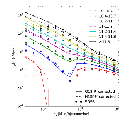
We measure the projected cross-correlation, $w_{p}(r_{p})$, between LBGs and a reference sample, chosen to be all galaxies more massive than $10^{10}\mathrm{M_{\odot}}$ in the SDSS, and also in the simulations. Cross-correlation with a dense reference sample enables us to get better signal than for an autocorrelation, and the low mass threshold reduces the strength of the feature introduced by our isolation criterion. For SDSS, the correlation is measured as outlined in Sec. 2.5. The weighting results in a relatively low effective redshift for the measured signal, with 50% coming from $z<0.08$ and 90% from $z<0.15$ even for our highest LBG stellar mass bin. This reduces evolutionary effects on the signal at the price of increasing the cosmic variance in the measurement. Corresponding cross-correlation functions for the simulations can be measured directly by counting reference galaxies around LBGs in a projection of the $z=0$ snapshot. Note that, in order to be consistent with convention in this subfield, we use $r_{p}$ to denote comoving (rather than physical) separation in this subsection.

In Fig. 9 we compare our SDSS clustering measurement with predictions from two representative models, $\mathrm{G11-P^{\prime}}$ (solid) and $\mathrm{H15f-P^{\prime}}$ (dashed), both with stellar masses corrected to bring their stellar mass function into agreement with that in the SDSS. The lensing signal predicted by these same models is compared with our SDSS results in the upper right panel of Fig. 6. The relative behaviour of the two models is very similar for the two measurements. $\mathrm{G11-P^{\prime}}$ predicts significantly stronger signals than $\mathrm{H15f-P^{\prime}}$ on all scales for the two highest stellar mass bins, given the extremely small errors of the model predictions. Note we only show errors for the solid lines and these errors are mostly comparable to the symbol size. At lower stellar mass their signals are very similar, both for clustering and for lensing. The large-scale clustering amplitudes ($r_{p}\geq 2$ Mpc/h) measure the biasing of LBGs relative to reference galaxies and hence are primarily sensitive to their halo mass, which is measured directly on smaller scales by the one-halo lensing signal. Fig. 6 shows that $\mathrm{G11-P^{\prime}}$ predicts effective halo masses for the two highest stellar mass bins which are slightly above those observed, while those for $\mathrm{H15f-P^{\prime}}$ are clearly too low. The large-scale clustering amplitudes of the two models in Fig. 9 mirror this behaviour relative to the observations as expected. For lower LBG stellar masses, both models fit the observed one-halo lensing and large-scale clustering signals quite well, with the remaining differences probably within the cosmic variance uncertainties of the clustering measurements.

On smaller scales and for intermediate LBG stellar masses ($10.7<\log M_{\ast}/\mathrm{M_{\odot}}<11.4$) the observed clustering signal in SDSS is significantly larger than in either model, indicating that the number of satellites with $\log M_{\ast}/\mathrm{M_{\odot}}>10.0$ is significantly underestimated (although, curiously, not around more or less massive LBGs). We have explicitly checked all the other models, and found such small scale excess persists across cosmologies. This is unexpected, both because Fig. 6 indicates that the models reproduce the mass distribution around these LBGs quite accurately on these same scales, and because Wang & White (2012) found that the count of satellites more massive than $\log M_{\ast}/\mathrm{M_{\odot}}=10.0$ projected within 300 kpc of a large sample of bright isolated galaxies with $10.8<\log M_{\ast}/\mathrm{M_{\odot}}<11.4$ is reproduced quite precisely by $\mathrm{G11-W1}$ (see their Fig. 6). We have not isolated the origin of this discrepancy, which may in part reflect the underestimation of cosmic variance uncertainties by our bootstrap error estimation procedure, but it appears unlikely to affect the main topics of this paper. Note the apparent turnover on very small scales and especially for the few most massive bins is due to the effect that two fibres cannot be assigned closer than 55$\arcsec$.

The two models considered in this section are based on the same simulation, assume the same (Planck) cosmology, and have identical stellar mass functions. They, nevertheless, predict significantly different lensing signals for the most massive LBGs because of differing amounts of scatter in their stellar mass – halo mass relations. The main motivation for the present analysis of clustering was the hope that it would provide an independent observational indication of which model is more realistic. To the extent that it provides a significantly better fit to SDSS measurements for both kinds of data in both the one-halo and the two-halo regime of the two most massive bins, $\mathrm{G11-P^{\prime}}$ appears to be a higher fidelity representation of the real stellar mass – halo mass relation (including scatter) than $\mathrm{H15f-P^{\prime}}$.

Figure 10: Left: As Fig. 4, but now comparing our SDSS lensing measurements (dots and triangles with errors) to the predictions of $\mathrm{G13-W7^{\prime}}$, the model used by P13 and A15. Dashed curves give predictions for the original model, while solid curves are shifted upwards and to the right (or down and to the left) by $(\Delta\log M_{200})/3$, the (potentially negative) amount needed to bring them into optimal agreement with the SDSS data in the one-halo regime, $r_{p}<4R_{200}$ (indicated by a short vertical bar on each curve). Upper triangles are shown in a lighter colour and are not used when fitting because of concerns that they may be affected by light from the LBG. To be consistent with P13 and A15, each LBG in the SDSS was matched in stellar mass alone to LBGs in the $z=0$ output of the simulation when making this plot. Right: Recalibration shifts in $\log M_{200}$ are shown as filled symbols with error bars indicating: (a) statistical uncertainties in the shifts resulting from the error bars on the SDSS lensing measurements; and (b) systematic uncertainties (taken from Table LABEL:tbl:halomass) in the conversion from effective lensing mass to $\langle\log M_{200}\rangle$. The shorter error bar reflects (a) alone, whereas the longer includes (a) and (b) added in quadrature. The pink shaded region interpolates linearly both in the recalibration shift and in its uncertainty.

6 Lensing calibration of SZ and X-ray scaling relations

Figure 11: The SZ $Y_{500}$-$M_{500}$ relation (top left) and X-ray $L_{\mathrm{total}}$-$M_{500}$ relation (top right). Black dots with vertical error bars are the original relations given in P13 and A15. Red dots with both vertical and horizontal error bars are the same measurements after recalibrating the effective halo masses using our lensing measurements. The black and red dashed lines are best-fit power-law scaling relations for the original and the recalibrated data, respectively. Triangles along the red dashed lines indicate the maximum likelihood effective halo masses associated with each stellar mass bin. The bolometric correction, $C^{-1}_{\mathrm{bolo}}$, is included for the X-ray model. This varies between bins, so the model is not strictly a straight line. At each halo mass, the pink shaded regions enclose 68% of the scaling relations proposed by our MCMC chains. The bottom panels show the best-fit parameters from these chains as symbols surrounded by contours indicating their 1- and 2-$\sigma$ confidence regions. Black and red again indicate the original and recalibrated cases, respectively. The confidence regions are larger after recalibration because both systematic modelling uncertainties and random noise in the effective halo mass estimates are now consistently included.

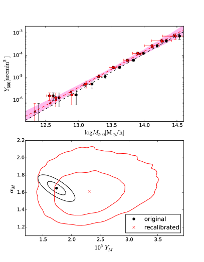
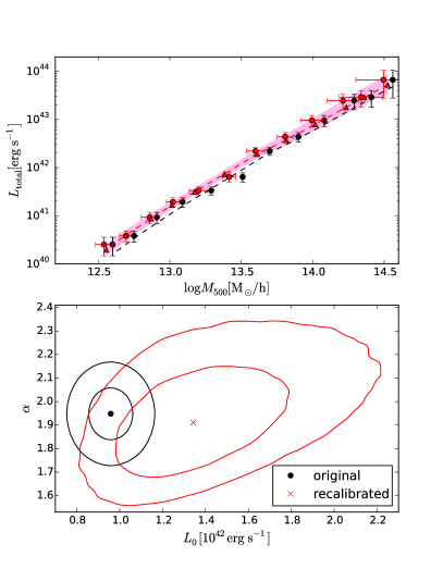
P13 and A15 stacked the Planck and ROSAT sky maps around the LBG sample analysed in this paper in order to measure mean Sunyaev-Zeldovich signals and mean X-ray luminosities as functions of stellar mass. The large sample size resulted in detections to substantially lower masses and with higher precision than had been possible in earlier work. In both papers, $\mathrm{G13-W7^{\prime}}$ was combined with simple assumptions about halo gas profiles and power-law relations between halo mass and observable signal to carry out detailed forward modelling of the stacking and detection procedures. This allowed estimation both of effective halo mass as a function of LBG stellar mass, and of the parameters of the scaling relation between observable and halo mass. Since $\mathrm{G13-W7^{\prime}}$ was originally tuned to reproduce the stellar mass function of the SDSS, this procedure was effectively an abundance-matching calibration of the halo mass–stellar mass relation which, as we have seen in earlier sections, is model-dependent because of: (i) residual mismatch between model and observed stellar mass functions; (ii) uncertainties in the cosmological parameters; and (iii) the model-dependence of the detailed shape of the halo mass distribution at fixed LBG stellar mass (including effects due to varying satellite fractions and offsets).

The goal of the current section is to remove most of this model-dependence by recalibrating the scaling relations of P13 and A15 using our gravitational lensing measurements. The new calibrations will be model-dependent only to the extent that the ratio of the effective halo mass for gravitational lensing to that for SZ (or X-ray) stacking varies between models. Since all three effective masses correspond to rather similar moments of the halo mass distribution, this dependence is quite weak, and we include an estimate of the associated uncertainty in the analysis leading to our final recalibrated scaling relations. When estimating halo masses, P13 and A15 matched the observed LBGs to simulated LBGs of the same stellar mass in the $z=0$ output of $\mathrm{G13-W7^{\prime}}$. For consistency, we will match in the same way in this section, rather than matching in stellar mass, luminosity and redshift, as in earlier sections.

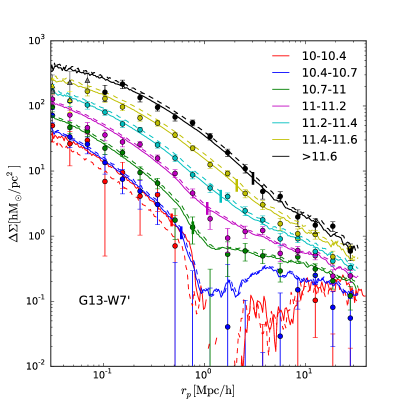
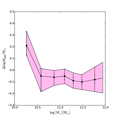
In the left panel of Fig. 10 we compare our SDSS measurements of differential lensing surface density profiles with the predictions of $\mathrm{G13-W7^{\prime}}$. Dashed curves are for the original model, as used by P13 and A15. These are close to the observations, suggesting that the model already represents the halos of SDSS galaxies well, and that the shifts needed to recalibrate to the lensing data will be small. For each stellar mass bin, we estimate the shift (and its uncertainty) by assuming that the halos of all model LBGs change mass by $\Delta\log M_{200}$ without changing concentration. In the one-halo regime, the differential density profiles then shift upwards by $\frac{1}{3}\Delta\log M_{200}$ and to the right by the same amount. We find the best shift and its uncertainty by calculating $\chi^{2}$ values for the model curves with respect to the SDSS data at $r_{p}<4R_{200}$, the region over which Hayashi & White (2008) found the lensing profiles of central galaxies to be well described by the one-halo term. For the three most massive stellar mass bins, we exclude the innermost three, two or one SDSS data points from the fit (indicated by a lighter colour using upper triangle symbols in Fig. 10) because measurements on these scales may be affected by light from the central galaxy. We determine appropriate inner scales for exclusion using the criteria set out by Mandelbaum et al. (2005).

The solid curves in the left panel of Fig. 10 show results for $\mathrm{G13-W7^{\prime}}$ after applying these recalibration shifts. A short vertical bar on each curve marks $r_{p}=4R_{200}$. The shifts themselves are shown as the black points in the right panel, with the shorter error bars indicating uncertainties from the $\chi^{2}$ fitting. Note the quantity plotted for the $x$-axis, $\log\langle M_{\ast}\rangle$, is averaged by taking equation 4 for each galaxy as weights. The SDSS measurements for the lowest stellar mass bin are very noisy, but this point is not needed for our recalibration below. At higher mass, both the shifts and their statistical uncertainties are quite small. Assuming that the shape of the halo mass distribution at given stellar mass is unchanged, these shifts can be applied to the effective halo masses estimated by P13 and A15 in order to calibrate them to the lensing data. To obtain the overall uncertainties shown in Fig. 10, we add in quadrature a systematic uncertainty due to the fact that the ratio of lensing to SZ (or X-ray) effective mass may differ between $\mathrm{G13-W7^{\prime}}$ and the real galaxies. This is estimated as the larger of columns 3 and 5 in Table LABEL:tbl:halomass, which give the scatter in similar effective mass ratios over our 16 galaxy formation models. The black line and the surrounding red band in Fig. 10 then give the correction and associated uncertainty which we apply to the effective halo masses of P13 and A15 in order to recalibrate their scaling relations. Note that the uncertainties come predominantly from noise in the lensing results at small stellar mass, but from modelling systematics at large stellar mass.

In Fig. 11 we show the effect of recalibration on the scaling relations. The upper left panel replots the $\tilde{Y}_{500}$–$M_{500}$ relation from Fig. 9 of P13 as black symbols. As in the original paper, these have vertical error bars, indicating flux uncertainties estimated from the stacking analysis, but allow for no uncertainty in effective halo mass $M_{500}$. Red symbols show the recalibrated relation. The vertical error bar is unchanged but the points now also have a horizontal error bar, corresponding to the pink band in Fig. 10. The upper right panel is a similar plot for the $L_{\rm total}$–$M_{500}$ relation from Tables 3 and A1 of A15. Exact definitions of the various observational quantities plotted here can be found in the original papers. We fit these relations to power-law expressions similar to those of Eqn. 1 in P13 and Eqn. 3 in A15. For the original data we minimise a $\chi^{2}$ estimated from the vertical offsets in $\tilde{Y}_{500}$ and $L_{\mathrm{total}}$ and the bootstrap errors from the original papers. For the recalibrated data, we take account of the uncertainties in both directions. This is a complex statistical problem because of the strongly correlated errors on neighbouring bins resulting from the fact that our twelve correction factors are interpolated/extrapolated from the seven lensing measurements of Fig. 10. This effect is particularly important for the highest stellar mass bins. We have developed a fully Bayesian procedure similar to that of Kelly (2007) and presented in detail in the Appendix, which accounts consistently for these effects.

We write our scaling relations as

$$\tilde{Y}_{500}=Y_{M}\big{(}\frac{M_{500}}{10^{13.5}\mathrm{M_{\odot}}}\big{)}^{\alpha_{M}}$$ (7)

and

$$L_{\rm total}=L_{0}\times E(z)^{7/3}\times C^{-1}_{\mathrm{bolo}}\big{(}\frac{M_{500}}{10^{13.5}\mathrm{M_{\odot}}}\big{)}^{\alpha}.$$ (8)

These differ from the scaling relations of P13 and A15 only in that we here adopt lower mass pivot-points than in the original papers in order to decorrelate uncertainties on the two parameters. This is necessary because our lensing data constrain halo masses most tightly at a few times $10^{13}\mathrm{M_{\odot}}$. In Eqn. 8, $C^{-1}_{\mathrm{bolo}}$ is a bolometric correction factor to convert the 0.5-2.0 keV luminosities to total luminosities, and is given in Table 2 of Anderson et al. (2015). $E(z)=\sqrt{\Omega_{m}(1+z)^{3}+\Omega_{\Lambda}}$ is the dimensionless Hubble parameter in a flat cosmological model to allow for self-similar evolution, which is already included in the P13 definition of $\tilde{Y}_{500}$ (see the end of their Section 1).

The best-fit scaling relations are overplotted in the upper panels of Fig. 11 as black dashed lines for the original measurements, and red dashed lines for the recalibrated measurements. The lower panels show the amplitudes and slopes of these fits, together with contours indicating 1 and 2-$\sigma$ confidence regions. For the original data, these are ellipses obtained from the derivatives of $\chi^{2}$ at its minimum. For the recalibrated data, they are taken directly from the MCMC chains used to map out the likelihood surfaces. Red triangles along the best fit relations show the maximum likelihood effective halo masses associated with each stellar mass bin. At each halo mass, the pink shaded regions enclose 68% of the scaling relations proposed by our MCMC chains. The maximum likelihood parameters for our recalibrated scaling relations and their 68% confidence regions, both obtained from the one-dimensional marginalised likelihood distributions generated by our MCMC chains, are:

$$10^{5}\times Y_{M}=2.31~{}~{}[1.93,2.67],~{}~{}~{}\alpha_{M}=1.61~{}~{}[1.43,1.75]$$ (9)

and

$$L_{0}/10^{42}{\mathrm{erg~{}s^{-1}}}=1.34~{}~{}[1.12,1.67],~{}~{}~{}\alpha=1.91~{}~{}[1.78,2.07]$$ (10)

The recalibration makes the slope of the best-fit SZ relation slightly shallower, while its amplitude increases by about 30%. In addition, the confidence region is significantly larger now that uncertainties in the estimation of effective halo masses are consistently included. For the best fit X-ray scaling relation, the slope barely changes, but the amplitude increases by about 40%. These changes in amplitude are due primarily to the decrease in effective halo mass for most stellar mass bins (corresponding to the negative corrections in Fig. 10). Note that, as expected, the uncertainties in the amplitude and slope of the scaling relations are only weakly correlated, reflecting the fact that mean SZ and X-ray fluxes are best constrained (to better than $\pm 20\%$ at one $\sigma$) for halo masses near our new pivot value. This is perhaps the most interesting result of our paper, since the systematic X-ray and SZ properties of halos in the range $10^{12.5}<M_{500}/\mathrm{M_{\odot}}<10^{14}$ have not previously been constrained at anything approaching this level of precision because of difficulties in the selection of representative samples of objects, in the estimation of their halo masses, and in the measurement of their X-ray and SZ signals.

7 Conclusions

We have measured weak gravitational lensing profiles at high signal-to-noise and as a function of stellar mass for stacks of Locally Brightest Galaxies selected from SDSS/DR7, comparing the observed signal over the projected radius range $30{\mathrm{h^{-1}kpc}}<r_{p}<30{\mathrm{h^{-1}Mpc}}$ to predictions from eight semi-analytic galaxy formation simulations differing in underlying N-body simulation, in assumed cosmological parameters and in the modelling of galaxy formation processes. This LBG sample was previously used by Planck Collaboration (2013) to measure stacked SZ signal and by Anderson et al. (2015) to measure stacked X-ray signal as functions of LBG stellar mass. Both studies used a galaxy formation simulation from the set in this paper to carry out forward modelling of the sample selection and signal measurement processes, and hence to derive scaling relations between the mass of dark matter halos and the properties of their hot gas atmospheres. Here, we use our simulation set to explore the model-dependence of such calibrations, before recalibrating the SZ and X-ray scaling relations to a halo mass scale based directly on our lensing results. This recalibration takes full account of the observational uncertainties in the lensing, SZ and X-ray observations, as well as residual modelling uncertainties arising from the scatter in halo mass at given LBG stellar mass.

We compared the differential surface density profiles measured around our stacks of SDSS LBGs to those around LBGs defined in an exactly analogous way in our galaxy formation simulations, taking care to reproduce both the redshift distribution of the observed galaxies at each stellar mass and the redshift-dependent weighting of their lensing signals. For each of our eight simulations we compared to predictions from the simulation both in its original form and after applying small stellar mass corrections to bring its stellar mass function into exact agreement with that observed in the SDSS. Such corrections eliminate inaccurate stellar mass functions as a possible source of disagreement between the simulated and observed lensing signals. From these comparisons we found:

• All of our galaxy formation simulations predict lensing profiles that are in good qualitative agreement with the SDSS data over two orders of magnitude in projected radius and a factor of 30 in stellar mass. The quantitative level of agreement varies between simulations, however, with amplitude offsets of up to a few tenths of a dex in some cases. The specific model used by Planck Collaboration (2013) and Anderson et al. (2015) to calibrate their scaling relations produces one of the best fits to the lensing data and requires very small corrections to bring its stellar mass function into agreement with SDSS.

• Including stellar mass corrections improves the agreement in mean halo mass as a function of stellar mass between simulations, but significant scatter remains, particularly for large stellar masses. In most cases, these corrections also improve agreement with the SDSS lensing measurements for $\log M_{\ast}<10^{11.2}\mathrm{M_{\odot}}$, but this is often not the case at high stellar mass.

• Models with identical stellar mass functions (as a result of the stellar mass corrections) and based on the same N-body simulation can produce significantly different lensing profiles and halo mass distributions at fixed stellar mass. This is especially noticeable for $\log M_{\ast}>10^{11.4}\mathrm{M_{\odot}}$. In general, shifts in the amplitude of the lensing profiles are matched, at least qualitatively, by shifts in mean host halo mass. Because the scatter in halo mass is large and model-dependent, LBG stellar mass has large systematic uncertainties as a proxy for host halo mass, and so may not be useful for many cosmological applications.

• Simulations with the same stellar mass function, the same galaxy formation model, but different cosmologies can make different predictions both for lensing profiles and for halo mass distributions. The differences are not straightforward to interpret, with several factors playing a significant role. Again, this is likely to complicate the drawing of conclusions about cosmological parameters from lensing observations of the type considered here.

Because the model-dependence of the scatter in halo mass at fixed LBG stellar mass leads to systematic uncertainties in the interpretation of the observed SDSS lensing profiles, we investigated whether additional useful constraints could be obtained from the clustering of other galaxies around LBGs, specifically a reference sample of all objects more massive than $\log M_{\ast}>10^{10}\mathrm{M_{\odot}}$. A comparison of predictions from two of our simulations to clustering measurements from SDSS showed that differences in effective LBG halo mass inferred from lensing are also seen as differences in the amplitude of the large-scale (two-halo) clustering of other galaxies around LBGs, and that conclusions about the relative merits of the models drawn from their lensing predictions are consistent with those drawn from their large-scale clustering. On smaller scales, clustering is sensitive to how reference galaxies populate LBG halos, and this introduces additional model-dependencies. In our case, models which predict well the observed mean distribution of dark matter around LBGs on scales of a few hundred kpc do not, for LBGs of intermediate stellar mass, predict well the distribution of reference galaxies on these same scales.

By combining results from our eight simulations both with and without stellar mass corrections we are able to estimate, for each LBG stellar mass bin in our lensing analysis, the systematic uncertainty in the ratio between the effective halo mass for gravitational lensing and the mean and median halo masses. Such uncertainties reflect the model-dependence of the detailed shape of the halo mass distribution at given LBG stellar mass. In Section 6 we use them to estimate the systematic uncertainty in the ratio of effective halo mass for gravitational lensing to effective halo mass for SZ or X-ray stacking when recalibrating the scaling relations of Planck Collaboration (2013) and Anderson et al. (2015). Because the lensing analysis is carried out in broader stellar mass bins than the earlier stacking analyses, interpolation of the lensing results is required when carrying through the recalibration. This complicates the formal problem of accounting properly both for observational uncertainties in the three stacking measurements and for systematic uncertainties from residual model dependencies. We have developed a Bayesian analysis technique for this problem which is presented in the Appendix. We believe the resulting recalibrated scaling relations, given in equations 8 to 10, to be robust and minimally model dependent and to be quoted with realistic uncertainties. They should be fully representative for halos in the mass range $10^{12.5}<M_{500}/\mathrm{h^{-1}\mathrm{M_{\odot}}}<10^{14.5}$, a significantly broader and lower range than it has been possible to cover through observations of individual objects.

APPENDIX

This appendix describes how we fit the power-law scaling relations of Equations 7 and 8 to the recalibrated data shown as red points with both horizontal and vertical error bars in the upper panels of Fig.11. This fitting problem is difficult because of the need to deal with uncertainties on both variables which vary from point to point, and are strongly correlated between neighbouring points. Since the recalibrated scaling relations are the principal quantitative result of our paper, we considered it important to devise a well defined and rigorous statistical procedure to derive them. For simplicity, the following exposition considers the SZ case and refers to the two variables as $Y$ and $M$ rather than as $Y_{500}$ and $M_{500}.$ The X-ray case can be treated in an exactly analogous way. The method we propose is close to those developed by Kelly (2007).

The data to be fitted consist of twelve estimates, $(Y_{i},M_{i})$, one for each of the twelve stellar mass bins we consider. The $Y_{i}$ values come directly from P13, whereas the P13 $M_{i}$ values are recalibrated using the correction indicated by a solid black line in Fig. 10 (right hand panel). Let us denote as $y_{i}$ and $m_{i}$ the true mean SZ flux and the true effective halo mass for the population of galaxies with stellar masses in the range of bin $i$. Our stochastic model may be written as

$$Y_{i}=y_{i}+\delta_{i}$$ (A-1)

and

$$\log M_{i}=\log m_{i}+\epsilon_{i}+\eta_{i},$$ (A-2)

where $\delta_{i}$, $\epsilon_{i}$ and $\eta_{i}$ are zero-mean, Gaussian deviates. The first, $\delta_{i}$, reflects the observational uncertainty in the stacked SZ flux that P13 measured for bin $i$, and should be uncorrelated both between bins and with uncertainties in effective halo mass. Hence

$$\langle\delta_{i}\delta_{j}\rangle\equiv C_{y,ij},~{}~{}\langle\delta_{i}\epsilon_{j}\rangle=\langle\delta_{i}\eta_{j}\rangle=0,$$ (A-3)

where the covariance matrix $C_{y,ij}$ is diagonal with elements given by the (square of the) bootstrap errors estimated by P13. We take the distribution of SZ flux to be Gaussian in $Y$ rather than in $\log Y$ in order to deal with lower signal-to-noise bins where the estimated flux turns out to be negative in one case.

In contrast, for the effective mass it is more natural to assume the uncertainties to be Gaussian in $\log M$. We distinguish two noise sources. The larger, $\epsilon_{i}$, reflects uncertainty in the correction from the effective mass estimated by P13 to that implied by our lensing measurements. The twelve $\epsilon_{i}$ are thus linearly related to the seven $\theta_{\alpha}$ which represent the differences between the seven correction estimates of Fig. 10 and their true population values. These $\theta_{\alpha}$ represent both systematic modelling uncertainties and observational noise in the lensing data. They can be taken to be independent, zero-mean, Gaussian variates with variances equal to the (squares of the) error bars in Fig. 10. However, the $\epsilon_{i}=D_{i\alpha}\theta_{\alpha}$ will have a nondiagonal (and indeed, singular) covariance matrix.

Finally, the $\eta_{i}$ are introduced as a mathematical device to make $C_{m,ij}$ well behaved and invertible. Additionally, the $\eta_{i}$ can be thought of as accounting for errors resulting from the interpolation of correction factors derived for our relatively broad lensing stellar mass bins to the narrower stellar mass bins used by P13 and A15. This is expected to induce relatively small additional errors, so for simplicity, we just take all the $\eta_{i}$ to be independent, zero-mean Gaussian variates with rms $\sigma=$ 0.03dex. With these assumptions we have

$$\langle\epsilon_{i}\epsilon_{j}\rangle\equiv C_{m,ij},~{}~{}\langle\eta_{i}\eta_{j}\rangle=\sigma^{2}I_{ij},~{}~{}\langle\epsilon_{i}\eta_{j}\rangle=0,$$ (A-4)

where $I_{ij}$ is the identity matrix. We can then define a nonsingular covariance matrix

$$C^{\prime}_{m,ij}\equiv\langle(\log M_{i}-\log m_{i})(\log M_{j}-\log m_{j})\rangle=C_{m,ij}+\sigma^{2}I_{ij}.$$ (A-5)

For a power-law scaling relation of the form

$$\log y=a\log m+b,$$ (A-6)

we can now write the likelihood of a specific model (specified by $a$, $b$ and the twelve $m_{i}$) given the data [the twelve $(M_{i},Y_{i})$] as that corresponding to a multivariate Gaussian

$$2\log{\cal L}=-(\log M_{i}-\log m_{i})C^{\prime-1}_{m,ij}(\log M_{j}-\log m_{j})$$ (A-7)

$$-(Y_{i}-y_{i})C^{-1}_{y,ij}(Y_{j}-y_{j}),$$

where $\log y_{i}=a\log m_{i}-b$, the $m_{i}$ can be thought of as nuisance parameters, and we have dropped a constant which is independent of the model parameters. Note that it was important to include the additional stochastic element represented by the $\eta_{i}$ in order to ensure that the inverse covariance matrix in the first term is well defined. This likelihood function can be fed to a Monte Carlo Markov Chain program in order to explore the likelihood surface, and, in particular, to project it onto the $(a,b)$ plane where we can identify a best-fit (i.e. maximum likelihood) scaling relation and define confidence intervals for its parameters.

References

- Abazajian et al. (2009) Abazajian K. N., Adelman-McCarthy J. K., Agüeros M. A., Allam S. S., Allende Prieto C., An D., Anderson K. S. J., Anderson S. F., Annis J., Bahcall N. A., et al. 2009, ApJS, 182, 543
- Allen et al. (2008) Allen S. W., Rapetti D. A., Schmidt R. W., Ebeling H., Morris R. G., Fabian A. C., 2008, MNRAS, 383, 879
- Anderson et al. (2015) Anderson M. E., Gaspari M., White S. D. M., Wang W., Dai X., 2015, MNRAS, 449, 3806
- Angulo & Hilbert (2015) Angulo R. E., Hilbert S., 2015, MNRAS, 448, 364
- Angulo & White (2010) Angulo R. E., White S. D. M., 2010, MNRAS, 405, 143
- Bernstein & Jarvis (2002) Bernstein G. M., Jarvis M., 2002, AJ, 123, 583
- Blanton & Roweis (2007) Blanton M. R., Roweis S., 2007, AJ, 133, 734
- Blanton et al. (2005) Blanton M. R., Schlegel D. J., Strauss M. A., Brinkmann J., Finkbeiner D., Fukugita M., Gunn J. E., Hogg D. W., Ivezić Ž., Knapp G. R., Lupton R. H., Munn J. A., Schneider D. P., Tegmark M., Zehavi I., 2005, AJ, 129, 2562
- Bruzual & Charlot (2003) Bruzual G., Charlot S., 2003, MNRAS, 344, 1000
- Bullock et al. (2001) Bullock J. S., Kolatt T. S., Sigad Y., Somerville R. S., Kravtsov A. V., Klypin A. A., Primack J. R., Dekel A., 2001, MNRAS, 321, 559
- Cen & Ostriker (1999) Cen R., Ostriker J. P., 1999, ApJ, 514, 1
- Chabrier (2003) Chabrier G., 2003, PASP, 115, 763
- Cunha et al. (2009) Cunha C. E., Lima M., Oyaizu H., Frieman J., Lin H., 2009, MNRAS, 396, 2379
- Dai et al. (2007) Dai X., Kochanek C. S., Morgan N. D., 2007, ApJ, 658, 917
- Duffy et al. (2008) Duffy A. R., Schaye J., Kay S. T., Dalla Vecchia C., 2008, MNRAS, 390, L64
- Fagotto et al. (1994a) Fagotto F., Bressan A., Bertelli G., Chiosi C., 1994a, AAPS, 104, 365
- Fagotto et al. (1994b) Fagotto F., Bressan A., Bertelli G., Chiosi C., 1994b, AAPS, 105, 29
- Fagotto et al. (1994c) Fagotto F., Bressan A., Bertelli G., Chiosi C., 1994c, AAPS, 105, 39
- Feldmann et al. (2006) Feldmann R., Carollo C. M., Porciani C., Lilly S. J., Capak P., Taniguchi Y., Le Fèvre O., Renzini A. e. a., 2006, MNRAS, 372, 565
- Greco et al. (2015) Greco J. P., Hill J. C., Spergel D. N., Battaglia N., 2015, ApJ, 808, 151
- Guo et al. (2013) Guo Q., White S., Angulo R. E., Henriques B., Lemson G., Boylan-Kolchin M., Thomas P., Short C., 2013, MNRAS, 428, 1351
- Guo et al. (2011) Guo Q., White S., Boylan-Kolchin M., De Lucia G., Kauffmann G., Lemson G., Li C., Springel V., Weinmann S., 2011, MNRAS, 413, 101
- Guo et al. (2010) Guo Q., White S., Li C., Boylan-Kolchin M., 2010, MNRAS, 404, 1111
- Han et al. (2015) Han J., Eke V. R., Frenk C. S., Mandelbaum R., Norberg P., Schneider M. D., Peacock J. A., Jing Y., Baldry I., Bland-Hawthorn J., Brough S., Brown M. J. I., Liske J., Loveday J., Robotham A. S. G., 2015, MNRAS, 446, 1356
- Hayashi & White (2008) Hayashi E., White S. D. M., 2008, MNRAS, 388, 2
- Henriques et al. (2015) Henriques B. M. B., White S. D. M., Thomas P. A., Angulo R., Guo Q., Lemson G., Springel V., Overzier R., 2015, MNRAS, 451, 2663
- Hirata & Seljak (2003) Hirata C., Seljak U., 2003, MNRAS, 343, 459
- Jenkins (2013) Jenkins A., 2013, MNRAS, 434, 2094
- Kauffmann et al. (2003) Kauffmann G., Heckman T. M., White S. D. M., Charlot S., Tremonti C., Brinchmann J., Bruzual G., et al. P., 2003, MNRAS, 341, 33
- Kelly (2007) Kelly B. C., 2007, ApJ, 665, 1489
- Komatsu et al. (2011a) Komatsu E., Smith K. M., Dunkley J., Bennett C. L., Gold B., Hinshaw G., Jarosik N., Larson 2011a, ApJS, 192, 18
- Komatsu et al. (2011b) Komatsu E., Smith K. M., Dunkley J., Bennett C. L., Gold B., Hinshaw G., Jarosik N., Larson D. e. a., 2011b, ApJS, 192, 18
- Landy & Szalay (1993) Landy S. D., Szalay A. S., 1993, ApJ, 412, 64
- Le Brun et al. (2015) Le Brun A. M. C., McCarthy I. G., Melin J.-B., 2015, MNRAS, 451, 3868
- Li & White (2009) Li C., White S. D. M., 2009, MNRAS, 398, 2177
- Mandelbaum et al. (2006) Mandelbaum R., Hirata C. M., Broderick T., Seljak U., Brinkmann J., 2006, MNRAS, 370, 1008
- Mandelbaum et al. (2012) Mandelbaum R., Hirata C. M., Leauthaud A., Massey R. J., Rhodes J., 2012, MNRAS, 420, 1518
- Mandelbaum et al. (2005) Mandelbaum R., Hirata C. M., Seljak U., Guzik J., Padmanabhan N., Blake C., Blanton M. R., Lupton R., Brinkmann J., 2005, MNRAS, 361, 1287
- Mandelbaum et al. (2006) Mandelbaum R., Seljak U., Kauffmann G., Hirata C. M., Brinkmann J., 2006, MNRAS, 368, 715
- Mandelbaum et al. (2013) Mandelbaum R., Slosar A., Baldauf T., Seljak U., Hirata C. M., Nakajima R., Reyes R., Smith R. E., 2013, MNRAS, 432, 1544
- Mandelbaum et al. (2015) Mandelbaum R., Wang W., Zu Y., White S., Henriques B., More S., 2015, ArXiv 1509.06762
- Marrone et al. (2012) Marrone D. P., Smith G. P., Okabe N., Bonamente M., Carlstrom J. E., Culverhouse T. L., Gralla M., Greer C. H., 2012, ApJ, 754, 119
- Ménard & Fukugita (2012) Ménard B., Fukugita M., 2012, ApJ, 754, 116
- Ménard et al. (2010) Ménard B., Scranton R., Fukugita M., Richards G., 2010, MNRAS, 405, 1025
- Moster et al. (2010) Moster B. P., Somerville R. S., Maulbetsch C., van den Bosch F. C., Macciò A. V., Naab T., Oser L., 2010, ApJ, 710, 903
- Moustakas et al. (2013) Moustakas J., Coil A. L., Aird J., Blanton M. R., Cool R. J., Eisenstein D. J., Mendez A. J., Wong K. C. e. a., 2013, ApJ, 767, 50
- Nakajima et al. (2012) Nakajima R., Mandelbaum R., Seljak U., Cohn J. D., Reyes R., Cool R., 2012, MNRAS, 420, 3240
- Old et al. (2015) Old L., Wojtak R., Mamon G. A., Skibba R. A., Pearce F. R., Croton D., Bamford S., Behroozi P., 2015, MNRAS, 449, 1897
- Padmanabhan et al. (2009) Padmanabhan N., White M., Norberg P., Porciani C., 2009, MNRAS, 397, 1862
- Planck Collaboration (2011) Planck Collaboration 2011, A&A, 536, A11
- Planck Collaboration (2013) Planck Collaboration 2013, A&A, 557, A52
- Planck Collaboration (2014a) Planck Collaboration 2014a, A&A, 571, A16
- Planck Collaboration (2014b) Planck Collaboration 2014b, A&A, 571, A20
- Planck Collaboration (2015) Planck Collaboration 2015, ArXiv 1502.01589
- Reyes et al. (2012) Reyes R., Mandelbaum R., Gunn J. E., Nakajima R., Seljak U., Hirata C. M., 2012, MNRAS, 425, 2610
- Reyes et al. (2008) Reyes R., Mandelbaum R., Hirata C., Bahcall N., Seljak U., 2008, MNRAS, 390, 1157
- Rozo et al. (2010) Rozo E., Wechsler R. H., Rykoff E. S., Annis J. T., Becker M. R., Evrard A. E., Frieman J. A., Hansen S. M., Hao J., Johnston D. E., Koester B. P., McKay T. A., Sheldon E. S., Weinberg D. H., 2010, ApJ, 708, 645
- Rykoff et al. (2008) Rykoff E. S., Evrard A. E., McKay T. A., Becker M. R., Johnston D. E., Koester B. P., Nord B., Rozo E., Sheldon E. S., Stanek R., Wechsler R. H., 2008, MNRAS, 387, L28
- Salim et al. (2007) Salim S., Rich R. M., Charlot S., Brinchmann J., Johnson B. D., Schiminovich D., Seibert M., Mallery R. e. a., 2007, ApJS, 173, 267
- Schaye et al. (2015) Schaye J., Crain R. A., Bower R. G., Furlong M., Schaller M., Theuns T., Dalla Vecchia C., Frenk 2015, MNRAS, 446, 521
- Spergel et al. (2003) Spergel D. N., Verde L., Peiris H. V., Komatsu E., Nolta M. R., Bennett C. L., Halpern M., Hinshaw G., Jarosik N., Kogut A., Limon M., Meyer S. S., Page L., Tucker G. S., Weiland J. L., Wollack E., Wright E. L., 2003, ApJS, 148, 175
- Springel et al. (2005) Springel V., White S. D. M., Jenkins A., Frenk C. S., Yoshida N., Gao L., Navarro J., Thacker R., Croton D., Helly J., Peacock J. A., Cole S., Thomas P., Couchman H., Evrard A., Colberg J., Pearce F., 2005, Nature, 435, 629
- van den Bosch et al. (2013) van den Bosch F. C., More S., Cacciato M., Mo H., Yang X., 2013, MNRAS, 430, 725
- Vikhlinin et al. (2009) Vikhlinin A., Burenin R. A., Ebeling H., Forman W. R., Hornstrup A., Jones C., Kravtsov A. V., Murray S. S., Nagai D., Quintana H., Voevodkin A., 2009, ApJ, 692, 1033
- Vogelsberger et al. (2014) Vogelsberger M., Genel S., Springel V., Torrey P., Sijacki D., Xu D., Snyder G., Nelson D., 2014, MNRAS, 444, 1518
- Wang & Jing (2010) Wang L., Jing Y. P., 2010, MNRAS, 402, 1796
- Wang et al. (2014) Wang L., Yang X., Shen S., Mo H. J., van den Bosch F. C., Luo W., Wang Y., Lau E. T., Wang Q. D., Kang X., Li R., 2014, MNRAS, 439, 611
- Wang et al. (2014) Wang W., Sales L. V., Henriques B. M. B., White S. D. M., 2014, MNRAS, 442, 1363
- Wang & White (2012) Wang W., White S. D. M., 2012, MNRAS, 424, 2574
- Zehavi et al. (2011) Zehavi I., Zheng Z., Weinberg D. H., Blanton M. R., Bahcall N. A., Berlind A. A., Brinkmann J., Frieman J. A., Gunn J. E., Lupton R. H., Nichol R. C., Percival W. J., Schneider D. P., Skibba R. A., Strauss M. A., Tegmark M., York D. G., 2011, ApJ, 736, 59
- Zu & Mandelbaum (2015a) Zu Y., Mandelbaum R., 2015a, MNRAS, 454, 1161
- Zu & Mandelbaum (2015b) Zu Y., Mandelbaum R., 2015b, ArXiv 1509.06758