Hysteresis in the Linearized Landau-Lifshitz Equation

Abstract

The Landau-Lifshitz equation describes the behaviour of magnetization inside a ferromagnetic object. It is known that the Landau-Lifshitz equation has an infinite number of stable equilibrium points. The existence of multiple stable equilibria is closely related to hysteresis. This is a phenomenon that is often characterized by a looping behaviour; however, the existence of a loop is not sufficient to identify hysteretic systems, but is defined more precisely as the presence of looping as the frequency of the input goes to zero. We describe these two approaches to identification of hysteresis and demonstrate that both the linear and nonlinear Landau-Lifshitz equations exhibit hysteresis. The presence of hysteresis in the linear Landau-Lifshitz equation, as well as in a simpler system also described here, indicates that nonlinearity is not necessary for hysteresis to exist.

I INTRODUCTION

The Landau-Lifshitz equation describes magnetic behaviour within ferromagnetic nanostructures such as nanowires [26, 27, 28, 34, 42] and nanoparticles [39]. These structures are used in memory storage devices such as hard disks or tape recordings. Systems modelled by the Landau-Lifshitz equation are generally regarded as exhibiting hysteresis [24, 49, 50, 54]. Hysteresis is a phenomenon that occurs in many processes [40]. Examples include other types of magnetization [22, 32, 40, 45], smart materials [46], [47] freezing and thawing processes [18, 19, 31, 44], and predator-prey relationships [17], [41, Section 1.3].

It is difficult to define hysteresis precisely. In much of the literature, hysteresis is represented by hysteresis operators [17, 23, 24, 37, 48, 51, 52]. The definition of hysteresis operator can include operators that are not commonly understood as hysteretic [40]. Furthermore, the notion of a hysteretic operator is not appropriate for the Landau-Lifshitz equation since it requires input-output behaviour to be rate-independent; that is, the input-output diagram depends only on the values of the input and not on its frequency.

A common theme in defining hysteresis is that of a looping behaviour displayed in the input-output map. The shape of the loop can appear quite different under different inputs, even for the same system. The Landau-Lifshitz equation is an example of this, which is demonstrated later in the paper. There are other definitions of hysteresis available in the literature, aside from a hysteresis operator. One such definition defines hysteretic systems as having multiple stable equilibrium points and dynamics that are faster than the rate at which inputs are varied [40]. Another definition requires persistent looping behaviour in the input-output maps [43]. We describe both approaches and show that both the linear and nonlinear Landau-Lifshitz equation exhibits hysteresis.

II Hysteresis

Hysteresis can be considered from a dynamical systems perspective.

Definition 1

[40, Definition 3] A system exhibits hysteresis if it has
(a) multiple stable equilibrium points and
(b) dynamics that are considerably faster than the time scale at which inputs are varied.

The standard definition of stable equilibrium point [53, Definition 3.2] with zero input is used here. Condition (b) is relative to the speed at which a controlled input is changed. In many cases, hysteresis is present but is rate-dependent [40].

(a)

(b)

(c)

(d)

(e)

(f)

(g)

(h)

(i)

Figure 1: Dynamics of a system with two stable equilibria for a range of values of the input, and corresponding hysteresis loop. Subfigures (a)-(g) show the system variables as the input changes with time. The left-hand curve in each subfigure is the energy functional with the horizontal axis as the system state and the vertical axis as the energy. The right-hand curve in each subfigure is the system input-output diagram with input on the horizontal axis and output on the vertical axis.

Definition 1 is related to the looping behaviour often associated with hysteresis. Consider a system with two stable equilibria and suppose the system is initially at the left equilibrium (Figure 1a). If the input is increased, the system will tend to stay in equilibrium (Figure 1b) with only a small move upward along the hysteresis curve. When the input is increased enough such that the equilibrium disappears, the system moves to the right equilibrium (Figure 1c). This corresponds to moving along the steepest portion of the hysteresis loop. The system stays at the right equilibrium (Figure 1d). If the input decreases enough so that the right equilibrium disappears (Figure 1e), the system moves back to the left equilibrium (Figures 1f, 1g). For systems which move to equilibrium faster than changes in the input, the transition from one equilibrium to the other is nearly instantaneous and the system behaviour can appear rate-independent. For further discussion, see [21, 40].

However, the existence of a loop in the input-output map is not sufficient to define a system as hysteretic. Consider the simple example of a damped second-order system

$$\ddot{y}(t)+c\dot{y}(t)+ky(t)=u(t).$$ (1)

Writing (1) in first-order form with $u(t)\equiv 0$ and $[x_{1},x_{2}]=[y,\dot{y}]$ leads to

$$\dot{x}_{1}(t) =x_{2}(t)$$ (2a)

$$\dot{x}_{2}(t) {=-cx_{2}(t)-kx_{1}(t)}$$ (2b)

Analyzing the unforced system, the only equilibrium point is $(0,0)$ and the eigenvalues are

$$\lambda_{1,2} =\frac{-c\pm\sqrt{c^{2}-4k}}{2}.$$ (3)

If both eigenvalues have nonpositive real part, then the equilibrium point $(0,0)$ is stable.

For arbitrary initial conditions, $y(0)=y_{0}$ and $\dot{y}(0)=y_{1}$, the solution to (1) with $u(t)=\sin(\omega t)$ is

$$y(t) =\frac{1}{\sqrt{221}}\left(\frac{\left(-\lambda_{1}-\lambda_{2}\omega^{2}\right)y_{0}+\omega}{\omega^{2}-1-15\lambda_{1}}+y_{1}\right)e^{\lambda_{1}t}$$

$$-\frac{1}{\sqrt{221}}\left(\frac{\left(-\lambda_{2}-\lambda_{1}\omega^{2}\right)y_{0}+\omega}{\omega^{2}-1-15\lambda_{2}}+y_{1}\right)e^{\lambda_{2}t}$$

$$+\frac{15\omega\cos(\omega t)+(\omega^{2}-1)\sin(\omega t)}{2\omega^{2}-1-\omega^{2}(15^{2}+\omega^{2})}$$

where $\lambda_{1},\lambda_{2}$ are defined in (3). It follows that

$$\lim_{\omega\rightarrow 0}y(t) =\frac{1}{\sqrt{221}}\left(\frac{\lambda_{1}y_{0}}{1+15\lambda_{1}}+y_{1}\right)e^{\lambda_{1}t}$$

$$-\frac{1}{\sqrt{221}}\left(\frac{\lambda_{2}y_{0}}{1+15\lambda_{2}}+y_{1}\right)e^{\lambda_{2}t}.$$

If both the real parts of $\lambda_{1}$ and $\lambda_{2}$ are negative, then $y(t)\rightarrow 0$ as $\omega\rightarrow 0$, $t\rightarrow\infty$, which means regardless of the initial condition, the steady state is zero as $\omega\rightarrow 0$ and $t\rightarrow\infty$.

Since (2) has exactly one equilibrium, the system does not exhibit hysteresis according to Definition 1.Figure 2 depicts the input-output curves of (1), with $c=15$, $k=1$, initial condition $(y(0),\dot{y}(0))=(0,0)$ and with input $u(t)=\sin(\omega t)$ for different frequencies $\omega.$ For large $\omega$ there is a loop in the input-output diagram. However, as $\omega$ approaches zero, the loop vanishes. This illustrates a second definition of hysteresis.

Definition 2

[43] A system exhibits hysteresis if a nontrivial closed curve in the input-output map persists for a periodic input as the frequency component of the input signal approaches zero.

For more details on Definition 2, see also [36]. Note that a closed curve is said to be non-trivial if it has a non-empty interior. For example, a constant function is a trivial closed curve.

Definitions 1 and 2 are complementary, not contradictory. Definition 1 refers to the internal behaviour of the system state while Definition 2 refers to the system input-output behaviour. Note that equation (1) satisfies neither definition.

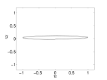
(a) $\omega=1$

(b) $\omega=0.1$

(c) $\omega=0.01$

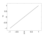
(d) $\omega=0.001$

Figure 2: Input-output curves for equation (1) with $c=15$ and $k=1$. The initial position is $(y,\dot{y})=(0,0)$ and the input is $u(t)=\sin(\omega t)$ for various frequencies $\omega$. The uncontrolled system has one equilibrium point. As $\omega\to 0,$ the loops disappear. This system does not display hysteresis.

Modify model (1) to obtain the nonlinear system

$$\ddot{y}(t)+c\dot{y}(t)+k\left(y(t)-y^{3}(t)\right)=u(t).$$ (4)

Setting $c=15$ and $k=-1$, the input-output curves with zero initial condition and periodic input are shown in Figure 3. It is clear from the figure that even for small $\omega$ a loop persists, which by Definition 2 indicates the presence of hysteresis. Observe also the differently shaped hysteresis loops for different inputs, which illustrate the complex behaviour of hysteresis, even for this second-order system.

System (4) also satisfies Definition 1. Rewriting (4) with no input $u$,

$$\dot{x}_{1}(t) =x_{2}(t)$$

$$\dot{x}_{2}(t) =-cx_{2}(t)-kx_{1}(t)+kx_{1}^{3}(t).$$

The equilibrium points are $(0,0)$ and $(\pm 1,0)$. The eigenvalues of the system linearized about $(\pm 1,0)$ have negative real part and hence $(\pm 1,0)$ are stable equilibrium points. This satisfies the first condition in Definition 1. (The equilibrium $(0,0)$ is unstable since one of its corresponding eigenvalues has positive real part.) Figure 4 demonstrates that the dynamics in equation (4) are independent of the rate at which inputs are varied given the range of frequencies. This satisfies the second condition in Definition 1. A similar example for the displacement of a magnetic beam is presented in [40, Example 4].

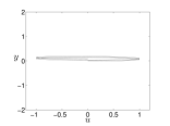
(a) $\omega=1$

(b) $\omega=0.1$

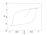
(c) $\omega=0.01$

(d) $\omega=0.001$

Figure 3: Input-output curves for the nonlinear system in (4) with $c=15$ and $k=-1$. The initial position is $(y,\dot{y})=(0,0)$ and the input is $u(t)=\sin(\omega t)$ for various $\omega$.

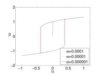
Figure 4: Input-output diagrams for the nonlinear system in (4) with $c=15$, $k=-1$. The initial position is $(y,\dot{y})=(0,0)$ and the input is $u(t)=\sin(\omega t)$ for $\omega\leq 0.0001$. At these low frequencies, the system exhibits rate independence.

Consider again the linear equation (1) but with $k=0$; that is

$$\ddot{y}(t)+c\dot{y}(t)=u(t).$$ (5)

and its corresponding unforced system in first-order form is

$$\dot{x}_{1}(t) =x_{2}(t)$$ (6a)

$$\dot{x}_{2}(t) ={-cx_{2}(t)}.$$ (6b)

The unforced system (6) has an infinite number of equilibria, $(a,0)$ where $a$ is any constant. The eigenvalues of (6) are $0$ and $-c$ and so the equilibrium points are stable if $c>0$.

For arbitrary initial conditions $(y(0),\dot{y}(0))=(y_{0},y_{1})$, the solution to (5) with $u(t)=\sin(\omega t)$ is

$$y(t) =y_{0}+\frac{y_{1}}{c}\left(1-e^{-ct}\right)-\frac{\sin(\omega t)}{\omega^{2}+c^{2}}$$

$$+\frac{\omega^{2}+c^{2}-c^{2}\cos(\omega t)-\omega^{2}e^{-ct}}{\omega c\left(\omega^{2}+c^{2}\right)}.$$

It follows that

$$\lim_{\omega\rightarrow 0}y(t)=y_{0}+\frac{y_{1}}{c}(1-e^{-ct})$$

and hence

$$\lim_{\underset{{\omega\rightarrow 0}}{t\rightarrow\infty}}y(t)=y_{0}+\frac{y_{1}}{c}.$$

The steady-state of (6) as $\omega\rightarrow 0$ depends on the initial conditions. Input-output curves are displayed in Figure 5 with $c=15$, zero initial condition and $u(t)=\sin(\omega t)$ for various values of the frequency $\omega$. The figures indicate that a loop persists as $\omega$ approaches $0$.

Note that the loop is a smooth circle, and does not display the same rapid transition as in Figures 3d and 4. The continuum of equilibrium points, rather than disconnected equilibrium points, may be the reason for the absence of sharp jumps. We will see in the next section that hysteresis in the Landau-Lifshitz equation behaves similarly.

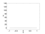
(a) $\omega=1$

(b) $\omega=0.1$

(c) $\omega=0.01$

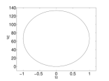
(d) $\omega=0.001$

Figure 5: Input-output curves for the linear system in (5). There are an infinite number of equilibria, $(a,0)$. The initial condition is $(y,\dot{y})=(0,0)$ and the input is $u(t)=\sin(\omega t)$ for various $\omega$.

III LANDAU-LIFSHITZ EQUATION

The Landau-Lifshitz equation is a coupled set of three nonlinear partial differential equations,

$$\dot{\mathbf{m}} =\mathbf{m}\times\mathbf{m}_{xx}-\nu\mathbf{m}\times\left(\mathbf{m}\times\mathbf{m}_{xx}\right)$$ (7a)

$$\mathbf{m}_{x}(0,t) =\mathbf{m}_{x}(L,t)=\mathbf{0}.$$ (7b)

$$\mathbf{m}(x,0) =\mathbf{m}_{0}(x)$$ (7c)

where $$\times L>0 \nu>0$$ indicates the vector cross product, is length and a material parameter. The solution to (7) is

$$\mathbf{m}(x,t)=(m_{1}(x,t),m_{2}(x,t),m_{3}(x,t))$$

for $$x\in[0,L]$$and

$$\mathbf{m}\times\mathbf{m}_{xx}= \left(\right.m_{2}m_{3}^{\prime\prime}-m_{3}m_{2}^{\prime\prime},$$

$$\left.-m_{1}m_{3}^{\prime\prime}+m_{3}m_{1}^{\prime\prime},m_{1}m_{2}^{\prime\prime}-m_{2}m_{1}^{\prime\prime}\right).$$

The prime notation indicates differentiation with respect to $$x \mathcal{L}_{2}^{3}=\mathcal{L}_{2}([0,L];\mathbb{R}^{3}).$$. Solutions to (7) are defined on Existence and uniqueness of solutions to (7) is shown in [25]. Equation (7) has been investigated in [20, 25], [35, Section 6.3.1].

On a molecular level, ferromagnets are divided into regions called magnetic domains. Each domain in a ferromagnet is magnetized to the same saturation, $M_{s}$. Mathematically, this means $||\mathbf{m}(x,t)||_{2}=M_{s}$ where $||\cdot||_{2}$ is the Euclidean norm. In much of the literature, $M_{s}$ is set to $1$ and the same convention is followed here; that is,

$$||\mathbf{m}(x,t)||_{2}=1$$ (7d)

and the initial condition $||\mathbf{m}_{0}(x)||_{2}=1$. The nonnegative parameter $\nu$ in (7a) is the damping parameter. It depends on the magnetization saturation and hence on the type of ferromagnet.

Theorem 3

The set of equilibrium solutions to the Landau-Lifshitz equation (7a) with Neumann boundary conditions (7b) is ${\mathbf{m}}(x)=\mathbf{a}$ where $\mathbf{a}\in\mathbb{R}^{3}$, $||\mathbf{a}||_{2}=1.$

Proof: It is shown in [35, Theorem 6.1.1] that the equilibrium solutions to (7a) are

$${\mathbf{m}}(x)=\mathbf{a}\cos(kx)+\mathbf{b}\sin(kx)$$

where $k\in\mathbb{R}$ is a constant, $\mathbf{a}=(a_{1},a_{2},a_{3})$ and $\mathbf{b}=(b_{1},b_{2},b_{3})$ for $a_{i},b_{i}\in\mathbb{R}$, $i=1,2,3$ constants with $||\mathbf{a}||_{2}=1,$ $||\mathbf{b}||_{2}=1$ and $\mathbf{a}^{\mathrm{T}}\mathbf{b}=0$. Applying the boundary conditions in (7b) implies $k=0$. $\Box$

Note that, as for the second-order linear example in (6), the Landau-Lifshitz equation has an infinite number of equilibria. The set of equilibrium points of (7) is

$$E= \{\mathbf{a}=(a_{1},a_{2},a_{3})\in\mathbb{R}^{3}:$$

$$a_{1},a_{2},a_{3}\mbox{ constants and }\mathbf{a}^{\mathrm{T}}\mathbf{a}=1\}.$$ (8)

Theorem 4

[35, Proposition 6.2.1] Each point in the equilibrium set $E$ (III) is stable in the $\mathcal{L}_{2}^{3}$-norm.

If we introduce the notion of an equilibrium set, then $E$ can be shown to be asymptotically stable [29].

Since the Landau-Lifshitz equation has an infinite number of stable equilibria, Definition 1 suggests it exhibits hysteresis.

Consider the Landau-Lifshitz equation with input $\mathbf{u}(t)$:

$$\dot{\mathbf{m}}=\mathbf{m}\times\mathbf{m}_{xx}-\nu\mathbf{m}\times\left(\mathbf{m}\times\mathbf{m}_{xx}\right)+{\mathbf{u}}(t).$$

The input is chosen to be ${\mathbf{u}}(t)=\left(0.001\cos(\omega t),0,0\right)$; that is, there is a time-varying magnetic field in the $m_{1}$ direction and no magnetic field in the $m_{2}$ and $m_{3}$.

(a) $\omega=1$

(b) $\omega=0.1$

(c) $\omega=0.01$

(d) $\omega=0.001$

Figure 6: Hysteresis loops for $m_{1}(x,t)$ of the (nonlinear) Landau-Lifshitz equation with $x=0.6$ and $\nu=0.02$. The input is $\mathbf{u}(t)=\left(0.001\cos(\omega t),0,0\right)$. The initial condition is $\mathbf{m}_{0}(x)=\left(1,0,0\right)$.

The hysteresis loops for $m_{1}(x,t)$ with $x$ fixed is illustrated in Figure 6. The initial condition is $\mathbf{m}_{0}(x)=\left(1,0,0\right)$, $\nu=0.02$ and $L=1$. It is clear from Figure 6 that the input-output curves exhibit persistent loops as the frequency of the input approaches zero. In a similar manner, $m_{2}$ and $m_{3}$ also exhibit persistent loops. Thus, these simulations indicate that the Landau-Lifshitz equation satisfies Definition 2.

Note that the hysteresis loops in Figure 6 have the same appearance as those in Figure 5 for the second-order linear example (6). In both examples there is a continuum of equilibrium points.

To obtain the linear Landau-Lifshitz equation, equation (7a) is rewritten in semilinear form,

$$\frac{\partial\mathbf{m}}{\partial t}=\nu\mathbf{m}_{xx}+\mathbf{m}\times\mathbf{m}_{xx}+\nu\left|\left|\mathbf{m}_{x}\right|\right|_{2}^{2}\mathbf{m},$$ (9)

using equation (7d) and properties of cross products. Then substitute $\mathbf{m}(x,t)={\mathbf{a}}+\mathbf{z}(x,t)$ where $\mathbf{a}\in E$ is an equilibrium of (7) and $\mathbf{z}\in\mathcal{L}_{2}^{3}$ is a small perturbation into (9). Defining

$$A\mathbf{z}=\nu\mathbf{z}_{xx}+\mathbf{a}\times\mathbf{z}_{xx}$$

with domain

$$D(A)=\{ \mathbf{z}:\mathbf{z}\in\mathcal{L}_{2}^{3},\,\,\mathbf{z}_{x}\in\mathcal{L}_{2}^{3},\,\,\mathbf{z}_{xx}\in\mathcal{L}_{2}^{3},$$

$$\mathbf{z}_{x}(0,t)=\mathbf{0}=\mathbf{z}_{x}(L,t)\},$$

the Landau-Lifshitz equation linearized about an equilibrium $\mathbf{a}$ is

$$\dot{\mathbf{z}} =A\mathbf{z},\quad\mathbf{z}(0)=\mathbf{z}_{0}$$ (10a)

$$\mathbf{z}_{x}(0,t) =\mathbf{0}=\mathbf{z}_{x}(L,t).$$ (10b)

The operator $A$ can be shown to generate an analytic semigroup [29]. Therefore, (10) is a well-posed system.

Theorem 5

Any constant $\mathbf{c}\in\mathbb{R}^{3}$ is a stable equilibrium of (10).

Proof: A brief outline is given here; details can be found in [29]. Since $A$ generates an analytic semigroup, the spectrum determined growth assumption is satisfied and so the eigenvalues of $A$ determine the stability of the linear system (10) [33, Section 5.1], [38, Section 3.2].

It is clear that any constant function $\mathbf{c}$ is an equilibrium of (10). Let $\lambda\in\mathbb{C}$. The eigenvalue problem of (10) is $\lambda\mathbf{v}=A\mathbf{v}$ and boundary conditions $\mathbf{v}_{x}(0)=\mathbf{v}_{x}(L)=\mathbf{0}$. where $\mathbf{v}\in\mathcal{L}_{2}^{3}$. Solving, the eigenvalues of (10) are $\lambda_{1}=0$ and for $n\in\mathbb{Z}$,

$$\lambda_{2}^{+,-} =\frac{-(1+2n)^{2}\pi^{2}\nu}{L^{2}}\pm i\frac{(1+2n)^{2}\pi^{2}}{L^{2}},$$

$$\lambda_{3} =\frac{-(1+2n)^{2}\pi^{2}\nu}{L^{2}},$$

$$\lambda_{4}^{+,-} =\frac{-(2n)^{2}\pi^{2}\nu}{L^{2}}\pm i\frac{(2n)^{2}\pi^{2}}{L^{2}},$$

$$\lambda_{5} =\frac{-(2n)^{2}\pi^{2}\nu}{L^{2}}.$$

Since all the eigenvalues have nonpositive real part, the equilibria of (10) are stable. $\Box$

Based on the result in Theorem 5, Definition 1 indicates that the linear Landau-Lifshitz equation exhibits hysteresis. We now look at periodic inputs to determine whether persistent loops exists and Definition 2 is satisfied. Again, $\nu=0.02$, $L=1$, and the same periodic input is applied as for the nonlinear Landau-Lifshitz equation. Figure 7 shows the input-output curves for the linear Landau-Lifshitz equation with $\mathbf{a}=(1,0,0)$ and initial condition $\mathbf{z}_{0}(x)=\left(1,0,0\right)$. A loop does persist as the frequency of the input approaches zero. Similar plots are obtained when control is on the second and third components. The hysteresis loops in Figure 7 are similar in shape to the nonlinear Landau-Lifshitz equation depicted in Figure 6 and the example in (6), each of which have a continuum of equilibria.

(a) $\omega=1$

(b) $\omega=0.1$

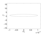
(c) $\omega=0.01$

(d) $\omega=0.001$

Figure 7: Hysteresis loops for $z_{1}(x,t)$ of the linear Landau-Lifshitz equation with $x=0.6$ and $\nu=0.02$. The linearization is at $\mathbf{a}=(1,0,0)$. The input is $\mathbf{u}(t)=\left(0.001\cos(\omega t),0,0\right)$ and the initial condition is $\mathbf{z}_{0}(x)=\left(1,0,0\right)$.

IV CONCLUSIONS

The results here indicate that existence of multiple stable equilibria is crucial for systems to be hysteretic. The linear and nonlinear Landau-Lifshitz equations exhibit hysteretic behaviour. Hysteresis was also shown in a second-order linear differential equation. Since hysteretic behaviour was displayed by several linear systems, this suggests that multiple stable equilibria, not nonlinearity, are the key factors leading to the display of hysteresis in systems. As well, an absence of jumps in the hysteresis loops were observed. Further investigation is required to determine whether this is always the case for systems with a zero eigenvalue.

In [30], the authors discuss controlling hysteresis in the Landau-Lifshitz equation; that is controlling between equilibrium points.

References

- [17] T. Aiki and E. Minchev. A prey-predator model with hysteresis effect. SIAM Journal on Mathematical Analysis, 36(6):2020 – 2032, 2005.
- [18] M. Alimov. Asymptotic analysis of the joining of an ice-rock body in flow through porous media. Fluid Dyn. (USA), 38(1):78 – 87, 2003.
- [19] M. Alimov, K. Kornev, and G. Mukhamadullina. Hysteretic effects in the problems of artificial freezing. SIAM Journal on Applied Mathematics, 59(2):387–410, 1998.
- [20] F. Alouges and A. Soyeur. On global weak solutions for Landau-Lifshitz equations: existence and nonuniqueness. Nonlinear Anal., 18(11):1071–1084, 1992.
- [21] D. Bernstein. Ivory ghost. IEEE Control. Sys. Mag., 27:17–18, 2007.
- [22] G. Bertotti. Hysteresis in Magnetism. Academic Press Limited, 1998.
- [23] M. Brokate and J. Sprekels. Hysteresis and Phase Transitions. Springer-Verlag New York, Inc, 1996.
- [24] G. Carbou, M. A. Efendiev, and P. Fabrie. Relaxed model for the hysteresis in micromagnetism. Proc. Roy. Soc. Edinburgh Sect. A, 139(4):759–773, 2009.
- [25] G. Carbou and P. Fabrie. Regular solutions for Landau-Lifschitz equation in a bounded domain. Differential Integral Equations, 14(2):213–229, 2001.
- [26] G. Carbou and S. Labbé. Stability for static walls in ferromagnetic nanowires. Discrete Contin. Dyn. Syst. Ser. B, 6(2):273–290 (electronic), 2006.
- [27] G. Carbou and S. Labbé. Stability for walls in ferromagnetic nanowire. In Numerical mathematics and advanced applications, pages 539–546. Springer, Berlin, 2006.
- [28] G. Carbou, S. Labbé, and E. Trélat. Control of travelling walls in a ferromagnetic nanowire. Discrete and Continuous Dynamical Systems. Series S, 1(1):51–59, 2008.
- [29] A. Chow. Control of hysteresis in the Landau-Lifshitz Equation. PhD thesis, University of Waterloo, 2013.
- [30] A. Chow and K. Morris. Control of hysteresis in the landau-lifshitz equation. Automatica, submitted.
- [31] H. Christenson. Confinement effects on freezing and melting. Journal of Physics Condensed Matter, 13(11):R95 – R133, 2001.
- [32] R. Cowburn, D. Koltsov, A. Adeyeye, M. Welland, and D. Tricker. Single-domain circular nanomagnets. Physical Review Letters, 83(5):1042 – 1045, 1999.
- [33] R. Curtain and H. Zwart. An introduction to Infinite-Dimensional Linear Systems Theory, volume 21 of Texts in Applied Mathematics. Springer-Verlag, 1995.
- [34] Y. Gou, A. Goussev, J. Robbins, and V. Slastikov. Stability of precessing domain walls in ferromagnetic nanowires. Phys. Rev. B, Condens. Matter Mater. Phys. (USA), 84(10):104445 (7 pp.), 2011.
- [35] B. Guo and S. Ding. Landau-Lifshitz Equations, volume 1 of Frontier Of Research with the Chinese Academy of Sciences. World Scientific, 2008.
- [36] F. Ikhouane. Characterization of hysteresis processes. Mathematics of Control, Signals & Systems, 25:291–310, 2013.
- [37] B. Jayawardhana, H. Logemann, and E. Ryan. Pid control of second-order systems with hysteresis. Int. J. Control (UK), 81(8):1331 – 42, 2008.
- [38] Z. H. Luo, B. Z. Guo, and O. Morgul. Stability and Stabilization of Infinite Dimensional Systems with Applications. Communications and Control Engineering. Springer, 1999.
- [39] I. D. Mayergoyz, C. Serpico, and G. Bertotti. On stability of magnetization dynamics in nanoparticles. IEEE Transactions on Magnetics, 46(6):1718 – 1721, 2010.
- [40] K. Morris. What is hysteresis? Applied Mechanics Reviews, 64(5), 2011.
- [41] J. Murray. Mathematical Biology. Springer-Verlag, second edition, 1993.
- [42] S. J. Noh, Y. Miyamoto, M. Okuda, N. Hayashi, and Y. K. Kim. Control of magnetic domains in co/pd multilayered nanowires with perpendicular magnetic anisotropy. Journal of Nanoscience and Nanotechnology, 12(1):428 – 432, 2012.
- [43] J. Oh and D. Bernstein. Semilinear Duhem model for rate-independent and rate-dependent hysteresis. IEEE Trans. Autom. Control (USA), 50(5):631 – 45, 2005.
- [44] O. Petrov and I. Furo. Curvature-dependent metastability of the solid phase and the freezing-melting hysteresis in pores. PHYSICAL REVIEW E, 73(1, Part 1), 2006.
- [45] C. Schneider and S. Winchell. Hysteresis in conducting ferromagnets. Physica B (Netherlands), 372(1-2):269 – 72, 2006.
- [46] R. Smith. Smart Material Systems. Frontiers in Applied Mathematics. SIAM Frontiers, 2005.
- [47] S. Valadkhan, K. Morris, and A. Khajepour. Review and comparison of hysteresis models for magnetostrictive materials. Journal of Intelligent Material Systems and Structures, 20:131–142, 2009.
- [48] S. Valadkhan, K. Morris, and A. Khajepour. Stability and robust position control of hysteretic systems. International Journal of Robust and Nonlinear Control, 20(4):460 – 471, 2010.
- [49] B. Van De Wiele, L. Dupra, and F. Olyslager. Memory properties in a Landau-Lifshitz hysteresis model for thin ferromagnetic sheets. Journal of Applied Physics, 99(8), 2006.
- [50] B. Van De Wiele, F. Olyslager, and L. Dupre. Fast semianalytical time integration schemes for the landau-lifshitz equation. IEEE Transactions on Magnetics, 43(6):2917 – 2919, 2007.
- [51] A. Visintin. On the preisach model for hysteresis. Nonlinear Analysis, 8(9):977–996, 1984.
- [52] A. Visintin. Mathematical models of hysteresis. In G. Bertotti and I. Mayergoyz, editors, The Science of Hysteresis. Academic Press, 2006.
- [53] J. A. Walker. On the application of Liapunov’s direct method to linear dynamical systems. J. Math. Anal. Appl., 53(2):187–220, 1976.
- [54] B. Yang and Y. Zhao. Coercivity control in finite arrays of magnetic particles. Journal of Applied Physics, 110(10), 2011.