Waterfilling Theorems for Linear Time-Varying Channels and Related Nonstationary Sources

Abstract

The capacity of the linear time-varying (LTV) channel, a continuous-time LTV filter with additive white Gaussian noise, is characterized by waterfilling in the time–frequency plane. Similarly, the rate distortion function for a related nonstationary source is characterized by reverse waterfilling in the time–frequency plane. Constraints on the average energy or on the squared-error distortion, respectively, are used. The source is formed by the white Gaussian noise response of the same LTV filter as before. The proofs of both waterfilling theorems rely on a Szegő theorem for a class of operators associated with the filter. A self-contained proof of the Szegő theorem is given. The waterfilling theorems compare well with the classical results of Gallager and Berger. In the case of a nonstationary source, it is observed that the part of the classical power spectral density is taken by the Wigner–Ville spectrum. The present approach is based on the spread Weyl symbol of the LTV filter, and is asymptotic in nature. For the spreading factor, a lower bound is suggested by means of an uncertainty inequality.

I Introduction

The characterization of the capacity of continuous-time channels with an average power constraint by waterfilling in the frequency domain, going back to Shannon [1], has been given by Gallager [2] for linear time-invariant (LTI) channels in great generality. At least since the advent of mobile communications, there has been a vivid interest in similar results for LTV channels; see [3], [4], [5], [6] to cite only a few. Although most wireless communication channels are modeled by random LTV filters [7], [6], a waterfilling characterization of the capacity of deterministic LTV channels might also be of interest. Furthermore, many nonstationary continuous-time sources can be described as the response of an LTV filter to white Gaussian noise. It is therefore natural to ask for a solution to the dual problem, namely the reverse waterfilling characterization of the rate distortion function for such sources with a fidelity criterion. The classical answer to this question in the case of a stationary source, already outlined by Kolmogorov in [8], has been given by Berger [9] for a broad class of stationary random processes. Since then, until quite recently [10], no similar results for nonstationary sources have been reported. Within the framework of time–frequency analysis, treating the time–frequency plane “as a whole” [11], we present waterfilling solutions to both problems (with constraints on the average energy in the case of the channel and on the squared-error distortion in the case of the source).

We consider integral operators $\boldsymbol{P}$ from the Hilbert space $L^{2}(\mathbb{R})$ of square-integrable functions $f:\mathbb{R}\rightarrow\mathbb{C}\cup\{\infty\}$ into itself of the form

$$(\boldsymbol{P}f)(t)=\int_{-\infty}^{\infty}h(t,t^{\prime})f(t^{\prime})\,\mathrm{d}t^{\prime}$$ (1)

with the kernel $h\in L^{2}(\mathbb{R}^{2})$, i.e., Hilbert–Schmidt (HS) operators on $L^{2}(\mathbb{R})$ [13]. Every such operator has a unique Weyl symbol $p=\sigma_{\boldsymbol{P}}\in L^{2}(\mathbb{R}^{2})$ so that Eq. (1) may be written as [14], [15]

$$(\boldsymbol{P}f)(t)=\frac{1}{2\pi}\iint_{\mathbb{R}^{2}}p\left(\frac{t+t^{\prime}}{2},\omega\right)\mathrm{e}^{\mathrm{i}(t-t^{\prime})\omega}f(t^{\prime})\,\mathrm{d}t^{\prime}\,\mathrm{d}\omega.$$ (2)

The Weyl symbol, a concept originating in quantum mechanics [16], [17], [18], is now a standard tool for the description of LTV systems [19] (because of its physical provenance, we shall often switch between variables $t,\omega$ and $x,\xi$ standing for time, angular frequency and the corresponding phase space coordinates). The operator (1), regarded as an LTV filter for finite-energy signals $f(t)$, will play a central role in our investigations. However, for the formulation of problems it will be necessary to replace $\boldsymbol{P}$ with the operator $\boldsymbol{P}_{r}:L^{2}(\mathbb{R})\rightarrow L^{2}(\mathbb{R})$ having the spread Weyl symbol $\sigma_{\boldsymbol{P}_{r}}(t,\omega)=p_{r}(t,\omega)\triangleq p(t/r,\omega/r)$, where $r\geq 1$ is the spreading factor. Eq. (1) then turns into

$$(\boldsymbol{P}_{r}f)(t)=\int_{-\infty}^{\infty}h(r,t,t^{\prime})f(t^{\prime})\,\mathrm{d}t^{\prime},$$ (3)

where $h(r,\cdot,\cdot)\in L^{2}(\mathbb{R}^{2})$ denotes the kernel, now depending on $r$. It is not difficult to express $h(r,t,t^{\prime})$ in terms of $h(t,t^{\prime})$ and $r$; however, we shall rarely make use of that representation since the Weyl symbol appears to be the appropriate filter description in our context. Although other choices are possible for that symbol (also called the time–frequency transfer function; see [19] for a systematic overview), the Weyl symbol excels due to some unique properties, one of them being most helpful later on. There is one other choice for the description of LTV filters: the spreading function [7], [18], [19]. This is the two-dimensional (symplectic) Fourier transform of, in our case, the Weyl symbol $\sigma_{\boldsymbol{P}}$,

$$\hat{\sigma}_{\boldsymbol{P}}(\tau,\nu)=\frac{1}{2\pi}\iint_{\mathbb{R}^{2}}\mathrm{e}^{-\mathrm{i}(x\nu-\tau\xi)}\sigma_{\boldsymbol{P}}(x,\xi)\,\mathrm{d}x\,\mathrm{d}\xi,$$

and its popularity in mobile communications comes from the fact that the representation

$$(\boldsymbol{P}f)(t)=\frac{1}{2\pi}\iint_{\mathbb{R}^{2}}\hat{\sigma}_{\boldsymbol{P}}(\tau,\nu)\mathrm{e}^{-\mathrm{i}\tau\nu/2}f(t-\tau)\mathrm{e}^{\mathrm{i}t\nu}\,\mathrm{d}\tau\,\mathrm{d}\nu$$

allows a simple interpretation of the operator in terms of a weighted superposition of time delays $\tau$ and Doppler shifts $\nu$ of the input signal. Because of $\hat{\sigma}_{\boldsymbol{P}_{r}}(\tau,\nu)=r^{2}\hat{\sigma}_{\boldsymbol{P}}(r\tau,r\nu)$ we observe increasing concentration of the spreading function $\hat{\sigma}_{\boldsymbol{P}_{r}}$ of operator $\boldsymbol{P}_{r}$ around the origin of the $\tau,\nu$-plane as $r\rightarrow\infty$. This behaviour, shared by many practical LTV filters and termed underspread in [20], [19], is therefore also peculiar to our setting (where, in principle, $r$ tends to infinity). However, it remains to be remarked that the spreading function would not be the proper means for formulating the subsequent waterfilling theorems, Theorem 2 and Theorem 3.

The present paper evolves from previous work presented in [12]. We now give a brief overview of the contributions of our paper with emphasis on extensions and modifications compared to [12]; for details, refer to the text. The LTV filters, initially arbitrary HS operators, are later restricted to those having Weyl symbols in the Schwartz space of rapidly decreasing functions (thus including the bivariate Gaussian function used in [12]). The waterfilling theorem for the capacity of the LTV channel is now stated in terms of the reciprocal squared modulus of the spread Weyl symbol of the LTV filter. Similarly, the reverse waterfilling theorem for the rate distortion function for the nonstationary source is stated in terms of the squared modulus of the spread Weyl symbol of the LTV filter. A major difference from [12] is the statement of a new Szegő theorem, which is now general enough to cover a large class of operators. For part of the proof of the Szegő theorem we resort to a powerful asymptotic expansion having its roots in semiclassical physics [16], [17], [21]. Since our results are asymptotic in nature, there is a need to give a lower bound for the spreading factor so that the formulas in the waterfilling theorems yield useful approximations. A lower bound is suggested by means of the Robertson–Schrödinger uncertainty inequality [16]. Several concrete examples will illustrate our results.

II Mathematical Preliminaries

In the present section, we fix the notation and compile some mathematical concepts and results associated with the LTV filter (3). In Section II-B, it will be sufficient to restrict ourselves to the spreading factor $r=1$, therefore it is omitted; generalizations to the case $r\geq 1$, mostly obvious, will be addressed as needed in the subsequent sections.

II-A Notation

The following notations will be adopted: The inner product in $L^{2}(\mathbb{R})$ is denoted by $\langle f_{1},f_{2}\rangle=\int_{-\infty}^{\infty}f_{1}(x)\overline{f_{2}(x)}\,\mathrm{d}x$, and $\|f\|=\langle f,f\rangle^{1/2}$ is the corresponding norm. For an operator $\boldsymbol{A}:L^{2}(\mathbb{R})\rightarrow L^{2}(\mathbb{R})$, its adjoint $\boldsymbol{A}^{*}:L^{2}(\mathbb{R})\rightarrow L^{2}(\mathbb{R})$ is defined by the condition $\langle\boldsymbol{A}f_{1},f_{2}\rangle=\langle f_{1},\boldsymbol{A}^{*}f_{2}\rangle\,\forall f_{1},f_{2}\in L^{2}(\mathbb{R})$; $\boldsymbol{A}$ is called self-adjoint if $\boldsymbol{A}^{*}=\boldsymbol{A}$. $\mathscr{S}(\mathbb{R}^{n}),\,n=1,2,$ is the Schwartz space of rapidly decreasing functions on $\mathbb{R}^{n}$ (cf. [18]); if $n=2$ and the function $u$ additionally depends on the parameter $r$, $u=u(r,x,\xi)$, then $u\in\mathscr{S}(\cdot,\mathbb{R}^{2})$ means

$$\sup_{x,\xi}|x^{\beta_{1}}\xi^{\beta_{2}}\partial_{x}^{\alpha_{1}}\partial_{\xi}^{\alpha_{2}}u(r,x,\xi)|\leq C_{\boldsymbol{\alpha}\boldsymbol{\beta}}<\infty$$

for all $\boldsymbol{\alpha}=(\alpha_{1},\alpha_{2}),\boldsymbol{\beta}=(\beta_{1},\beta_{2})\in\mathbb{N}_{0}^{2}$, where the constants $C_{\boldsymbol{\alpha}\boldsymbol{\beta}}$ do not depend on $r$. $L^{2}_{\mathbb{R}}(\mathbb{R})$ is the real Hilbert space of real-valued functions in $L^{2}(\mathbb{R})$.

II-B Fundamental Concepts and Results

II-B1 Weyl correspondence

The Weyl symbol $\sigma_{\boldsymbol{P}}$ of the HS operator $\boldsymbol{P}$ in (1) is given by the equation (sometimes called the Wigner transform) [14], [15]

$$\sigma_{\boldsymbol{P}}(x,\xi)=\int_{-\infty}^{\infty}\mathrm{e}^{-\mathrm{i}\xi x^{\prime}}h\left(x+\frac{x^{\prime}}{2},x-\frac{x^{\prime}}{2}\right)\,\mathrm{d}x^{\prime}.$$ (4)

The linear mapping $\boldsymbol{P}\mapsto p=\sigma_{\boldsymbol{P}}$ defined by (4) establishes a one-to-one correspondence between all HS operators on $L^{2}(\mathbb{R})$ and all functions $p\in L^{2}(\mathbb{R}^{2})$ [14], [18]. Moreover, it holds (here and hereafter, double integrals extend over $\mathbb{R}^{2}$)

$$\frac{1}{2\pi}\iint|p(x,\xi)|^{2}\,\mathrm{d}x\,\mathrm{d}\xi=\iint|h(x,y)|^{2}\,\mathrm{d}x\,\mathrm{d}y.$$ (5)

The above mapping (or rather its inverse) is called Weyl correspondence [18].

II-B2 Singular value decomposition (SVD)

Every HS operator $\boldsymbol{P}$ on $L^{2}(\mathbb{R})$ is compact and so is its adjoint $\boldsymbol{P}^{*}$ [13]. Define the self-adjoint operator $\boldsymbol{A}\triangleq\boldsymbol{P}^{*}\boldsymbol{P}$ on $L^{2}(\mathbb{R})$. $\boldsymbol{A}$ is positive because $\langle\boldsymbol{A}f,f\rangle=\langle\boldsymbol{P}f,\boldsymbol{P}f\rangle\geq 0\,\forall f\in L^{2}(\mathbb{R})$, and compact since one factor, say, $\boldsymbol{P}$, is compact. Therefore, $\boldsymbol{P}$ has the SVD [13], [2, Th. 8.4.1]

$$(\boldsymbol{P}f)(x)=\sum_{k=0}^{N}\sqrt{\lambda_{k}}\,\langle f,f_{k}\rangle g_{k}(x),$$ (6)

where $\{f_{0},\ldots,f_{N}\}$, $\{g_{0},\ldots,g_{N}\}$ ($N\in\mathbb{N}_{0}$ or $N=\infty$) form orthonormal systems in $L^{2}(\mathbb{R})$, and $\lambda_{0}\geq\lambda_{1}\geq\ldots>0$ are the non-zero eigenvalues of $\boldsymbol{A}$ (counting multiplicity) with the corresponding eigenfunctions $f_{k}$; the functions $g_{k}$ are defined by $g_{k}=\boldsymbol{P}f_{k}/\sqrt{\lambda_{k}}$, the positive numbers $\sqrt{\lambda_{k}},\,k=0,\ldots,N$, being the non-zero singular values of $\boldsymbol{P}$. If $\boldsymbol{P}$ maps $L^{2}_{\mathbb{R}}(\mathbb{R})$ into itself, then the functions $f_{k},g_{k}$ will be real-valued. Without loss of generality (w.l.o.g.) we shall assume that $N=\infty$ (otherwise, put $\lambda_{k}=0$ and choose $f_{k},g_{k}$ anyway for $k>N$). Then always $\lambda_{k}\rightarrow 0$ as $k\rightarrow\infty$.

II-B3 Traces of operators

By Eq. (6), the kernel of operator $\boldsymbol{P}$ in (1) has the form $h(x,y)=\sum_{k=0}^{\infty}\sqrt{\lambda_{k}}g_{k}(x)\overline{f_{k}(y)}$ from where we readily obtain $\iint|h(x,y)|^{2}\,\mathrm{d}x\,\mathrm{d}y=\sum_{k=0}^{\infty}\lambda_{k}$. In combination with (5), this results in the useful equation

$$\mathrm{tr}\,\boldsymbol{A}\triangleq\sum_{k=0}^{\infty}\lambda_{k}=\frac{1}{2\pi}\iint|p(x,\xi)|^{2}\,\mathrm{d}x\,\mathrm{d}\xi<\infty.$$ (7)

Since $\mathrm{tr}\,\boldsymbol{A}$ (the trace of $\boldsymbol{A}$) is finite, $\boldsymbol{A}$ is of trace class (see [13] for a general definition of trace class operators).

In Section VI, the operator $\boldsymbol{\tilde{A}}\triangleq\boldsymbol{P}\boldsymbol{P}^{*}$ will be considered. Plugging $\boldsymbol{P}^{*}f\in L^{2}(\mathbb{R})$ for $f\in L^{2}(\mathbb{R})$ in (6) we get for $\boldsymbol{\tilde{A}}$ the representation $(\boldsymbol{\tilde{A}}f)(x)=\int K_{\boldsymbol{\tilde{A}}}(x,y)f(y)\,\mathrm{d}y$ with the kernel

$$K_{\boldsymbol{\tilde{A}}}(x,y)=\sum_{k=0}^{\infty}\lambda_{k}g_{k}(x)\overline{g_{k}(y)}.$$ (8)

$\boldsymbol{\tilde{A}}$ has the same eigenvalues as $\boldsymbol{A}$. Furthermore, since we are dealing with the Weyl symbol we have the simple rule

$$\sigma_{\boldsymbol{P}^{*}}(x,\xi)=\overline{\sigma_{\boldsymbol{P}}(x,\xi)}.$$ (9)

Hence, Eq. (7) holds by analogy for operator $\boldsymbol{\tilde{A}}$ (just replace “$\boldsymbol{A}$” with “$\boldsymbol{\tilde{A}}$”).

In quantum mechanics, an operator on $L^{2}(\mathbb{R})$ is called a density operator, if it is 1) self-adjoint, 2) positive and 3) of trace class with trace one [16]. Apparently, the above operators $\boldsymbol{A},\boldsymbol{\tilde{A}}$ enjoy all these properties, with the exception of the very last. We give them a name:

Definition 1

A quasi density operator (QDO) is an operator on $L^{2}(\mathbb{R})$ of the form $\boldsymbol{P}^{*}\!\boldsymbol{P}$ or $\boldsymbol{P}\boldsymbol{P}^{*}$, where $\boldsymbol{P}:L^{2}(\mathbb{R})\rightarrow L^{2}(\mathbb{R})$ is an HS operator.

Remark 1

In [22] it is noted that any self-adjoint, positive operator on $L^{2}(\mathbb{R})$ of trace class allows factorizations as given in Def. 1; the above narrow-sense meaning of QDO will be sufficient for our purposes.

The following result is key to our paper: If the operator $\boldsymbol{B}:L^{2}(\mathbb{R})\rightarrow L^{2}(\mathbb{R})$ has a Weyl symbol $\sigma_{\boldsymbol{B}}\in\mathscr{S}(\mathbb{R}^{2})$, then $\boldsymbol{B}$ is of trace class and its trace is given by the trace rule [23]

$$\mathrm{tr}\,\boldsymbol{B}=\frac{1}{2\pi}\iint\sigma_{\boldsymbol{B}}(x,\xi)\,\mathrm{d}x\,\mathrm{d}\xi.$$ (10)

Refer to [16] concerning the smoothness assumption and for a proof.

II-B4 Bound on eigenvalues

If the function $a=a(x,\xi):\mathbb{R}^{2}\rightarrow\mathbb{C}$ is differentiable up to the sixth order and it holds

$$\sup_{x,\xi}|\partial_{x}^{\alpha_{1}}\partial_{\xi}^{\alpha_{2}}a(x,\xi)|\leq C_{\boldsymbol{\alpha}}<\infty$$ (11)

for all $\boldsymbol{\alpha}=(\alpha_{1},\alpha_{2})\in I=\{0,1,2,3\}^{2}$, then the operator $\boldsymbol{A}$ defined by the Weyl symbol $a$ is a bounded operator from $L^{2}(\mathbb{R})$ into itself, and it holds

$$\|\boldsymbol{A}f\|\leq c_{0}C\,\|f\|,\,f\in L^{2}(\mathbb{R}),$$

where $C=\sum_{\boldsymbol{\alpha}\in I}C_{\boldsymbol{\alpha}}$ and $c_{0}$ is a certain constant not depending on the operator. This is the famous theorem of Calderón–Vaillancourt [24], [17]. Consequently, the absolute value $|\lambda|$ of every eigenvalue $\lambda$ of $\boldsymbol{A}$ is bounded by $c_{0}C$.

III Channel Model and Discretization

We consider for any spreading factor $r\geq 1$ held constant the LTV channel

$$\tilde{g}(t)=(\boldsymbol{P}_{r}f)(t)+n(t),\,-\infty<t<\infty,$$ (12)

where $\boldsymbol{P}_{r}$ is the LTV filter (3), the real-valued filter input signals $f(t)$ are of finite energy and the noise signals $n(t)$ at the filter output are realizations of white Gaussian noise with two-sided power spectral density (PSD) $N_{0}/2=\theta^{2}>0$. Moreover, we assume throughout that the kernel $h(t,t^{\prime})$ of operator $\boldsymbol{P}$ in (1) is real-valued; observe that due to

$$h(r,t,t^{\prime})=rh((r^{-1}(t+t^{\prime})+r(t-t^{\prime}))/2,\\ (r^{-1}(t+t^{\prime})-r(t-t^{\prime}))/2),$$

then also the kernel $h(r,t,t^{\prime})$ of operator $\boldsymbol{P}_{r}$ will be real-valued so that $\boldsymbol{P}_{r}$ maps $L^{2}_{\mathbb{R}}(\mathbb{R})$ into itself. This channel is depicted in Fig. 1.

We now reduce the LTV channel (12) to a (discrete) vector Gaussian channel, following the approach in [2] for LTI channels; our analysis is greatly simplified by the restriction to finite-energy input signals. For the SVD of operator $\boldsymbol{P}_{r}$ the $r$-dependent operator $\boldsymbol{A}(r)\triangleq\boldsymbol{P}_{r}\!\!^{*}\boldsymbol{P}_{r}$ has to be considered; since eigenvalues $\lambda_{k}$ and (eigen-)functions $f_{k},\,g_{k}$ in the SVD now also depend on $r$, this will be indicated by a superscript $\cdot\,^{(r)}$. Then, by Eq. (6), the LTV filter (3) has the SVD

$$(\boldsymbol{P}_{r}f)(t)=\sum_{k=0}^{\infty}[\lambda_{k}^{(r)}]^{\frac{1}{2}}a_{k}\,g_{k}^{(r)}\!(t),$$ (13)

where the coefficients are $a_{k}=\langle f,f_{k}^{(r)}\rangle,\,k=0,1,\ldots,$ and $\{g_{k}^{(r)};k=0,1,\ldots\}$ forms an orthonormal system in $L^{2}(\mathbb{R})$. Recall from Section II-B2 that the functions $f_{k}^{(r)}\!,\,g_{k}^{(r)}$ are real-valued. The perturbed filter output signal $g=\boldsymbol{P}_{r}f$, $\tilde{g}(t)=g(t)+n(t)$, is passed through a bank of matched filters with impulse responses $h_{k}(t)=g_{k}^{(r)}(-t),\,k=0,1,\ldots\,.$ The matched filter output signals are sampled at time zero to yield $\langle\tilde{g}(t),h_{k}(-t)\rangle=b_{k}+n_{k}$, where $b_{k}=\langle g(t),h_{k}(-t)\rangle=[\lambda_{k}^{(r)}]^{1/2}a_{k}$, and the detection errors $n_{k}=\langle n(t),h_{k}(-t)\rangle$ are realizations of independent identically distributed (i.i.d.) zero-mean Gaussian random variables $N_{k}$ with the variance $\theta^{2}$, $N_{k}\sim\mathcal{N}(0,\theta^{2})$. From the detected values $\hat{b}_{k}=b_{k}+n_{k}$ we get the estimates $\hat{a}_{k}=[\lambda_{k}^{(r)}]^{-1/2}\hat{b}_{k}=a_{k}+z_{k}$ for the coefficients $a_{k}$ of the input signal $f$, where $z_{k}$ are realizations of independent Gaussian random variables $Z_{k}\sim\mathcal{N}(0,\theta^{2}/\lambda_{k}^{(r)})$. Thus, we are led to the infinite-dimensional vector Gaussian channel

$$Y_{k}=X_{k}+Z_{k},\,k=0,1,\ldots,$$ (14)

where the noise $Z_{k}$ is distributed as described. Note that the noise PSD $\theta^{2}$, measured in watts/Hz, also has the physical dimension of an energy.

Figure 1: Model of the LTV channel. The Weyl symbol $p_{r}(t,\omega)$ acts as a time–frequency transfer function; $r\geq 1$ is the spreading factor.

Figure 2: Model of the nonstationary source

IV A Szegő Theorem for Quasi Density Operators

From now on to the end of the paper, we assume that the Weyl symbol $p$ of the HS operator $\boldsymbol{P}$ in (2) is in the Schwartz space of rapidly decreasing functions, $p\in\mathscr{S}(\mathbb{R}^{2})$.

Consider the QDO $\boldsymbol{A}=\boldsymbol{P}^{*}\!\boldsymbol{P}$ and generalize it as above to the operator $\boldsymbol{A}(r)=\boldsymbol{P}_{r}\!\!^{*}\boldsymbol{P}_{r}$, $r\geq 1$ (being again a QDO). We now state and prove a Szegő theorem for $\boldsymbol{A}(r)$. Szegő theorems like the subsequent Theorem 1 are not new [25], [23], [27], [26], but all the Szegő theorems we are aware of are inadequate for our purposes. The proof of Lemma 2 (see below) rests on an asymptotic expansion of the $n$th power of $\boldsymbol{A}(r)$. Asymptotic expansions such as that (there are different kinds of estimating the error!) have a long tradition in semiclassical physics and the theory of pseudodifferential operators [25], [17]; rigorous proofs, however, are sometimes hard to find. A complete proof of the following Lemma 1, which is perhaps closest to results of [21], is shifted to the Appendix. Although we need the lemma only in the case of $m=1$, it would not be natural to omit a full statement of it:

Lemma 1

For any $n\in\mathbb{N}$, the Weyl symbol of the operator $\boldsymbol{A}^{n}(r)\triangleq[\boldsymbol{A}(r)]^{n},\,r\geq 1,$ has the asymptotic expansion

$$\sigma_{\boldsymbol{A}^{n}(r)}(x,\xi)\sim\sum_{k=0}^{\infty}r^{-2k}a_{k}(x/r,\xi/r),$$ (15)

where $a_{0}(x,\xi)=|p(x,\xi)|^{2n}$, $a_{k}\in\mathscr{S}(\mathbb{R}^{2})$ else, and Eq. (15) means that for all $m\in\mathbb{N}$ it holds

$$\sigma_{\boldsymbol{A}^{n}(r)}(x,\xi)=\sum_{k=0}^{m-1}r^{-2k}a_{k}(x/r,\xi/r)\\ +r^{-2m}R_{m}(r,x/r,\xi/r),$$ (16)

where $R_{m}=R_{m}(r,x,\xi)\in\mathscr{S}(\cdot,\mathbb{R}^{2})$.

Proof:

See Appendix. ∎

Asymptotically, i.e., as $r\rightarrow\infty$, $a_{0}(x/r,\xi/r)$ is the dominant part of the asymptotic expansion (15). As customary in the theory of pseudodifferential operators (cf., e.g., [17], [23]), the expression $|p_{r}(x,\xi)|^{2n}$ will be called the principal symbol of operator $\boldsymbol{A}^{n}(r)$. Observe that the Weyl symbol of the $n$th power of the operator $\boldsymbol{\tilde{A}}(r)=\boldsymbol{P}_{r}\boldsymbol{P}_{r}^{*},r\geq 1,$ has an asymptotic expansion analogous to that of $\boldsymbol{A}^{n}(r)$ and the principal symbols of both operators are identical.

Definition 2

For any two functions $A,\,B:[1,\infty)\rightarrow\mathbb{R}$ the notation $A\doteq B$ means

$$\lim_{x\rightarrow\infty}\frac{A(x)-B(x)}{x^{2}}=0,$$

or, equivalently, $A(x)=B(x)+o(x^{2})$ as $x\rightarrow\infty$, where $o(\cdot)$ denotes the standard Landau little-o symbol.

In our context, $x$ will always be the spreading factor $r\geq 1$. Thus $A\doteq B$ implies that $A(r)/r^{2}=B(r)/r^{2}+\epsilon$ where $\epsilon\rightarrow 0$ as $r\rightarrow\infty$.

Lemma 2

For any polynomial $G_{N}(x,z)=\sum_{n=1}^{N}c_{n}(x)z^{n}$ with bounded variable coefficients $c_{n}(x)\in\mathbb{R},\,x\geq 1,$ it holds

$$\sum_{k=0}^{\infty}G_{N}(r,\lambda_{k}^{(r)})\doteq\frac{1}{2\pi}\iint_{\mathbb{R}^{2}}G_{N}(r,|p_{r}(x,\xi)|^{2})\,\mathrm{d}x\,\mathrm{d}\xi.$$

Proof:

First, application of operator $\boldsymbol{P}_{r}^{*}$ to both sides of Eq. (13) yields

$$\boldsymbol{A}(r)f=\sum_{k=0}^{\infty}\lambda_{k}^{(r)}\langle f,f_{k}^{(r)}\rangle f_{k}^{(r)}.$$

So we get for any $f\in L^{2}(\mathbb{R})$ the expansion

$$G_{N}(r,\boldsymbol{A}(r))f=\sum_{k=0}^{\infty}G_{N}(r,\lambda_{k}^{(r)})\langle f,f_{k}^{(r)}\rangle f_{k}^{(r)}.$$

Hence, operator $\boldsymbol{B}(r)\triangleq G_{N}(r,\boldsymbol{A}(r))$ is of trace class with the trace

$$\mathrm{tr}\,\boldsymbol{B}(r)=\sum_{k=0}^{\infty}G_{N}(r,\lambda_{k}^{(r)}),$$ (17)

the series being absolutely converging since $G_{N}(x,0)=0\,\forall x\in[1,\infty)$.

Second, we use the trace rule (10) to obtain

$$\mathrm{tr}\,\boldsymbol{B}(r)=\frac{1}{2\pi}\iint\sigma_{\boldsymbol{B}(r)}(x,\xi)\,\mathrm{d}x\,\mathrm{d}\xi,$$ (18)

where $\sigma_{\boldsymbol{B}(r)}(x,\xi)$ is the Weyl symbol of operator $\boldsymbol{B}(r)$. By linearity of the Weyl correspondence, $\sigma_{\boldsymbol{B}(r)}(x,\xi)$ has the expansion

$$\sigma_{\boldsymbol{B}(r)}(x,\xi)=\sum_{n=1}^{N}c_{n}(r)\sigma_{\boldsymbol{A}^{n}(r)}(x,\xi).$$ (19)

From Lemma 1, taking $m=1$, we infer that

$$\iint\sigma_{\boldsymbol{A}^{n}(r)}(x,\xi)\,\mathrm{d}x\,\mathrm{d}\xi\doteq\iint|p_{r}(x,\xi)|^{2n}\,\mathrm{d}x\,\mathrm{d}\xi.$$

Plugging (19) into (18), we obtain by means of the latter equation

$$\mathrm{tr}\,\boldsymbol{B}(r) =\frac{1}{2\pi}\sum_{n=1}^{N}c_{n}(r)\iint\sigma_{\boldsymbol{A}^{n}(r)}(x,\xi)\,\mathrm{d}x\,\mathrm{d}\xi$$

$$\doteq\frac{1}{2\pi}\sum_{n=1}^{N}c_{n}(r)\iint|p_{r}(x,\xi)|^{2n}\,\mathrm{d}x\,\mathrm{d}\xi$$

$$=\frac{1}{2\pi}\iint G_{N}(r,|p_{r}(x,\xi)|^{2})\,\mathrm{d}x\,\mathrm{d}\xi.$$ (20)

Eq. (20) in combination with Eq. (17) concludes the proof. ∎

Lemma 1 shows that in the case of $n=1$ and, say, $m=1$, the Weyl symbol $a(r,x,\xi)=\sigma_{\boldsymbol{A}(r)}(x,\xi)$ of operator $\boldsymbol{A}(r)$ satisfies Ineq. (11) of Section II-B4 with upper bounds $C_{\boldsymbol{\alpha}}$ that may be chosen independent of $r\geq 1$. Consequently, the eigenvalues $\lambda_{k}^{(r)}$ of $\boldsymbol{A}(r)$ are uniformly bounded for $r\geq 1$; define

$$\Lambda_{p}\triangleq\max\left\{\sup_{\,r\geq 1}\lambda_{0}^{(r)},\max_{x,\xi}|p(x,\xi)|^{2}\right\}.$$ (21)

This constant appears in the next theorem:

Theorem 1 (Szegő Theorem)

Let $g:[0,\Delta]\rightarrow\mathbb{R}$, $\Delta\in(0,\infty)$, be a continuous function such that $\lim_{x\rightarrow 0+}g(x)/x$ exists. For any functions $a,\,b:[1,\infty)\rightarrow\mathbb{R}$, where $a(x)$ is bounded and $\Lambda_{p}b(x)\in[0,\Delta]$, define the function $G(x,z)=a(x)g(b(x)z),\,(x,z)\in[1,\infty)\times[0,\Lambda_{p}]$. Then it holds

$$\sum_{k=0}^{\infty}G(r,\lambda_{k}^{(r)})\doteq\frac{1}{2\pi}\iint_{\mathbb{R}^{2}}G(r,|p_{r}(x,\xi)|^{2})\,\mathrm{d}x\,\mathrm{d}\xi.$$ (22)

Proof:

The function $f(x)=g(x)/x,\,x\in(0,\Delta],$ has a continuous extension $F(x)$ onto the compact interval $[0,\Delta]$. By virtue of the Weierstrass approximation theorem, for any $m\in\mathbb{N}$ there exists a polynomial $F_{N_{m}-1}(x)$ of some degree $N_{m}-1$ such that $|F(x)-F_{N_{m}-1}(x)|\leq\epsilon_{m}=\frac{1}{m}$ for all $x\in[0,\Delta]$. Consequently, the polynomial $g_{N_{m}}(x)=xF_{N_{m}-1}(x)$ of degree $N_{m}$ satisfies the inequality

$$|g(x)-g_{N_{m}}(x)|\leq\epsilon_{m}x,\,x\in[0,\Delta].$$ (23)

Define the polynomial with variable coefficients $G_{N_{m}}(x,z)=a(x)\,g_{N_{m}}\!(b(x)z)$. We now show that

$$r^{-2}\sum_{k=0}^{\infty}G_{N_{m}}(r,\lambda_{k}^{(r)})\rightarrow r^{-2}\sum_{k=0}^{\infty}G(r,\lambda_{k}^{(r)})$$ (24)

and

$$\frac{r^{-2}}{2\pi}\iint G_{N_{m}}(r,|p_{r}(x,\xi)|^{2})\,dx\,d\xi$$ (25)

$$\rightarrow \frac{r^{-2}}{2\pi}\iint G(r,|p_{r}(x,\xi)|^{2})\,dx\,d\xi$$

as $m\rightarrow\infty$, uniformly for all $r\geq 1$ . To this end, first observe that by Eq. (7) (generalized to the operator $\boldsymbol{P}_{r},r\geq 1$) it holds

$$\begin{split}\sum_{k=0}^{\infty}\lambda_{k}^{(r)}&=\frac{1}{2\pi}\iint|p_{r}(x,\xi)|^{2}\,\mathrm{d}x\,\mathrm{d}\xi\\ &=c_{p}r^{2},\end{split}$$ (26)

where $c_{p}=(2\pi)^{-1}\iint|p(x,\xi)|^{2}\,\mathrm{d}x\,\mathrm{d}\xi$ is a finite constant.

Proof of (24): By Ineq. (23) we get (precluding the trivial case $\Lambda_{p}=0$)

$$|\sum_{k=0}^{\infty}G(r,\lambda_{k}^{(r)})-\sum_{k=0}^{\infty}G_{N_{m}}(r,\lambda_{k}^{(r)})|$$

$$\leq \sum_{k=0}^{\infty}|G(r,\lambda_{k}^{(r)})-G_{N_{m}}(r,\lambda_{k}^{(r)})|$$

$$\leq M\epsilon_{m}(\Delta/\Lambda_{p})\sum_{k=0}^{\infty}\lambda_{k}^{(r)},$$

where $M=\sup_{x\geq 1}|a(x)|<\infty$. Since $\sum_{k=0}^{\infty}\lambda_{k}^{(r)}=c_{p}r^{2}$, after division of the inequality by $r^{2}$, convergence in (24) follows as claimed.

Proof of (25): Similarly,

$$|\iint G(r,|p_{r}(x,\xi)|^{2})\,dx\,d\xi$$

$$-\iint G_{N_{m}}(r,|p_{r}(x,\xi)|^{2})\,dx\,d\xi|$$

$$\leq M\epsilon_{m}(\Delta/\Lambda_{p})\iint|p_{r}(x,\xi)|^{2}\,dx\,d\xi.$$

Since $(2\pi)^{-1}\iint|p_{r}(x,\xi)|^{2}\,dx\,d\xi=c_{p}r^{2}$, after division by $2\pi r^{2}$ we come to the same conclusion as before.

Finally, choose a (large) number $m\in\mathbb{N}$, so that the left-hand sides in (24), (25) become arbitrarily close to their respective limits. Replace function $G$ in Eq. (22) with the polynomial $G_{N_{m}}$. Then, by Lemma 2 and the uniform convergence in (24), (25) the theorem follows. ∎

Note that Theorem 1 applies to operator $\boldsymbol{\tilde{A}}(r)$ without any changes.

V Waterfilling Theorem for the Capacity of Linear Time-Varying Channels

V-A Waterfilling in the Time–Frequency Plane

The function $N_{r},r\geq 1,$ occurring in the next theorem is defined by $N_{r}(t,\omega)=N_{1}(t/r,\omega/r)$ where

$$N_{1}(t,\omega)=\frac{\theta^{2}}{2\pi}\,|p(t,\omega)|^{-2},$$ (27)

$p=\sigma_{\boldsymbol{P}}$ being the Weyl symbol of operator $\boldsymbol{P}$. Recall that $p\in\mathscr{S}(\mathbb{R}^{2})$. $O(\cdot)$ denotes the standard Landau big-O symbol and $x^{+}$ denotes the positive part of $x\in\mathbb{R}$, $x^{+}=\max\{0,x\}$.

Theorem 2

Assume that the average energy $S$ of the input signal depends on $r$ such that $S(r)=O(r^{2})$ as $r\rightarrow\infty$. Then for the capacity (in nats per transmission) of the LTV channel (12) it holds

$$C\doteq\frac{1}{2\pi}\iint_{\mathbb{R}^{2}}\frac{1}{2}\ln\left(1+\frac{(\nu-N_{r}(t,\omega))^{+}}{N_{r}(t,\omega)}\right)\,\mathrm{d}t\,\mathrm{d}\omega,$$ (28)

where $\nu$ is chosen so that

$$S\doteq\iint_{\mathbb{R}^{2}}(\nu-N_{r}(t,\omega))^{+}\,\mathrm{d}t\,\mathrm{d}\omega.$$ (29)

Proof:

The first part of the proof is accomplished by waterfilling on the noise variances [2, Th. 7.5.1]. Let $\nu_{k}^{2}=\theta^{2}/\lambda_{k}^{(r)}(\mbox{put }\theta^{2}/0=\infty),\,k=0,1,\ldots,$ be the noise variance in the $k$th subchannel of the discretized LTV channel (14). We exclude the trivial case $S=0$. The “water level” $\sigma^{2}$ is then uniquely determined by the condition

$$S=\sum_{k=0}^{\infty}(\sigma^{2}-\nu_{k}^{2})^{+}=\sum_{k=0}^{K-1}(\sigma^{2}-\nu_{k}^{2}),$$ (30)

where $K=\max\{k\in\mathbb{N};\nu_{k-1}^{2}<\sigma^{2}\}$ is the number of subchannels in the resulting finite-dimensional vector Gaussian channel. The capacity $C$ of that vector channel is achieved when the components $X_{k}$ of the input vector $(X_{0},\ldots,X_{K-1})$ are independent random variables $\sim\mathcal{N}(0,\sigma^{2}-\nu_{k}^{2})$; then

$$C=\sum_{k=0}^{K-1}\frac{1}{2}\ln\left(1+\frac{\sigma^{2}-\nu_{k}^{2}}{\nu_{k}^{2}}\right)\quad\mathrm{nats}.$$ (31)

In the second part of the proof we apply the above Szegő theorem, Theorem 1. To start with, note that $\sigma^{2}$ is dependent on $r$ and that always $\sigma^{2}=\sigma^{2}(r)>0$. Additionally, suppose for the time being that the function $\sigma^{2}(r)$ is finitely upper bounded as $r\rightarrow\infty$. Define

$$\ln_{+}x=\left\{\!\!\begin{array}[]{cl}\max\{0,\ln x\}&\mbox{if }x>0,\\ 0&\mbox{if }x=0.\end{array}\right.$$ (32)

By Eq. (31) we now have

$$C =\sum_{k=0}^{\infty}\frac{1}{2}\ln_{+}\left(\frac{\sigma^{2}(r)}{\theta^{2}}\lambda_{k}^{(r)}\right)$$

$$=\sum_{k=0}^{\infty}a(r)g(b(r)\lambda_{k}^{(r)}),$$

where $a(r)=1$, $b(r)=\sigma^{2}(r)/\theta^{2}$, $g(x)=\frac{1}{2}\ln_{+}x,x\in[0,\Delta]$, and $\Delta$ is chosen so that $\Lambda_{p}b(r)\leq\Delta<\infty$ when $r$ is large enough, $\Lambda_{p}$ being the constant (21). This choice is possible since $\sigma^{2}(r)$ remains bounded as $r\rightarrow\infty$; w.l.o.g., we assume $\Lambda_{p}b(r)\in[0,\Delta]$ for all $r\geq 1$. Then, by Theorem 1 it follows that $C=C(r)$ satisfies

$$C \doteq\frac{1}{2\pi}\iint\frac{1}{2}\ln_{+}\left(\frac{\sigma^{2}(r)}{\theta^{2}}\,|p_{r}(x,\xi)|^{2}\right)\,\mathrm{d}x\,\mathrm{d}\xi$$

$$=\frac{1}{2\pi}\iint\frac{1}{2}\ln\!\left[1+\frac{\left(\frac{\sigma^{2}(r)}{2\pi}-N_{r}(t,\omega)\right)^{+}}{N_{r}(t,\omega)}\right]\!\mathrm{d}t\,\mathrm{d}\omega,$$ (33)

where $N_{r}(t,\omega)=\frac{\theta^{2}}{2\pi}\,|p_{r}(t,\omega)|^{-2}$. Next, rewrite Eq. (30) as

$$S=\sum_{k=0}^{\infty}\sigma^{2}(r)\left(1-\frac{1}{\frac{\sigma^{2}(r)}{\theta^{2}}\lambda_{k}^{(r)}}\right)^{+}.$$

Put $a(r)=\sigma^{2}(r)$, $b(r)=\sigma^{2}(r)/\theta^{2}$ and define

$$g(x)=\left\{\!\!\begin{array}[]{cl}\left(1-\frac{1}{x}\right)^{+}&\mbox{if }x>0,\\ 0&\mbox{if }x=0.\end{array}\right.$$

Again, w.l.o.g., we may assume that $a(r)$ is bounded and $\Lambda_{p}b(r)\in[0,\Delta]$ for all $r\geq 1$ where $\Delta$ is chosen as above. Then, by Theorem 1 it follows that

$$S \doteq\frac{1}{2\pi}\iint\sigma^{2}(r)\left(1-\frac{1}{\frac{\sigma^{2}(r)}{\theta^{2}}\,|p_{r}(x,\xi)|^{2}}\right)^{+}\,\mathrm{d}x\,\mathrm{d}\xi$$

$$=\iint\left(\frac{\sigma^{2}(r)}{2\pi}-N_{r}(t,\omega)\right)^{+}\,\mathrm{d}t\,\mathrm{d}\omega.$$ (34)

Finally, replacement of $\frac{\sigma^{2}(r)}{2\pi}$ in Eqs. (33), (34) by parameter $\nu$ yields Eqs. (28), (29).

We complete the proof by a bootstrap argument: Take Eq. (29) as a true equation and use it for the definition of $\sigma^{2}(=2\pi\nu)$; after a substitution we obtain

$$\iint(\nu-N_{1}(t,\omega))^{+}\,\mathrm{d}t\,\mathrm{d}\omega=S(r)/r^{2}.$$

Because of the growth condition imposed on $S$, $\nu=\nu(r)$ stays below a finite upper bound as $r\rightarrow\infty$, and so does $\sigma^{2}(r)$. Consequently, the previous argument applies and the capacity $C$ is given by Eq. (28). Second, by reason of Theorem 1, it holds for the actual average input energy $S_{\mathrm{act}}(r)$ $=\sum_{k=0}^{\infty}(\sigma^{2}(r)-\nu_{k}^{2})^{+}$ that $S_{\mathrm{act}}\doteq S$. Thus, the dotted equation (29) applies anyway—even when $S$ is taken as $S_{\mathrm{act}}$. ∎

From the property $p\in\mathscr{S}(\mathbb{R}^{2})$ it is easily deduced that, say,

$$N_{1}(t,\omega)\geq c_{1}(t^{2}+\omega^{2}),\,(t,\omega)\in\mathbb{R}^{2},$$

where $c_{1}$ is some positive constant depending on $p$; therefore, condition (29) certainly makes sense.

Note that the use of Landau symbols in Theorem 2 does not mean that we need to pass to the limit (here, as $r\rightarrow\infty$). Rather, the dotted equations (28), (29) may give useful approximations even when $r$ is finite (but large enough).

Example 1

Consider the HS operator $\boldsymbol{P}$ on $L^{2}(\mathbb{R})$ with the bivariate Gaussian function

$$p(t,\omega)=\mathrm{e}^{-\frac{1}{2}(\gamma^{-2}t^{2}+\gamma^{2}\omega^{2})},$$ (35)

$\gamma>0$ fixed, as the Weyl symbol. Then $\boldsymbol{P}_{r},r\geq 1,$ has the Weyl symbol $p_{r}(t,\omega)=\exp[-(\gamma^{-2}t^{2}+\gamma^{2}\omega^{2})/(2r^{2})]$. $\boldsymbol{P}_{r}$ is related to the operator $\boldsymbol{P}_{\delta}^{(\gamma)}$ of the so-called heat channel [12] by the equation $\boldsymbol{P}_{r}=c\,\boldsymbol{P}_{\delta}^{(\gamma)}$, where $\delta=2\,\mathrm{arccoth}(2r^{2})>0$ and $c=\cosh(\delta/2)$. $\boldsymbol{P}^{(\gamma)}_{\delta}$ has the diagonalization [11], [28], [12]

$$(\boldsymbol{P}_{\delta}^{(\gamma)}f)(t)=\sum_{k=0}^{\infty}\rho^{k+\frac{1}{2}}\langle f,f_{k}\rangle f_{k}(t),$$

where $\rho=\mathrm{e}^{-\delta}$ and $f_{k}(t)=(D_{\gamma}H_{k})(t)\triangleq\gamma^{-\frac{1}{2}}H_{k}(t/\gamma)$ is the dilated $k$th Hermite function $H_{k}(t)$; the real-valued eigenfunctions $f_{k},\,k=0,1,\ldots,$ form an orthonormal system in $L^{2}(\mathbb{R})$. Therefore, $\boldsymbol{A}(r)=\boldsymbol{P}_{r}\!\!^{*}\boldsymbol{P}_{r}=\boldsymbol{P}_{r}^{2}$ has the eigenvalues $\lambda_{k}^{(r)}=c^{2}\rho^{2k+1},k=0,1,\ldots,$ so that the LTV channel (12) reduces to the discrete vector channel (14) where the noise random variables $Z_{k}\sim\mathcal{N}(0,\nu_{k}^{2})$ have the variances $\nu_{k}^{2}=(\theta/c)^{2}\rho^{-2k-1}$. Take the average input energy $S(r)=2\pi r^{2}\theta^{2}\,\mathrm{SNR}$, where $\mathrm{SNR}>0$ is the signal-to-noise ratio ($2\pi r^{2}\theta^{2}$ having the interpretation of the average energy of the relevant noise). In Fig. 3, capacity values labeled “exact” have been computed numerically by waterfilling on the noise variances, as given in the proof of Theorem 2. Note that the results do not depend on $\theta^{2}$.

From Theorem 2, after computation of the double integrals and elimination of parameter $\nu$ we get the equation

$$C\doteq\frac{r^{2}}{8}\left[\mathrm{W}_{0}((4\pi\,\mathrm{SNR}-1)/\mathrm{e})+1\right]^{2},$$ (36)

where $\mathrm{W}_{0}$ is the principal branch of the Lambert W function determined by the conditions $\mathrm{W}(x)\exp[\mathrm{W}(x)]=x$ for all $x\in[-\mathrm{e}^{-1},\infty)$ and $\mathrm{W}(0)=0$ [29], [30]. In Fig. 3, the approximate capacity (36) is plotted as a function of $r$ (labeled “waterfilling”). Surprisingly, the approximation is good even for spreading factors close to one.

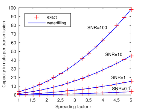
Figure 3: Exact values and waterfilling approximation of the capacity of the LTV channel of Example 1

V-B Operational Meaning of the Capacity Result

Theorem 2 gives the information capacity (in the sense of [31]) of the LTV channel (12). To provide this result with an operational meaning, we need to construct a code in the form of a set of continuous-time signals which achieves a rate arbitrarily close to this capacity along with constructive methods of encoding and decoding.

We use the notation in the proof of Theorem 2. For any fixed average input energy $S>0$ and any spreading factor $r\geq 1$ held constant, the construction will be based on the eigenfunctions $f_{k}^{(r)}\!,\,k=0,\ldots,K-1$, of operator $\boldsymbol{A}(r)=\boldsymbol{P}_{r}\!\!^{*}\boldsymbol{P}_{r}$, where $K$ is as in Eq. (30); at the receiver, the corresponding functions $g_{k}^{(r)}=\boldsymbol{P}_{r}f_{k}^{(r)}\!/[\lambda_{k}^{(r)}]^{\frac{1}{2}}$ will be used. Since the functions $g_{k}^{(r)}\!,f_{k}^{(r)}$ are in the range of the operators $\boldsymbol{P}_{r},\boldsymbol{P}_{r}^{*}$ with Weyl symbols $p_{r},\bar{p}_{r}\in\mathscr{S}(\mathbb{R}^{2})$, resp., these functions are rapidely decreasing, $g_{k}^{(r)}\!,f_{k}^{(r)}\in\mathscr{S}(\mathbb{R})$. In practice, any finite collection of functions $u_{1},\ldots,u_{N}\in\mathscr{S}(\mathbb{R})$ may be regarded to be concentrated on a common bounded interval centered at the origin and to be almost zero outside. Thus, for the sake of simplicity, we shall assume that $f_{k}^{(r)}(t)=g_{k}^{(r)}(t)=0,\,k=0,\ldots,K-1,$ if $|t|\geq d/2$ for some $d\in(0,\infty)$; $d$ will have the meaning of a delay later on. It will be convenient to switch from natural logarithms to logarithms to the base 2 and so from nats to bits. Then, the (information) capacity $C_{k}$ of the $k$th subchannel, $k=0,\ldots,K-1$, figuring in the sum on the right-hand side of Eq. (31), reads

$$C_{k}=\frac{1}{2}\log_{2}\left(1+\frac{\sigma^{2}-\nu_{k}^{2}}{\nu_{k}^{2}}\right)\quad\mathrm{bits}.$$

We treat the $K$ subchannels as independent Gaussian channels with the noise variance $\nu_{k}^{2}$ each and follow the classical approach of Shannon [1], [31]: For the $k$th subchannel, for any rate $R_{k}$ with $0<R_{k}<C_{k}$ and any $\epsilon>0$ generate a codebook $\{\boldsymbol{a}_{k}(m)=(a_{k0}(m),\ldots,a_{k,L_{k}-1}(m));\,m=1,2,\ldots,M_{k}\triangleq 2^{\lfloor R_{k}L_{k}\rfloor}\}\subseteq\mathbb{R}^{L_{k}}$ with the property that 1) $a_{kl}(m),l=0,\ldots,L_{k}-1$, are realizations of i.i.d. random variables $\sim\mathcal{N}(0,\sigma^{2}-\nu_{k}^{2})$ and 2) the probability of a maximum likelihood decoding error is smaller than $\epsilon$ for every transmitted codeword $\boldsymbol{a}_{k}(m),m=1,2,\ldots,M_{k}$. We may assume that $L_{0}=\ldots=L_{K-1}=L$. For every message $\boldsymbol{m}=(m_{0},\ldots,m_{K-1})\in\{1,2,\ldots,M_{0}\}\times\ldots\times\{1,2,\ldots,M_{K-1}\}$ form the pulses

$$u_{l}(\boldsymbol{m},t-ld)=\sum_{k=0}^{K-1}a_{kl}(m_{k})f_{k}^{(r)}(t-ld),\,l=0,\ldots,L-1,$$

and take the pulse train

$$u(\boldsymbol{m},t)=\sum_{l=0}^{L-1}u_{l}(\boldsymbol{m},t-ld)$$ (37)

as input signal to the physical channel. During transmission over that channel, each pulse $u_{l}(\boldsymbol{m},t-ld)$ undergoes a distortion modeled by the LTV filter (3), and results in the deformed pulse

$$v_{l}(\boldsymbol{m},t-ld)=\sum_{k=0}^{K-1}[\lambda_{k}^{(r)}]^{\frac{1}{2}}a_{kl}(m_{k})g_{k}^{(r)}(t-ld).$$

Thus, the output signal of the physical channel is

$$y(\boldsymbol{m},t)=\sum_{l=0}^{L-1}v_{l}(\boldsymbol{m},t-ld)+n(t),$$

where $n(t)$ is a realization of white Gaussian noise as in the LTV channel model (12). For any of the $K$ subchannels, pass the signal $y(\boldsymbol{m},t)$ through the matched filter with impulse response $h_{k}(t)$ as given in Section III; sample the matched filter output signal at time $ld,\,l=0,\ldots,L-1$. Since $y(\boldsymbol{m},t)=v_{l}(\boldsymbol{m},t-ld)+n(t)$ if $|t-ld|\leq d/2$, we again obtain estimates $\hat{a}_{kl}(m_{k})=a_{kl}(m_{k})+z_{kl}$ for $a_{kl}(m_{k})$, where $z_{kl}$ are realizations of independent Gaussian random variables $\sim\mathcal{N}(0,\nu_{k}^{2})$. Maximum likelihood decoding of the perturbed codeword $\tilde{\boldsymbol{a}}_{k}(m_{k})\triangleq(\hat{a}_{k0}(m_{k}),\ldots,\hat{a}_{k,L-1}(m_{k}))$ yields the correct codeword $\boldsymbol{a}_{k}(m_{k})$ (thus, $m_{k}$) with a probability of error smaller than $\epsilon$. At the transmitter, choose the message $\boldsymbol{m}$ at random such that each component $m_{k}$ has probability $M_{k}^{-1}$ and is independent of the other components; convey $\boldsymbol{m}$ through a pulse train as described. Then—treating each of the $K$ subchannels separately—the total rate $R_{\mathrm{tot}}=\frac{1}{L}\sum_{k=0}^{K-1}\lfloor R_{k}L\rfloor$ (in bits per pulse) is attained with a total probability of a decoding error smaller than $K\epsilon$. When $L\rightarrow\infty$, Shannon’s theory [1] ensures that $\epsilon$ can be made as small as we wish. Moreover, $R_{\mathrm{tot}}\rightarrow R\triangleq R_{0}+\ldots+R_{K-1}$ and, by the law of large numbers, the average input energy $\frac{1}{L}\sum_{l=0}^{L-1}\sum_{k=0}^{K-1}a_{kl}^{2}(m_{k})$ tends to $\sum_{k=0}^{K-1}(\sigma^{2}-\nu_{k}^{2})=S$ with probability 1. Finally, since the rate $R$ may be chosen arbitrarily close to the capacity $C=C_{0}+\ldots+C_{K-1}$ (at the expense of a larger length $L$ of the pulse train), the construction of the desired coding system is complete.

Example 2

Consider the LTV channel (12) with the operator $\boldsymbol{P}_{r}=c\,\boldsymbol{P}^{(\gamma)}_{\delta}$ of Example 1. The eigenfunctions of operator $\boldsymbol{A}(r)=\boldsymbol{P}_{r}\!\!^{*}\boldsymbol{P}_{r}$ are the functions $f_{k}^{(r)}(t)=f_{k}(t)=(D_{\gamma}H_{k})(t),\,k=0,1,\ldots,$ (here, not depending on $r$); the functions $g_{k}^{(r)}$ in the SVD (13) of $\boldsymbol{P}_{r}$ coincide with $f_{k}^{(r)}$ for all $k$. Now, choose specifically $r=2,\,\gamma=1/10$ and take the average input energy $S=2\pi r^{2}\theta^{2}\,\mathrm{SNR}$ (as generally assumed in Example 1) with $\mathrm{SNR}=100$ and noise PSD $N_{0}/2=\theta^{2}=0.01$ (unit omitted). Waterfilling on the noise variances $\nu_{k}^{2}=(\theta/c)^{2}\rho^{-2k-1}(\rho=\mathrm{e}^{-\delta}),\,k=0,1,\ldots,$ as given in the proof of Theorem 2, yields the number of $K=11$ subchannels. In Fig. 4(a), the first $K$ eigenfunctions $f_{k}^{(r)}(t)=(D_{\gamma}H_{k})(t),\,k=0,\ldots,K-1,$ are displayed. The portion of an input pulse train plotted in Fig. 4(b) has been computed according to Eq. (37) with the delay parameter $d=6a$, $a=\sqrt{2}r\gamma$, by numerical simulation of the involved random variables. Observe that there is no appreciable overlap of individual pulses. Each pulse transmits 22.6 bits ($=$15.7 nats, cf. Fig. 3) of information arbitrarily reliably [provided that the length of the pulse train(s) becomes larger and larger]. The meaning of parameter $a$ will be explained in Section VII.

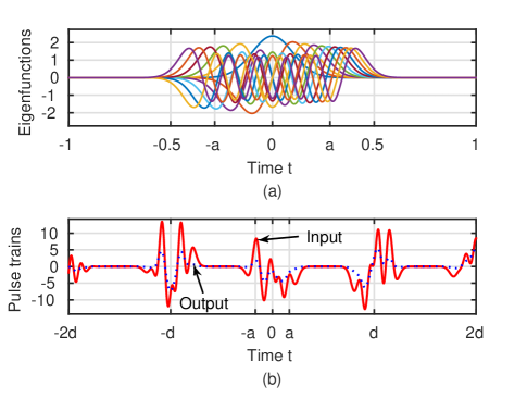
Figure 4: (a) First eleven eigenfunctions, dilated Hermite functions, for the LTV channel of Example 2. (b) Portion of an input pulse train (centered at the origin) to the physical channel and the corresp. distorted output (without noise) of the same example. Time $t$ is measured in some unit of time; on the $y$-axis, also the physical dimension is omitted.

V-C Comparison with Classical Work

Gallager’s theorem [2, Th. 8.5.1] gives the capacity of LTI channels under very general assumptions. In the case of an LTI filter with a bounded and square-integrable frequency response $H(\omega)=\int_{-\infty}^{\infty}\mathrm{e}^{-\mathrm{i}\omega t}h(t)\,\mathrm{d}t$ (a.k.a. transfer function; $h\not=0$ is the impulse response) and additive white Gaussian noise of PSD $N_{0}/2=\theta^{2}>0$ at the filter output, Gallager’s theorem states that the capacity (in bits per second) is given parametrically by

$$C =\frac{1}{2\pi}\int_{-\infty}^{\infty}\frac{1}{2}\log_{2}\left(1+\frac{(\nu-N(\omega))^{+}}{N(\omega)}\right)\,\mathrm{d}\omega$$ (38)

$$S =\int_{-\infty}^{\infty}(\nu-N(\omega))^{+}\,\mathrm{d}\omega,$$ (39)

where $\nu$ is the parameter, $S$ is average input power, and

$$N(\omega)=\frac{\theta^{2}}{2\pi}\,|H(\omega)|^{-2}.$$ (40)

We observe a perfect formal analogy between the waterfilling formulas (38), (39) and those in Theorem 2. Moreover, the functions (40) and (27) are the reciprocal squared modulus of the (time–frequency) transfer function of the respective filter times the same noise figure.

Eqs. (28), (29) may also be used, of course, for a parametric representation of the function $C(S)$ with $\nu$ as parameter.

VI Reverse Waterfilling Theorem for Related Nonstationary Sources

In the present section, we consider the nonstationary source formed by the nonstationary zero-mean Gaussian process given by the Karhunen–Loève expansion

$$X(t)=\sum_{k=0}^{\infty}X_{k}\,g_{k}^{(r)}(t),\,t\in\mathbb{R},$$ (41)

where the coefficients $X_{k},\,k=0,1,\ldots,$ are independent random variables $\sim\mathcal{N}(0,\sigma_{k}^{2})$ with the variances $\sigma_{k}^{2}=\sigma^{2}\lambda_{k}^{(r)},\,\sigma>0$. This is the response of the LTV filter (13) to white Gaussian noise with PSD $N_{0}/2=\sigma^{2}$; cf. [2]. This source is depicted in Fig. 2.

VI-A Wigner–Ville Spectrum of the Source

In the present subsection, the spreading factor $r\geq 1$ is initially not essential, hence set to one and not displayed.

The Wigner–Ville spectrum (WVS) $\Phi(t,\omega)$ of the nonstationary random process $\{X(t),t\in\mathbb{R}\}$ in (41) describes its density of (mean) energy in the time–frequency plane [32]. The WVS may be regarded as the nonstationary counterpart to the PSD of a stationary random process. It is defined by means of the Wigner distribution $Wx$ of the realizations $x(t)$ of $\{X(t)\}$ and then taking the expectation [32]. Since $x(t)$ is almost surely in $L^{2}(\mathbb{R})$, we may write

$$(Wx)(t,\omega)=\frac{1}{2\pi}\int_{-\infty}^{\infty}\mathrm{e}^{-\mathrm{i}\omega t^{\prime}}x\left(t+\frac{t^{\prime}}{2}\right)\overline{x\left(t-\frac{t^{\prime}}{2}\right)}\mathrm{d}t^{\prime}.$$

The WVS $\Phi(t,\omega)=\mathsf{E}[(WX)(t,\omega)]$ of the random process $\{X(t)\}$ is then given by

$$\Phi(t,\omega)=\frac{1}{2\pi}\int_{-\infty}^{\infty}\mathrm{e}^{-\mathrm{i}\omega t^{\prime}}\mathscr{R}\left(t+\frac{t^{\prime}}{2},t-\frac{t^{\prime}}{2}\right)\mathrm{d}t^{\prime},$$ (42)

where $\mathscr{R}(t_{1},t_{2})=\mathsf{E}[X(t_{1})\overline{X(t_{2})}]$ is the autocorrelation function. Appropriately enough, identities such as (42) are called a nonstationary Wiener–Khinchine theorem in [33]. A computation yields

$$\mathscr{R}(t_{1},t_{2})=\sigma^{2}\sum_{k=0}^{\infty}\lambda_{k}g_{k}(t_{1})\overline{g_{k}(t_{2})}=\sigma^{2}K_{\boldsymbol{\tilde{A}}}(t_{1},t_{2}),$$

where $K_{\boldsymbol{\tilde{A}}}$ is the kernel of the operator $\boldsymbol{\tilde{A}}=\boldsymbol{P}\boldsymbol{P}^{*}$, see Eq. (8). By means of the Wigner transform (4), the Weyl symbol of $\boldsymbol{\tilde{A}}$ becomes

$$\sigma_{\boldsymbol{\tilde{A}}}(t,\omega)=\int_{-\infty}^{\infty}\mathrm{e}^{-\mathrm{i}\omega t^{\prime}}K_{\boldsymbol{\tilde{A}}}\left(t+\frac{t^{\prime}}{2},t-\frac{t^{\prime}}{2}\right)\,\mathrm{d}t^{\prime}.$$ (43)

Comparing Eqs. (43) and (42) we thus obtain

$$\Phi(t,\omega)=\frac{\sigma^{2}}{2\pi}\cdot\sigma_{\boldsymbol{\tilde{A}}}(t,\omega).$$

In the general case $r\geq 1$, the WVS depends on $r$ and we shall write $\Phi(r,\cdot,\cdot)$ for it; then, the latter equation becomes

$$\Phi(r,t,\omega)=\frac{\sigma^{2}}{2\pi}\cdot\sigma_{\boldsymbol{\tilde{A}}(r)}(t,\omega).$$ (44)

By use of the trace rule (10) and Eq. (7) (rewritten for $\boldsymbol{\tilde{A}}$ and then generalized to $r\geq 1$) we conclude that

$$\iint\Phi(r,t,\omega)\,\mathrm{d}t\,\mathrm{d}\omega =\sigma^{2}\cdot\frac{1}{2\pi}\iint\sigma_{\boldsymbol{\tilde{A}}(r)}(t,\omega)\,\mathrm{d}t\,\mathrm{d}\omega$$

$$=\sigma^{2}\cdot\mathrm{tr}\,\boldsymbol{\tilde{A}}(r)$$

$$=\sum_{k=0}^{\infty}\sigma^{2}\lambda_{k}^{(r)},$$

where the last infinite sum is indeed the average energy $E(r)=\sum_{k=0}^{\infty}\sigma_{k}^{2}$ of the realizations $x(t)$ of the random process (41); Eq. (26) yields

$$E(r)=c_{p}r^{2}\sigma^{2}.$$ (45)

By means of Lemma 1 we get from (44) for the WVS the asymptotic expansion

$$\Phi(r,t,\omega)\sim\frac{\sigma^{2}}{2\pi}\left(|p_{r}(t,\omega)|^{2}+\sum_{k=1}^{\infty}r^{-2k}\tilde{a}_{k}(t/r,\omega/r)\right),$$

where $\tilde{a}_{k}\in\mathscr{S}(\mathbb{R}^{2})$. The expression $\frac{\sigma^{2}}{2\pi}\,|p_{r}(t,\omega)|^{2}$—call it principal term of the WVS $\Phi(r,t,\omega)$—will play a prominent role in the next subsection.

Remark 2

Asymptotically, the principal term might be a good substitute for the WVS $\Phi(r,t,\omega)$ itself. It is not only similar in shape, but it also gives the same average energy [see (26)] and is non-negative throughout (cf. [34]).

VI-B Reverse Waterfilling in the Time–Frequency Plane

Substitute the continuous-time Gaussian process $\{X(t),\,t\in\mathbb{R}\}$ in (41) by the sequence of coefficient random variables $\boldsymbol{X}=X_{0},X_{1},\ldots\,$. For an estimate $\boldsymbol{\hat{X}}=\hat{X}_{0},\hat{X}_{1},\ldots$ of $\boldsymbol{X}$ we take the squared-error distortion $D=\mathsf{E}[\sum_{k=0}^{\infty}(X_{k}-\hat{X}_{k})^{2}]$ as distortion measure. In our context, $D$ depends on $r$ and it always holds $0<D(r)\leq E(r)$, where $E(r)$ is as in (45).

VI-B1 Computation of the rate distortion function

In the next theorem, the function $\Phi_{r},r\geq 1,$ is defined by $\Phi_{r}(t,\omega)=\Phi_{1}(t/r,\omega/r)$ where

$$\Phi_{1}(t,\omega)=\frac{\sigma^{2}}{2\pi}\,|p(t,\omega)|^{2},$$

$p\in\mathscr{S}(\mathbb{R}^{2})$ being the Weyl symbol of operator $\boldsymbol{P}$. Recall that

$$\iint_{\mathbb{R}^{2}}\Phi_{r}(t,\omega)\,\mathrm{d}t\,\mathrm{d}\omega=E(r).$$

The Landau symbol $\Omega(\cdot)$ is defined for any two functions as in Def. 2 as follows: $A(x)=\Omega(B(x))$ as $x\rightarrow\infty$ if $B(x)>0$ and $\liminf_{x\rightarrow\infty}A(x)/B(x)>0$.

Theorem 3

Assume that the foregoing average distortion $D$ depends on $r$ such that $D(r)=\Omega(r^{2})$ as $r\rightarrow\infty$. Then the rate distortion function $R=R(D)$ for the nonstationary source (41) is given by

$$R\doteq\frac{1}{2\pi}\iint_{\mathbb{R}^{2}}\max\left\{0,\frac{1}{2}\ln\frac{\Phi_{r}(t,\omega)}{\lambda}\right\}\,\mathrm{d}t\,\mathrm{d}\omega,$$ (46)

where $\lambda$ is chosen so that

$$D\doteq\iint_{\mathbb{R}^{2}}\min\left\{\lambda,\Phi_{r}(t,\omega)\right\}\,\mathrm{d}t\,\mathrm{d}\omega.$$ (47)

The rate is measured in nats per realization of the source.

Proof:

The reverse waterfilling argument for a finite number of independent Gaussian sources [9], [31] carries over to our situation without changes, resulting in a finite collection of Gaussian sources $X_{0},\ldots,X_{K-1}$ where $K=\max\{k\in\mathbb{N};\sigma_{k-1}^{2}>\theta^{2}\}$ and the “water table” $\theta^{2}$ is chosen as the smallest positive number satisfying the condition

$$D=\sum_{k=0}^{\infty}\min\{\theta^{2},\sigma_{k}^{2}\}.$$ (48)

We exclude the trivial case $D=E(r)$. Then $K\geq 1$ and the necessary rate $R=R(D)$ for the parallel Gaussian source $(X_{0},\ldots,X_{K-1})$ amounts to [31, Th. 10.3.3]

$$R=\sum_{k=0}^{K-1}\frac{1}{2}\ln\frac{\sigma_{k}^{2}}{\theta^{2}}\quad\mathrm{nats}.$$ (49)

Now we apply the above Szegő theorem, Theorem 1. Again, $\theta^{2}$ depends on $r$. Suppose for the time being that $\theta^{2}=\theta^{2}(r)$ is finitely upper bounded for $r\geq 1$ and positively lower bounded as $r\rightarrow\infty$. By Eq. (48) we have

$$D =\sum_{k=0}^{\infty}\theta^{2}(r)\min\left\{1,\frac{\sigma^{2}}{\theta^{2}(r)}\lambda_{k}^{(r)}\right\}$$

$$=\sum_{k=0}^{\infty}a(r)g(b(r)\lambda_{k}^{(r)}),$$

where $a(r)=\theta^{2}(r)$, $b(r)=\sigma^{2}/\,\theta^{2}(r)$, $g(x)=\min\{1,x\}$, $x\in[0,\Delta]$, and $\Delta$ is chosen so that $\Lambda_{p}b(r)\leq\Delta<\infty$ when $r$ is large enough, $\Lambda_{p}$ being the constant (21). This choice is possible since $\theta^{2}(r)$ is positively lower bounded as $r\rightarrow\infty$; w.l.o.g., we assume here and hereafter that $\Lambda_{p}b(r)\in[0,\Delta]$ for all $r\geq 1$. Already, $a(r)$ is bounded for $r\geq 1$. Then, from Theorem 1 we infer that

$$D \doteq\frac{1}{2\pi}\iint\theta^{2}(r)\min\left\{1,\frac{\sigma^{2}}{\theta^{2}(r)}\,|p_{r}(x,\xi)|^{2}\right\}\,\mathrm{d}x\,\mathrm{d}\xi$$

$$=\iint\min\left\{\frac{\theta^{2}(r)}{2\pi},\Phi_{r}(t,\omega)\right\}\,\mathrm{d}t\,\mathrm{d}\omega,$$ (50)

where $\Phi_{r}(t,\omega)=\frac{\sigma^{2}}{2\pi}\,|p_{r}(t,\omega)|^{2}$. Next, rewrite Eq. (49) as

$$R=\sum_{k=0}^{\infty}\frac{1}{2}\ln_{+}\left(\frac{\sigma^{2}}{\theta^{2}(r)}\lambda_{k}^{(r)}\right),$$

where $\ln_{+}$ is as defined in (32). Taking $a(r)=1$, $b(r)=\sigma^{2}/\,\theta^{2}(r)$, $g(x)=\frac{1}{2}\ln_{+}x,x\in[0,\Delta]$, $\Delta$ chosen as before, by Theorem 1 it follows that

$$R \doteq\frac{1}{2\pi}\iint\frac{1}{2}\ln_{+}\left(\frac{\sigma^{2}}{\theta^{2}(r)}\,|p_{r}(x,\xi)|^{2}\right)\,\mathrm{d}x\,\mathrm{d}\xi$$

$$=\frac{1}{2\pi}\iint\frac{1}{2}\ln_{+}\left[\frac{\Phi_{r}(t,\omega)}{\frac{\theta^{2}(r)}{2\pi}}\right]\,\mathrm{d}t\,\mathrm{d}\omega.$$ (51)

Finally, replacement of $\frac{\theta^{2}(r)}{2\pi}$ in Eqs. (51), (50) by the parameter $\lambda$ yields Eqs. (46), (47).

Again, we complete the proof by a bootstrap argument: Take Eq. (47) as a true equation and use it for the definition of $\theta^{2}(=2\pi\lambda)$; after a substitution we obtain

$$\iint\min\{\lambda,\Phi_{1}(t,\omega)\}\,\mathrm{d}t\,\mathrm{d}\omega=D(r)/r^{2}.$$

Because of the growth condition imposed on $D$, $\lambda=\lambda(r)$ stays above a positive lower bound as $r\rightarrow\infty$ and so does $\theta^{2}(r)$. Moreover, always $\theta^{2}(r)\leq 2\pi\lambda_{\mathrm{max}}$ may be chosen where $\lambda_{\mathrm{max}}\triangleq\max_{t,\omega}\Phi_{1}(t,\omega)$. The rest of the argument follows along the same lines as in the proof of Theorem 2. ∎

Example 3

Consider the same “Gaussian” LTV filter (operator) $\boldsymbol{P}$ with $\boldsymbol{P}_{r}=c\,\boldsymbol{P}^{(\gamma)}_{\delta}$ as in Example 1. The coefficients $X_{0},X_{1},\ldots$ of the random process $\{X(t)\}$ in (41) then form a sequence of independent random variables $\sim\mathcal{N}(0,\sigma_{k}^{2})$ with the variances $\sigma_{k}^{2}=(c\sigma)^{2}\rho^{2k+1}$ (cf. [12]). For any average energy $E(r)=2^{-1}r^{2}\sigma^{2}$ of $\{X(t)\}$ define the distortion by $D(r)=E(r)/\mathrm{SDR}$, where the signal-to-distortion ratio $\mathrm{SDR}$ is at least one. In Fig. 5, “exact” rates $R$ have been computed numerically by reverse waterfilling on the signal variances, as given in the proof of Theorem 3.

From the two equations in Theorem 3 we obtain by elimination of parameter $\lambda$ the closed-form equation

$$R\doteq\frac{r^{2}}{8}\left[\mathrm{W}_{-1}(-1/(\mathrm{e}\cdot\mathrm{SDR}))+1\right]^{2},$$ (52)

where $\mathrm{W}_{-1}$ is the branch of the Lambert W function determined by the conditions $\mathrm{W}(x)\exp[\mathrm{W}(x)]=x$ for all $x\in[-\mathrm{e}^{-1},0)$ and $\mathrm{W}(x)\rightarrow-\infty$ as $x\rightarrow 0-$ [29], [30]. In Fig. 5, the approximate rate (52) is plotted against $r$ (labeled “reverse waterfilling”). Again, we observe a surprisingly good approximation even for spreading factors close to one.

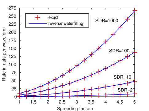
Figure 5: Exact values and reverse waterfilling approximation of the rate for the nonstationary source of Example 3

VI-B2 Comparison with classical work

In Theorem 3, Eqs. (46), (47) may also be used for a parametric representation of the rate distortion function $R(D)$. In parametric form, $R(D)$ has been given by Berger [9] for a broad class of stationary random processes. In the latter parametric interpretation, Eq. (46) is in perfect analogy to [9, Eq. (4.5.52)] [with the (principal term of) WVS instead of the PSD], likewise Eq. (47) with regard to [9, Eq. (4.5.51)] (apart from a factor $\frac{1}{2\pi}$).

VII A Lower Bound for the Spreading Factor

Until now there has been no indication on how large the spreading factor $r$ should at least be chosen so that the dotted equations in the above waterfilling theorems yield useful approximations. The purpose of the present section is to identify a presumed lower bound for $r$.

For any $r\geq 1$ define the operator $\boldsymbol{\hat{A}}(r):L^{2}(\mathbb{R})\rightarrow L^{2}(\mathbb{R})$ by the Weyl symbol $\sigma_{\boldsymbol{\hat{A}}(r)}(x,\xi)=2\pi\rho(r,x,\xi)$, where

$$\rho(r,x,\xi)=\frac{\sigma_{\boldsymbol{\tilde{A}}(r)}(x,\xi)}{\iint\sigma_{\boldsymbol{\tilde{A}}(r)}(x^{\prime},\xi^{\prime})\,\mathrm{d}x^{\prime}\,\mathrm{d}\xi^{\prime}}\,.$$ (53)

Then $\boldsymbol{\hat{A}}(r)$ is self-adjoint, positive, of trace class with the trace $\mathrm{tr}\,\boldsymbol{\hat{A}}(r)=\iint\rho(r,x,\xi)\,\mathrm{d}x\,\mathrm{d}\xi=1$. Thus, $\boldsymbol{\hat{A}}(r)$ is a density operator and the Robertson–Schrödinger uncertainty inequality (RSUI) applies [16]; it reads: For any density operator on $L^{2}(\mathbb{R})$ with a Weyl symbol of the form $2\pi\rho(x,\xi)$, define the moments (for convenience, put $x_{1}=x$, $x_{2}=\xi$)

$$\mu_{i}=\iint x_{i}\rho(x_{1},x_{2})\,\mathrm{d}x_{1}\,\mathrm{d}x_{2},$$ (54)

$$\sigma_{ij}=\iint(x_{i}-\mu_{i})(x_{j}-\mu_{j})\rho(x_{1},x_{2})\,\mathrm{d}x_{1}\,\mathrm{d}x_{2}$$ (55)

and write $\sigma_{i}^{2}=\sigma_{ii},\,i,j=1,2.$ Then it holds

$$\sigma_{1}^{2}\sigma_{2}^{2}\geq\sigma_{12}^{2}+\frac{\hbar^{2}}{4},$$ (56)

where $\hbar$ is the reduced Planck constant (which in our context is always set to one).

Now replace $\rho(x,\xi)$ with $\rho(r,x,\xi)$; since $\rho(r,x,\xi)$ depends on $r$, we shall write $\mu_{i}(r),\,\sigma_{i}^{2}(r),\,\sigma_{ij}(r)$ for its moments (54), (55). Although $\rho(r,x,\xi)$ is not a true probability density function (PDF), since it may assume negative values, its covariance matrix

$$\Sigma(r)=\left(\begin{array}[]{cc}\sigma_{1}^{2}(r)&\sigma_{12}(r)\\ \sigma_{12}(r)&\sigma_{2}^{2}(r)\end{array}\right)$$

is always positive definite (as is the covariance matrix of any density operator [35]). The operators $\boldsymbol{P}_{r},r\geq 1,$ may also be viewed as time–frequency localization operators (TFLOs), comprising in part the TFLOs introduced by Daubechies [11]. Since $\rho(r,t,\omega)$ is the normalized WVS $\Phi(r,t,\omega)$ discussed in Section VI-A [cf. Eq. (44)], it is natural to define the ellipse of concentration (EoC) of $\boldsymbol{P}_{r}$ as the boundary of the region in phase space described by the inequality

$$\big{(}x-\mu_{1}(r),\,\xi-\mu_{2}(r)\big{)}\,\Sigma(r)^{-1}\!\begin{pmatrix}x-\mu_{1}(r)\\ \xi-\mu_{2}(r)\end{pmatrix}\leq 4$$ (57)

and having the property that the uniform distribution on it has the same first and second moments as the PDF at hand [36]. Since the EoC (57) has the area $A_{\mathrm{c}}=\pi\sqrt{\det(4\Sigma(r))}$, the RSUI can now be recast in the inequality $A_{\mathrm{c}}=4\pi\sqrt{\det\Sigma(r)}\geq 4\pi\sqrt{\hbar^{2}/4}=2\pi$, or phrased in words: The area of the EoC of operator $\boldsymbol{P}_{r},r\geq 1,$ is at least $2\pi$.

However, this is not a useful criterion since it holds for any $r$; to get a useful criterion, consider the (true) PDF

$$\rho_{r}(x,\xi)\triangleq\frac{|p_{r}(x,\xi)|^{2}}{\iint|p_{r}(x^{\prime},\xi^{\prime})|^{2}\,\mathrm{d}x^{\prime}\mathrm{d}\xi^{\prime}},$$ (58)

i.e., the normalized principal symbol of $\boldsymbol{\tilde{A}}(r)$ [or $\boldsymbol{A}(r)$]. Note that the denominators in (53) and (58) coincide,

$$\iint\sigma_{\boldsymbol{\tilde{A}}(r)}(x,\xi)\,\mathrm{d}x\,\mathrm{d}\xi=\iint|p_{r}(x,\xi)|^{2}\,\mathrm{d}x\,\mathrm{d}\xi,$$

which is a simple consequence of Eq. (7) (in terms of $\boldsymbol{\tilde{A}}$), Eq. (10) and a generalization to $r\geq 1$; moreover, due to Lemma 1 it holds that

$$\sigma_{\boldsymbol{\tilde{A}}(r)}(x,\xi)=|p_{r}(x,\xi)|^{2}+r^{-2}R_{1}(r,x/r,\xi/r).$$ (59)

The rationale is now as follows: When $r$ is large, $\rho_{r}(x,\xi)$ will be “close to” $\rho(r,x,\xi)$; then the RSUI (56) for $\rho(r,x,\xi)$ may be transposed to $\rho_{r}(x,\xi)$, resulting in a constraint on $r$. With this in mind, replace in (54), (55) function $\rho(x_{1},x_{2})$ with $\rho_{1}(x_{1},x_{2})$ and denote the new values for $\mu_{i},\,\sigma_{i}^{2},\,\sigma_{ij}$ by $m_{i},\,s_{i}^{2},\,s_{ij}$, respectively. By means of Eq. (59) and observing that the common denominator in (53), (58) evaluates to $2\pi c_{p}r^{2}$, we then obtain $\mu_{i}(r)=m_{i}r+o(1)$ and by this $\sigma_{ij}(r)=s_{ij}r^{2}+o(r)$. Plugging the latter in the RSUI (56) for $\rho(r,x,\xi)$ finally results in the desired constraint

$$r^{2}\geq\frac{1}{2\sqrt{s_{1}^{2}s_{2}^{2}-s_{12}^{2}}}+o(1).$$ (60)

Ineq. (60) suggests a lower bound for the spreading factor $r$, thus providing the wanted criterion (in practice, the error term would be neglected). Note that asymptotically, i.e., as $r\rightarrow\infty$, Ineq. (60) (with vanishing error term) becomes a necessary condition.

Example 4

Consider the HS operator $\boldsymbol{P}$ on $L^{2}(\mathbb{R})$ with the Weyl symbol $p\in\mathscr{S}(\mathbb{R}^{2})$ as given in Eq. (35) of Example 1 for any fixed parameter $\gamma>0$. Then the Weyl symbol $p_{r}$ of operator $\boldsymbol{P}_{r},r\geq 1,$ satisfies $\iint|p_{r}(x,\xi)|^{2}\,\mathrm{d}x\,\mathrm{d}\xi=\pi r^{2}$, so that the PDF (58) becomes

$$\rho_{r}(x,\xi)=\frac{1}{\pi r^{2}}\,\mathrm{e}^{-\frac{1}{r^{2}}(\gamma^{-2}x^{2}+\gamma^{2}\xi^{2})}.$$ (61)

An evaluation of the integrals in (54), (55) yields $m_{1}=m_{2}=0,$ $s_{1}^{2}=\gamma^{2}/2,\,s_{2}^{2}=\gamma^{-2}/2$ and $s_{12}=s_{21}=0$. Consequently, Ineq. (60) turns into

$$r^{2}\geq 1+o(1),$$

which, neglecting the error term, means no restriction at all. In fact, in Fig. 3 and Fig. 5 the approximation is already acceptable for spreading factors close to one.

Finally, we add the explanation of the parameter $a$ occurring in Example 2 of Section V-B. To this end, we determine the EoC (57) of the above operator $\boldsymbol{P}_{r},\,r\geq 1,$ by the use of the identity $\boldsymbol{P}_{r}=c\,\boldsymbol{P}^{(\gamma)}_{\delta}$ (see Example 1). The Weyl symbol of the operator $\boldsymbol{P}^{(\gamma)}_{\delta}\!\circ(\boldsymbol{P}^{(\gamma)}_{\delta})^{*}=\boldsymbol{P}^{(\gamma)}_{2\delta}$ is given in closed form in [12]. By this means, Eq. (53) readily becomes

$$\rho(r,x,\xi)=\frac{1}{\pi\alpha\beta}\,\exp\left(-\frac{x^{2}}{\alpha^{2}}-\frac{\xi^{2}}{\beta^{2}}\right),$$

where $\alpha=\gamma\sqrt{\coth\delta},\,\beta=\gamma^{-1}\sqrt{\coth\delta}$. The exact EoC of the operator $\boldsymbol{P}_{r}$ is therefore the ellipse in phase space with the semi-axes $a_{\mathrm{x}}=\sqrt{2}\alpha,\,b_{\mathrm{x}}=\sqrt{2}\beta$ and the equation

$$x^{2}/a_{\mathrm{x}}^{2}+\xi^{2}/b_{\mathrm{x}}^{2}=1.$$

From the PDF (61), we obtain asymptotically, i.e., as $r\rightarrow\infty$, the approximate EoC with semi-axes $a=\sqrt{2}r\gamma,\,b=\sqrt{2}r/\gamma$. For instance, in the case of $r=2,\gamma=1/10$ we find the rather good approximations $a=0.2828,\,b=28.28$ (units omitted) of the exact values $a_{\mathrm{x}}=0.2850,\,b_{\mathrm{x}}=28.50$ (which is somewhat surprising since $r=2$ is still small). In Example 2, the foregoing value of $a$ has been used as an estimate of the effective half duration of a pulse.

VIII Conclusion

Waterfilling theorems in the time–frequency plane for the capacity of an LTV channel with an average energy constraint and the rate distortion function for a related nonstationary source with a squared-error distortion constraint have been stated and rigorous proofs have been given. The waterfilling theorem for the LTV channel has been formulated in terms of the reciprocal squared modulus of the spread Weyl symbol of the LTV filter (times a noise figure), whereas in the reverse waterfilling theorem for the nonstationary source simply the squared modulus of the spread Weyl symbol (times a signal figure) has been used. The latter expression has been related to the WVS of the nonstationary source and recognized as its principal term. The LTV filter, initially an arbitrary HS operator, was later restricted to an operator with a Weyl symbol in the Schwartz space of rapidly decreasing functions. This smoothness assumption was a prerequisite for a Szegő theorem upon which the proofs of both waterfilling theorems rested in an essential way. A self-contained proof of the Szegő theorem has been given. The formulas in the waterfilling theorems depend on the spreading factor and are asymptotic in nature. Two examples with a bivariate Gaussian function as the Weyl symbol showed that the waterfilling theorems may perform well even when the spreading factor is close to one. For the general case, based on an uncertainty inequality, a lower bound for the spreading factor has been suggested.

[Proof of Lemma 1] In this appendix, we shall write $\boldsymbol{x}=(x_{1},x_{2})$ etc. for phase space points $(x,\xi)\in\mathbb{R}^{2}$ and $\mathrm{d}\boldsymbol{x}=\mathrm{d}x_{1}\mathrm{d}x_{2}$ etc. for the corresponding differential. Also, we use the notations $\langle\boldsymbol{x}\rangle\triangleq(1+x_{1}^{2}+x_{2}^{2})^{1/2}$, $\Diamond_{\boldsymbol{x}}\triangleq 1-\partial_{x_{1}}^{2}-\partial_{x_{2}}^{2}$ and write $\partial_{\boldsymbol{x}}^{\boldsymbol{\alpha}}=\partial_{x_{1}}^{\alpha_{1}}\partial_{x_{2}}^{\alpha_{2}}$, ${\boldsymbol{x}}^{\boldsymbol{\beta}}=x_{1}^{\beta_{1}}x_{2}^{\beta_{2}}$ with the multi-indices $\boldsymbol{\alpha}=(\alpha_{1},\alpha_{2})$, $\boldsymbol{\beta}=(\beta_{1},\beta_{2})\in\mathbb{N}_{0}^{2}$. The following proof draws on [17], [26].

For any two operators $\boldsymbol{P},\,\boldsymbol{Q}:L^{2}(\mathbb{R})\rightarrow L^{2}(\mathbb{R})$ with the Weyl symbols $p,\,q\in\mathscr{S}(\mathbb{R}^{2})$, resp., the Weyl symbol of the product $\boldsymbol{P}\boldsymbol{Q}$, denoted by $p\,\#\,q$, is given by [17]

$$(p\,\#\,q)(\boldsymbol{z})\\ =\frac{1}{\pi^{2}}\int_{\mathbb{R}^{2}}\int_{\mathbb{R}^{2}}p(\boldsymbol{z}+\boldsymbol{x})q(\boldsymbol{z}+\boldsymbol{y})\mathrm{e}^{2\mathrm{i}\det(\boldsymbol{x};\boldsymbol{y})}\,\mathrm{d}\boldsymbol{x}\,\mathrm{d}\boldsymbol{y},$$ (62)

where $\det(\boldsymbol{x};\boldsymbol{y})=x_{1}y_{2}-x_{2}y_{1}$. Since we need to compute the Weyl symbol $p_{r}\#\,q_{r},\,r\geq 1,$ we change to the more convenient operation $p\,\#_{r}q$ defined by $(p_{r}\#\,q_{r})(\boldsymbol{z})=(p\,\#_{r}q)(\boldsymbol{z}/r)$. A computation yields (see [17] and [26] in the case of $r=1$)

$$(p\,\#_{r}q)(\boldsymbol{z})=\sum_{k=0}^{m-1}r^{-2k}a_{k}(\boldsymbol{z})+r^{-2m}R_{m}(r,\boldsymbol{z})$$

with the functions $a_{k}\in\mathscr{S}(\mathbb{R}^{2})$ given by $a_{k}(\boldsymbol{z})=F_{k}(\boldsymbol{z},\boldsymbol{z})$, and

$$R_{m}(r,\boldsymbol{z})=m\int_{0}^{1}(1-t)^{m-1}\bigg{\{}\frac{1}{\pi^{2}}\int_{\mathbb{R}^{2}}\int_{\mathbb{R}^{2}}\mathrm{e}^{2\mathrm{i}\det(\boldsymbol{x};\boldsymbol{y})}\\ \cdot F_{m}(\boldsymbol{z}+t\boldsymbol{x}/r,\boldsymbol{z}+\boldsymbol{y}/r)\,\mathrm{d}\boldsymbol{x}\,\mathrm{d}\boldsymbol{y}\bigg{\}}\mathrm{d}t,$$ (63)

where

$$F_{k}(\boldsymbol{x},\boldsymbol{y})=\frac{\mathrm{i}^{k}}{k!2^{k}}(\partial_{x_{1}}\partial_{y_{2}}-\partial_{x_{2}}\partial_{y_{1}})^{k}\,[p(\boldsymbol{x})q(\boldsymbol{y})]$$ (64)

for $k=0,\ldots,m$. Note that $a_{0}(\boldsymbol{z})=p(\boldsymbol{z})q(\boldsymbol{z})$.

First, we show that when $a\in\mathscr{S}(\cdot,\mathbb{R}^{2}),\,b\in\mathscr{S}(\mathbb{R}^{2})$, then $c=a\,\#_{r}b\in\mathscr{S}(\cdot,\mathbb{R}^{2}),\,r\geq 1$. To this end, note that for any positive integers $L,\,M$ it holds $\Diamond_{\boldsymbol{y}}^{M}\mathrm{e}^{2\mathrm{i}\det(\boldsymbol{x};\boldsymbol{y})}=\langle 2\boldsymbol{x}\rangle^{2M}\mathrm{e}^{2\mathrm{i}\det(\boldsymbol{x};\boldsymbol{y})}$ and $\Diamond_{\boldsymbol{x}}^{L}\mathrm{e}^{2\mathrm{i}\det(\boldsymbol{x};\boldsymbol{y})}=\langle 2\boldsymbol{y}\rangle^{2L}\mathrm{e}^{2\mathrm{i}\det(\boldsymbol{x};\boldsymbol{y})}$. By partial integration we then obtain from (62) the representation

$$c(r,\boldsymbol{z})=\frac{1}{\pi^{2}}\int_{\mathbb{R}^{2}}\int_{\mathbb{R}^{2}}\mathrm{e}^{2\mathrm{i}\det(\boldsymbol{x};\boldsymbol{y})}\Diamond_{\boldsymbol{x}}^{L}\frac{a(r,\boldsymbol{z}+\boldsymbol{x}/r)}{\langle 2\boldsymbol{x}\rangle^{2M}}\\ \cdot\frac{\Diamond_{\boldsymbol{y}}^{M}[b(\boldsymbol{z}+\boldsymbol{y}/r)]}{\langle 2\boldsymbol{y}\rangle^{2L}}\,\mathrm{d}\boldsymbol{x}\,\mathrm{d}\boldsymbol{y}.$$ (65)

Concerning the computation of $\Diamond_{\boldsymbol{x}}^{L}(\cdot)$ occurring in (65), note that for any $\boldsymbol{\gamma}=(\gamma_{1},\gamma_{2})\in\mathbb{N}_{0}^{2},\,0\leq\gamma_{1}+\gamma_{2}\leq 2L,$ it holds

$$|\partial_{\boldsymbol{x}}^{\boldsymbol{\gamma}}[\langle 2\boldsymbol{x}\rangle^{-2M}]|\leq C\langle 2\boldsymbol{x}\rangle^{-2M},\boldsymbol{x}\in\mathbb{R}^{2},$$

where $C=C(M,L)<\infty$. Consequently, for any $\boldsymbol{\alpha},\boldsymbol{\beta}\in\mathbb{N}_{0}^{2}$, the expression $|\boldsymbol{z}^{\boldsymbol{\beta}}\partial_{\boldsymbol{z}}^{\boldsymbol{\alpha}}c(r,\boldsymbol{z})|$ may be upper bounded for all $\boldsymbol{z}\in\mathbb{R}^{2}$ and $r\geq 1$ by a linear combination (with positive coefficients effectively not depending on $r$ since $1/r\leq 1$) of terms of the form

$$\int_{\mathbb{R}^{2}}\int_{\mathbb{R}^{2}}\frac{|a_{\lambda}(r,\boldsymbol{z}+\boldsymbol{x}/r)b_{\mu}(\boldsymbol{z}+\boldsymbol{y}/r)|}{\langle 2\boldsymbol{x}\rangle^{2M}\langle 2\boldsymbol{y}\rangle^{2L^{\prime}}}\,\mathrm{d}\boldsymbol{x}\,\mathrm{d}\boldsymbol{y},$$ (66)

where $a_{\lambda}\in\mathscr{S}(\cdot,\mathbb{R}^{2})$, $b_{\mu}\in\mathscr{S}(\mathbb{R}^{2})$ and $M\geq 2$, $2\leq L^{\prime}\leq L$ ($L$ sufficiently large). Here we have used, possibly repeatedly, the fact that when $b_{\mu}\in\mathscr{S}(\mathbb{R}^{2}),$ then $z_{i}b_{\mu}(\boldsymbol{z}+\boldsymbol{y}/r)=\tilde{b}_{\mu}(\boldsymbol{z}+\boldsymbol{y}/r)-(y_{i}/r)b_{\mu}(\boldsymbol{z}+\boldsymbol{y}/r)$ where $\tilde{b}_{\mu}$ defined by $\tilde{b}_{\mu}(\boldsymbol{z})=z_{i}b_{\mu}(\boldsymbol{z})$ is again in $\mathscr{S}(\mathbb{R}^{2})$. Replace the numerator of the integrand in (66) by a constant upper bound and integrate. Summing up, we obtain the inequality

$$|\boldsymbol{z}^{\boldsymbol{\beta}}\partial_{\boldsymbol{z}}^{\boldsymbol{\alpha}}c(r,\boldsymbol{z})|\leq C_{\boldsymbol{\alpha}\boldsymbol{\beta}}<\infty,\,\boldsymbol{z}\in\mathbb{R}^{2},$$ (67)

where the constant $C_{\boldsymbol{\alpha}\boldsymbol{\beta}}$ does not depend on $r\geq 1$.

Second, we show that $R_{m}\in\mathscr{S}(\cdot,\mathbb{R}^{2})$. The integral $I(t,r,\boldsymbol{z})$ between braces $\{\ldots\}$ in (63) is a linear combination of expressions on the right-hand side of Eq. (65) after the substitution $a(r,\boldsymbol{z}+\boldsymbol{x}/r)\leftarrow(\partial_{\boldsymbol{x}}^{\boldsymbol{\alpha}}p)(\boldsymbol{z}+t\boldsymbol{x}/r)$ and $b(\boldsymbol{z}+\boldsymbol{x}/r)\leftarrow(\partial_{\boldsymbol{x}}^{\boldsymbol{\beta}}q)(\boldsymbol{z}+\boldsymbol{x}/r)$, the partial derivatives (of order $m$) coming from those in (64). Now let $\alpha,\beta\in\mathbb{N}_{0}^{2}$ be arbitrary. By the same reasoning as before, we infer that $|\boldsymbol{z}^{\boldsymbol{\beta}}\partial_{\boldsymbol{z}}^{\boldsymbol{\alpha}}I(t,r,\boldsymbol{z})|$ may be upper bounded by a linear combination (with positive coefficients effectively not depending on $r$ and $t$ since $t/r\leq 1$) of terms analogous to (66). Taking the supremum of the numerators of the integrands, we get rid of the variable $t$ so that the integral with respect to $t$ occurring in (63) may be computed (evaluating to 1). Again summing up, we obtain the analog to Ineq. (67), where $c(r,\boldsymbol{z})$ is to be replaced with $R_{m}(r,\boldsymbol{z})$.

Now we are in a position to prove Eq. (15). Take any function $b\in\mathscr{S}(\mathbb{R}^{2})$. Then

$$((p\,\#_{r}q)\,\#_{r}b)(\boldsymbol{z})=\sum_{k=0}^{m-1}r^{-2k}(a_{k}\,\#_{r}b)(\boldsymbol{z})\\ +r^{-2m}R_{m,0}(r,\boldsymbol{z}),$$

where $R_{m,0}=R_{m}\,\#_{r}b\in\mathscr{S}(\cdot,\mathbb{R}^{2})$ and

$$(a_{k}\,\#_{r}b)(\boldsymbol{z})=\sum_{j=0}^{m-k-1}r^{-2j}a_{kj}(\boldsymbol{z})+r^{-2(m-k)}R_{k,m-k}(r,\boldsymbol{z})$$

with the functions $a_{kj}\in\mathscr{S}(\mathbb{R}^{2})$ and $R_{k,m-k}\in\mathscr{S}(\cdot,\mathbb{R}^{2}),$ $k=0,\ldots,m-1$. One readily finds

$$((p\,\#_{r}q)\,\#_{r}b)(\boldsymbol{z})=\sum_{k=0}^{m-1}r^{-2k}\tilde{a}_{k}(\boldsymbol{z})+r^{-2m}\tilde{R}_{m}(r,\boldsymbol{z}),$$

where the functions $\tilde{a}_{k}\in\mathscr{S}(\mathbb{R}^{2})$ and $\tilde{R}_{m}\in\mathscr{S}(\cdot,\mathbb{R}^{2})$ are given by

$$\tilde{a}_{k}(\boldsymbol{z})=\sum_{i+j=k\atop i,j\geq 0}a_{ij}(\boldsymbol{z}),\,\tilde{R}_{m}(r,\boldsymbol{z})=\sum_{k=0}^{m}R_{k,m-k}(r,\boldsymbol{z}).$$

Note that $\tilde{a}_{0}=pqb$. Putting $q=\bar{p}$ and alternately $b=p$ or $b=\bar{p}$ we obtain by induction, observing that brackets may be omitted, for the Weyl symbol $\sigma_{\boldsymbol{A}^{n}(r)}(\boldsymbol{z})$ of $\boldsymbol{A}^{n}(r)$,

$$\underbrace{(p_{r}\#\,\bar{p}_{r}\#\ldots\#\,p_{r}\#\,\bar{p}_{r})}_{\displaystyle n\;\mbox{factors}\;p_{r}\#\,\bar{p}_{r}}(\boldsymbol{z})=(p\,\#_{r}\bar{p}\,\#_{r}\ldots\#_{r}p\,\#_{r}\bar{p})(\boldsymbol{z}/r),$$

the asymptotic expansion as given in Eq. (15) [written without superscripts $\tilde{}$ again and after the substitution $\boldsymbol{z}\leftarrow(x,\xi)$].

References

• [1] C. E. Shannon, “Communication in the presence of noise,” Proc. IRE, vol. 37, pp. 10–21, 1949.
• [2] R. G. Gallager, Information Theory and Reliable Communication. New York, NY: Wiley, 1968.
• [3] S. Barbarossa and A. Scaglione, “On the capacity of linear time-varying channels,” Proc. IEEE Int. Conf. Acustics Speech Signal Process., 1999, vol. 5, pp. 2627–2630.
• [4] P. Jung, “On the Szegö-asymptotics for doubly-dispersive Gaussian channels,” Proc. IEEE Int. Symp. Inf. Theory, St. Petersburg, Russia, 2011, pp. 2852–2856.
• [5] B. Farrell and T. Strohmer, “Eigenvalue estimates and mutual Information for the linear time-varying channel,” IEEE Trans. Inf. Theory, vol. 57, pp. 5710–5718, 2011.
• [6] G. Durisi, U. G. Schuster, H. Bölcskei, and S. Shamai (Shitz), “Noncoherent capacity of underspread fading channels,” IEEE Trans. Inf. Theory, vol. 56, pp. 367–395, 2010.
• [7] P. A. Bello, “Characterization of randomly time-variant linear channels,” IEEE Trans. Commun. Syst., vol. 11, pp. 360–393, 1963.
• [8] A. N. Kolmogorov, “On the Shannon theory of information transmission in the case of continuous signals,” IRE Trans. Inf. Theory, vol. 2, pp. 102–108, 1956.
• [9] T. Berger, Rate Distortion Theory: A Mathematical Basis for Data Compression. Englewood Cliffs, NJ: Prentice-Hall, 1971.
• [10] A. Kipnis and A. J. Goldsmith, “Distortion rate function of cyclo-stationary Gaussian processes,” Proc. IEEE Int. Symp. Inf. Theory, Honolulu, HI, 2014, pp. 2834–2838.
• [11] I. Daubechies, “Time-frequency localization operators: A geometric phase space approach,” IEEE Trans. Inf. Theory, vol. 34, pp. 605–612, 1988.
• [12] E. Hammerich, “Waterfilling theorems in the time-frequency plane for the heat channel and a related source,” Proc. IEEE Int. Symp. Inf. Theory, Honolulu, HI, 2014, pp. 2416–2420.
• [13] M. Reed and B. Simon, Methods of Modern Mathematical Physics I: Functional Analysis. New York, NY: Academic Press, 1972.
• [14] J. C. T. Pool, “Mathematical aspects of the Weyl correspondence,” J. Math. Phys, vol. 7, pp. 66–76, 1966.
• [15] W. Kozek and F. Hlawatsch, “Time-frequency representation of linear time-varying systems using the Weyl symbol,” IEE Sixth Int. Conf. Digital Signal Process. Commun., Loughborough, UK, 1991, pp. 25–30.
• [16] M. A. de Gosson, Symplectic Methods in Harmonic Analysis and in Mathematical Physics. Basel: Birkhäuser, 2011.
• [17] G. B. Folland, Harmonic Analysis in Phase Space. Princeton, NJ: Princeton University Press, 1989.
• [18] K. Gröchenig, Foundations of Time-Frequency Analysis. Boston: Birkhäuser, 2001.
• [19] G. Matz and F. Hlawatsch, “Time-frequency transfer function calculus (symbolic calculus) of linear time-varying systems (linear operators) based on a generalized underspread theory,” J. Math. Phys., vol. 39, pp. 4041–4070, 1998.
• [20] W. Kozek, “On the transfer function calculus for underspread LTV channels,” IEEE Trans. Signal Process., vol. 45, pp. 219–223, 1997.
• [21] D. Robert, Autour de l’Approximation Semi-Classique. Boston: Birkhäuser, 1987.
• [22] M. A. de Gosson and F. Luef, “Principe d’incertitude et positivité des opérateurs à trace; applications aux opérateurs densité,” Ann. H. Poincaré, vol. 9, pp. 329–346, 2008.
• [23] A. J. E. M. Janssen and S. Zelditch, “Szegö limit theorems for the harmonic oscillator,” Trans. Amer. Math. Soc., vol. 280, pp. 563–587, 1983.
• [24] A. P. Calderón and R. Vaillancourt, “On the boundedness of pseudo-differential operators,” J. Math. Soc. Japan, vol. 23, pp. 374–378, 1971.
• [25] H. Widom, Asymptotic expansions for pseudodifferential operators on bounded domains, vol. 1152 of Lect. Notes Math., Berlin: Springer, 1985.
• [26] J. P. Oldfield, “Two-term Szegő theorem for generalized anti-Wick operators,” 2014 [Online]. Available: arXiv:1404.2256v2
• [27] H. G. Feichtinger and K. Nowak, “A Szegö-type theorem for Gabor-Toeplitz localization operators,” Michigan Math. J., vol. 49, pp. 13–21, 2001.
• [28] E. Hammerich, “A sampling theorem for time-frequency localized signals,” Sampl. Theory Signal Image Process., vol. 3, pp. 45–81, 2004.
• [29] R. M. Corless, G. H. Gonnet, D. E. G. Hare, D. J. Jeffrey, and D. E. Knuth, “On the Lambert W function,” Adv. Computat. Math., vol. 5, pp. 329–359, 1996.
• [30] E. Hammerich, “On the heat channel and its capacity,” Proc. IEEE Int. Symp. Inf. Theory, Seoul, Korea, 2009, pp. 1809–1813.
• [31] T. M. Cover and J. A. Thomas, Elements of Information Theory. 2nd ed. Hoboken, NJ: Wiley, 2006.
• [32] P. Flandrin and W. Martin, “The Wigner-Ville spectrum of nonstationary random signals,” in The Wigner Distribution, W. Mecklenbräuker and F. Hlawatsch, Eds.    Amsterdam: Elsevier, 1997, pp. 211–267.
• [33] W. Kozek, “Matched Weyl–Heisenberg expansions of nonstationary environments,” Ph.D. diss., Vienna Univ. Technol., Austria, 1996.
• [34] P. Flandrin, “On the positivity of the Wigner–Ville spectrum,” Signal Process., vol. 11, pp. 187-189, 1986.
• [35] F. J. Narcowich, “Geometry and uncertainty,” J. Math. Phys., vol. 31, pp. 354–364, 1990.
• [36] H. Cramér, Mathematical Methods of Statistics. Princeton, NJ: Princeton Univ. Press, 1946.