A disk wind interpretation of the strong Fe K$\alpha$ features in 1H 0707-495

Abstract

1H 0707-495 is the most convincing example of a supermassive black hole with an X-ray spectrum being dominated by extremely smeared, relativistic reflection, with the additional requirement of strongly supersoler iron abundance. However, here we show that the iron features in its 2–10 keV spectrum are rather similar to the archetypal wind dominated source, PDS 456. We fit all the 2–10 keV spectra from 1H 0707-495 using the same wind model as used for PDS 456, but viewed at higher inclination so that the iron absorption line is broader but not so blueshifted. This gives a good overall fit to the data from 1H 0707-495, and an extrapolation of this model to higher energies also gives a good match to the NuSTAR data. Small remaining residuals indicate that the iron line emission is stronger than in PDS 456. This is consistent with the wider angle wind expected from a continuum driven wind from the super-Eddington mass accretion rate in 1H 0707-495, and/or the presence of residual reflection from the underlying disk though the presence of the absorption line in the model removes the requirement for highly relativistic smearing, and highly supersoler iron abundance. We suggest that the spectrum of 1H 0707-495 is sculpted more by absorption in a wind than by extreme relativistic effects in strong gravity.

1 Introduction

1H 0707-495 (hereafter 1H0707) is a Narrow Line Seyfert 1 (NLS1) galaxy i.e. a low mass, high mass accretion rate (in terms of Eddington) AGN (Boroson, 2002). It shows extreme dips in its X-ray lightcurve, during which the spectra have a steep drop around 7 keV, associated with iron K$\alpha$ (Boller et al., 2002). These spectra are generally fit with ionized reflection, but the features are so strong and broad that this interpretation requires extreme conditions. The requirements are that the black hole spin is close to maximal, that the incident radiation is strongly focussed onto the inner edge of the disk whilst being suppressed in the direction of the observer, and that iron is overabundant by a factor of 7–20 (Fabian et al., 2004; Fabian et al., 2009, 2012; Zoghbi et al., 2010). The first two features can be explained together in a model where the dips are caused by an extremely compact X-ray source on the spin axis of the black hole approaching the event horizon (hereafter the lamppost model). The resulting strong light bending focusses the intrinsic continuum away from the observer (producing the drop in flux), whilst simultaneously strongly illuminating the very inner disk (Miniutti & Fabian, 2004).

However, the optical/UV continuum from 1H0707 implies that the black hole is accreting at a super-Eddington rate (Done & Jin, 2016). Hence the inner disk is unlikely to be flat, as assumed in the lamppost reflection models, and should launch a strong wind due to continuum radiation pressure (Ohsuga & Mineshige, 2011; Jiang et al., 2014; Sa̧dowski & Narayan, 2016; Hashizume et al., 2015). Thus this source, and other NLS1s with similarly very high mass accretion rates and similarly extreme X-ray spectra (e.g. IRAS 13224-3809: Ponti et al., 2010) may have spectral features which are affected by absorption and/or emission/scattering in a wind. Absorption has been persistently suggested as an alternative explanation for the features seen around iron in the NLS1s, though the spectra are complex and not easy to fit (Mkn 766: Miller et al. 2007; Turner et al. 2007, MCG-6-30-15: Inoue & Matsumoto 2001; Gallo et al. 2004; Miller et al. 2008, 1H0707: Boller et al. 2002; Miller et al. 2010; Mizumoto et al. 2014).

The recent discovery of blueshifted ($v>10000$ km s^-1 i.e. $0.03c$), narrow absorption lines from very highly ionized material (mostly He- and H-like Fe K$\alpha$) has focussed attention on winds from the inner disk. These Ultra-Fast Outflows (UFOs) are seen from a variety of nearby Seyfert galaxies (see e.g. the compilation by Tombesi et al., 2010). The fast velocities imply that the winds are launched from the inner disk since winds typically have terminal velocities similar to the escape velocity from their launch radius. However, the launch mechanism is not well understood (e.g. Tombesi et al., 2012). Standard broad line Seyfert galaxies are well below their Eddington limit, so that they cannot power winds from continuum radiation pressure alone. Moreover, they have strong X-ray emission which ionizes the disk material above where it has substantial UV opacity, suppressing a UV line driven disk wind (Proga et al., 2000; Proga & Kallman, 2004; Higginbottom et al., 2014). Magnetic driving seems the only remaining mechanism, but this depends strongly on the (unknown) magnetic field configuration so is not yet predictive (Proga, 2003).

Despite this general lack of understanding of the origin of the winds, the fastest, $v>0.2c$, and most powerful UFOs are seen in luminous quasars such as PDS 456 (Reeves et al., 2009; Nardini et al., 2015) and APM 08279+5255, a high redshift quasar which is gravitationally lensed (Chartas et al., 2002). These AGN are not standard broad line Seyfert galaxies. Instead, since both quasars are around the Eddington limit, they could power a continuum driven wind. Also, black holes in both quasars are very high mass ($\sim 10^{9}-10^{10}$ M_⊙) so that their accretion disk spectra should peak in the UV. PDS 456 is also clearly intrinsically X-ray weak (Hagino et al., 2015), and APM 08279+5255 may also be similar (Hagino et al, in preparation). A more favorable set of circumstances for UV line driving is hard to imagine. Nonetheless, the extremely high ionization of the UFO in PDS 456 means that the observed wind material has no UV opacity, so UV line driving must take place out of the line of sight if this mechanism is important (Hagino et al., 2015).

Whatever the launch mechanism, PDS 456 clearly has features at Fe K$\alpha$ which are dominated by a wind from the inner disk rather than extreme reflection from the inner disk (Reeves et al., 2003, 2009; Nardini et al., 2015). The best wind models so far use Monte-Carlo techniques to track the complex, geometry and velocity dependent, processes in the wind including absorption, emission, continuum scattering and resonance line scattering (Sim et al., 2008, 2010; Hagino et al., 2015). While these models have been used to fit Mkn 766 (Sim et al., 2008), PG 1211+143 (Sim et al., 2010), PDS 456 (Hagino et al., 2015), and six other ‘bare’ Seyfert 1 nuclei (Tatum et al., 2012), they have not yet been applied to 1H0707, the object with the strongest and broadest iron features, and the one where the reflection models require the most extreme conditions (Fabian et al., 2009, 2012). Previous work showed that simple wind models, where the iron features were described using a single P Cygni profile, can fit the deep drop at $\sim 7$ keV seen in one observation of this object (Done et al., 2007), but here we use the full Monte-Carlo wind code, monaco, of Hagino et al. (2015) to see if this can adequately fit all the multiple observations of 1H0707. We show that inner disk wind models can indeed give a good overall description of the 2–10 keV spectra, and that extrapolating these to higher energies can also match the NuSTAR data from this source.

2 Observations of 1H0707 and comparison to the archetypical wind source PDS 456

Table 1: XMM-Newton and Suzaku observations of 1H0707

Name	Obs ID	Start Date	Net exposure (ks)
XMM-Newton
Obs1	0110890201	2000-10-21	37.8
Obs2	0148010301	2002-10-13	68.1
Obs3	0506200301	2007-05-14	35.8
Obs4	0506200201	2007-05-16	26.9
Obs5	0506200501	2007-06-20	32.6
Obs6	0506200401	2007-07-06	14.7
Obs7	0511580101	2008-01-29	99.6
Obs8	0511580201	2008-01-31	66.4
Obs9	0511580301	2008-02-02	59.8
Obs10	0511580401	2008-02-04	66.6
Obs11	0653510301	2010-09-13	103.7
Obs12	0653510401	2010-09-15	102.1
Obs13	0653510501	2010-09-17	95.8
Obs14	0653510601	2010-09-19	97.7
Obs15	0554710801	2011-01-12	64.5
Suzaku
SuzakuObs	700008010	2005-12-03	97.9/100.4/97.2/97.8

¹ Net exposure time of pn for XMM-Newton and XIS0/XIS1/XIS2/XIS3 for Suzaku, respectively.

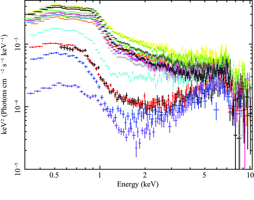
Figure 1: All 2–10 keV spectra observed by XMM-Newton/pn and Suzaku/FI detectors, unfolded against a $\Gamma=2$ power law.

1H0707 was observed by Suzaku and XMM-Newton for many times as listed in Tab. 1. We reduce both XMM-Newton pn and Suzaku XIS data with standard screening conditions: ${\rm PATTERN}\leq 4$ events for XMM-Newton/pn data and grade 0, 2, 3, 4 and 6 events for Suzaku/XIS data were used. Bad time intervals were also excluded. XMM-Newton data in time intervals when background rates of ${\rm PATTERN}=0$ events at energy $>10$ keV exceeded 0.4 counts s^-1 were removed. Suzaku data within 436 s of passage through the South Atlantic Anomaly (SAA), and within an Earth elevation angle (ELV) $<5^{\circ}$ and Earth day-time elevation angles (DYE_ELV) $<20^{\circ}$ were excluded. Spectra were extracted from circular regions of 64$\arcsec$ and 2.$\arcmin$9 diameter for XMM-Newton and Suzaku, respectively. Background spectra of XMM-Newton data were extracted from circular regions of the same diameter in the same chip as the source regions, while background spectra of Suzaku data were extracted from annular region from 7.$\arcmin$0 to 14.$\arcmin$0 diameter. The observed data show a large variability in continuum spectra as seen in Fig. 1. There is an obvious variability in the 2–6 keV continuum shape and in the strength of the iron K features around 7 keV.

Figure 2 shows brightest and faintest 2–12 keV (rest frame) spectra seen in PDS 456, the archetypal inner disk wind source, (black/grey: ObsID 707035030/701056010), together with the corresponding brightest/faintest observations of 1H0707 (cyan/blue: Obs12/Obs15). The spectra are similarly harder when fainter, and show a similarly deep drop at iron K. In PDS 456, these features are all generally associated with absorption, with the deep drop at iron K interpreted as Fe K$\alpha$ absorption lines from highly ionized material in the wind, while the variability at lower energies can be described by complex absorption from lower ionization material (Reeves et al., 2003, 2009; Nardini et al., 2015; Hagino et al., 2015). Conversely, the spectral features in 1H0707 are generally associated with extreme relativistic reflection, especially in the hardest/dimmest spectra (Fabian et al., 2009, 2012). Nonetheless, the 2–10 keV spectra of 1H0707 and PDS 456 are quite similar, both in range of continuum shapes and in the shape of the drop around Fe K$\alpha$.

However, there are also some more subtle differences. The sharp drop in 1H0707 is at $\sim 7.0\textrm{--}7.5$ keV, whereas it is at $8.5\textrm{--}9.0$ keV in PDS 456, and the recovery of the continuum after the absorption lines at higher energies is more evident in PDS 456 than in 1H0707. Thus if these features are from a wind in 1H0707, it shares many similarities with the wind in PDS 456 but cannot have exactly the same parameters.

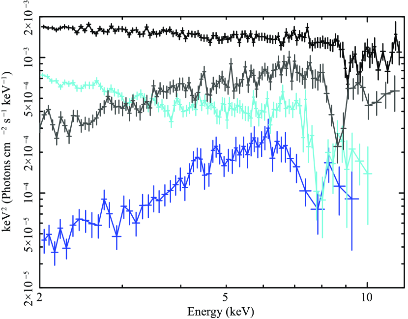
Figure 2: Comparison between the brightest/faintest spectra of PDS 456 (black/grey: ObsID 707035030/701056010) and the brightest/faintest spectra of 1H0707 (cyan/blue: Obs12/Obs15). The 2–10 keV spectra show a similar range in 2-5 keV spectral slope, and similarly deep features at Fe K$\alpha$, though these start at a lower energy in 1H0707, and are broader than in PDS 456.

3 The monaco simulations for PDS 456

The wind in PDS 456 was modeled by using the monaco Monte-Carlo code. This wind model and the calculation scheme are fully described in Hagino et al. (2015), and the general framework design of the code is described in Odaka et al. (2011). To summarize its main features, it follows Sim et al. (2010) and assumes a biconical wind geometry, where the wind is launched from radii $R_{\rm min}$ to $R_{\rm max}$ along streamlines which diverge from a focal point at a distance $d$ below the black hole. The radial velocity of material along each streamline of length $l$ from its launch point on the disk is

$$v_{\rm r}(l)=v_{0}+(v_{\infty}-v_{0})\left(1-\frac{R_{\rm min}}{R_{\rm min}+l}\right)^{\beta},$$ (1)

while the azimuthal velocity is assumed to be Keplarian at the launch point, and then conserves angular momentum as the wind expands. We assume $v_{0}$ is negligible. There can also be a turbulent velocity, $v_{\rm t}$.

The total wind mass loss rate $\dot{M}_{\rm wind}$ is given as

$$\dot{M}_{\rm wind}=1.23m_{\rm p}n(r)v_{\rm r}(r)4\pi D^{2}\frac{\Omega}{4\pi},$$ (2)

which sets the density $n(r)$ as a function of radius in the wind. Here, $1.23m_{\rm p}$, $D$ and $\Omega$ are an ion mass, the distance from the focal point and a solid angle of the wind, respectively. The bicone is split into 100 radial shells, and the ion populations are calculated in each shell by using the xstar photoionization code on the assumption that the central source is a power law spectrum with photon index $\Gamma$ and ionizing luminosity $L_{\rm x}$ (adjusted for special relativistic dimming from the radial outflow velocity). The resulting H- and He-like ion densities of each element are put in the Monte-Carlo radiation transfer simulator monaco, which uses the Geant4 toolkit library (Allison et al., 2006) for photon tracking, but extended to include a full treatment of photon processes related to H- and He-like ions (Watanabe et al., 2006).

Thus there are 9 major free parameters. $R_{\rm min}$, $R_{\rm max}$ and $d$ determine the geometry. $v_{\infty}$, $v_{\rm t}$ and $\beta$ define the radial velocity structure. These geometry and velocity structure together with $\dot{M}_{\rm wind}$ determine the density structure, which then sets the ionization state given $L_{\rm x}$ and $\Gamma$.

This wind model is self-similar in ionization structure and column density for systems at different mass but the same Eddington ratio $\dot{m}=L_{\rm bol}/L_{\rm Edd}$ i.e. the same geometry, velocity structure and spectral index. The ionization state $\xi=L_{\rm x}/nD^{2}$ can be written as

$$\xi=1.23m_{\rm p}v_{\rm r}\Omega L_{\rm x}/\dot{M}_{\rm wind},$$ (3)

where equation 2 is used. Since the ionizing luminosity can be written as $L_{\rm x}=f_{\rm x}\dot{m}\eta\dot{M}_{\rm Edd}c^{2}$ where $f_{\rm x}=L_{\rm x}/L_{\rm bol}$, then the ionization parameter reads

$$\xi=1.23m_{\rm p}v_{\rm r}\Omega f_{\rm x}\dot{m}\eta c^{2}/(\dot{M}_{\rm wind}/\dot{M}_{\rm Edd}).$$ (4)

Thus the ionization state of the wind is determined by $\dot{M}_{\rm wind}/\dot{M}_{\rm Edd}$, and not by black hole mass directly.

The observed spectral properties strongly depend on the inclination angle. The energy at which the line absorption is seen depends on both the terminal wind speed and the inclination angle at which we see the wind, whereas the width of the absorption line depends on the spread of velocities along the line of sight. This spread in turn depends on the terminal velocity of the wind, how much of the acceleration region is along the line of sight, and the projected angle between the wind streamlines and the line of sight. Along the bicone, a fast wind acceleration law means that most of the wind is at its terminal velocity. Thus the line width is fairly small and the blueshift indicates the true wind velocity. At higher inclination angles, the line of sight cuts across the acceleration region so the absorption line is wider and the total blueshift is not so large since the line of sight includes much lower velocity material. Thus the same wind seen at different line of sight can have very different properties in terms of the measured width and blueshift of the absorption line.

We illustrate this inclination dependence in Fig. 3 by showing the monaco wind model for PDS 456 at a larger range of inclination angles than in Hagino et al. (2015). This wind model has $R_{\rm min}=d=20R_{\rm g}$ and $R_{\rm max}=1.5R_{\rm min}$ so that the wind fills a bicone between $\theta_{\rm min}=45^{\circ}$ to $\theta_{\rm max}=56^{\circ}.3$, i.e. the wind fills a solid angle $\Omega/4\pi=0.15$. We fix the velocity law at $\beta=1$ and assume $v_{0}=v_{\rm t}=10,000$ km/s. The terminal velocity is set at $v_{\infty}=-0.3c$, which is consistent with the escape velocity from $R_{\rm min}$. The mass outflow rate is $\dot{M}_{\rm wind}/\dot{M}_{\rm Edd}=0.3$, and the ionizing spectrum with $L_{\rm x}/L_{\rm Edd}=10^{44}/10^{47}$ and $\Gamma=2.5$ is assumed. It is clear that inclination angles larger than $\theta_{\rm max}$ gives a line which is less blueshifted, but broader, as required to fit 1H0707. The width is accentuated because the larger column density of the wind means that the ionized iron edge is also important in absorbing the spectrum blueward of the absorption line. These high inclination monaco model spectra for PDS 456 give iron K features which are quite similar to those required for 1H0707.

Figure 3: monaco wind model for PDS 456 seen at different inclination angles. The direct and reprocessed components are plotted in red and blue, respectively. The sums of these components are plotted in black. Angles from $45-47^{\circ}$ intercept only the top of the bicone. Almost all the wind is at the terminal velocity of $0.3c$ so the lines are strongly blueshifted, but fairly narrow. Larger angles cut through more of the wind, so the lines are deeper, and intersect progressively more of the acceleration zone, so the lines are broader and blend into each other. Angles larger than $56.6^{\circ}$ now cut across the bicone, so the lines are less blueshifted, but include even more of the acceleration zone, so the lines are broader, and now the wind is close to optically thick so the edge is also important. Thus the line absorption shifts from two obviously narrow lines which are strongly blueshifted, to a single, very broad absorption line which is not strongly blueshifted.

4 Fitting the range of 2–10 keV data from 1H0707

4.1 Tailoring the wind model to 1H0707

We first see whether the monaco model calculations for the archetypal wind source PDS 456 can fit the features seen in 1H0707 by simply viewing the wind at a larger inclination angle. We fit to Obs12, which is the steepest spectrum seen from 1H0707. We assume that this steepest spectrum has negligible absorption from lower ionization species. We use the monaco results from PDS 456, as coded into a multiplicative model by Hagino et al. (2015), on a power law continuum. Free parameters are the inclination and the redshift. By allowing the redshift to be free, we are able to fit for a slightly different wind velocity. This fitting gives ${\chi_{\nu}}^{2}=133/87$ for a power law index of $2.65\pm 0.05$ (see Fig. 4a and Table 2).

We compare this model with the standard extreme reflection interpretation. We use the ionized reflection atable models reflionx (Ross & Fabian, 2005), and convolve these with kdblur, allowing the emissivity index, inner disk radius, inclination angle, iron abundance and ionization parameter to be free parameters. This gives ${\chi_{\nu}}^{2}=115/83$ for $\Gamma=3.07\pm 0.15$, a somewhat better fit, but with more free parameters (Fig. 4b). Inspection of the residuals shows that the wind model underpredicts the emission line flux, whereas the reflection model underpredicts the extent of the drop at $\sim 7.5$ keV. This suggests that the drop is better matched by the wind, but there is more line emission than predicted in the PDS 456 models.

This discrepancy could be produced by the wind itself. A wider angle wind will intercept more of the source luminosity, and have stronger emission/reflection/scattering features at iron K for a given absorption line strength. We will investigate such wide angle winds in a subsequent paper. Alternatively (or additionally), there can be lower ionization species in the wind which also add to the line emission. We approximate both of these physical pictures by adding a phenomenological broad gaussian line to the wind model, and find a better fit than either reflection or the PDS 456 wind alone (${\chi_{\nu}}^{2}=107/84$: Fig. 4c).

Another possible origin for the excess iron line emission is that there is residual reflection from the underlying disk. We add a phenomenological blurred reflection component as above, allowing the amount of disk reflection, emissivity index, inner disk radius, inclination angle, iron abundance and ionization parameter to be free. This is a better fit than the gaussian line ($\chi^{2}_{\nu}=92.0/82$), mostly because the reflection model also includes hydrogen-like sulphur line emission at 2.8 keV which is clearly present in the data. However, the best fit reflection parameters are now more extreme than those for the fit without a wind, with strongly centrally peaked emissivity and fairly small inner radius (Table 2).

Such strongly centrally peaked emissivity is characteristic of the lamppost model, but this produces an illumination emissivity profile which is more complex than a single power law. Hence we replace kdblur with the fully relativistic lamppost model for the emissivity (relconv_lp; Dauser et al., 2013). Fixing the black hole spin to maximal and allowing the inner radius to be free (as in kdblur) gives a slightly worse fit, with $\chi^{2}_{\nu}=94.4/82$ for similarly extreme parameters (inner radius of $\sim 3$ $r_{\rm g}$ and height of $\lesssim 2$ $r_{\rm g}$: Fig. 5a). However, this fit is very poorly constrained as shown in Fig. 5b. Only the most extreme solution at small $R_{\rm in}$ and small $h$ can be excluded with more than 99% confidence level, while the best fit has very similar fit statistic for much less extreme fits ($R_{\rm in}\sim 30$ $r_{\rm g}$ for height which is unconstrained). We illustrate a statistically equivalent less extreme fit in Fig. 4d by using kdblur with fixed emissivity of 3 and find a much larger inner radius of $\sim 36$ $r_{\rm g}$ ($\chi^{2}_{\nu}=95.1/83$: Table 2). This result shows directly that with wind absorption, the lamppost reflection is not required to be extreme in either relativistic smearing nor in iron abundance.

Regardless of how the additional emission component is modeled, our wind model developed for the highly blueshifted absorption lines in PDS 456 is better able to produce the observed sharp drop at $\sim 7$ keV in 1H0707 than relativistic reflection alone.

Table 2: Fitting parameters for Obs12 with monaco wind models and the extremely blurred reflection model.

		(a) monaco wind	(b) kdblur	(c) monaco wind	(d) monaco wind
			*reflionx	+ zgaus	+ kdblur*reflionx
					Emissivity:free	Emissivity:3
monaco wind	Velocity ($c$)	$0.19_{-0.02}^{+0.02}$	—	$>0.17$	$0.18_{-0.02}^{+0.02}$	$0.18_{-0.02}^{+0.04}$
	$\theta_{\rm incl}$ (∘)	$52.6_{-2.0}^{+2.7}$	—	$62.4_{-10.9}^{+2.0}$	$51.4_{-2.1}^{+2.0}$	$52.4_{-3.1}^{+3.6}$
Powerlaw	$\Gamma$	$2.65_{-0.04}^{+0.05}$	$3.07_{-0.12}^{+0.18}$	$2.83_{-0.10}^{+0.09}$	$2.89_{-0.10}^{+0.15}$	$2.81_{-0.19}^{+0.19}$
kdblur	Index	—	$3.57_{-0.35}^{+0.66}$	—	$>4.39$	$3.0$
	$R_{\rm in}$ ($r_{\rm g}$)	—	$<10.85$	—	$3.3_{-0.6}^{+0.6}$	$36_{-28}^{+157}$
	$\theta_{\rm incl}$ (∘)	—	$48.90_{-4.16}^{+3.58}$	—	tied to wind	tied to wind
reflionx	Fe abundance	—	$>6.75$	—	$3.01_{-1.68}^{+4.79}$	$1.58_{-1.36}^{+5.72}$
	$\xi$	—	$99.6_{-44.8}^{+118.1}$	—	$118_{-71}^{+187}$	$699_{-650}^{+534}$
Gaussian	Line energy	—	—	$6.68_{-0.62}^{+0.63}$	—	—
	Sigma	—	—	$>1.18$	—	—
Fit statistics	$\chi^{2}$/dof	$133.4/87$	$115.5/83$	$107.4/84$	$92.0/82$	$95.1/83$
	Null prob.	${1.0\times 10^{-3}}$	${1.1\times 10^{-2}}$	${4.4\times 10^{-2}}$	$0.21$	$0.17$

¹ Parameters are fixed.

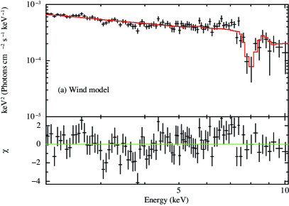
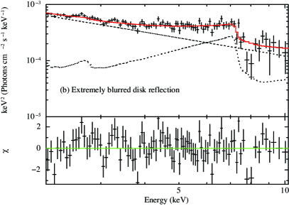
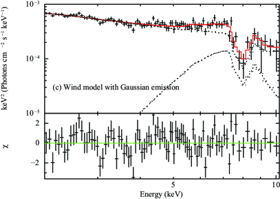
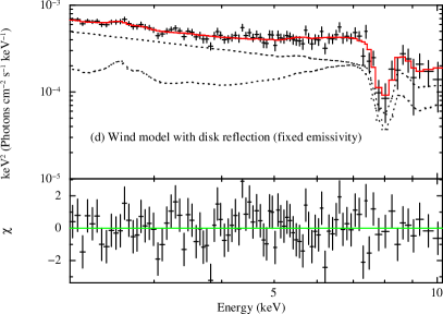
Figure 4: XMM-Newton/pn spectra of Obs12 fitted by (a) wind*powerlaw (top-left), (b) powerlaw+kdblur*reflionx (top-right), (c) wind(powerlaw+zgaus) (bottom-left) and (d) wind(powerlaw+kdblur*reflionx) with emissivity fixed at 3 (bottom-right). The spectra and models are plotted in black and red, respectively. The lower panels show the residuals in units of $\chi$.

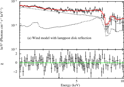
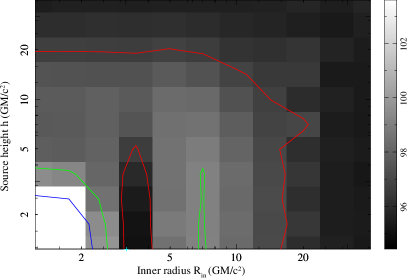
Figure 5: XMM-Newton/pn spectra of Obs12 fitted by the wind model with lamppost disk reflection (wind(powerlaw+relconv_lp*reflionx), left panel) and contour plot of the inner disk radius and the height of the X-ray compact source in the lamppost geometry (right panel). The red, green and blue lines in the contour plot correspond to confidence levels of 68, 90 and 99 percent, respectively. The color map shows the value of $\chi^{2}$ for each parameter grid. The cyan cross is plotted at the best fit, where $h\sim 1$ $r_{\rm g}$ and $R_{\rm in}\sim 3$ $r_{\rm g}$. The model spectrum shown in the left panel corresponds to this extreme solution.

4.2 Application to XMM-Newton and Suzaku data

We re-run monaco with the parameters around the values obtained in the previous section but now put in explicitly the mass of $5\times 10^{6}$ M_⊙, an observed X-ray spectrum with $\Gamma=2.6$ and $L_{\rm x}=2\times 10^{42}$ erg s^-1, and reduce the wind velocity to $0.2c$ but keep the same velocity law.

The result from the previous section suggests that there is rather more line emission compared to absorption than is predicted for the PDS 456 wind geometry. However, a larger solid angle of the wind would necessitate more resolution in $\theta$ and a change in the way of calculating the ionization state. Hence we keep the same wind geometry for the present, and run simulations for $\dot{M}_{\rm wind}/\dot{M}_{\rm Edd}=0.13$, $0.20$, $0.26$. Refitting these to Obs12 gives $\chi^{2}=139.7,132$ and $133$ for $89$ degrees of freedom, respectively. Hence we pick $\dot{M}_{\rm wind}/\dot{M}_{\rm Edd}=0.2$, and apply this model to all the observations of 1H0707. Similarly to PDS 456, we assume that the intrinsic power law stayed constant in spectral index, and that the major change in spectral hardness is produced by a changing absorption from lower ionization species. To describe this absorption, we used a very simple model of partially ionized absorption which can partially cover the source (zxipcf in xspec). This gives an adequate fit to all the PDS 456 spectra, including the hardest (black line in Fig. 2) which bears some similarities to the hardest spectra in 1H0707, which are generally interpreted as reflection dominated (Fabian et al., 2012).

All the spectra (black) and models (red) are plotted in Fig. 6. We also show the background (blue) for each spectrum, so that the signal-to-noise at high energies can be directly assessed. The parameters for each fit are listed in Tab. 3. For Obs8 and Obs12, the absorption component is not included because the significance of adding zxipcf does not exceed the $99$% confidence level of an F-test.

As shown in Fig. 6, our monaco models roughly reproduce the sharp drop around 7.1–7.5 keV in all the observed spectra. The best fit values of inclination angle ranges from $\sim 58^{\circ}$ to $75^{\circ}$. These are all higher than the inclinations inferred for PDS 456, and there is a broader spread in derived inclination angle.

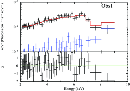
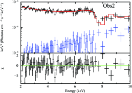
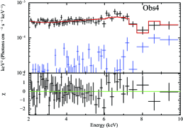
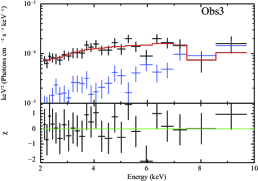
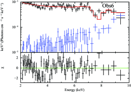
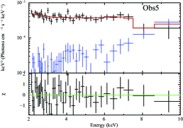
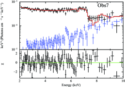
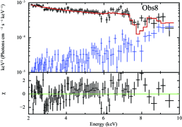
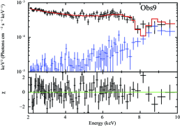
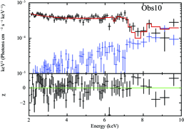
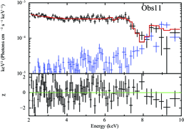
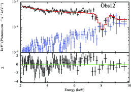
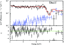
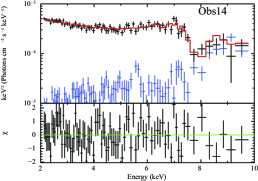
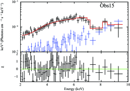
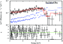
Figure 6: Observed spectra and monaco models with $v=0.2c$ and $\dot{M}_{\rm wind}/\dot{M}_{\rm Edd}=0.2$ for all the observations. The spectra and models are plotted in black and red, respectively. The background spectra are also overplotted in blue. The lower panels show the residuals in units of $\chi$.

Table 3: monaco fit with $v=0.2c$ and $\dot{M}_{\rm wind}/\dot{M}_{\rm Edd}=0.2$ to all the observations of 1H0707.

Name	Continuum absorption			monaco wind	Fit statistics
	$N_{\rm H}$ ($10^{22}$ cm-2)	$\log\xi$	$f_{\rm cov}$	$\theta_{\rm incl}$	$\chi^{2}$/dof	Null probability
Obs1	$28_{-9}^{+83}$	$1.90_{-0.63}^{+0.91}$	$0.85_{-0.03}^{+0.12}$	$74.6_{-5.4}^{+2.8}$	$34.5$/$40$	$0.73$
Obs2	$66_{-43}^{+72}$	$1.90_{-0.87}^{+0.28}$	$0.45_{-0.09}^{+0.45}$	$64.1_{-1.9}^{+2.0}$	$85.2$/$79$	$0.30$
Obs3	$15_{-6}^{+37}$	$<1.63$	$0.68_{-0.05}^{+0.05}$	$64.1_{-6.3}^{+2.8}$	$52.7$/$55$	$0.56$
Obs4	$8.2_{-6.3}^{+18.2}$	$<2.28$	$0.80_{-0.06}^{+0.19}$	$57.9$	$15.1$/$21$	$0.82$
Obs5	$23_{-16}^{+72}$	$<2.14$	$0.28_{-0.09}^{+0.44}$	$68.0_{-1.6}^{+1.5}$	$102.6$/$69$	$0.005$
Obs6	$8.4_{-4.5}^{+90.6}$	$<2.02$	$0.42_{-0.14}^{+0.29}$	$63.4_{-12.7}^{+5.6}$	$28.2$/$34$	$0.75$
Obs7	$151_{-95}^{+11}$	$2.71_{-0.56}^{+0.10}$	$0.71_{-0.25}^{+0.06}$	$68.3_{-1.7}^{+1.7}$	$115.1$/$87$	$0.02$
Obs8	—	—	—	$64.0_{-2.3}^{+2.5}$	$129.12$/$84$	$0.001$
Obs9	$65_{-31}^{+73}$	$<2.26$	$0.42_{-0.21}^{+0.41}$	$58.3_{-1.9}^{+2.9}$	$88.6$/$79$	$0.22$
Obs10	$124_{-109}^{+33}$	$2.71_{-1.90}^{+0.19}$	$0.58_{-0.14}^{+0.16}$	$68.2_{-2.6}^{+2.2}$	$87.4$/$72$	$0.10$
Obs11	$121_{-73}^{+32}$	$2.76_{-0.46}^{+0.21}$	$0.60_{-0.24}^{+0.20}$	$63.1_{-2.6}^{+3.3}$	$100.3$/$81$	$0.07$
Obs12	—	—	—	$60.6_{-1.8}^{+2.5}$	$132.0$/$89$	$0.002$
Obs13	$117_{-63}^{+28}$	$2.73_{-0.31}^{+0.15}$	$0.63_{-0.20}^{+0.13}$	$63.2_{-2.6}^{+2.4}$	$154.9$/$78$	${5\times 10^{-7}}$
Obs14	$181_{-8}^{+203}$	$2.82_{-0.09}^{+0.10}$	$0.82_{-0.08}^{+0.07}$	$63.1_{-2.6}^{+2.3}$	$75.3$/$77$	$0.53$
Obs15	$23_{-6}^{+47}$	$1.61_{-0.78}^{+1.02}$	$0.93_{-0.02}^{+0.04}$	$70.9_{-3.8}^{+3.7}$	$43.1$/$51$	$0.78$
SuzakuObs	$109_{-69}^{+27}$	$2.72_{-1.47}^{+0.07}$	$0.89_{-0.08}^{+0.08}$	$67.0_{-5.4}^{+5.9}$	$97.9$/$86$	$0.18$

¹ No constraints on this parameter were obtained.

4.3 Application to NuSTAR data

A key breakthrough in AGN spectral studies has come from NuSTAR data which extend the energy range of the observed spectra beyond 10 keV and have much better signal-to-noise above 7 keV than the Suzaku or XMM-Newton data (see Fig. 6). 1H0707 has also been observed by NuSTAR, and the resulting spectra can be fit by the extreme relativistic reflection models (Kara et al., 2015).

We extract the NuSTAR data, and follow Kara et al. (2015) in selecting the second NuSTAR dataset, which is a good match to XMM-Newton Obs15. Fig. 7 shows the model fit to Obs15 extrapolated to 30 keV. We note that around half the drop at $\sim 7$ keV is from the wind model alone, while the other half is from the complex lower ionization absorption. There are no additional free parameters, but the model gives a good fit to the higher energy data.

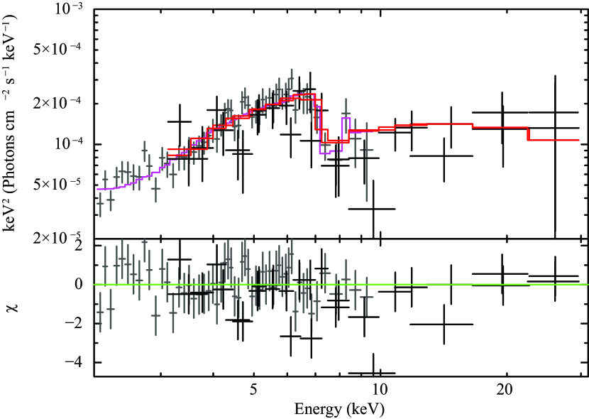
Figure 7: NuSTAR data compared with the best-fit wind model of Obs15. The spectra of XMM-Newton, NuSTAR are plotted in grey and black, while the model lines for XMM-Newton and NuSTAR are plotted in magenta and red, respectively. The lower panels show the residuals in units of $\chi$.

5 Discussion

5.1 Effects of cool clumps

We model the wind using the monaco Monte-Carlo code, which tracks emission, absorption and scattering in a continuous wind geometry (Hagino et al., 2015). In this continuous wind model, all the atoms lighter than iron are almost fully ionized, so that it cannot produce the strong spectral variability seen below the iron line region. Instead, in the archetypal wind source PDS 456, such variability is assumed to be from lower ionization species. In PDS 456 this additional spectral variability can be approximately modeled using partially ionized material which can partially cover the source. We show that this same combination of partial covering by lower ionization material together with the highly ionized wind gives an acceptable fit to the 1H0707 spectra, including the higher energy data from NuSTAR.

The lower ionization material in the wind is likely to be clumped due to the ionization instability for X-ray illuminated material in pressure balance (Krolik et al., 1981). These clumps are cooler and less ionized than the hot phase of the wind, but with lower filling factor. The dramatic dips which are characteristic of the light curves of complex NLS1 like 1H0707 can then be interpreted as occultations by these cool clumps. We note that time dependent, clumpy absorption is typical of both UV line driven disk winds (Proga & Kallman, 2004), and continuum driven winds (Takeuchi et al., 2014).

The partially ionized clumps which partially cover the source imprint some spectral features as well as curving the continuum. Fig. 8 shows the data and model in the entire energy band for the highest (top panel) and lowest (bottom panel) flux states. The data is plotted in black and the total model spectrum is shown by the red line. The model spectrum is separated into absorbed (blue), unabsorbed (green) and a soft X-ray excess component (magenta, see below). The low ionization absorption imprints strong atomic features from oxygen and iron-L below 2 keV in the lowest intensity state, but these are diluted by the X-rays which are not absorbed, so that the total spectrum is almost featureless in the 0.5–2 keV bandpass. Hence it predicts no observable features in the RGS.

The unabsorbed component does not dilute the iron-K features because the absorbed component is dominant at higher energies. The effect of absorption at iron K from the cool clumps alone is shown by the pink line in the inset window of Fig. 8, while the red line in the inset shows the total (cool plus hot phase) absorption. The pink line shows that the cool clumps do imprint iron K$\alpha$ absorption lines around 6.45 keV rest frame from Fe xviii–xx as well as the much stronger K$\beta$ lines around 7 keV rest frame. The K$\beta$ lines blend with the hot phase absorption, while the K$\alpha$ lines have an equivalent width of only a few eV, which is not detectable even with a 300 ks observation with Hitomi for a source as weak as 1H0707. Hence the model is consistent with current and near future limits on spectral features in the data.

A soft excess component (magenta) is added in the model spectrum in Fig. 8 in order to roughly describe the spectrum at low energies. We use a thermal Comptonization model comptt, allowing only the normalization to be free while fixing the shape to parameters typically seen in other AGN, namely a seed photon temperature of 0.05 keV, coronal temperature of $kT=0.2$ keV and optical depth at $\tau=15$ (Done et al., 2012). The plots show that the observed spectrum is roughly reproduced by this model, but there is an excess around 0.8 keV and a deficit between $\sim 1$–2 keV. These differences can be interpreted as broad emission and absorption (P Cygni profile) from oxygen K and iron L-shell transitions, which are naturally expected in the ionized fast wind, but are not included in our current Monte-Carlo code. Hence these features in the data are not well described by the model used here, which is tailored instead to iron K. Nonetheless, we do expect that similar features would be produced by including emission and absorption from cool clumps in our wind model.

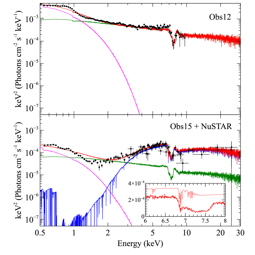
Figure 8: The observed data and model of the highest flux state (Top: Obs12) and the lowest flux state (Bottom: Obs15 and the NuSTAR data) plotted over a wide energy range. The absorbed spectrum is shown as the blue line, the unabsorbed in green, the total in red, and the observed data in black. A soft X-ray excess component with typical parameters is also plotted in magenta to show the spectrum at lower energies below 2 keV. There are no spectral features predicted below 2 keV due to the dilution by the unabsorbed (or reflected/scattered) flux (green). There are absorption lines from Fe xviii–xx produced by cool clumps (pink line in a small window inside bottom panel) but the K$\alpha$ lines at $\sim 6.45$ keV are not detectable even with 250 ks of Hitomi, and the higher energy lines merge with the hot phase of the wind (red line in a small window).

Our model is currently incomplete as these clumps should also reflect/emit as well as absorb, adding to the reflection/emission from the highly ionized phase of the wind which is included in our monaco simulation. This reflection/emission from the composite wind could dominate during the dips, where the cool clumps probably completely cover the source itself. We also envisage the cool clumps to be entrained in the wind, so the atomic features should also be blueshifted/broadened by the wind velocity structure. This means that the cool phase of the wind also contribute to the total wind kinetic luminosity which has so far been neglected.

The clumpy structure can also play an important role for a characteristic time lags observed in 1H0707. The observations show a complex pattern of lags between soft and harder energies, with the soft band leading for slow variability, and lagging for fast variability (Fabian et al., 2009; Zoghbi et al., 2010). In the relativistic reflection picture, this can be explained by a partially ionized disk, where reflection is weaker at 2–4 keV than at lower or higher energies. Thus, reflection dominates in the soft band, while the intrinsic continuum dominates in the intermediate band at a few keV. Reflection follows the continuum, but with a lag from the light travel time from the source to the reflector, giving the soft (conventionally referred to as a ‘negative’) lag at high frequencies. The positive lag at lower frequencies is probably from propagation of fluctuations through the accretion flow. On the other hand, a full spectral-timing model including both the positive and negative lags for PG 1244+026, another AGN with very similar mass and mass accretion rate to 1H0707, gives the observed lag of 200 s seen in PG 1244+026 from reprocessing by material extending from 6–12$R_{\rm g}$ (assuming a mass of $10^{7}$M_⊙: Gardner & Done, 2014). In this interpretation, this lag is due to the illuminating hard X-ray flux which is not reflected but thermalized and re-emitted as quasi-blackbody radiation. Adding multiple occultations by clumps onto the same full spectral-timing model reduces the predicted lags to 50 s, similar to the 30 s observed in 1H0707 but without requiring a small reflector distance (Gardner & Done, 2015). Thus cool clumps may be able to explain both the time averaged spectrum and the extremely short lags without requiring lightbending from a small corona close to the event horizon of an extreme spin black hole, though it remains to be seen whether they can fit the lag-energy spectra as well as the lag frequency spectra (Gardner & Done, 2015). However, we note that the lamppost model itself also has difficulty fitting the details of the lag-energy spectra (Wilkins et al., 2016). Their alternative geometry of an extended corona may give a better fit to the lag-energy spectra, but it seems unlikely to be able to simultaneously explain the deep dips in the light curves which can be explained in the lamppost model by the very small source approaching the horizon.

5.2 Wind geometry

Our specific wind model is probably not unique in terms of wind geometry and velocity structure. In particular, we used the same wind solid angle of $\Omega/4\pi=0.15$ in 1H0707 as for PDS 456. This is likely to be appropriate for PDS 456 if there is indeed some component of UV line driving to the wind. It is because numerical studies show that this driving mechanism results in time variable but fairly narrow wind streamlines. However, continuum radiation driving is much more likely in 1H0707, in which case the numerical simulations predict a wider opening angle wind. Future work should simulate winds with a larger opening angle, which would require correspondingly larger mass loss rates in order to keep the same absorption column density.

The wider opening angle wind should also result in stronger line emission, so that this may give a better fit to some of the remaining residuals. However, we caution that all these spectra are co-added, integrating over dramatic short timescale variability so steady state models may not be appropriate.

6 Conclusions

We can successfully reproduce the range of spectra seen from 1H0707 with absorption in a wind from the inner disk. The strong spectral drop is produced by our line of sight cutting across the acceleration region where the wind is launched. In this region, we see the absorption line over a wide range of velocities, making a very broad feature. Since the column density in the wind is large, the broad absorption line merges into the absorption edge, which further depresses the spectrum at higher energies.

Our wind model probably inappropriate to this source as discussed in section 5. The time variability and the low ionization absorption in the observed spectra seems to be consistent with an existence of cool clumps in the wind. This clumps are naturally expected due to the instability of the wind. Also, a larger opening angle of the wind would probably give better fits to the observed data. This implies the continuum radiation driving mechanism, which is expected in the super Eddington accretion.

Nonetheless, the wind model presented here can fit the overall 2–30 keV spectra from 1H0707. Unlike the lamppost models, it does not require that the black hole has extreme spin, nor does it require that we have a clean view of a flat disk, nor does it require that iron is 7–20 times overabundant. We suggest that the extreme iron features in 1H0707 arise more from absorption/scattering/emission from an inner disk wind than from extreme gravity alone.

References

- Allison et al. (2006) Allison J., et al., 2006, IEEE Trans. Nucl. Sci., 53, 270
- Boller et al. (2002) Boller T., et al., 2002, MNRAS, 329, L1
- Boroson (2002) Boroson T. A., 2002, ApJ, 565, 78
- Chartas et al. (2002) Chartas G., Brandt W. N., Gallagher S. C., Garmire G. P., 2002, ApJ, 579, 169
- Dauser et al. (2013) Dauser T., Garcia J., Wilms J., Bock M., Brenneman L. W., Falanga M., Fukumura K., Reynolds C. S., 2013, MNRAS, 430, 1694
- Done & Jin (2016) Done C., Jin C., 2016, MNRAS, 7
- Done et al. (2007) Done C., Sobolewska M. A., Gierliński M., Schurch N. J., 2007, MNRAS, 374, L15
- Done et al. (2012) Done C., Davis S. W., Jin C., Blaes O., Ward M., 2012, MNRAS, 420, 1848
- Fabian et al. (2004) Fabian A. C., Miniutti G., Gallo L., Boller T., Tanaka Y., Vaughan S., Ross R. R., 2004, MNRAS, 353, 1071
- Fabian et al. (2009) Fabian A. C., et al., 2009, Nature, 459, 540
- Fabian et al. (2012) Fabian A. C., et al., 2012, MNRAS, 419, 116
- Gallo et al. (2004) Gallo L. C., Tanaka Y., Boller T., Fabian A. C., Vaughan S., Brandt W. N., 2004, MNRAS, 353, 1064
- Gardner & Done (2014) Gardner E., Done C., 2014, MNRAS, 18, 1
- Gardner & Done (2015) Gardner E., Done C., 2015, MNRAS, 448, 2245
- Hagino et al. (2015) Hagino K., Odaka H., Done C., Gandhi P., Watanabe S., Sako M., Takahashi T., 2015, MNRAS, 446, 663
- Hashizume et al. (2015) Hashizume K., Ohsuga K., Kawashima T., Tanaka M., 2015, PASJ, 67, 58
- Higginbottom et al. (2014) Higginbottom N., Proga D., Knigge C., Long K. S., Matthews J. H., Sim S. A., 2014, ApJ, 789, 19
- Inoue & Matsumoto (2001) Inoue H., Matsumoto C., 2001, Advances in Space Research, 28, 445
- Jiang et al. (2014) Jiang Y.-F., Stone J. M., Davis S. W., 2014, ApJ, 796, 106
- Kara et al. (2015) Kara E., et al., 2015, MNRAS, 449, 234
- Krolik et al. (1981) Krolik J. H., McKee C. F., Tarter C. B., 1981, ApJ, 249, 422
- Miller et al. (2007) Miller L., Turner T. J., Reeves J. N., George I. M., Kraemer S. B., Wingert B., 2007, A&A, 463, 131
- Miller et al. (2008) Miller L., Turner T. J., Reeves J. N., 2008, A&A, 483, 437
- Miller et al. (2010) Miller L., Turner T. J., Reeves J. N., Braito V., 2010, MNRAS, 408, 1928
- Miniutti & Fabian (2004) Miniutti G., Fabian A. C., 2004, MNRAS, 349, 1435
- Mizumoto et al. (2014) Mizumoto M., Ebisawa K., Sameshima H., 2014, PASJ, 66, 122
- Nardini et al. (2015) Nardini E., et al., 2015, Science, 347, 860
- Odaka et al. (2011) Odaka H., Aharonian F., Watanabe S., Tanaka Y., Khangulyan D., Takahashi T., 2011, ApJ, 740, 103
- Ohsuga & Mineshige (2011) Ohsuga K., Mineshige S., 2011, ApJ, 736, 2
- Ponti et al. (2010) Ponti G., et al., 2010, MNRAS, 406, 2591
- Proga (2003) Proga D., 2003, ApJ, 585, 406
- Proga & Kallman (2004) Proga D., Kallman T. R., 2004, ApJ, 616, 688
- Proga et al. (2000) Proga D., Stone J. M., Kallman T. R., 2000, ApJ, 543, 686
- Reeves et al. (2003) Reeves J. N., O’Brien P. T., Ward M. J., 2003, ApJ, 593, L65
- Reeves et al. (2009) Reeves J. N., et al., 2009, ApJ, 701, 493
- Ross & Fabian (2005) Ross R. R., Fabian A. C., 2005, MNRAS, 358, 211
- Sa̧dowski & Narayan (2016) Sa̧dowski A., Narayan R., 2016, MNRAS, 456, 3929
- Sim et al. (2008) Sim S. A., Long K. S., Miller L., Turner T. J., 2008, MNRAS, 388, 611
- Sim et al. (2010) Sim S. A., Miller L., Long K. S., Turner T. J., Reeves J. N., 2010, MNRAS, 404, 1369
- Takeuchi et al. (2014) Takeuchi S., Ohsuga K., Mineshige S., 2014, PASJ, 66, 48
- Tatum et al. (2012) Tatum M. M., Turner T. J., Sim S. A., Miller L., Reeves J. N., Patrick A. R., Long K. S., 2012, ApJ, 752, 94
- Tombesi et al. (2010) Tombesi F., Cappi M., Reeves J. N., Palumbo G. G. C., Yaqoob T., Braito V., Dadina M., 2010, A&A, 521, A57
- Tombesi et al. (2012) Tombesi F., Cappi M., Reeves J. N., Braito V., 2012, MNRAS, 422, L1
- Turner et al. (2007) Turner T. J., Miller L., Reeves J. N., Kraemer S. B., 2007, A&A, 475, 121
- Watanabe et al. (2006) Watanabe S., et al., 2006, ApJ, 651, 421
- Wilkins et al. (2016) Wilkins D. R., Cackett E. M., Fabian A. C., Reynolds C. S., 2016, MNRAS, 458, 200
- Zoghbi et al. (2010) Zoghbi A., Fabian A. C., Uttley P., Miniutti G., Gallo L. C., Reynolds C. S., Miller J. M., Ponti G., 2010, MNRAS, 401, 2419