Visual Generalized Coordinates ^∗

Abstract

An open problem in robotics is that of using vision to identify a robot’s own body and the world around it. Many models attempt to recover the traditional C-space parameters. Instead, we propose an alternative C-space by deriving generalized coordinates from $n$ images of the robot. We show that the space of such images is bijective to the motion space, so these images lie on a manifold $\mathcal{V}$ homeomorphic to the canonical C-space. We now approximate this manifold as a set of $n$ neighbourhood tangent spaces that result in a graph, which we call the Visual Roadmap (VRM). Given a new robot image, we perform inverse kinematics visually by interpolating between nearby images in the image space. Obstacles are projected onto the VRM in $O(n)$ time by superimposition of images, leading to the identification of collision poses. The edges joining the free nodes can now be checked with a visual local planner, and free-space motions computed in $O(nlogn)$ time. This enables us to plan paths in the image space for a robot manipulator with unknown link geometries, DOF, kinematics, obstacles, and camera pose. We sketch the proofs for the main theoretical ideas, identify the assumptions, and demonstrate the approach for both articulated and mobile robots. We also investigate the feasibility of the process by investigating various metrics and image sampling densities, and demonstrate it on simulated and real robots.

I Introduction

(a)

(b)

(c)

(d)

(e)

(f)

Figure 1: Overview example: (a) A 2-link planar arm from [1] - both joints rotate fully around (C-space is a torus). (b) the canonical C-space from [1] and a path for the poses in (a). (c) Fifty of 20000 sample images from a simulation of a similar arm. (d) The image manifold $\mathcal{V}$, visualized here in $\mathbb{R}^{3}$ using the Isomap algorithm [2], shows that the robot images - from a $570\times 570$-dimensional image space - lie on the 2-D surface of a torus. Thus the Visual Configuration Space (VCS) has the same structure as the canonical C-Space. The Visual Roadmap (VRM) is a graph embedded on the VCS, represented as a set of tangent spaces (charts). Red points are non-free configurations, identified by overlapping background-subtracted robot images with obstacle images. (e) Workspace trajectory between the two poses of (a), found using the VRM. (f) Path (blue dots) shown on the cut-open torus. Note that the VCS dimension $q_{2}$ (vertical axis) has flipped $\theta_{2}$ in (b), and both axes are circularly shifted.

Humans and animals routinely use prior sensorimotor experience to build motor models, and use vision for gross motor tasks in novel environments. Achieving similar abilities, without having to calibrate a robot’s own body structure, or estimate exact 3-D positions, is a touchstone problem for robotics (e.g. see [3] ch.9). Such an approach would enable a robot to work in less controlled environments, as is being increasingly demanded in social and interactive applications for robots.

There have been two methods for approaching this problem - either based on learning a body schema [4, 5, 6, 7, 8, 9], or by fitting a canonical robot model [10]. Body schema approaches have not scaled up to full scale robotic models or used for global motion planning, and robot model regression requires intrusive structures on the robot  [11] and even then it cannot sense the environment.

Another approach, visual servoing attempts to estimate the motion needed for small changes in image features. However, visual servoing models cannot construct models spanning large changes in robot pose, since the pseudo-inverse of the image Jacobian can be computed only over small motions. Recently, global motion planning algorithms have been proposed by stitching together local visual servos [12], but these require that the goal be constantly visible.

I-A Visual Generalized Coordinates

The notion of Configuration Space is fundamental to conceptualizing multi-body motion. The configuration of a system with $d$ degrees of freedom can usually be specified in terms of $d$ independent parameters, known as generalized coordinates (GC). Thus, for a planar robot arm with two links, as in fig. 1a, the canonical choice for GC is to use the joint angles $(\theta_{1},\theta_{2})$. However, this is only one of many (potentially infinite) choices of coordinates, each resulting in a different C-space. GCs need not specify joint angles or any motion parameter - they just need to uniquely specify the pose. One of our main aims is to show that an alternate GC can be learned from the robot’s appearance alone, i.e. from a set of images. These visual coordinates are homeomorphic to the canonical coordinates - as in fig. 1d, where we note that the image manifold (the Visual Configuration Space, VCS) is a torus, just like the canonical $(\theta_{1},\theta_{2})$ manifold. This is particularly notable since the image dimensionality $\approx 3\times 10^{5}$, so the image space is enormous; yet the images that can show robot poses lie on this tiny two-dimensional subspace. This can be explained by noting that the probability of a random image being a robot image is vanishingly small. The Visual Manifold theorem below formalizes these claims.

Such a system would have many advantages. For example, if an unknown robot is given to us, we can learn its VCS by observing a random set of poses as it moves. In fact, this idea draws inspiration from proposals for how an infant learns to use its limbs [13, 14]. Now if a task is specified visually - such as an object to grasp - the pose desired for executing it may be easier to specify in terms of its image, or that of its gripper (the set of gripper images also form an equivalent manifold). Given a novel goal image, the system can interpolate between nearby known poses to reach the desired pose (inverse kinematics). Assuming we have a controller that can repeat previously seen poses, the robot can now reach for the object by traversing a set of landmark images. Obstacles introduced now can be superimposed on the set of images to identify collision configurations. Given a set of possibly multiple cameras, this enables the system to find paths avoiding obstacles. Parts of its body or workspace that is accessed repeatedly can have a finer model (by sampling more images from this part of the workspace). The system can cluster task trajectories to learn action schemas etc. One could then “imagine” the consequence of a motor command, and compare these quickly to find discrepancies [15]. All this is done without any knowledge of robot kinematics or shape, its environment, or even the camera poses.

The model proposed here has some constraints. It requires that the set of cameras be able to see the robot in all its poses. Thus, it is more suited for articulated robot arms, though it would also work for a mobile robot seen from a roof camera. Also, it requires that every pose of the robot must be visually distinguishable - i.e. different poses should look different from at least one of the camera views.

Our main contributions are a) to show that configuration spaces based on robot images, and not joint angles, exist; b) present a sampling-based algorithm that takes a large set of robot pose images, and constructs piecewise approximations in terms of local neighbourhoods on the image manifold. c) demonstrate how such a visual C-space can be equivalently used to find a roadmap and identify poses (inverse kinematics), and plan motions.

Section II gives an overview of the algorithm. Section III presents a theoretical analysis proving the existence of the VCS (Visual Manifold Theorem) and that obstacles in the workspace can be modelled via image superposition (Visual Collision Theorem). Section IV constructs a discrete model of the image manifold $\mathcal{V}$ by stitching together neighbouring images into a graph that we call the Visual Roadmap (VRM). This is analogous to roadmaps used in sampling based motion planning [1, 16]. During the VRM construction, only immovable parts of the environment are present; obstacles etc can be introduced later. For motion planning purposes, the robot foreground in each image is obtained by removing the fixed background; these are superimposed on an obstacle image to identify the collision states. Note that this is equivalent to modelling the obstacle as the convex hull of the visibility cones (Fig. 5). Each edge between neighbouring free space nodes is now tested using one of several visual local planners (section IV-B). Now, given images for the Start and Goal poses of the robot, one can add edges from these to the nearest safe neighbours in the VRM, and find a path on the graph. Section V presents an empirical analysis of the various choices for image space metrics and local planners, and section VI shows some demos on real robots.

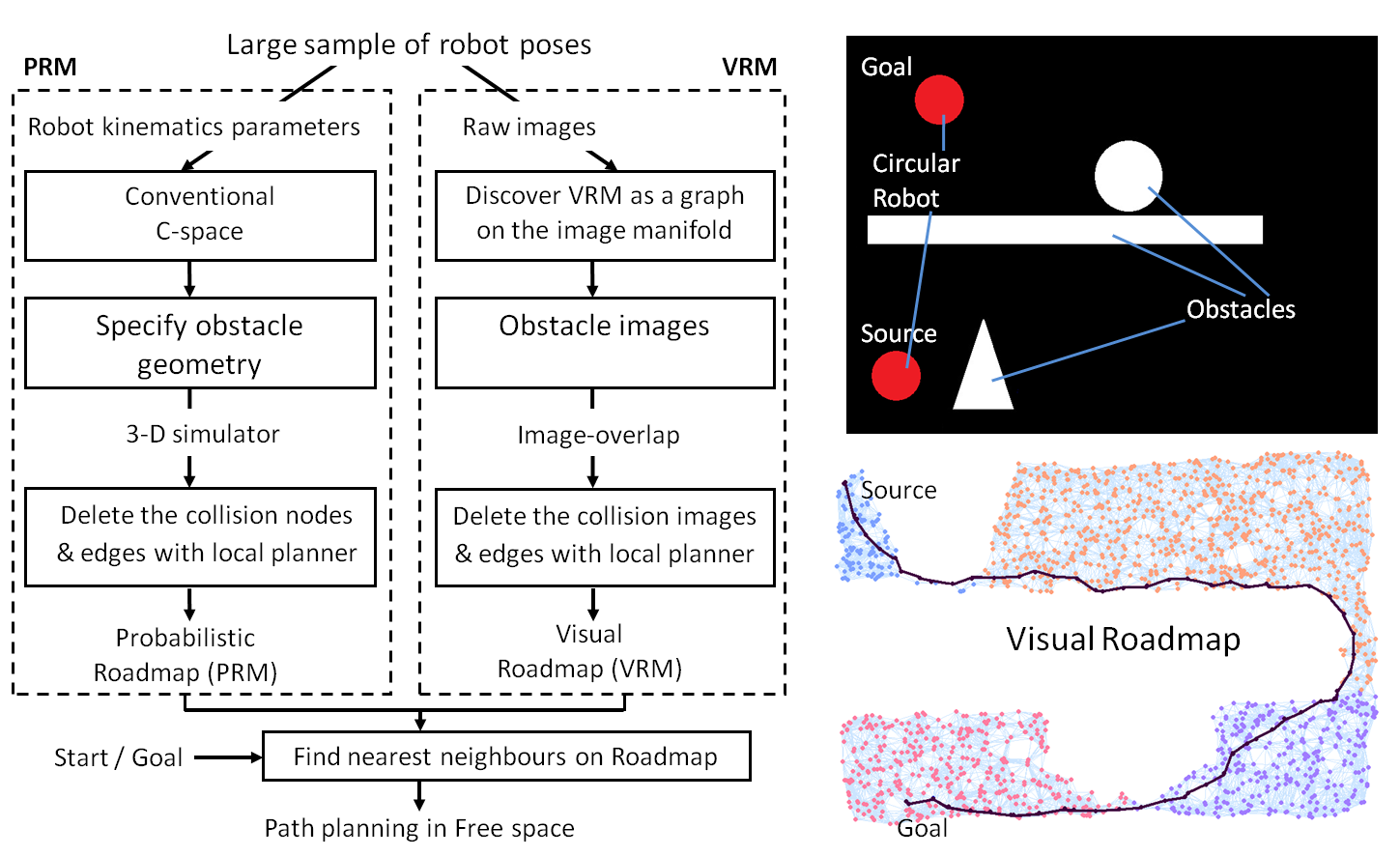
Figure 2: Visual Roadmap as an analogue of Probabilistic Roadmap (PRM). In the Visual Roadmap (VRM) approach, a graph is constructed from the neighbourhoods in image space. This requires no knowledge of robot kinematics or geometry. Just as with PRM, one now deletes nodes overlapping the obstacles, and constructs a path on the remaining edges of the graph. The process is illustrated with a simulated mobile robot : the manifold (bottom right) is constructed solely from a sample of 2000 images. The VRM graph is shown with all obstacle nodes removed and a path identified for a given source and goal. As in fig. 1f, manifold discovery preserves topology but may flip / deform the map.

II Algorithm overview and inverse kinematics

Going from a configuration $q\in\mathcal{Q}$ to the workspace robot shape and its inverse - known as forward and inverse kinematics - traditionally involves careful assignment of coordinate frames and complex transformations between these. In the Visual Generalized Coordinates approach, once we have the VRM, inverse kinematics can be computed for any desired pose, presented as an image $x$. To do this, we find the images nearest to $x$, and interpolate between these on the local chart on $\mathcal{V}$. Now, to plan motions, traditional methods require explicit knowledge of obstacle geometry as well as a simulator for testing collisions. Both these are replaced by visual intersection

Fig. 2 shows an overview of the VRM algorithm, demonstrated on a simulated mobile robot. The idea of the Visual Roadmap is an analog to the Probabilistic Roadmap, in that it is a graph $\{V,E\}$ where $V$ is the set of images sampling the entire workspace, and $E$ the edges connecting local neighbours. This is the heart of this work, where the conventional configuration description $\mathcal{Q}$ (e.g. the joint angle space) is replaced by a completely different GC based on images. The latent space ${\cal V}$ here is discovered from images, and is homeomorphic to $\mathcal{Q}$.

II-A Visual Roadmap

Discovering Visual Generalized Coordinates requires us to find the neighbours of an image in image space. This requires an image metric - e.g. Fig. 2 uses a simple euclidean metric. An alternate metric may be to evaluate the swept volume between two poses. This can often be effectively approximated by the maximum distance covered by any point [17]. (see section IV-B2. Poorer metrics may corrupt the neighbourhood and call for much denser samples. Thus, we find that track distance based metrics, or Hausdorff measures, outperform the Euclidean metrics and require order of magnitude less samples for the same results V-B.

Image space neighbourhoods are then used to construct a local-PCA based nonlinear manifold [18]. The graph based on the neighbourhoods is the VRM. We observe that there can be situations where multiple robot poses look alike to the imaging system (see fig. 4). A critical assumption underlying our approach is that each pose is distinguishable at least from one camera. This is the Visual distinguishability assumption. In practice, most robots already meet this criteria.

We thus show that the system can discover a compact non-metric model, that retains the structure of the conventional Configuration Space $\mathcal{Q}$, but one that is derived solely based on a dense latent space discovery. The discovered lower-dimensional space $\mathcal{V}$ can be mapped to the robot image space $\mathcal{I}$ and to the traditional C-space $\mathcal{Q}$. We also observe that these mappings are the visual analogues for forward and inverse kinematics as in traditional robotics.

III Visual Configuration Space

In order to understand the idea of the Visual Configuration Space, let us consider the space of images of a robot $\mathcal{I}$ (e.g. for the 2-DOF robot of fig. 1). The input Images are high dimensional - if each image is $640\times 480$ (approximately $10^{5}$) pixels, then $\mathcal{I}\subset\mathbb{R}^{3\times 10^{5}}$. However, given an image $x$ in $\mathcal{I}$, it can be altered as many ways as the degrees of freedom $d$, without the resulting image leaving $\mathcal{I}$. So the intrinsic dimensionality of $\mathcal{I}$ is 2. Further, as the links keep rotating, in the end the image sequence returns to the original image. Thus the topology of $\mathcal{I}$ is not euclidean ($\mathbb{R}^{2}$), but a $d$-torus ($S^{1}\times S^{1}$ for the 2-DOF robot). Also, the image space changes smoothly as it moves, and so the mapping is diffeomorphic. Thus if $\mathcal{V}$ is a smooth dense latent space for $\mathcal{I}$, then every image neighbourhood in $\mathcal{I}$ maps to a neighbourhood in $\mathcal{V}$, and these maps change smoothly as one moves through the poses of the robot.

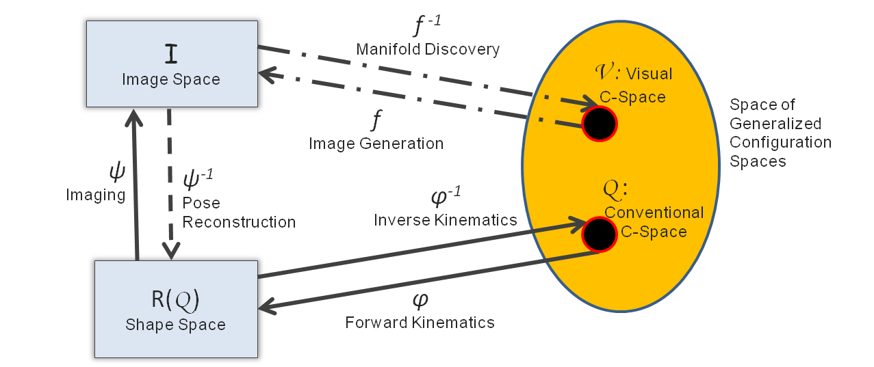
Figure 3: Robot pose, Robot shape, Image and Visual spaces: In order for visual generalized coordinates to exist, two robot poses cannot generate the same image. If this condition holds, we show that any coordinate for the image manifold constitutes a generalized coordinate system. Under such conditions, the map $\psi\circ\phi$ between $\mathcal{Q}$, the shape space $R(\mathcal{Q})$ and the image space $\mathcal{I}$ is bijective, and the image manifold does not self-intersect. The latent space $\mathcal{V}$ is a specification of generalized coordinates on the image manifold, and is a member of the collection of C-spaces. The bijective map $f:\mathcal{V}\leftrightarrow\mathcal{I}$ relates robot images to unique points in $\mathcal{V}$. Given sample images $X\subset\mathcal{I}$, we estimate $\mathcal{V}$ via a Local Tangent Space approximation of the manifold, and do not explicitly compute the mappings $f$ and $f^{-1}$ (coordinates in $\mathcal{V}$ - shown as dashed lines).

While these properties hold for the continuous image space, in practice we work with a representative sample $X=\{x_{1}...x_{n}\}\subset{\cal I}$. There are a number of manifold discovery algorithms that one could use (e.g. Isomap [2]). However, such methods have difficulty in introducing new data points and in interpolating local data, so we avoid computing the manifold altogether, and restrict ourselves to a piecewise algorithm, as in [18, 19].

We now establish the conditions under which the space of all images of the robot would also form a homologous manifold.

III-A Visual Distinguishability

In general, the imaging transformation $\phi$ is not invertible - i.e. the 3D positions are not recoverable from the image. It is only because the image is being generated under motion constraints, that one can find a map from the image space to a unique low-dimensional map. However, this does not hold in all situations (fig. 4); hence we require that in practice, there be some colour textures on the robot body, or a restricted range of motion, that permits distinguishability of all robot poses. This is the visual distinguishability assumption.

Let $R_{q}$ be the set of all points of the workspace occupied by the robot (its volume) in configuration $q$, and let $R(\mathcal{Q})=\{R_{q}:q\in\mathcal{Q}\}$ be the set of all robot shapes. Let $\phi:\mathcal{Q}\rightarrow R(\mathcal{Q})$ and $\psi:R(\mathcal{Q})\rightarrow\mathcal{I}$ be the functions that map a configuration to a shape and a shape to an image respectively. Then the visual distinguishability assumption requires that the function $\psi\circ\phi:\mathcal{Q}\rightarrow\mathcal{I}$ be a bijection as illustrated in fig. 3.

The imaging transformation $\psi\circ\phi$ maps each configuration $q$ to an image $I_{q}$ projected by the boundary $\delta R_{q}$ of shape $R_{q}$. If the visual distinguishability assumption holds, then both $\phi$ and $\phi^{-1}$ exist and are continuous, because small changes in the robot configuration lead to small changes in its shape and the corresponding images and vice versa. So, whenever $\mathcal{Q}$ is a manifold, $\mathcal{I}$ is also a manifold of the same dimension (i.e., for a $d$ DOF robot the image space is a $d$-dimensional manifold). This is the manifold on which the Visual Roadmap (VRM) is constructed.

III-B Visual Manifold Theorem

Definition 1.

A Smoothly Moving Piece-wise Rigid body (SMPR) is any system with a smooth map from its configuration space to its shape space.

Lemma 1.

For a $d$-DOF SMPR, the configuration space is a $d$-dimensional topological manifold.

Definition 2.

A visually distinguishable system is one for which the visual distinguishability assumption holds.

Hence, for a visually distinguishable SMPR, $\psi\circ\phi:\mathcal{Q}\rightarrow\mathcal{I}$ is a homeomorphism.

Theorem 1.

Whenever $\mathcal{Q}$ is a manifold, $\mathcal{I}$ is a manifold of the same dimension.

Proof.

The imaging transformation $\psi\circ\phi$ maps each configuration $q$ to an image $I_{q}$ projected by the boundary $\delta R_{q}$ of shape $R_{q}$. If the visual distinguishability assumption holds, then both $\phi^{-1}$ and $\psi^{-1}$ exist, and the image space $\mathcal{I}$ is homeomorphic to the configuration space $\mathcal{Q}$. Hence $\mathcal{I}$ constitutes a manifold of the same dimension as that of $\mathcal{Q}$, whenever $\mathcal{Q}$ is a manifold. ∎

Fig. 9 row 1(c) shows a plot of the residual variance against degrees of freedom for a 2-DOF SCARA arm; the model is clearly captured by a manifold of intrinsic dimensionality two.

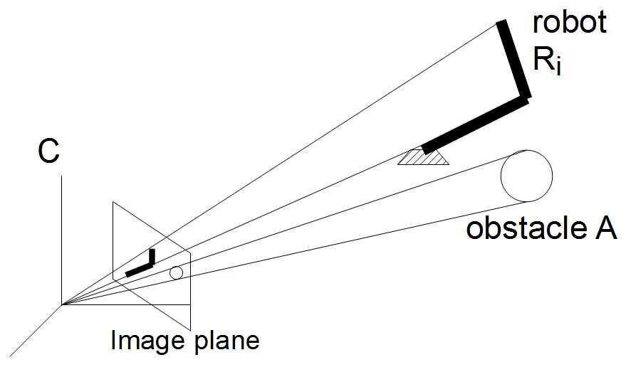
Figure 4: Imaging the workspace. The robot and obstacle lie along the projection bundle from the optical center via their image regions in the virtual image plane (left). If these bundles do not intersect, $R\cap A=\emptyset$. However, the converse is not true. Mid & right: Images of CRS A465 6-axis robot appear to be neighbouring poses, but close observation reveals that the base joint $\theta_{1}$ has rotated by nearly 180 degrees, while $\theta_{2}$ and $\theta_{3}$ have changed sign. Such situations are avoided in the analysis by additional cameras (e.g. on the gripper), or by adding decals. Another method for handling such cases would be to jointly map motor and visual data onto the same fused manifold

III-C Difficulties with Manifold discovery algorithms

For robots which involve a motion with an $S^{1}$ topology, the C-space and hence the VRM space is not globally Euclidean. For example, the C-space of a freely-rotating 2-DOF articulated robot is $S^{1}\times S^{1}=\bf{T}^{2}$, which is a torus [20]. Traditional nonlinear dimensionality reduction (NLDR) algorithms (e.g. [2]) assume that the target space for dimensionality reduction is a euclidean space (a subspace of $\mathbb{R}^{n}$). This means that a $d$-torus manifold, which is $d$-dimensional, cannot be globally mapped to an $\mathbb{R}^{d}$ space, with which it is locally homeomorphic. Another practical difficulty with NLDR algorithms is that it is very challenging to add new points to the manifold without recomputing the entire structure.

At the same time, the global non-linear coordinate is little more than a convenience, and does not materially affect the modelling, which can be done in a piecewise linear manner. Thus, we avoid computing global coordinates altogether, and use the local neighbourhood graphs for planning global paths and local tangent spaces, discovered using Principal Component Analysis (PCA), for checking the safety of edges (local planner). These local tangent spaces, in theory, correspond to charts which when stitched together form an atlas for the image manifold.

We next describe how obstacles are mapped on the VCS for collision detection.

Figure 5: Conservative modelling of 3-D obstacles. For 3-D obstacles, the robot image must not overlap with the obstacle in at least one camera view. If some part of the robot occludes the obstacle in the cones for all the cameras the system will consider it to be a collision situation.

III-D Collision Detection in VCS

In the imaging process, robot and obstacle are mapped to a bundle of rays converging on the camera optical center (figure 4).

Let ${}^{C}R_{i}$ be the bundle subtended at camera optical center ${}^{C}O$ by the robot in configuration $q^{(i)}$, ${}^{C}A$ be the bundle subtended at ${}^{C}O$ by the obstacle $A$ and ${}^{I}R_{i}$, ${}^{I}A$ be the image regions corresponding to the robot and the obstacle.

Lemma 2.

If ${}^{C}R_{i}\cap^{C}A=\emptyset$ then $A\cap R(q^{(i)})=\emptyset$.

Thus, robot configurations for which the bundles do not intersect with the obstacle bundle are guaranteed to be in the free space ${\mathcal{F}}$. Note that the converse is not true.

Lemma 3.

${}^{C}A\cap^{C}R=\emptyset$ iff ${}^{I}A\cap^{I}R=\emptyset$.

Theorem 2.

(Visual Collision Theorem) For a robot in a given pose $q^{(i)}$, if ${{}^{I}}R_{i}\cap{{}^{I}}A=\emptyset$, then $q^{(i)}\in{\mathcal{F}}$.

We note that the above is a necessary condition, but it is often rather conservative. Indeed, the inverse condition defines occlusion situations: where $A\cap R=\emptyset$ but ${}^{C}R\cap^{C}A$ is non-null. This limitation is a result of the information loss in the imaging process. These can be cause particular difficulties for articulated arms. In such cases, one may use multiple cameras; since the Visual Collision Theorem holds for all cameras, we may define any space as free if ${}^{C}R\cap^{C}A=\emptyset$ in at least one view. In this situation, both robot and obstacle are less conservatively modelled as the intersection of multiple cones.

In general, for non-orthographic projections, the higher the ratio of camera distance/focal length, the tighter the bound. (e.g the Scara robot arm in section VI-A).

IV Visual Roadmap and Motion Planning Algorithms

A colour image sample $X\in\mathbb{R}^{p\times n}$ where each $r\times c\times 3$ RGB image is represented as a $p$-dimensional vector $(p=3rc)$ of intensities. We assume that the images are captured against a fixed background, which can be eliminated, so that in the foreground images, a pixel is non-zero if and only if it belongs to the robot. Image $x_{i}\in X$ corresponds to configuration $q_{i}\in Q$. Let $d(x_{i},x_{j})$ be a suitable metric (e.g. Euclidean distance between the image vectors), and let $\mathcal{N}(x)$ be the set of $k$-nearest neighbours of $x$.

Next, we construct a graph $G(V,E)$ over the $n$ nodes so that $v_{i}\in V$ corresponds to image $x_{i}$ (or configuration $q_{i}$). We add an edge between two nodes $v_{i}$ and $v_{j}$ if either $x_{i}\in\mathcal{N}(x_{j})$ or $x_{j}\in\mathcal{N}(x_{i})$ and assign edge weight $d(x_{i},x_{j})$. We call this graph the Visual Roadmap (VRM).

IV-A VRM with Static Obstacles

For handling obstacles, we take the background subtracted images, and test this intersection with the obstacle image. Non-empty overlaps imply that the configuration is not free and we remove the corresponding node and its incident edges from $G$. If $b\in\mathbb{R}^{p}$ is the obstacle image vector, then the set of nodes to be removed from $G$ is $V_{collision}=\{v_{i}:x_{i}*b\neq\bf{0}\}$, where $*$ denotes entry-wise product (Hadamard product) and $\bf{0}$ is the zero-vector. Thus, we obtain a modified graph $G^{\prime}(V^{\prime},E^{\prime})$ in which every node represents a free configuration. However, the edges may still touch some part of the obstacle in an intermediate pose. Guaranteeing edge-safety is the problem of local planner below. Note that this process applies to any number of static obstacles.

IV-B Local Planner in VRM

We say that an edge $(u,v)$ of $G$ is safe, if the geodesic from $u$ to $v$ on the configuration manifold does not contain any image that overalps with an obstacle. The geodesic is approximated by the shortest path on $G$. Given that the nodes $V$ are in the free space, we need to guarantee that every edge is also safe. We describe three local planners that work with robot images and can be used on visual roadmaps. To make sure that an edge is safe, these methods construct a new image that in estimates the swept volume of the robot in the workspace and check this image for collision. Figure 6 shows examples of images generated by these local planners.

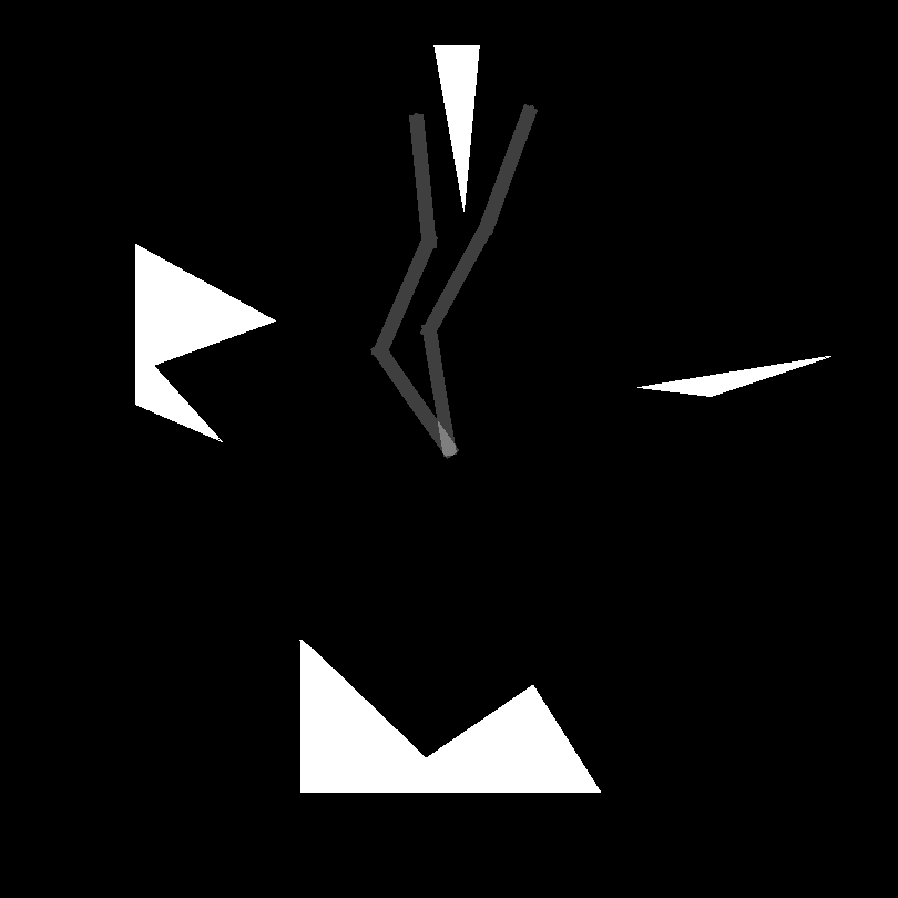
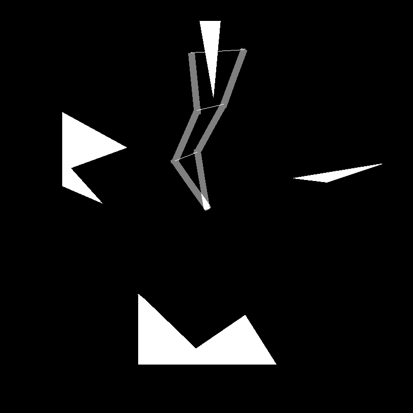
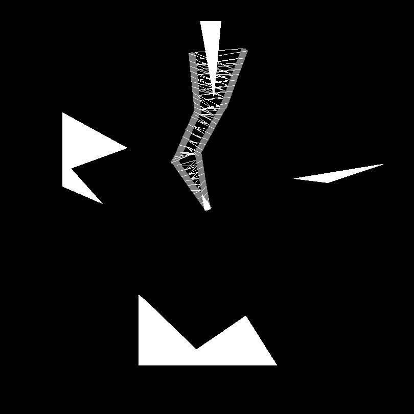
Figure 6: Interpolation in each local planner. Local planner using (a) interpolation on Local Tangent Space (LTS) (b) Ideal Tracked-Points (ITP) (c) Joins of Nearest Shi-Tomasi features link-wise (JNST).

IV-B1 Interpolation on the Local Tangent Space (LTS)

For each edge $(u,v)\in E$, let $X^{(u,v)}=\{x_{q}:q\in\mathcal{N}(u)\cap\mathcal{N}(v)\}$ be the ${p\times m}$ matrix of images corresponding to the intersection of neighbours of $u$ and neighbours of $v$ (including $u$ and $v$), where $m$ is the cardinality of $X^{(u,v)}$. To see if $(u,v)$ is safe, we interpolate the intermediate images on the tangent space spanned by $X^{(u,v)}$, obtained using PCA. The target dimension is the number of degrees of freedom $d$, and PCA maps $X^{(u,v)}$ to a $Y^{(u,v)}$ ($d\times m$). In addition to $Y^{(u,v)}$, PCA also gives a ${p\times d}$ orthonormal matrix $W^{(u,v)}$ such that $X^{(u,v)}=W^{(u,v)}Y^{(u,v)}$ or $Y^{(u,v)}=W^{(u,v)^{T}}X^{(u,v)}$. We then interpolate between $y_{u}$ and $y_{v}$ to construct $y^{(\alpha)}=\alpha*y_{u}+(1-\alpha)*y_{v}$ for various values of $\alpha\in(0,1)$. For each $\alpha$, the image $x^{(\alpha)}=Wy^{(\alpha)}$ must be in free space. In practice, the resulting image is a poor interpolation, and rejects many valid edges; however, the probability of an edge being unsafe after being passed by the local planner is low (i.e. it is conservative).

The image obtained by a linear interpolation on the local tangent space (LTS) is a weighted sum of the images in $X^{(u,v)}$. Thus, for collision detection purposes, it is sufficient to look at the superimposition of images in $X^{(u,v)}$. This achieves the same effect as the PCA based method described above, but avoids the PCA computation.

IV-B2 Ideal Tracked Points (ITP)

Here we assume that a set of points on the robot body can be tracked in all poses (including occlusions). Then to see if an edge $(u,v)$ is safe, we join each pair of corresponding tracked-points to create a new image. This image (i.e. the set of trajectories of the tracked points) are used for collision detection.

IV-B3 Join of Nearest Shi-Tomasi features (JNST)

In practice, occlusion precludes the tracking of any set of points on the robot body. Here we propose an approximation based on high-contrast points known as the Shi-Tomasi features [21]. We assume that each link of the robot can be separated and that the Shi-Tomasi features are computed on each link. Here we do not know the correspondences between points in the two images. The Join of Nearest Shi-Tomasi features approach (JNST) involves associating each feature point on each link in $u$ with the nearest feature point in the corresponding link in $v$. We do the same in both directions and insert the joins on the image.

IV-C Start and Goal states

For motion planning on the VRM, we need to map the source ($s$) and target ($t$) images onto the VRM $G$. We first ensure that the poses $s,t$ themselves are in free space. We then add these to $G$ and connect them with their $k$-nearest neighbours in $X$. We then run a local planner on the new edges and find the shortest path between $s$ and $t$ as before. Adding a new node (image) to the graph is a computation that requires $O(nk)$ distance computation steps for finding. Time for distance calculation depends on the metric used. This approach again, is almost identical to traditional roadmap methods [20], except that the tests are all visual.

V Empirical analysis : Metrics and Local Planners

Factors affecting the quality of paths in VRM include sampling density, the metric used, and the local planner. We now present an empirical study of these aspects (fig 7) on a planar 3-link simulated arm and a set of obstacles similar to those in figure 6.

V-A Gold Standard Local Planner

In the traditional Configuration Space, two configurations are assumed to be joined by a linear join between them. To see if an edge $(u,v)$ is actually safe, we generate intermediate pose images by interpolating joint angle vectors at an $\epsilon$ resolution. We observe that a linear interpolation in joint angle space need not be the same as an interpoloation on visual C-space, but we assume the difference would be fairly small for a reasonable sampling density. If all these images are collision free, we treat $(u,v)$ to be safe. The performance of the local planners is evaluated relative to this gold standard local planner. Results reported here use $\epsilon=1\degree$.

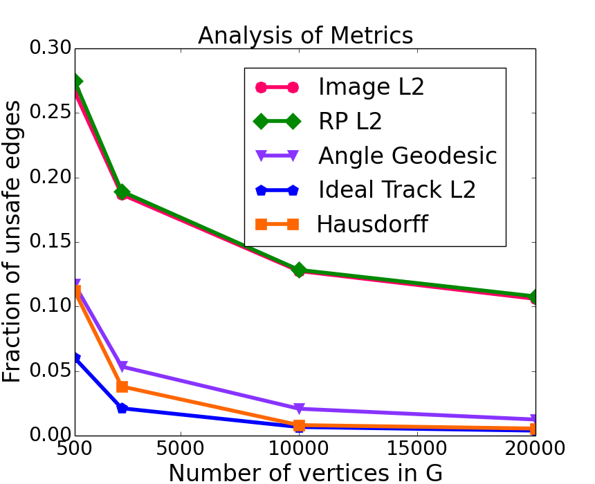
(a)

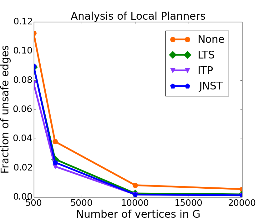
(b)

Figure 7: Empirical analysis of metrics and local planners. a) Edge failures without a local planner. b) Local planner performance plots based on Hausdorff metric. The JNST local planner performs almost as well as the ITP local planner, which is not implementable in practice.

V-B Effect of Sampling Density and Distance Metric

Plots in figure 7a clearly suggest that the sampling density (i.e., the number of images used to construct the visual roadmap) heavily affects the fraction of unsafe edges and hence the quality of paths. The more dense the sample is, the better the paths.

We present the effect of several representations of the configuration space along with appropriate distance metric for each case. Table I lists the different representations and the corresponding distance metric used to compute neighbourhoods.

TABLE I: Different representations of the configuration space and the distance metric used with each representation. Short forms mentioned here have been used in table II.

Representation	Distance Metric	Short Form
1. Raw RGB images of the robot	$L_{2}$	Img $L_{2}$
2. Random projections of images	$L_{2}$	RP $L_{2}$
3. Joint angle vector of the robot	Geodesic	$\theta$-G
4. Ideal tracked points	$L_{2}$	ITP $L_{2}$
5. Shi-Tomasi features link-wise	Hausdorff	ST-H

To find the distance between two images we just flatten all the channels of each image into a single vector and use the standard Euclidean ($L_{2}$) distance on the resulting vectors. In our experiments we used 30,000 (100x100x3) dimensional vectors for image distance.

Random projections (RP [22, 23]) is a dimensionality reduction method that preserves $L_{2}$ distances. In our experiments we projected the 30,000 dimensional image vectors onto 2000 Gaussian random unit vectors to obtain a 2000 dimensional representation of each image. The experiments show that the $L_{2}$ distance of RP vectors does almost as well as that on the image vectors. Since the distance computation is done on much smaller vectors, the graph construction gets much faster while preserving the neighbourhoods.

Distance between two joint angle vectors is computed as the sum of shortest circular-distance (i.e., treating 0 and $2\pi$ to be the same angle) between individual components. This is in some sense the geodesic distance between the two vectors.

The ideal tracked point (ITP) $L_{2}$ distance between two configurations is computed as the $L_{2}$ distance between the vectors obtained by concatenating all the tracked point coordinates of each configuration.

Finally, the Hausdorff distance between two configurations is computed as the sum of Hausdorff distances between the sets of Shi-Tomasi feature points on the corresponding links for the two configurations. Given two sets $A$ and $B$, Hausdorff distance is defined as

$$d_{H}(A,B)=max\{\sup_{a\in A}\inf_{b\in B}d(a,b),\sup_{b\in B}\inf_{a\in A}d(a,b)\}.$$

TABLE II: Percentage of bad edges remaining after pruning the VRM using each local planner on a graph with 20000 nodes with different metrics. See table I for an explanation of these metric spaces.

Local Planner	Metric Space
	Img $L_{2}$	RP $L_{2}$	$\theta$-G	ITP $L_{2}$	ST-H
None	10.59	10.79	1.25	0.39	0.55
LTS	9.18	9.34	0.43	0.09	0.19
ITP	7.97	8.11	0.17	0.11	0.12
JNST	9.58	9.74	0.16	0.12	0.12

As can be seen from figure 7b and table II, JNST local planner performs almost as well as ITP local planner.

VI Demonstrations on Real Robots

Figure 8: Path planning for the MTAB Scara robot arm. Row 1: (a),(b) some of the 4000 images of the arm. (c) scree plot. Row 2: incorporating obstacles. (a) background subtracted image of the arm, (b) image with obstacles. (c) obstacles after image subtraction. Row 3: Visual Configuration Space; obstacle nodes shown in black, and showing a path plotted from start to goal images. Row 4: path being executed by Scara.

Figure 9: Two-camera joint-manifold VRM for a 6-DOF CRS A465 robot. Since this is a 3-D workspace, obstacles cannot be distinguished from a single view. Here we use multiple cameras, and the intersection of the cones provide a (oversized) model for both obstacle and robot. To identify potential collision states, background-substracted images of the obstacle (shown in white here) are overlaid on each foreground robot image Only if the robot overlaps the obstacle in all the images, it is a potential collision node. Collision nodes shown in black.

VI-A Planar Scara robot

We now demonstrate the algorithm for a real robot, a Scara 4 DOF arm, in which two revolute joints move the first two links in a plane, so the motion has two degrees of freedom. We observe this robot with an overhead camera. 4000 images are sampled from a video while the robot is moving between random poses throughout its workspace, and the neighbourhood graph is computed. Thereafter, several obstacles are introduced in the workspace and the obstacles are discovered via background subtraction. Note that owing to the motion being planar, a single camera view is quite adequate. A planned path is shown in fig. 8.

VI-B CRS A465 robot arm

Here we have a robot in a 3-D workspace. Clearly, a single camera view will not suffice for identifying collision situations. Hence we construct a joint manifold of multiple views by stitching the corresponding images together, and constructing a joint manifold on the combined image space. The 3-DOF workspace and a path is shown in fig. 9, with the obstacle nodes marked in black.

VII Conclusion

In this work, we have introduced a new approach towards the longstanding perceptual robotics problem, which subsumes the problem of body schema learning [4, 5, 7]. Although it has been long known that there may be many kinds of generalized coordinates, so far there have been few attempts in robotics to build on this intuition. The proposed paradigm attempts to develop such a non-traditional GC, and approximates the C-space that results from it in terms of a neighbourhood graph on the set of images. We show how such a formulation for tasks such as inverse kinematic or for motion planning.

Unlike in methods used in robotics today, the Visual Generalized Coordinates approach eliminates several expensive aspects of robot modelling and planning. First, it does not require a humans to create models for robot geometry or kinematics. It does not require precise obstacle shapes and poses, and does not require to calibrate the cameras so that this can be done. There is no need for a precise simulator to test which poses collide with obstacles and which do not. Even the local planner step, based on tracking image points to nearby images, results in a more principled approach than is available presently.

Another advantage is for environments that are changing rapidly, e.g. in interaction with humans or other robots. New obstacles are updated in $O(n)$ time, but small motions by another agent require $O(m)$, where there are $m$ nodes near the obstacle boundary.

The idea of generalized coordinates originated in Lagrangian dynamics, and here is another direction that needs to be pursued. Differentiating the GC would result in generalized velocities and accelerations and this may give rise to a visual dynamics.

However, there are some significant trade-offs. First, the approach is not complete because the obstacle approximations is conservative, and there may exist paths which it cannot find. We observe that humans also face similar constraints where the vision is less informative. Secondly, it is applicable to situations where the entire C-Space is visible. While the algorithms are reasonably efficient in time complexity, the space costs are higher ($O(np)$), since all landmark images need to be stored. Another constraint is the Visual Distinguishability assumption, but this may not be very serious in practice.

The approach presented is only a beginning for discovering generalized coordinates from sensorimotor data. One of the key future steps would be to fuse modalities other than vision into a joint manifold. Thus, if we were to construct a fused visuo-motor manifold, then even if poses that are separated in motion space look similar, they would remain distinguishable. Similarly touch stimuli could be modelled to predict the result of motions or in preparation for fine-motor tasks. Such a process would also make the model more robust against noise arising in any single modality. On the whole, while the ideas presented seem promising, and open up many possibilities, much work remains to deploy Visual Generalized Coordinates fully in theory and in practice.

References

- [1] J.-C. Latombe, Robot Motion Planning, 1996.
- [2] J. B. Tenenbaum, V. de Silva, and J. C. Langford, “A global geometric framework for nonlinear dimensionality reduction,” Science, vol. 290, no. 5500, pp. 2319–2323, 2000.
- [3] J. F. Engelberger, Robotics in practice: management and applications of industrial robots. Kogan Page, 1980.
- [4] H. Poincare, “L’espace et la geometrie,” in Science and Hypothesis, 1895, pp. 60–71, transl. W. J. Greenstreet, 1905.
- [5] M. Hoffmann, H. G. Marques, A. Hernandez Arieta, H. Sumioka, M. Lungarella, and R. Pfeifer, “Body schema in robotics: a review,” Autonomous Mental Development, IEEE Transactions on, vol. 2, no. 4, pp. 304–324, 2010.
- [6] D. Pierce and B. Kuipers, “Map learning with uninterpreted sensors and effectors,” Artificial Intelligence, vol. 92, pp. 169–229, 1997.
- [7] D. Philipona, J. O’Regan, J. Nadal, and O. Coenen, “Perception of the structure of the physical world using unknown multimodal sensors and effectors,” Advances in neural information processing systems, vol. 16, 2003.
- [8] A. Arleo, F. Smeraldi, and W. Gerstner, “Cognitive navigation based on nonuniform gabor space sampling, unsupervised growing networks, and reinforcement learning,” Neural Networks, IEEE Transactions on, vol. 15, no. 3, pp. 639–652, 2004.
- [9] J. Stober, L. Fishgold, and B. Kuipers, “Sensor map discovery for developing robots,” in AAAI Fall Symposium on Manifold Learning and Its Applications, 2009.
- [10] O. Sigaud, C. Salaün, and V. Padois, “On-line regression algorithms for learning mechanical models of robots: a survey,” Robotics and Autonomous Systems, vol. 59, no. 12, pp. 1115–1129, 2011.
- [11] J. Sturm, Approaches to Probabilistic Model Learning for Mobile Manipulation Robots. Springer, 2011.
- [12] M. Kazemi, K. Gupta, and M. Mehrandezh, “Path-planning for visual servoing: a review and issues,” in Visual Servoing via Advanced Numerical Methods, 2010, pp. 189–207.
- [13] C. Von Hofsten, “An action perspective on motor development,” Trends in cognitive sciences, vol. 8, no. 6, pp. 266–272, 2004.
- [14] K. Adolph and S. Berger, “Motor development,” in Handbook of child psychology, 2006.
- [15] J. Stening, H. Jacobsson, and T. Ziemke, “Imagination and abstraction of sensorimotor flow: Towards a robot model,” in Proceedings of the AISB05 Symposium on Next Generation approaches to Machine Consciousness: Imagination, Development, Intersubjectivity, and Embodiment, 2005, pp. 50–58.
- [16] S. M. LaValle, Planning Algorithms. Cambridge, U.K.: Cambridge University Press, 2006, available at http://planning.cs.uiuc.edu/.
- [17] L. E. Kavraki, P. Švestka, J.-C. Latombe, and M. H. Overmars, “Probabilistic roadmaps for path planning in high-dimensional configuration spaces,” Robotics and Automation, IEEE Transactions on, vol. 12, no. 4, pp. 566–580, 1996.
- [18] N. Kambhatla and T. K. Leen, “Dimension reduction by local principal component analysis,” Neural Computation, vol. 9, no. 7, pp. 1493–1516, 1997.
- [19] J. Yang, F. Li, and J. Wang, “A better scaled local tangent space alignment algorithm,” in Neural Networks, 2005. IJCNN’05. Proceedings. 2005 IEEE International Joint Conference on, vol. 2, 2005, pp. 1006–1011.
- [20] H. Choset, K. M. Lynch, S. Hutchinson, G. A. Kantor, W. Burgard, L. E. Kavraki, and S. Thrun, Principles of Robot Motion: Theory, Algorithms, and Implementations. Cambridge, MA: MIT Press, June 2005.
- [21] J. Shi and C. Tomasi, “Good features to track,” in 1994 IEEE Conference on Computer Vision and Pattern Recognition (CVPR’94), 1994, pp. 593 – 600.
- [22] E. Bingham and H. Mannila, “Random projection in dimensionality reduction: applications to image and text data,” in Proceedings of the seventh ACM SIGKDD international conference on Knowledge discovery and data mining. ACM, 2001, pp. 245–250.
- [23] S. Dasgupta, “Experiments with random projection,” in Proceedings of the Sixteenth conference on Uncertainty in artificial intelligence. Morgan Kaufmann Publishers Inc., 2000, pp. 143–151.