A quantum chemical study from a molecular perspective: ionization and electron attachment energies for species often used to fabricate single-molecule junctions

Ioan Bâldea ^{∗ a‡}

Published: Faraday Discussions 2014, 174, 37-56; DOI: 10.1039/C4FD00101J

Abstract:
The accurate determination of the lowest electron attachment ($EA$) and ionization ($IP$) energies for molecules embedded in molecular junctions is important for correctly estimating, e.g., the magnitude of the currents ($I$) or the biases ($V$) where an $I-V$-curve exhibits a significant non-Ohmic behavior. Benchmark calculations for the lowest electron attachment and ionization energies of several typical molecules utilized to fabricate single-molecule junctions characterized by n-type conduction (4,4’-bipyridine, 1,4-dicyanobenzene, and 4,4’-dicyano-1,1’-biphenyl) and p-type conduction (benzenedithiol, biphenyldithiol, hexanemonothiol, and hexanedithiol] based on the EOM-CCSD (equation-of-motion coupled-cluster singles and doubles) state-of-the-art method of quantum chemistry are presented. They indicate significant differences from the results obtained within current approaches to molecular transport. The present study emphasizes that, in addition to a reliable quantum chemical method, basis sets much better than the ubiquitous double-zeta set employed for transport calculations are needed. The latter is a particularly critical issue for correctly determining $EA$’s, which is impossible without including sufficient diffuse basis functions. The spatial distribution of the dominant molecular orbitals (MO’s) is another important issue, on which the present study draws attention, because it sensitively affects the MO-energy shifts $\Phi$ due to image charges formed in electrodes. The present results cannot substantiate the common assumption of a point-like MO midway between electrodes, which substantially affects the actual $\Phi$-values.

Keywords: molecular electronics, single-molecule junctions, quantum chemical calculations, electron attachment, ionization

1 Introduction

Electron or hole injection into molecules embedded between two electrodes represents an important issue in the fabrication of molecular devices. The efficiency of the charge injection and transport in molecular junctions is controlled by the highest occupied or lowest unoccupied molecular orbital (HOMO or LUMO, respectively), whichever is closest to the electrodes’ Fermi energy $E_{F}$, and the key quantity is the energy offset $\varepsilon_{0}=\min(E_{F}-E_{HOMO},E_{LUMO}-E_{F})$. It can be compared to a tunneling barrier, which charge carriers have to overcome to generate a current. Ultraviolet photoelectron spectroscopy (UPS) ¹, thermopower ^{2, 3, 4}, and transition voltage spectroscopy (TVS) ^{5, 6, 7, 8, 9, 10} represent current methods to estimate the relative alignment of the dominant molecular orbital from experimental data.

Recent analysis of a variety of transport data demonstrated that full current-voltage $I-V$ curves beyond the ohmic regime can be quantitatively reproduced by assuming that molecular transport is dominated by a single level (to be identified with HOMO or LUMO) ^{7, 11, 12, 9, 13, 14}. This is an enormous simplification. Still, the correct description of the relative alignment $\varepsilon_{0}$ ($=E_{LUMO}-E_{F}$ or $E_{F}-E_{HOMO}$) remains an important challenge for ab initio approaches to the charge transport through single-molecule junctions. It is a challenge particularly because of the high accuracy needed. Values directly determined in ultraviolet photoelectron spectroscopy (UPS) experiments amount to $\varepsilon_{0}\sim 1$ eV ¹. Results based on TVS by using a model able to excellently reproduce current-voltage ($I-V$) curves measured in single-molecule junctions demonstrate that $\varepsilon_{0}$ can be even smaller ($\varepsilon_{0}\simeq 0.6$ eV ¹³). It should be clear that, in view of such low-$\varepsilon_{0}$ values, estimates for $IP$’s and $EA$’s with errors $\simeq$0.5 eV typical for quantum chemical methods of moderate accuracy are unacceptable. Noteworthy, the quantity $\varepsilon_{0}$ is important not only because it determines the magnitude of the currents, but also because it indicates the biases beyond which an $I-V$ curve becomes significantly nonlinear ¹².

An important message, which the present study aims to convey, is that the accurate determination of the HOMO and LUMO energies (or, more precisely, the lowest ionization $IP$ and electroaffinity $EA$ with reversed sign) represent a nontrivial issue even for isolated species of interest for molecular transport. Obviously, this is a minimal requirement for any molecular transport approach.

In the present paper we report results of ongoing work focusing on several prototypical molecular species, which are mostly utilized in the fabrication of single-molecule junctions, and examine the reliability of the results for ionization energies $IP$($\approx-E_{HOMO}$) and electroaffinities $EA$($\approx-E_{LUMO}$) as obtained within current methods employed in molecular transport with accurate estimates obtained within well-established quantum chemical methods. To avoid misunderstandings, let us explicitly mention that we will restrict ourselves throughout to the lowest $IP$ and $EA$; in fact, if at all, for the molecules analyzed below it is only the lowest $EA$ that corresponds to a stable anion ($EA>0$).

The molecular species to be considered will include, besides 4,4’-bipyridine (44BPY) — a molecule recently considered from a TVS perspective ^{13, 15} —, molecules often used to fabricate two classes of molecular junctions. One class is represented by molecules characterized by n-type (LUMO-mediated) conduction, the other class comprises molecules characterized by p-type (HOMO-mediated) conduction. As specific examples belonging to the first class, we will consider 44BPY ³, BDCN (1,4-dicyanobenzene) ¹⁶, and 2BDCN (4,4’-dicyano-1,1’-biphenyl). From the second class, we will examine oligophenylene dithiols ^{8, 4} and alkanemono- and dithiols ¹⁷.

Because of well-documented shortcomings of ubiquitous methods based on density functional theory (DFT), emphasis will be on post-DFT methods. Besides methods already utilized in approaches to molecular transport (e.g., $\Delta$-SCF ¹⁸, $GW$ ¹⁹ and MP2 ²⁰), we will consider truly ab initio methods used in quantum chemistry: outer valence Green’s functions (OVGF) ^{21, 22}, second-order algrabraic-diagrammatic constructions [ADC(2)] ^{23, 24}, and equation-of-motion (EOM) coupled-cluster (CC) ²⁵ approaches. The importance of using appropriate quantum chemical methods will be emphasized. As is well known, calculating $EA$’s is a very delicate problem in quantum chemistry altogether ²⁶.

2 Methods

Active molecules embedded in molecular junctions can be treated at various levels of theory ranging from tight-binding (extended Hückel) to and post-DFT. In order to facilitate understanding the message, which the results reported below aim to convey, we will briefly present the methods utilized in this study.

(i) If the picture based on the self-consistent field (SCF) were valid (or, equivalently, electron correlations were absent), the energy of highest occupied Hartree-Fock (HF) orbital (i.e., HOMO) with reversed sign would represent the lowest ionization energy $IP=-E_{SCF,HOMO}$ (Koopmans theorem). The physical meaning of the virtual (unoccupied) is controversial ^{27, 28}. Virtual HF orbitals might have physical meaning if descriptions based on small basis sets succeeded (at least semi-)quantitatively, but this is often not the case. Table 8 illustrates this failure, where results relevant in connection with existing MP2-based transport approaches and minimal (STO-6G) basis sets ²⁹ are presented. At the other extreme, it is also well known that the HF LUMO energy goes to zero in the complete basis set limit ^{30, 31}. This is a reason why attempts to “improve” the quality of a transport approach by using larger and larger basis sets end up with unphysical results ³². For large atomic orbital (AO) basis sets, the virtual HF orbitals have mathematical rather than physical meaning, namely, in providing an expansion manifold for the physical states of interest. In some cases, individual virtual or unoccupied HF orbitals (in particular, the LUMO) can reasonably describe, e.g., anionic bound or resonance states semi-quantitatively, provided that the size of the AO basis used is not too large ¹³.

(ii) Within DFT-approaches, the single particle solutions of the Kohn-Sham (KS) equations are handled as if the corresponding eigenvalues/eigenfunctions were real orbital energies/wave functions. The corresponding implementation in a Landauer-NEGF formalism is straightforward because the DFT description is mathematically a single-particle description. This is why the DFT approaches to molecular transport are by far the most popular to date. Drawbacks of such DFT-approaches are well documented. The drastic underestimation of the HOMO-LUMO gap and the related lineup problem (HOMO/LUMO energies too close to electrodes’ Fermi energy) are issues most frequently mentioned and not at all surprising: as is well known ¹⁸, KS “orbitals” are mathematical objects rather than physical orbitals.

The quantum chemical methods used in the present paper to compute the lowest electroaffinity ($EA$) and ionization $IP$ energies are:

(iii) The outer valence Green’s function (OVGF) method ^{33, 22} represents the most elaborate quantum chemical approach based on a single-particle picture. To the best of our knowledge, the OVFG approach has not yet been utilized in molecular transport studies. Therefore, let us mention that the OVGF method is a way to approximately include the contribution of the electron-electron interaction beyond HF. Details can be found in ref. ^{33, 22}. As explained below, this method is superior to the MP2-like approximation used recently ²⁰ (see sec. 4.3). The OVGF method ^{33, 22} exactly treats the full second- and third-order terms in the self-energy entering the Dyson equation for the one-electron Green function, and is augmented by a geometrical approximation to also include further higher-order corrections ³⁴. Results for the electron affinities and ionization energies obtained by considering the second- and third-order terms are shown in the tables presented below (they are labeled as “2nd-order pole” and “3rd-order pole”, respectively) along with those of the full OVGF. The corresponding pole strengths ²² are also indicated (percents in parentheses).

(iv) The algebraic-diagrammatic construction (ADC) is based on a diagrammatic perturbation expansion. ADC(n) defines an approximate scheme of infinite partial summations exact up to the $n$-th order of perturbation theory ^{23, 24}. Its second-order version ADC(2) is superior to the so-called $GW$-approximation ¹⁹, since only bubble contributions are included within the $GW$ and not all second-order terms: expressing the self-energy $\boldsymbol{\Sigma}$ by the product of the single-electron Green’s function $\boldsymbol{G}$ and the effective interaction $\boldsymbol{W}$ ($\boldsymbol{\Sigma}\sim\boldsymbol{GW}$, thence the name $GW$), vertex corrections ³⁵ are neglected within $GW$.

(iv) Equation-of-motion (EOM) coupled-cluster (CC) approaches at singles and doubles (CCSD) ³⁶, hybrid (CC2) ³⁷, and perturbative [CCSD(2)] ^{38, 39} levels will be extensively applied in this paper. Corrections due to triples [EOM-CCSD(T)] will be also considered; the fact that these corrections are altogether negligible is an indication on the accuracy of the state-of-the-art EOM-CCSD method.

(vi) Energy difference ($\Delta$-) methods will be utilized for all the aforementioned cases. Within these methods, the lowest ionization energy $IP$ and electron affinity $EA$ are estimated as differences between the ground state energies $\mathcal{E}$ of the corresponding molecular charge species ($M$=SCF, DFT, MP2, CCSD, CC2) at the equilibrium geometry of the neutral molecule

$$IP\to\Delta_{M}^{i} = \mathcal{E}_{M,cation}-\mathcal{E}_{M,neutral},$$ (1)

$$EA\to\Delta_{M}^{a} = \mathcal{E}_{M,neutral}-\mathcal{E}_{M,anion}.$$ (2)

3 Computational details

The results of the SCF, DFT/B3LYP, MP2, and OVGF calculations reported below were done with GAUSSIAN 09 ⁴⁰. Coupled-cluster calculations of the $IP$, $EA$, total energies of the various charge species and excitation energies were performed with CFOUR ⁴¹. Calculations within the so-called regular (strict) ADC(2) reported here have been done with the fully parallelized PRICD-$\Sigma$(2) code ⁴², which is interfaced to MOLCAS ⁴³. As amply documented by extensive work of the Heidelberg theoretical chemistry group, the results based on the strict ADC(2) are comparable to the second-order approximate coupled cluster singles and doubles model (CC2) ³⁷. Augmented with extra terms in an extended version [ADC(2)x] ⁴⁴, the results become comparable to the equation of motion coupled cluster singles and doubles method (EOM-CCSD) ³⁶. Unfortunately, a code enabling computations for molecular sizes of interest for molecular transport is not (yet) available.

The inspection of the tables presented below reveals that the results obtained via the state-of-the-art IP- and EA-EOM-CCSD method ^{45, 36} and aug-cc-pVDZ (Dunning augmented correlation consistent double zeta) sets can be trusted. This is illustrated both by the good agreement between the EOM-CCSD and the $\Delta$-CCSD values and by the fact that corrections due to triples [CCSD(T)] yield changes that are irrelevant within numerical errors. For understanding the impact of polarization and diffuse functions we also present results obtained by using other basis sets: cc-pVDZ and cc-pVTZ, Pople basis sets (6-31G*, 6-311G* 6-311++G(d,p)), Dunning-Huzinaga double- and triple-zeta (DZ (DZ95 in ref. ⁴⁰), DZP, TZ2P), Karlsruhe basis sets (svp, dzp, tzp, qz2p), and (merely to compare with earlier MP2-based transport calculations, cf. Table 8) STO-6G.

4 Results and discussion

Because the tables presented in this paper, which contain very detailed information on both the methods and the basis sets employed, are self-explanatory, below we will only briefly emphasize the main aspects related to the lowest electron attachment ($EA$) and ionization ($IP$) energies of the molecules of interest. Still, as a technical remark, let us mention that, in view of the fact that double zeta (DZ) sets are ubiquitous in transport studies, among other basis sets, we have always included DZ-based results in the relevant tables.

4.1 Lowest electron attachment energies

Table 1, 2, and 3 collect results on the lowest electron attachment energies for 4,4’-bipyridine (C6H4N₂, 44BPY), 1,4-dicyanobenzene (NC-C6H4-CN, BDCN), and 4,4’-dicyano-1,1’-biphenyl (NC-(C6H4)2-CN, 2BDCN).

Table 1 presents very detailed numerical results for 44BPY, a showcase molecule ^{46, 47, 13, 15, 48}, in order to illustrate the main issues, which we have encountered in calculations of electroaffinities for molecules utilized in molecular electronics. The EA-EOM-CCSD method predicts a weakly bound anion 44BPY^∙- ($EA\raisebox{-1.29167pt}{$\stackrel{{\scriptstyle>}}{{\sim}}$}0$). The essential condition for this is the inclusion of a sufficient number of diffuse basis functions. As emphasized recently ⁴⁷, it is not the basis set size that matters: as visible in Table 1, the basis set CC-pVTZ, which is larger than aug-cc-pVDZ, cannot stabilize the anion, just because diffuse functions are missing.

Notice also that a correct description requires a proper treatment of electron correlations. Even including sufficient diffuse basis functions (aug-cc-pVDZ), the SCF description (both Koopmans theorem and $\Delta$-SCF) is even qualitatively inadequate; the anion is predicted to be unstable. This is already known from earlier work ^{49, 50, 47}. As visible in Table 1, we found that electron correlations (which, by definition, measure deviation from SCF) cannot be adequately included via MP2 and the OVGF ^{21, 22}: the 44BPY^∙- anion remains unstable.

On the other side, while agreeing among themselves, the CC2, ADC(2), and $\Delta$-DFT all overestimate the anion stability. Concerning CC2, one can remark that $\Delta$-CC2 performs better than EOM-CC2.

Basically, the conclusions formulated above by analyzing the electron affinity of 44BPY also holds for the other two molecules [1,4-dicyanobenzene (BDCN) and 4,4’-dicyano-1,1’-biphenyl (2BDCN)] investigated; see Table 2 and 3. Quantitatively, there is an important difference: the BDCN^∙- and 2BDCN^∙- anions are substantially more stable: their electroaffinities are by about $0.7$ eV larger than that of the 44BPY^∙- anion.

To summarize, the anions considered above can be accurately described at the CCSD level of theory provided that the basis set employed includes sufficient diffuse functions: triplet corrections [i.e., CCSD(T)] merely yield modifications of the EA-values within numerical errors, and the EA-EOM-CCSD values agree well with the $\Delta$-CCSD values.

4.2 Lowest ionization energies

As representatives of molecules embedded in nanojunctions exhibiting a HOMO-mediated (p-type) conduction, we have studied and present detailed results for benzenedithiol (HS-C6H4-SH, BDT, Table 4) and related molecules (S-C6H4-S and S-C6H3F-S, Table 8), dibenzenedithiol (HS-(C6H4)2-SH, 2BDT, Table 5), 1,6-hexanemonothiol (H-(CH2)6-SH, C6MT, Table 6), and 1,6-hexanedithiol (HS-(CH2)6-SH, C6DT, Table 7).

As visible in these tables, the lowest ionization energies can be estimated with a good relative accuracy ($\raisebox{-1.29167pt}{$\stackrel{{\scriptstyle<}}{{\sim}}$}4\%$), which is satisfactory for quantum chemical calculations for many purposes, within IP-EOM-CCSD calculations by using rather modest basis sets. Although not dramatically large, the corresponding absolute error ($\raisebox{-1.29167pt}{$\stackrel{{\scriptstyle<}}{{\sim}}$}0.4$ eV) is still non-negligible from a molecular transport perspective in view of the rather small energy offset of the dominant molecular orbital relative to electrodes’ Fermi level. So, good basis sets are required not only for $EA$’s, but also for an adequate $IP$’s. Even for cations, the various lower level many-body approximations (MP2, CC2, ADC(2), CCSD(2) as well as their $\Delta$-versions), deviating by up to $\sim 0.4$ eV from the EOM-CCSD approach, are still not too satisfactory.

In view of the present results, the $\Delta$-DFT method cannot be recommended: deviations from the $IP$-EOM-CCSD estimate can be very large; the example presented in Table 7 indicates an error of $\sim 0.8$ eV.

A special mention deserves the OVGF approximation, which appears to provide the $IP$-estimates closest to EOM-CCSD; the differences are smaller than $0.1$ eV.

4.3 Comparison with results of previously utilized many-body methods

The foregoing analysis drew attention that both the quantum chemical method and the basis set utilized are important for correct $EA$- and $IP$-estimations. Employing small basis sets is particularly tempting for truly ab initio approaches, which are otherwise impracticable, as they require much more RAM-memory, disc space, and computational time than ubiquitous DFT-flavors.

In this subsection, we will scrutinize the reliability of the results obtained by post-DFT approaches reported in two earlier studies ^{29, 51}. To assess the validity of those methods, we will present a comparison with results of the present methods also using the same small basis sets of ref.  ^{29, 51}.

Ref. ²⁹ reported results obtained within an MP2-like approach for two molecules, namely (S-C6H4-S and S-C6H3F-S), which are similar to BDT(=HS-C6H4-SH). In Table 8, we present results for these molecules obtained within the methods described above along with those extracted from ref. ²⁹. Following ref. ²⁹, we refer to the latter results as “MP2-based”. Still, for clarity, we should note that, in the present terminology, the method of ref. ²⁹ coincides with that labeled “2nd-order pole” here, as it corresponds to the second-order correction in the the electron-electron interaction to the electronic self-energy ^{21, 22}. So, the results labeled “MP2-based” and “2nd-order pole” in Table 8 should coincide. They should but they do not coincide; or, more precisely, they are substantially different. We cannot understand these large differences ($\raisebox{-1.29167pt}{$\stackrel{{\scriptstyle>}}{{\sim}}$}1$ eV) visible in Table 8. The only thing not specified in ref. ²⁹ is the molecular geometry utilized in the calculations. However, as actually expected, the results presented in Table 8 reveal that differences in (optimized) geometries have a considerable smaller impact (maybe $\sim 0.2$ eV). Most importantly, as seen in Table 8, it is the combined effect of an inaccurate method and a too small basis set that results in very large errors ($\sim 3$ eV) for $IP$’s.

By using the same (DZ) basis sets as in ref. ⁵¹, Table 9 demonstrates that the results deduced within the $GW$ method are not adequate to estimate the energies of the frontier orbitals with the accuracy required for molecular transport studies. Differences $\sim 0.5$ eV between the $GW$ and EOM-CCSD visible in Table 9 are too large, given the fact that for this molecule (BDT) the HOMO energy offset directly measured by ultraviolet photoelectron spectroscopy (UPS) amounts to $\simeq 1$ eV ¹. Drawbacks of $GW$-based transport approaches were previously pointed out ⁵².

4.4 Spatial distribution of the frontier molecular orbitals

As highlighted above, both the method and the basis sets employed are essential to properly estimate the energy of the frontier orbitals of an isolated molecule. Still, however important, the level energy of an isolated molecule is not the whole issue. In a molecular junction, the active molecule is linked to electrodes, which yield shifts in energy via image charge effects. This effect, which is well established in surface science ⁵³, was embodied in recent studies on molecular electronics in a simplified form, namely by assuming point-like molecular orbitals midway between electrodes ^{54, 3}. This assumption is indeed a comfortable approximation, as it can readily be implemented in one-shot DFT+$\Sigma$ transport calculations ^{55, 3}.

The obvious critical point here, on which ref. ¹³ has recently drawn attention, is to what extent is it legitimate to approximate a real molecular orbital as a point charge. Within classical electrostatics, the interaction energy of an electron located at $z$ with the image charges created in two infinite planar electrodes can be exactly expressed by ^{56, 57}

$$\phi_{i}(z)=\frac{e^{2}}{4d}\left[-2\psi(1)+\psi\left(\frac{z-z_{s}}{d}\right)+\psi\left(\frac{z_{t}-z}{d}\right)\right].$$ (3)

Here, $z_{s,t}$ are the positions of the image planes (which are slightly shifted from the real electrodes, see, e.g, ref. ¹³ and citations therein), $d\equiv z_{t}-z_{s}$, and $\psi(z)\equiv d\,\log\Gamma(z)/d\,z$ is the digamma function. For a real molecular orbital, the image-driven energy shift should be computed by weighting eqn (3) with the MO-spatial density $\rho_{MO}=|\Psi_{MO}|^{2}$, which is determined by its wave function $\Psi_{MO}$

$$\Phi=\int_{z_{s}}^{z_{t}}d\,z\,\rho_{1D}^{MO}(z)\,\phi_{i}(z),$$ (4)

$$\rho_{1D}^{MO}(z)=\int\int d\,x\,d\,y\,|\Psi_{MO}(x,y,z)|^{2}.$$ (5)

Close to electrodes, e. g., $z\raisebox{-1.29167pt}{$\stackrel{{\scriptstyle>}}{{\sim}}$}z_{s}$, eqn (3) recovers the classical expression

$${\phi}_{i}(z){\raisebox{-1.29167pt}{$\stackrel{{\scriptstyle z\raisebox{-0.90417pt}{\raisebox{-0.90417pt}{$\stackrel{{\scriptstyle>}}{{\sim}}$}}z_{s}}}{{\approx}}$}}\phi_{i,cl}(z)=-\frac{e^{2}}{4(z-z_{s})}$$ (6)

for a single image plane. This demonstrates that, in cases of molecular orbitals with significant spatial extension, the main contributions to the image-driven energy shift $\Phi$ come from regions close to electrodes.

Since, except for ref. ¹³, the spatial extension of the dominant molecular orbitals did not received consideration in previous studies, we have decided to systematically investigate this aspect for typical molecules of interest for nanotransport. To this aim, inspecting spatial densities of (completely unphysical LUMO) Kohn-Sham orbitals makes little sense, and (especially LUMO) HF orbitals may represent a too crude approximation. Therefore, like in ref. ²⁶, we have calculated the natural orbital expansion of the corresponding reduced density matrices at the EOM-CCSD level.

This is the most reliable approach to characterize the spatial distribution of the extra electron or hole in molecules with n-type (LUMO-mediated) or p-type (HOMO-mediated) conduction, and we are not aware of a similar study conducted in conjunction with molecular transport at this level of theory. For all the molecules considered, by inspecting the natural orbital expansion, we found that the extra electron or hole is almost entirely ($>97\%$) concentrated in a single natural orbital.

Most importantly from the present standpoint, we found not even a molecule whose dominant MO reside in a very narrow spatial region around the center.

Rather than being strongly localized close to the center, in cases of n-conduction, we found that the natural orbital of the extra electron is more or less uniformly spread over the whole molecule. This is illustrated by the examples depicted in Fig. 1 and 2.

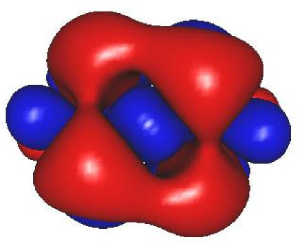
Fig.  1: The almost singly occupied natural orbital corresponding to the anion’s extra electron of the 44BPY^∙- anion (“LUMO”) obtained via EA-EOM-CCSD/aug-cc-pVDZ calculations is delocalized over the whole molecule.

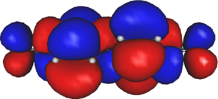
Fig.  2: The almost singly occupied natural orbital of the extra electron in the 2BDCN anion (“LUMO”) is delocalized over the whole molecule. Result of EA-EOM-CCSD/aug-cc-pVDZ calculations.

(We employed Gabedit ⁵⁸ to generate the figures presented in this paper.) Therefore, the difference between the value $\Phi_{loc}=-e^{2}\ln 2/d$ obtained by setting $z=(z_{s}+z_{t})/2$ in eqn (3), which corresponds to a point-like MO located in the middle of two infinite metallic plates ³, is substantially different from the value $\Phi_{r}$ deduced via eqn (4) by using the realistic natural orbital density. For the 44BPY molecule, the values thus obtained for the image-driven LUMO shifts are $\Phi_{r}=-2.13$ eV and $\Phi_{loc}=-1.16$ eV. A difference of about 1 eV is a big effect.

We have also computed spatial distributions of the natural orbital of the extra hole (“HOMO”) in cation species relevant for molecules exhibiting p-type conduction. The examples presented in Fig. 3 and 4 illustrate two different behaviors, which we found to be characteristic for HOMO distributions.

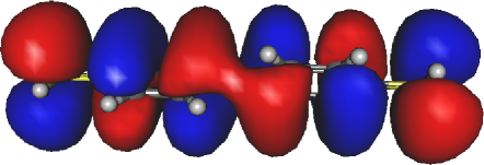
Fig.  3: The almost singly occupied natural orbital of the extra hole (“HOMO”) in the BDT cation is delocalized over the whole molecule. Result of IP-EOM-CCSD/aug-cc-pVDZ calculations.

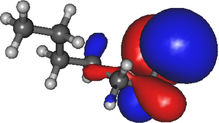
Fig.  4: The almost singly occupied natural orbital of the extra hole (“HOMO”) in the hexanemonothiol cation is localized in the vicinity of the sulfur atom. Result of IP-EOM-CCSD/aug-cc-pVDZ calculations.

On one side, we found HOMO’s like that presented in Fig. 3, which are similar to the LUMO’s discussed above; they are delocalized over the whole molecule. On the other side, we found HOMO’s strongly localized on the anchoring groups. Typical for this behavior are alkanemono- and dithiols, as illustrated in Fig. 4

To obtain the above value $\Phi_{r}$($=-2.16$ eV) for 44BPY, we applied the cutoff procedure near electrodes described in detail in ref. ¹³. Results of preliminary calculations with metal atoms linked to the molecules with LUMO-mediated conduction considered here indicate that, like the case of ref. ¹³, the spatial density LUMO (single occupied natural orbital corresponding to the extra electron) does not substantially penetrate into electrodes. This is important: corrections due to image charges are not dramatically affected by the cutoff procedure close to electrodes. This behavior contrasts to that of the HOMO’s. Whether delocalized (like that of Fig. 3) or localized (like that from Fig. 4) on the terminal groups of the isolated molecules, we found that the HOMO distributions substantially penetrates into electrodes. Although we only checked that this happens for molecules of the types discussed above, we believe that this is a general HOMO property that ensures stable molecule-electrode bonds. A cutoff procedure is needed to eliminate spurious divergences of the classical expression of the interaction energy with image charges at $z=z_{s,t}$ [cf. eqn (3) and (6)], which ignores quantum mechanical effects and electrodes’ atomistic structure. A possible cutoff procedure consists of multiplying the classical expression with factors $1-\exp(-\mu|z-z_{s,t})$ ($\propto|z-z_{s,t}|$ as $z\to z_{s,t}$); see, e.g, ref. ¹³ and citations therein. Cutoff procedures make sense only if the results do not sensitively depend on the value of cutoff parameter $\mu$, and this cannot be the case if (HO)MO densities have non-negligible values in spatial regions close to electrodes ($z\sim z_{s,t}$).

4.5 The exciton binding energy as evidence for important electron correlations

As a possible way to quantify electron correlations, the solid-state community employs the difference between the so-called charge gap $\Delta_{c}$ and the optical gap(=lowest excitation energy) $\Delta_{o}$; see e.g. ref. ^{59, 46} and citations therein. The charge gap, which is what molecular physicists normally call the HOMO-LUMO gap, can be expressed as $\Delta_{c}=IP-EA$. Loosely speaking [because in reality the single-particle (MO) picture breaks down in the exciton problem], the difference between the charge gap and the optical gap is that, in determining $EA$, both HOMO and LUMO are occupied. By contrast, in the lowest optical excitation, the HOMO becomes empty as the LUMO becomes occupied. $\Delta_{c}$ should be larger than $\Delta_{o}$ because of the (negative) attraction energy between the oppositely charged electron (LUMO) and hole (HOMO) This difference is referred to as the exciton binding energy $EBE$ (see, e.g., ref. ³⁵)

$$EBE=\Delta_{c}-\Delta_{o}.$$ (7)

The various tables of the present paper only include results for $EBE$ obtained within the most accurate method utilized (EOM-CCSD). The $EBE$-values shown there are substantial, amounting to up to $\sim 50\%$ of the charge gap. As expected for molecules with aromatic units and delocalized electrons, the $EBE$ decreases with increasing molecular size; compare the $EBE$-values for BDCN (Table 2) and 2BDCN (Table 3), and for BDT (Table 4) and 2BDT (Table 5). The $EBE$-values ($EBE\sim 3.5-4.6$ eV) estimated for all the molecules analyzed in the present paper are substantially larger than, e.g., for $\pi$-conjugated organic thin films ($EBE\sim 0.6-1.4$ eV) ⁶⁰.

So, one should conclude that, for species of interest for molecular electronics, electron correlations are very strong. This aspect may be quite relevant for developing correlated transport approaches ⁶¹; e.g., even if the charge transport is dominated by the LUMO, an electron traveling through the molecule can interact with the HOMO.

5 Conclusion

In this paper, we have presented benchmark quantum chemical calculations for the lowest electron attachment and ionization energies of several isolated molecular species of interest for molecular electronics. In assessing the importance of the accuracy to be achieved by estimating $EA$’s and $IP$’s, it is worth mentioning that a proper understanding of the charge transport at nanoscale does not only mean to reproduce the (order of) magnitude of the currents (which can be adjusted by “manipulating” both $\varepsilon_{0}$ and the broadening functions $\Gamma$ not considered here), but also the biases $V$ characterizing a non-Ohmic regime, which is basically determined by $\varepsilon_{0}$ ($eV~{}\varepsilon_{0}$, see ¹²).

The main results presented above can be summarized as follows:

(i) For all molecules, the differences between the HF-MO energy (Koopmans theorem) and $\Delta$-SCF values are large. This demonstrates that orbital relaxation is substantial. Electron correlations are also important, as revealed by important departures from the SCF results as well as by substantial differences between the various post-SCF methods considered.

(ii) The present results demonstrate the need both for accurate methods and good basis sets beyond those currently utilized in transport approaches. In particular, employing basis sets with sufficient diffuse functions is essential to correctly describe electron affinities.

(iii) Kohn-Sham orbital energies can by no means be used to estimate $IP$’s and $EA$’s. Even with $\Delta$-corrections, DFT-based methods do not appear to achieve the desired accuracy of estimating the relevant MO energy offsets $\varepsilon_{0}$. As visible in the various tables, because $\Delta$-DFT estimates are much weakly dependent on the basis sets that those of EOM-CCSD; so, $\Delta$-DFT may convey a false impression on the importance of the basis sets to be utilized in calculations.

(iv) MP2-based methods appear to be completely inadequate for describing anions. For cations, they may yield substantially different results; e.g., compare the deduced via $\Delta$-MP2 and the second-order order correction to self-energy (“2nd-order pole) ($>1.6$ eV in Table 5). Examples showing that different methods to include second-order terms in the electron-electron interaction in other contexts were discussed earlier ⁶².

(v) For the presently investigated molecules exhibiting p-type conduction, the OVGF method represents an excellent compromise in terms of computational effort and accuracy of $IP$-estimates. Unlike the other diagrammatic methods considered here ($GW$ and $ADC$), the OVGF method does not require to self-consistently solve a(n integral) Dyson equation; the electron self-energy $\boldsymbol{\Sigma}(\varepsilon)$ can be expressed in closed analytical form, and what needs to solve is a nonlinear algebraic equation for $\varepsilon$ ²². To be fair, let us also mention that, for the presently considered molecules that form junctions characterized by n-type conduction, the OVGF method turned out to be totally inadequate.

(vi) The spatial distribution of the frontier orbitals plays an important role to reliably estimate image-driven shifts of the relevant MO-energies. To the best of our knowledge, this is the first systematic study on the spatial distribution of the extra electron or hole in molecular species of interest for molecular transport at this (EOM-CCSD natural orbital expansion) level of theory. None of the molecules considered in this paper was found to possess point-like frontier molecular orbitals, a fact that contradicts the common assumption made in the field.

Acknowledgments  

The author thanks Shachar Klaiman and Evgeniy Gromov for invaluable help to perform quantum chemical calculations, and Jochen Schirmer for useful discussions. Thanks are also due to Vitja Vysotskiy, whose fully parallelized PRICD-$\Sigma$(2) code has been employed to obtain the ADC(2) results for electron affinity and ionization energies reported here. Calculations for this work have been partially done on the high performance bwGrid cluster ⁶³. Financial support from the Deutsche Forschungsgemeinschaft (grant BA 1799/2-1) is gratefully acknowledged.

44BPY/Method	Basis set	No. functions	$EA$ (eV)	$EBE$ (eV)
EOM-CCSD	DZ	136	-0.684
EOM-CCSD	6-31G**	208	-0.686
EOM-CCSD	svp	208	-0.421
EOM-CCSD	cc-pVDZ	208	-0.484
EOM-CCSD	dzp	220	-0.353
EOM-CCSD	6-311G**	264	-0.340
EOM-CCSD	tzp	276	-0.290
EOM-CCSD	TZ2P	360	-0.0247
EOM-CCSD	qz2p	416	-0.0123
EOM-CCSD	cc-pVTZ	472	-0.438
EOM-CCSD	aug-cc-pVDZ	348	0.0322	4.487
EOM-CCSD(T)	aug-cc-pVDZ	348	0.0293
EOM-CC2	aug-cc-pVDZ	348	0.360
ADC(2)	aug-cc-pVDZ	348	0.370
$\Delta$-SCF	aug-cc-pVDZ	348	-0.564
$\Delta$-MP2	aug-cc-pVDZ	348	-0.500
$\Delta$-CCSD	aug-cc-pVDZ	348	0.0043
$\Delta$-DFT/B3LYP	DZ	136	0.185
$\Delta$-DFT	6-31G*	196	-0.126
$\Delta$-DFT/B3LYP	svp	208	0.124
$\Delta$-DFT	6-31G**	208	-0.115
$\Delta$-DFT	cc-pVDZ	208	0.0290
$\Delta$-DFT	6-31+G(d)	244	0.396
$\Delta$-DFT	6-311G**	264	0.188
$\Delta$-DFT	6-31+G(d,p)	268	0.407
$\Delta$-DFT	6-31++G(d,p)	276	0.407
$\Delta$-DFT/B3LYP	cc-pVTZ	472	0.281
$\Delta$-DFT	aug-cc-pVDZ	348	0.444
$\Delta$-DFT	aug-cc-pVTZ	736	0.467
-KS-LUMO	aug-cc-pVDZ	348	2.068
Koopmans theorem	aug-cc-pVDZ	348	-0.832
2nd-order pole (98.3%)	aug-cc-pVDZ	348	-0.466
3rd-order pole (98.6%)	aug-cc-pVDZ	348	-0.562
OVGF (98.5% )	aug-cc-pVDZ	348	-0.540

Table 1: The lowest electron affinity ($EA$) of 4,4^′-bipyridine (44BPY) computed by various methods and the exciton binding energy ($EBE$). The geometry of the neutral molecule has been optimized at DFT/B3LYP/aug-cc-pVDZ level.

BDCN/Method	Basis set	No. functions	$EA$ (eV)	$EBE$ (eV)
EOM-CCSD	DZ	108	-0.0833
EOM-CCSD	6-31G**	170	0.0893
EOM-CCSD	aug-cc-pVDZ	266	0.717	4.614
EOM-CCSD(T)	aug-cc-pVDZ	266	0.717
EOM-CC2	aug-cc-pVDZ	266	1.047
ADC(2)	aug-cc-pVDZ	266	1.107
$\Delta$-MP2	aug-cc-pVDZ	266	0.394
$\Delta$-CC2	aug-cc-pVDZ	266	0.602
$\Delta$-CCSD	aug-cc-pVDZ	266	0.678
$\Delta$-DFT/B3LYP	aug-cc-pVDZ	266	1.127
$\Delta$-DFT/B3LYP	aug-cc-pVTZ	552	1.155
$\Delta$-SCF	aug-cc-pVDZ	266	0.350
-KS-LUMO	aug-cc-pVDZ	266	2.918
Koopmans theorem	aug-cc-pVDZ	266	-0.536
2nd-order pole (88.6%)	aug-cc-pVDZ	266	1.034
3rd-order pole (91.1%)	aug-cc-pVDZ	266	0.253
OVGF (90.6% )	aug-cc-pVDZ	266	0.445

Table 2: The lowest electron affinity ($EA$) of 1,4-dicyanobenzene (BDCN) computed by various methods and the exciton binding energy ($EBE$). The geometry of the neutral molecule has been optimized at DFT/B3LYP/aug-cc-pVDZ level.

2BDCN/Method	Basis set	No. functions	$EA$ (eV)	$EBE$ (eV)
EOM-CCSD	DZ	176	-0.113
EOM-CCSD	6-31G**	264	0.0677
EOM-CCSD	aug-cc-pVDZ	440	0.697	3.567
EOM-CCSD(T)	aug-cc-pVDZ	440	0.697
EOM-CC2	aug-cc-pVDZ	440	1.033
$\Delta$-MP2	aug-cc-pVDZ	440	0.0227
$\Delta$-CCSD	aug-cc-pVDZ	440	0.601
$\Delta$-CC2	aug-cc-pVDZ	440	0.611
$\Delta$-DFT/B3LYP	6-311++G(d,p)	408	1.228
$\Delta$-SCF	aug-cc-pVDZ	440	0.121
$\Delta$-SCF	6-311++G(d,p)	408	0.117
-KS-LUMO	aug-cc-pVDZ	440	2.685
Koopmans theorem	aug-cc-pVDZ	440	-0.617
2nd-order pole (97.9%)	aug-cc-pVDZ	440	-0.171
3rd-order pole (98.3%)	aug-cc-pVDZ	440	-0.330
OVGF (98.2% )	aug-cc-pVDZ	440	-0.292

Table 3: The lowest electron affinity (EA) of 4,4’-dicyano-1,1’-biphenyl (2BDCN) computed by various methods and the exciton binding energy ($EBE$). The geometry of the neutral molecule has been optimized at DFT/B3LYP/aug-cc-pVDZ level.

BDT/Method	Basis set	No. functions	$IP$ (eV)	$EBE$ (eV)
EOM-CCSD	DZ	108	7.492
EOM-CCSD	6-31G**	150	7.669
EOM-CCSD	svp	150	7.671
EOM-CCSD	cc-pVDZ	150	7.642
EOM-CCSD	dzp	166	7.632
EOM-CCSD	cc-pVTZ	332	7.922
EOM-CCSD	aug-cc-pVDZ	246	7.816	3.868
EOM-CCSD(T)	aug-cc-pVDZ	246	7.816
EOM-CCSD(2)	aug-cc-pVDZ	246	7.883
EOM-CC2	aug-cc-pVDZ	246	7.497
$\Delta$-MP2	aug-cc-pVDZ	246	8.114
$\Delta$-CCSD	6-31G**	150	7.590
$\Delta$-CCSD	aug-c-pVDZ	246	7.858
$\Delta$-CC2	aug-cc-pVDZ	246	7.874
$\Delta$-DFT/B3LYP	DZ	108	7.690
$\Delta$-DFT/B3LYP	6-31G*	140	7.527
$\Delta$-DFT/B3LYP	svp	150	7.559
$\Delta$-DFT/B3LYP	cc-pVDZ	150	7.549
$\Delta$-DFT/B3LYP	6-31G**	158	7.531
$\Delta$-DFT/B3LYP	6-311G*	196	7.659
$\Delta$-DFT/B3LYP	6-31++G(d,p)	196	7.750
$\Delta$-DFT/B3LYP	6-311+G(d,p)	228	7.759
$\Delta$-DFT/B3LYP	6-311++G(d,p)	234	7.770
$\Delta$-DFT/B3LYP	cc-pVTZ	332	7.640
$\Delta$-DFT/B3LYP	aug-cc-pVDZ	246	7.669
$\Delta$-DFT/B3LYP	aug-cc-pVTZ	514	7.671
$\Delta$-SCF	aug-cc-pVDZ	246	7.149
-KS-HOMO	aug-cc-pVDZ	246	5.865
Koopmans theorem	aug-cc-pVDZ	246	8.038
2nd-order pole (87.4%)	aug-cc-pVDZ	246	7.457
3rd-order pole (90.1%)	aug-cc-pVDZ	246	7.960
OVGF (89.3%)	aug-cc-pVDZ	246	7.750

Table 4: The lowest ionization energy ($IP$) of benzenedithiol (BDT) computed by various methods and the exciton binding energy ($EBE$). The geometry of the neutral molecule has been optimized at DFT/B3LYP/aug-cc-pVDZ level.

2BDT/Method	Basis set	No. functions	$IP$ (eV)	$EBE$ (eV)
EOM-CCSD	DZ	176	7.294
EOM-CCSD	6-31G**	254	7.340
EOM-CCSD	svp	254	7.483
EOM-CCSD	dzp	276	7.437
EOM-CCSD	cc-pVDZ	254	7.433
EOM-CCSD	aug-cc-pVDZ	420	7.593	3.470
EOM-CCSD(T)	aug-cc-pVDZ	420	7.593
EOM-CCSD(2)	aug-cc-pVDZ	420	7.747
EOM-CC2	aug-cc-pVDZ	420	7.303
$\Delta$-MP2	6-31G*	254	8.629
$\Delta$-MP2	6-311++G(d,p)	394	8.831
$\Delta$-CCSD	6-31G*	254	7.436
$\Delta$-CCSD	aug-cc-pVDZ	420	7.714
$\Delta$-CC2	aug-cc-pVDZ	420	7.888
$\Delta$-DFT/B3LYP	DZ	176	7.255
$\Delta$-DFT/B3LYP	6-31G*	238	7.092
$\Delta$-DFT/B3LYP	svp	254	7.172
$\Delta$-DFT/B3LYP	cc-pVDZ	254	7.149
$\Delta$-DFT/B3LYP	6-31G**	268	7.097
$\Delta$-DFT/B3LYP	6-311G*	298	7.248
$\Delta$-DFT/B3LYP	6-311G**	328	7.256
$\Delta$-DFT/B3LYP	cc-pVTZ	568	7.242
$\Delta$-DFT/B3LYP	aug-cc-pVDZ	420	7.269
$\Delta$-SCF	aug-cc-pVDZ	420	6.671
$\Delta$-SCF	6311++G(d,p)	394	6.819
-KS-HOMO	6-311++G(d,p)	394	5.825
Koopmans theorem	6-311++G(d,p)	394	7.778
2nd-order pole (86.5%)	6-311++G(d,p)	394	7.260
3rd-order pole (89.8%)	6-311++G(d,p)	394	7.629
OVGF (88.8% )	6-311++G(d,p)	394	7.522

Table 5: The lowest ionization energy ($IP$) of dibenzenedithiol (2BDT) computed by various methods and the exciton binding energy ($EBE$). The geometry of the neutral molecule has been optimized at DFT/B3LYP/6-31++G(d,p) level ⁶⁴.

C6MT/Method	Basis set	No. functions	$IP$ (eV)	$EBE$ (eV)
EOM-CCSD	DZ	106	8.543
EOM-CCSD	6-31G**	172	8.741
EOM-CCSD	svp	172	8.806
EOM-CCSD	dzp	183	8.785
EOM-CCSD	cc-pVDZ	172	8.803
EOM-CCSD	cc-pVTZ	291	9.107
EOM-CCSD	aug-cc-pVDZ	291	8.966	4.130
EOM-CCSD(T)	aug-cc-pVDZ	291	8.966
EOM-CCSD(2)	aug-cc-pVDZ	291	8.799
EOM-CC2	aug-cc-pVDZ	291	8.806
ADC(2)	aug-cc-pVDZ	291	8.623
$\Delta$-MP2	aug-cc-pVDZ	291	9.0448
$\Delta$-CCSD	aug-cc-pVDZ	291	8.922
$\Delta$-CC2	aug-cc-pVDZ	291	9.012
$\Delta$-DFT/B3LYP	DZ	106	8.989
$\Delta$-DFT/B3LYP	svp	172	8.925
$\Delta$-DFT/B3LYP	6-31G*	137	8.930
$\Delta$-DFT/B3LYP	cc-pVDZ	172	8.918
$\Delta$-DFT/B3LYP	6-31G**	179	8.926
$\Delta$-DFT/B3LYP	6-311G*	176	9.019
$\Delta$-DFT/B3LYP	cc-pVTZ	410	8.975
$\Delta$-DFT/B3LYP	aug-cc-pVDZ	291	8.994
$\Delta$-DFT/B3LYP	aug-cc-pVTZ	648	8.990
$\Delta$-SCF	aug-cc-pVDZ	291	7.988
-KS-HOMO	aug-cc-pVDZ	291	6.490
Koopmans theorem	aug-cc-pVDZ	291	9.575
2nd-order pole (90.6%)	aug-cc-pVDZ	291	8.632
3rd-order pole (91.1%)	aug-cc-pVDZ	291	9.109
OVGF (90.7% )	aug-cc-pVDZ	291	9.058

Table 6: The lowest ionization energy ($IP$) of hexanemonothiol (C6MT) computed by various methods and the exciton binding energy ($EBE$). The geometry of the neutral molecule has been optimized at DFT/B3LYP/aug-cc-pVDZ level.

C6DT/Method	Basis set	No. functions	$IP$ (eV)	$EBE$ (eV)
EOM-CCSD	DZ	124	8.591
EOM-CCSD	6-31G*	148	8.748
EOM-CCSD	svp	190	8.847
EOM-CCSD	dzp	206	8.829
EOM-CCSD	cc-pVDZ	190	8.846
EOM-CCSD	cc-pVTZ	444	9.162
EOM-CCSD	aug-cc-pVDZ	318	9.026	4.129
EOM-CCSD(T)	aug-cc-pVDZ	318	9.026
EOM-CCSD(2)	aug-cc-pVDZ	318	8.859
EOM-CC2	aug-cc-pVDZ	318	8.482
ADC(2)	aug-cc-pVDZ	318	8.696
$\Delta$-MP2	aug-cc-pVDZ	318	9.092
$\Delta$-CCSD	aug-cc-pVDZ	318	8.974
$\Delta$-CC2	aug-cc-pVDZ	318	9.063
$\Delta$-DFT/B3LYP	DZ	124	8.209
$\Delta$-DFT/B3LYP	svp	190	8.111
$\Delta$-DFT/B3LYP	cc-pVDZ	190	8.136
$\Delta$-DFT/B3LYP	6-31G**	198	8.167
$\Delta$-DFT/B3LYP	6-311G**	244	8.287
$\Delta$-DFT/B3LYP	cc-pVTZ	444	8.246
$\Delta$-DFT/B3LYP	aug-cc-pVDZ	318	8.273
$\Delta$-DFT/B3LYP	aug-cc-pVTZ	698	8.279
$\Delta$-SCF	aug-cc-pVDZ	318	8.042
-KS-HOMO	aug-cc-pVDZ	318	6.535
Koopmans theorem	aug-cc-pVDZ	318	9.628
2nd-order pole (90.7%)	aug-cc-pVDZ	318	8.712
3rd-order pole (91.1%)	aug-cc-pVDZ	318	9.158
OVGF (90.7% )	aug-cc-pVDZ	318	9.116

Table 7: The lowest ionization energy ($IP$) of hexanedithiol (C6DT) computed by various methods and the exciton binding energy ($EBE$). The geometry of the neutral molecule has been optimized at DFT/B3LYP/aug-cc-pVDZ level.

Molecule/Optimization	Method	Basis set	No. functions	IP (eV)
BDT
optimized B3LYP/aug-cc-pVDZ	2nd-order pole (87.4%)	aug-cc-pVDZ	246	7.457
	3rd-order pole (90.1%)	aug-cc-pVDZ	246	7.960
	OVGF (89.3%)	aug-cc-pVDZ	246	7.750
	2nd-order pole (91.9%)	STO-6G	54	4.702
	3rd-order pole (91.5%)	STO-6G	54	4.775
	OVGF (91.4%)	STO-6G	54	4.754
S-C6H4-S
Ref. 29	MP2-based	STO-6G	52	6.5267
optimized B3LYP/aug-cc-pVDZ	EOM-CCSD	aug-cc-pVDZ	228	8.920
	2nd-order pole (87.3%)	STO-6G	52	5.139
	3rd-order pole (83.6%)	STO-6G	52	5.319
	OVGF (82.9%)	STO-6G	52	5.353
optimized MP2/STO-6G	2nd-order pole (88.3%)	STO-6G	52	5.382
	3rd-order pole (85.0%)	STO-6G	52	5.499
	OVGF (84.4%)	STO-6G	52	5.521
S-C6H3F-S
Ref. 29	MP2-based	STO-6G	56	6.8019
optimized B3LYP/aug-cc-pVDZ	EOM-CCSD	aug-cc-pVDZ	242	8.229
	2nd-order pole (87.4%)	STO-6G	56	5.235
	3rd-order pole (83.7%)	STO-6G	56	5.370
	OVGF (83.0%)	STO-6G	56	5.395
optimized MP2/STO-6G	2nd-order pole (88.2%)	STO-6G	56	5.444
	3rd-order pole (85.1%)	STO-6G	56	5.522
	OVGF (84.5%)	STO-6G	56	5.534

Table 8: MP2-based results for the lowest ionization energy ($IP$) of the benzenedithiol (BDT) and BDT-like molecules considered in ref. ²⁹ along with results obtained within methods utilized in this paper.

Method	$IP$ (eV)	$EA$ (eV)	HOMO-LUMO gap (eV)
EOM-CCSD	7.492	-2.016	9.500
OVGF	7.560	-2.073	9.633
$GW$	6.9	-2.2	9.1

Table 9: Results for the lowest ionization energy ($IP$), electron affinity ($EA$), and HOMO-LUMO gap obtained by using several methods and the same double zeta (DZ) basis sets. Notice that the $GW$ estimates taken from ref. ⁵¹ significantly differ from the EOM-CCSD values, which are very accurately estimated within the OVGF. One should remark that the fact that all methods predict a stable anion ($EA>0$) is an artefact of the small (DZ) basis set utilized in this table.