Gauge-invariant frozen Gaussian approximation method for the Schrödinger equation with periodic potentials

Abstract.

We develop a gauge-invariant frozen Gaussian approximation (GIFGA) method for the linear Schrödinger equation (LSE) with periodic potentials in the semiclassical regime. The method generalizes the Herman-Kluk propagator for LSE to the case with periodic media. It provides an efficient computational tool based on asymptotic analysis on phase space and Bloch waves to capture the high-frequency oscillations of the solution. Compared to geometric optics and Gaussian beam methods, GIFGA works in both scenarios of caustics and beam spreading. Moreover, it is invariant with respect to the gauge choice of the Bloch eigenfunctions, and thus avoids the numerical difficulty of computing gauge-dependent Berry phase. We numerically test the method by several one-dimensional examples, in particular, the first order convergence is validated, which agrees with our companion analysis paper [Delgadillo, Lu and Yang, arXiv:1504.08051].

1. Introduction

The focus of this work is to develop efficient numerical methods for solving the following semiclassical Schrödinger equation whose potential term consists of a (highly oscillatory) microscopic periodic potential and a macroscopic smooth potential,

(1.1) $$\mathrm{i}\varepsilon\dfrac{\partial\psi^{\varepsilon}}{\partial t}=-\dfrac{\varepsilon^{2}}{2}\Delta\psi^{\varepsilon}+V_{\Gamma}\left(\dfrac{\boldsymbol{x}}{\varepsilon}\right)\psi^{\varepsilon}+U(\boldsymbol{x})\psi^{\varepsilon},\hskip 28.45274pt\boldsymbol{x}\in\mathbb{R}^{d}.$$

Here $\psi^{\varepsilon}(t,\boldsymbol{x})$ is the wave function and $\varepsilon\ll 1$ is an effective Planck constant. The equation (1.1) can be viewed as a model for electron dynamics in crystal under the one-particle approximation. The periodic lattice potential $V_{\Gamma}$ is generated by the ionic cores and electrons in the crystal, and hence periodic with respect to the lattice $\mathbb{L}$ with unit cell $\Gamma:=[-\pi,\pi)^{d}$. In (1.1), $U$ is a smooth external macroscopic potential, which counts for e.g., external electric field.

Direct numerical simulation of (1.1) is prohibitively expensive due to the small parameter $\varepsilon$ in the semiclassical regime. In order to accurately capture the small scale features caused by $V_{\Gamma}$, a mesh size of order $o(\varepsilon)$ is usually required in time and space, e.g., in the standard time-splitting spectral method [BaJiMa:02]. If only physical observables (e.g., density, flux and energy) are needed, one can relax the time step requirement to $\mathcal{O}(1)$ with a coarser mesh size of $\mathcal{O}(\varepsilon)$ using the Bloch decomposition based time-splitting spectral method as proposed in [HuJiMaSp:07, HuJiMaSp:08, HuJiMaSp:09]. However, computation of the solution $\psi^{\varepsilon}$ to (1.1) is still very expensive for $\varepsilon\ll 1$, especially in high dimensions. For this reason, alternative approaches based on asymptotic analysis have been developed, among which, the geometric optics (GO) approach is based on the WKB ansatz under the adiabatic approximation,

$$\psi^{\varepsilon}(t,\boldsymbol{x})=a(t,\boldsymbol{x})u_{n}\left(\nabla_{\boldsymbol{x}}S,\frac{\boldsymbol{x}}{\varepsilon}\right)e^{\mathrm{i}S(t,\boldsymbol{x})/\varepsilon}.$$

Here $u_{n}(\boldsymbol{\xi},\boldsymbol{x})$ is the Bloch eigenfunction normalized for each $\boldsymbol{\xi}\in\Gamma^{\ast}:=[0,1)^{d}$:

(1.2) $$\int_{\Gamma}|u_{n}(\boldsymbol{\xi},\boldsymbol{x})|^{2}\,\mathrm{d}\boldsymbol{x}=1,$$

which corresponds to the $n$-th energy band $E_{n}(\boldsymbol{\xi})$ (see e.g., [BeLiPa:78]):

(1.3) $$H_{\boldsymbol{\xi}}u_{n}(\boldsymbol{\xi},\boldsymbol{x})=E_{n}(\boldsymbol{\xi})u_{n}(\boldsymbol{\xi},\boldsymbol{x}),$$

with the Bloch Hamiltonian

(1.4) $$H_{\boldsymbol{\xi}}:=\dfrac{1}{2}(-\mathrm{i}\partial_{\boldsymbol{x}}+\boldsymbol{\xi})^{2}+V_{\Gamma}(\boldsymbol{x}),$$

and periodic boundary conditions on $\Gamma$.

Then GO solves $S(t,\boldsymbol{x})$ as the solution to an eikonal equation and $\rho(t,\boldsymbol{x})=|a(t,\boldsymbol{x})|^{2}$ given by a transport equation:

(1.5) $$\partial_{t}S+E_{n}(\nabla_{\boldsymbol{x}}S)+U(\boldsymbol{x})=0,$$

(1.6) $$\partial_{t}\rho+\nabla_{\boldsymbol{x}}\cdot\bigl{(}\rho\nabla_{\boldsymbol{\xi}}E_{n}(\nabla_{\boldsymbol{x}}S)\bigr{)}=0.$$

While this method is $\varepsilon$-independent, it breaks down at caustics where the Hamilton-Jacobi equation (1.5) develops singularities.

The Gaussian beam method (GBM) was proposed in [He:81, He:91] to overcome this drawback at caustics, with some recent developments [DiGuRa:06, JiWuYa:08, JiWuYaHu:10, JiMaSp:11, YiZh:11, WuHuJiYi:12, JeJi:14], which in particular extends the method to periodic media. GBM is based on the single beam solution, which has a similar form as the WKB ansatz

$$\psi^{\varepsilon}(t,\boldsymbol{x})=a(t,\boldsymbol{y})u_{n}\left(\nabla_{\boldsymbol{x}}S,\frac{\boldsymbol{x}}{\varepsilon}\right)e^{\mathrm{i}\widetilde{S}(t,\boldsymbol{x},\boldsymbol{y})/\varepsilon}.$$

The difference lies in that GBM uses a complex phase function,

(1.7) $$\widetilde{S}(t,\boldsymbol{x},\boldsymbol{y})=S(t,\boldsymbol{y})+\boldsymbol{p}(t,\boldsymbol{y})\cdot(\boldsymbol{x}-\boldsymbol{y})+\frac{1}{2}(\boldsymbol{x}-\boldsymbol{y})\cdot M(t,\boldsymbol{y})(\boldsymbol{x}-\boldsymbol{y}),$$

where $S\in\mathbb{R},\;\boldsymbol{p}\in\mathbb{R}^{d},\;M\in\mathbb{C}^{d\times d}$. The imaginary part of $M$ is chosen to be positive definite so that the solution decays exponentially away from $\boldsymbol{x}=\boldsymbol{y}$ as a Gaussian, where $\boldsymbol{y}$ is called the beam center. If the initial wave is not in a form of single beam, one can approximate it by a superposition of Gaussian beams. The validity of this construction at caustics was analyzed in [DiGuRa:06].

The accuracy of GBM relies on the truncation error of the Taylor expansion of $\widetilde{S}$ around the beam center $\boldsymbol{y}$ up to the quadratic term, and thus it loses accuracy when the width of the beam becomes large, i.e., when the imaginary part of $M(t,\boldsymbol{y})$ in (1.7) becomes small so that the Gaussian function is no longer localized. This happens for example when the solution of the Schrödinger equation spreads (the opposite situation of forming caustics). This is a severe problem in general, as shown in [LuYa:11, MoRu:10, QiYi2:10]. One can overcome the problem of spreading of beams by doing reinitialization once in a while, see [QiYi:10, QiYi2:10], however, this increases the computational complexity especially when beams spread quickly.

In the setting of semiclassical Schrödinger equations with periodic potential, another challenge for asymptotics methods, not emphasized enough in the literature though, comes from the gauge freedom in (1.3). That is, for any Bloch eigenfunction $u_{n}(\boldsymbol{\xi},\boldsymbol{x})$, $u_{n}(\boldsymbol{\xi},\boldsymbol{x})e^{\mathrm{i}\phi(\boldsymbol{\xi})}$ also solves (1.3) for any arbitrary phase function $\phi(\boldsymbol{\xi})$. In particular, when one solves the Bloch waves numerically from (1.3) for different $\boldsymbol{\xi}$, it is very difficult, if not impossible, to make sure that the phase depends smoothly on $\boldsymbol{\xi}$. The arbitrariness creates difficulty when one needs to get the eigenfunctions off numerical grids by interpolation, e.g., in the Gaussian beam method [DiGuRa:06].

In this paper, we develop a gauge-invariant frozen Gaussian approximation (GIFGA) method for the Schrödinger equation with periodic potentials. This method generalizes the Herman-Kluk propagator [HeKl:84] by including Bloch waves in the integral representation. It provides an efficient computational tool based on asymptotic analysis on phase plane, with a first order accuracy established in our companion analysis paper [DeLuYa:analysis]. It inherits the merits of the frozen Gaussian approximation studied in [LuYa:11, LuYa:12, LuYa2:12], which works in both scenarios of caustics and beam spreading. The formulation is also invariant with respect to the gauge choice of the Bloch eigenfunctions. In particular, we avoid the numerical computation of the Berry phase, which causes difficulty since it depends on the derivatives of Bloch eigenfunctions with respect to crystal momentum, and is hence not always well-defined if an arbitrary gauge choice was made. This is achieved by using a trick inspired by the work of Vanderbilt and King-Smith [PhysRevB.47.1651] in the context of modern theory of polarization. The details will be explained in Section 2.3, see in particular, (2.18)–(2.22).

The rest of the paper is organized as follows: In Section 2, we will introduce the GIFGA method. In Section 3, we briefly describe how to numerically compute Bloch eigenvalues and eigenfunctions. We also describe how to numerically implement the GIFGA method described in Section 2. Section LABEL:sec:example presents numerical evidence supporting the initial decomposition described in Section 2 along with examples confirming our analytical results in [DeLuYa:analysis]. The last two examples in Section LABEL:sec:example provides the numerical performance of GIFGA. We make some concluding remarks in Section LABEL:sec:conclusion.

2. Formulation of the frozen Gaussian approximation

This section is devoted to the development of the gauge-invariant frozen Gaussian approximation (GIFGA) in periodic media based on Bloch decomposition. We first recall the Bloch decomposition for Schrödinger operators with a periodic potential. The Bloch waves will be used to capture the high-frequency oscillatory structure of the solution given by GIFGA. After stating the asymptotic solution, the formulation of which is gauge-invariant, we recall some analytical results on the convergence of GIFGA.

2.1. The Bloch decomposition

Recall that the potential $V_{\Gamma}(\boldsymbol{x})$ in (1.1) is smooth and periodic with respect to the lattice $\mathbb{L}$ with unit cell $\Gamma=[-\pi,\pi)^{d}$. The unit cell of the reciprocal lattice, known as the first Brillouin zone, is then given by $\Gamma^{\ast}=[0,1)^{d}$.

The eigenvalues of the self-adjoint Bloch Hamiltonian $H_{\boldsymbol{\xi}}$, defined in (1.4) on $L^{2}(\Gamma)$ are real and ordered increasingly (counting multiplicity) as

(2.1) $$E_{1}(\boldsymbol{\xi})\leq E_{2}(\boldsymbol{\xi})\leq\cdots\leq E_{n}(\boldsymbol{\xi})\leq\cdots,\hskip 28.45274ptn\in\mathbb{N}$$

for each $\boldsymbol{\xi}\in\Gamma^{\ast}$. Furthermore, the eigenfunctions $\left\{u_{n}(\boldsymbol{\xi},\boldsymbol{x})\right\}_{n=1}^{\infty}$ for each $\boldsymbol{\xi}\in\Gamma^{\ast}$, known as the Bloch waves, form an orthonormal basis of $L^{2}(\Gamma)$ [BeLiPa:78].

We extend $u_{n}(\boldsymbol{\xi},\boldsymbol{x})$ periodically with respect to $\boldsymbol{x}$ so that it is defined on all of $\mathbb{R}^{d}$, and then the Bloch decomposition is given by, $\forall f\in L^{2}(\mathbb{R}^{d})$,

(2.2) $$f(\boldsymbol{x})=\dfrac{1}{(2\pi)^{d/2}}\displaystyle\sum_{n=1}^{\infty}\displaystyle\int_{\Gamma^{\ast}}u_{n}(\boldsymbol{\xi},\boldsymbol{x})e^{\mathrm{i}\boldsymbol{\xi}\cdot\boldsymbol{x}}(\mathcal{B}f)_{n}(\boldsymbol{\xi})\,\mathrm{d}\boldsymbol{\xi},$$

where the Bloch transform $\mathcal{B}:L^{2}(\mathbb{R}^{d})\rightarrow L^{2}(\Gamma^{\ast})^{\mathbb{N}}$ is given by

(2.3) $$(\mathcal{B}f)_{n}(\boldsymbol{\xi})=\dfrac{1}{(2\pi)^{d/2}}\int_{\mathbb{R}^{d}}\overline{u}_{n}(\boldsymbol{\xi},\boldsymbol{y})e^{-\mathrm{i}\boldsymbol{\xi}\cdot\boldsymbol{y}}f(\boldsymbol{y})\,\mathrm{d}\boldsymbol{y}.$$

As an analog to the Parseval’s identity, it holds

(2.4) $$\int_{\mathbb{R}^{d}}|f(\boldsymbol{x})|^{2}\,\mathrm{d}\boldsymbol{x}=\sum_{n=1}^{\infty}\int_{\Gamma^{\ast}}\bigl{\lvert}(\mathcal{B}f)_{n}(\boldsymbol{\xi})\bigr{\rvert}^{2}\,\mathrm{d}\boldsymbol{\xi}.$$

We denote $\Omega$ the phase space corresponding to one band

(2.5) $$\Omega:=\mathbb{R}^{d}\times\Gamma^{\ast}=\{(\boldsymbol{x},\boldsymbol{\xi})\mid\boldsymbol{x}\in\mathbb{R}^{d},\boldsymbol{\xi}\in\Gamma^{\ast}\}.$$

Let us define the Berry phase, which will be used later, as

(2.6) $$\mathcal{A}_{n}(\boldsymbol{\xi})=\langle u_{n}(\boldsymbol{\xi},\cdot)|\mathrm{i}\nabla_{\boldsymbol{\xi}}u_{n}(\boldsymbol{\xi},\cdot)\rangle_{L^{2}(\Gamma)}.$$

Here we have used the Dirac bra-ket notation $\langle\cdot|\cdot\rangle$ in quantum mechanics, i.e.,

$$\langle f|g\rangle_{L^{2}(\Omega)}=\int_{\Omega}\bar{f}g\,\mathrm{d}y,\quad\text{and}\quad\langle f|g\rangle=\int_{\mathbb{R}^{d}}\bar{f}g\,\mathrm{d}y,$$

where $\bar{f}$ is the complex conjugate of $f$. Note that the eigenvalue equation (1.3) and its normalization only define $u_{n}(\boldsymbol{\xi},\cdot)$ up to a unit complex number, in particular, for any function $\phi$ periodic in $\Gamma^{\ast}$

(2.7) $$\widetilde{u}_{n}(\boldsymbol{\xi},\boldsymbol{x})=e^{\mathrm{i}\phi(\boldsymbol{\xi})}u_{n}(\boldsymbol{\xi},\boldsymbol{x})$$

also provides a set of Bloch waves. This is known as the gauge freedom for Bloch waves. It is known that (see e.g., [ReedSimon4]) we can choose $\phi$ such that $\widetilde{u}_{n}(\boldsymbol{\xi},\boldsymbol{x})$ is smooth in $\boldsymbol{\xi}$, and then the definition (2.6) makes sense. However, different gauge choice might give different values of $\mathcal{A}_{n}(\boldsymbol{\xi})$, and it is also difficult in numerical diagonalization of the Bloch waves to make sure that the phase dependence is smooth. We will come back to this delicacy in the development of numerical algorithms. Note that from the normalization condition (1.2), $\mathcal{A}_{n}(\boldsymbol{\xi})$ is always a real number.

2.2. Formulation

We denote $G_{\boldsymbol{q},\boldsymbol{p}}^{\varepsilon}$ the semiclassical Gaussian function localized in the phase space at $(\boldsymbol{q},\boldsymbol{p})$:

(2.8) $$G_{\boldsymbol{q},\boldsymbol{p}}^{\varepsilon}(\boldsymbol{x})=\exp\bigl{(}-|\boldsymbol{x}-\boldsymbol{q}|^{2}/(2\varepsilon)+\mathrm{i}\boldsymbol{p}\cdot(\boldsymbol{x}-\boldsymbol{q})/\varepsilon\bigr{)}.$$

The frozen Gaussian approximation (FGA) solution to (1.1) with the initial condition $\psi_{0}$ is approximated by [DeLuYa:analysis],

(2.9) $$\psi_{\mathrm{FGA}}^{\varepsilon}(t,\boldsymbol{x})=\dfrac{1}{(2\pi\varepsilon)^{3d/2}}\sum_{n=1}^{\infty}\int_{\Omega}a_{n}(t,\boldsymbol{q},\boldsymbol{p})u_{n}(\boldsymbol{P}_{n},\boldsymbol{x}/\varepsilon)G_{\boldsymbol{Q}_{n},\boldsymbol{P}_{n}}^{\varepsilon}(\boldsymbol{x})e^{\mathrm{i}S_{n}(t,\boldsymbol{q},\boldsymbol{p})/\varepsilon}\\ \times\braket{G_{\boldsymbol{q},\boldsymbol{p}}^{\varepsilon}u_{n}(\boldsymbol{p},\cdot/\varepsilon)}{\psi_{0}}\,\mathrm{d}\boldsymbol{q}\,\mathrm{d}\boldsymbol{p}.$$

The right hand side of (2.9) sums over all the Bloch bands. For each $n$, $\left(\boldsymbol{Q}_{n}(t,\boldsymbol{q},\boldsymbol{p}),\boldsymbol{P}_{n}(t,\boldsymbol{q},\boldsymbol{p})\right)$ solves the equation of motion given by the classical Hamiltonian $h_{n}(\boldsymbol{q},\boldsymbol{p})=E_{n}(\boldsymbol{p})+U(\boldsymbol{q})$:

(2.10) $$\left\{\begin{matrix}\dfrac{d\boldsymbol{Q}_{n}}{dt}=\nabla E_{n}(\boldsymbol{P}_{n}),\\[10.00002pt] \dfrac{d\boldsymbol{P}_{n}}{dt}=-\nabla U(\boldsymbol{Q}_{n}),\\ \end{matrix}\right.$$

with the initial conditions $\boldsymbol{Q}_{n}(0,\boldsymbol{q},\boldsymbol{p})=\boldsymbol{q}$ and $\boldsymbol{P}_{n}(0,\boldsymbol{q},\boldsymbol{p})=\boldsymbol{p}$. For simplicity, we shall omit the subscripts of gradient whenever it does not cause any confusion.

In (2.9), $S_{n}(t,\boldsymbol{q},\boldsymbol{p})$ is the action associated with the Hamiltonian dynamics (2.10), given by the evolution equation

(2.11) $$\dfrac{dS_{n}}{dt}=\boldsymbol{P}_{n}\cdot\nabla_{\boldsymbol{P}}h_{n}(\boldsymbol{Q}_{n},\boldsymbol{P}_{n})-h_{n}(\boldsymbol{Q}_{n},\boldsymbol{P}_{n}),$$

with the initial condition $S_{n}(0,\boldsymbol{q},\boldsymbol{p})=0$. The function $a_{n}(t,\boldsymbol{q},\boldsymbol{p})$ gives the amplitude of the Gaussian function at time $t$. With the short hand notations

(2.12) $$\partial_{\boldsymbol{z}}=\partial_{\boldsymbol{q}}-\mathrm{i}\partial_{\boldsymbol{p}}\hskip 28.45274ptZ_{n}=\partial_{\boldsymbol{z}}\left(\boldsymbol{Q}_{n}+\mathrm{i}\boldsymbol{P}_{n}\right),$$

the evolution equation for $a_{n}$ is given by

(2.13) $$\dfrac{da_{n}}{dt}=-\mathrm{i}a_{n}\mathcal{A}_{n}(\boldsymbol{P}_{n})\cdot\nabla U(\boldsymbol{Q}_{n})+\dfrac{1}{2}a_{n}\text{tr}\left(\partial_{z}\boldsymbol{P}_{n}\nabla^{2}E_{n}(\boldsymbol{P}_{n})Z_{n}^{-1}\right)-\dfrac{\mathrm{i}}{2}a_{n}\text{tr}\left(\partial_{z}\boldsymbol{Q}_{n}\nabla^{2}U_{n}(\boldsymbol{Q}_{n})Z_{n}^{-1}\right)$$

with initial condition $a_{n}(0,\boldsymbol{q},\boldsymbol{p})=2^{d/2}$ for each $(\boldsymbol{q},\boldsymbol{p})$. Recall that $\mathcal{A}_{n}(\boldsymbol{\xi})$ is the Berry phase of the $n$-th Bloch band given in (2.6).

2.3. Gauge-Invariant Integrator

The gauge freedom of the eigenfunction $u_{n}(\boldsymbol{\xi},\boldsymbol{x})$ of (1.4) causes problems for numerical computation. In particular, different choice of gauge may lead to different numerical results for the Berry phase term $\mathcal{A}_{n}(\boldsymbol{\xi})=\langle u_{n}(\boldsymbol{\xi},\boldsymbol{x})|\mathrm{i}\nabla_{\boldsymbol{\xi}}u_{n}(\boldsymbol{\xi},\boldsymbol{x})\rangle$, and hence different $\psi_{\mathrm{FGA}}^{\varepsilon}$ which is artificial. It is desirable hence to design an algorithm that is manifestly independent of the gauge. The key is to avoid direct computation of the the Berry phase and so to avoid the the computation of the momentum-gradient of $u_{n}$.

First, we separate the dependence of $a_{n}$ on $\mathcal{A}_{n}$ in the evolution equation (2.13). For this, we define $S_{n}^{\mathcal{A}}$ the phase contribution due to the Berry phase term

(2.14) $$S_{n}^{\mathcal{A}}(t,\boldsymbol{q},\boldsymbol{p})=\int_{0}^{t}\mathcal{A}_{n}(\boldsymbol{P}_{n})\cdot\nabla U(\boldsymbol{Q}_{n})\,\mathrm{d}s.$$

Let

$$b_{n}(t,\boldsymbol{q},\boldsymbol{p})=a_{n}(t,\boldsymbol{q},\boldsymbol{p})\exp(\mathrm{i}S_{n}^{\mathcal{A}}(t,\boldsymbol{q},\boldsymbol{p})),$$

then it solves

(2.15) $$\frac{\,\mathrm{d}b_{n}}{\,\mathrm{d}t}=\frac{1}{2}b_{n}\operatorname{tr}\Bigl{(}\partial_{\boldsymbol{z}}\boldsymbol{P}_{n}\nabla^{2}E_{n}(\boldsymbol{P}_{n})Z^{-1}_{n}\Bigr{)}-\frac{\mathrm{i}}{2}b_{n}\operatorname{tr}\Bigl{(}\partial_{\boldsymbol{z}}\boldsymbol{Q}_{n}\nabla^{2}U(\boldsymbol{Q}_{n})Z^{-1}_{n}\Bigr{)},$$

with initial condition $b_{n}(0,\boldsymbol{q},\boldsymbol{p})=2^{d/2}$. The evolution equation (2.15) for $b_{n}$ is manifestly gauge-invariant, as all terms are independent of the gauge choice. Using the amplitude function $b_{n}$, the frozen Gaussian approximation can be rewritten as

(2.16) $$\psi^{\varepsilon}_{\mathrm{FGA}}(t,\boldsymbol{x})=\frac{1}{(2\pi\varepsilon)^{3d/2}}\sum_{n=1}^{\infty}\int_{\Gamma^{\ast}}\int_{\mathbb{R}^{d}}b_{n}(t,\boldsymbol{q},\boldsymbol{p})u_{n}\left(\boldsymbol{P}_{n},{\boldsymbol{x}}/{\varepsilon}\right)G_{\boldsymbol{Q}_{n},\boldsymbol{P}_{n}}^{\varepsilon}(\boldsymbol{x})e^{\mathrm{i}S_{n}(t,\boldsymbol{q},\boldsymbol{p})/\varepsilon-\mathrm{i}S_{n}^{\mathcal{A}}(t,\boldsymbol{q},\boldsymbol{p})}\\ \times\langle G_{\boldsymbol{q},\boldsymbol{p}}^{\varepsilon}u_{n}(\boldsymbol{p},\cdot/\varepsilon)|\psi_{0}\rangle\,\mathrm{d}\boldsymbol{q}\,\mathrm{d}\boldsymbol{p}.$$

The gauge-dependent term in (2.16) thus reads

(2.17) $$u_{n}(\boldsymbol{P}_{n},\boldsymbol{x}/\varepsilon)e^{-\mathrm{i}S_{n}^{\boldsymbol{A}}(t,\boldsymbol{q},\boldsymbol{p})}\overline{u}_{n}(\boldsymbol{p},\boldsymbol{y}/\varepsilon).$$

Our goal is hence to design a gauge-invariant time integrator for (2.14) such that the term (2.17) becomes independent of the gauge. Observe that, by the Hamiltonian flow (2.10),

(2.18) $$S_{n}^{\mathcal{A}}(t,\boldsymbol{q},\boldsymbol{p})=-\int_{0}^{t}\mathcal{A}(\boldsymbol{P}_{n})\cdot\,\mathrm{d}\boldsymbol{P}_{n}(s).$$

Let $0=t_{0}<t_{1}<\cdots<t_{K}=t$ be a time discretization, we have

(2.19) $$\exp(-\mathrm{i}S_{n}^{\mathcal{A}})=\exp\biggl{(}\mathrm{i}\int_{0}^{t}\mathcal{A}(\boldsymbol{P}_{n})\cdot\,\mathrm{d}\boldsymbol{P}_{n}(s)\biggr{)}=\prod_{k=1}^{K}\exp\biggl{(}\mathrm{i}\int_{t_{k-1}}^{t_{k}}\mathcal{A}(\boldsymbol{P}_{n})\cdot\,\mathrm{d}\boldsymbol{P}_{n}(s)\biggr{)}.$$

To proceed, let us first work in a gauge where $u_{n}(\boldsymbol{\xi},\cdot)$ is smooth in $\boldsymbol{\xi}\in\Gamma^{\ast}$. Note that since our final formula is gauge-independent, the choice of the gauge here is only for the derivation. Using the Taylor approximation, we obtain

(2.20) $$\mathrm{i}\int_{t_{k-1}}^{t_{k}}\mathcal{A}(\boldsymbol{P}_{n})\cdot\,\mathrm{d}\boldsymbol{P}_{n}(s) =-\mathrm{i}\,\mathfrak{Im}\left\{\langle u_{n}(\boldsymbol{P}_{n}(t_{k-1}),\cdot)|\nabla u_{n}(\boldsymbol{P}_{n}(t_{k-1}),\cdot)\rangle\cdot\Delta\boldsymbol{P}_{k,n}\right\}+\mathcal{O}(\Delta\boldsymbol{P}_{k,n})^{2}$$

$$=\mathrm{i}\,\mathfrak{Im}\left\{1-\langle u_{n}(\boldsymbol{P}_{n}(t_{k-1}),\cdot)|u_{n}(\boldsymbol{P}_{n}(t_{k}),\cdot)\rangle\right\}+\mathcal{O}(\Delta\boldsymbol{P}_{k,n})^{2}$$

$$=\mathrm{i}\,\mathfrak{Im}\{\ln\bigl{\langle}u_{n}(\boldsymbol{P}_{n}(t_{k}),\cdot)|u_{n}(\boldsymbol{P}_{n}(t_{k-1}),\cdot)\bigr{\rangle}\}+\mathcal{O}(\Delta\boldsymbol{P}_{k,n})^{2},$$

where $\Delta\boldsymbol{P}_{k,n}=\boldsymbol{P}_{n}(t_{k})-\boldsymbol{P}_{n}(t_{k-1})$. The first approximation was obtained by using a left Riemann sum. The next approximation is the forward difference approximation for the derivative. The last approximation is the Taylor series for $\ln\boldsymbol{z}$ around $\boldsymbol{z}=1$. Therefore, taking exponential, we get

(2.21) $$\exp\Bigl{(}\mathrm{i}\int_{t_{k-1}}^{t_{k}}\mathcal{A}(\boldsymbol{P}_{n})\cdot\,\mathrm{d}\boldsymbol{P}_{n}(s)\Bigr{)} =\frac{\bigl{\langle}u_{n}(\boldsymbol{P}_{n}(t_{k}),\cdot)|u_{n}(\boldsymbol{P}_{n}(t_{k-1}),\cdot)\bigr{\rangle}}{\bigl{\lvert}\bigl{\langle}u_{n}(\boldsymbol{P}_{n}(t_{k}),\cdot)|u_{n}(\boldsymbol{P}_{n}(t_{k-1}),\cdot)\bigr{\rangle}\bigr{\rvert}}+\mathcal{O}(\Delta\boldsymbol{P}_{k,n})^{2}.$$

Substituting the last equation in the right hand side of (2.19) gives an approximation to $\exp(-\mathrm{i}S_{n}^{\mathcal{A}})$ with and error $\mathcal{O}(\Delta\boldsymbol{P}_{n})$ with $\Delta\boldsymbol{P}_{n}=\displaystyle\max_{k}|\Delta\boldsymbol{P}_{k,n}|$. This then gives the approximation to (2.17) as

(2.22) $$u_{n}(\boldsymbol{P}_{n},\boldsymbol{x}/\varepsilon)e^{-\mathrm{i}S_{n}^{\boldsymbol{A}}(t,\boldsymbol{q},\boldsymbol{p})}\overline{u}_{n}(\boldsymbol{p},\boldsymbol{y}/\varepsilon)=F_{n}(t,\boldsymbol{q},\boldsymbol{p},\boldsymbol{x},\boldsymbol{y})+\mathcal{O}(\Delta\boldsymbol{P}_{n})\\ :=\bigl{\lvert}u_{n}(\boldsymbol{P}_{n}(t_{K}),\boldsymbol{x}/\varepsilon)\bigr{\rangle}\prod_{k=1}^{K}\frac{\bigl{\langle}u_{n}(\boldsymbol{P}_{n}(t_{k}),\cdot)\big{|}u_{n}(\boldsymbol{P}_{n}(t_{k-1}),\cdot)\bigr{\rangle}}{\bigl{\lvert}\bigl{\langle}u_{n}(\boldsymbol{P}_{n}(t_{k}),\cdot)\big{|}u_{n}(\boldsymbol{P}_{n}(t_{k-1}),\cdot)\bigr{\rangle}\bigr{\rvert}}\bigl{\langle}u_{n}(\boldsymbol{P}_{n}(t_{0}),\boldsymbol{y}/\varepsilon)\bigr{\rvert}+\mathcal{O}(\Delta\boldsymbol{P}_{n}).$$

The right hand side of (2.22) is manifestly gauge-invariant, as the phase term in $\ket{u_{n}(\boldsymbol{P}_{n}(t_{k}),\cdot)}$ will cancel with that of $\bra{u_{n}(\boldsymbol{P}_{n}(t_{k}),\cdot)}$, for $k=0,\ldots,K$.

Therefore, in summary, we arrive at a gauge-invariant reformulation of $\psi_{\mathrm{FGA}}^{\varepsilon}$ as

(2.23) $$\psi_{\mathrm{FGA}}^{\varepsilon}(t,\boldsymbol{x})\approx\dfrac{1}{(2\pi\varepsilon)^{3d/2}}\displaystyle\sum_{n=1}^{\infty}\displaystyle\int_{\Gamma^{\ast}}\displaystyle\int_{\mathbb{R}^{d}}b_{n}(t,\boldsymbol{q},\boldsymbol{p})F_{n}(t,\boldsymbol{q},\boldsymbol{p},\boldsymbol{x},\boldsymbol{y})G_{\boldsymbol{Q}_{n},\boldsymbol{P}_{n}}^{\varepsilon}(\boldsymbol{x})\\ \times e^{\mathrm{i}S_{n}(t,\boldsymbol{q},\boldsymbol{p})/\varepsilon}\braket{G_{\boldsymbol{q},\boldsymbol{p}}^{\varepsilon}\big{missing}}{\psi_{0}}\,\mathrm{d}\boldsymbol{q}\,\mathrm{d}\boldsymbol{p},$$

where $F_{n}$ is given by (2.22), and the evolution of $(\boldsymbol{Q}_{n},\boldsymbol{P}_{n})$ follows the Hamiltonian dynamics

(2.24) $$\left\{\begin{aligned} &\dfrac{d\boldsymbol{Q}_{n}}{dt}=\nabla E_{n}(\boldsymbol{P}_{n}),\\ &\dfrac{d\boldsymbol{P}_{n}}{dt}=-\nabla U(\boldsymbol{Q}_{n}),\end{aligned}\right.$$

with initial condition $\boldsymbol{Q}_{n}(0,\boldsymbol{q},\boldsymbol{p})=\boldsymbol{q}$ and $\boldsymbol{P}_{n}(0,\boldsymbol{q},\boldsymbol{p})=\boldsymbol{p}$.

The action $S_{n}$ solves

(2.25) $$\dfrac{dS_{n}}{dt}=\boldsymbol{P}_{n}\cdot\nabla_{\boldsymbol{P}}h_{n}(\boldsymbol{Q}_{n},\boldsymbol{P}_{n})-h_{n}(\boldsymbol{Q}_{n},\boldsymbol{P}_{n}),$$

with initial condition $S_{n}(0,\boldsymbol{q},\boldsymbol{p})=0$, and the amplitude $b_{n}$ follows the evolution

(2.26) $$\dfrac{db_{n}}{dt}=\dfrac{1}{2}b_{n}\text{tr}\left(\partial_{z}\boldsymbol{P}_{n}\nabla^{2}E_{n}(\boldsymbol{P}_{n})Z_{n}^{-1}\right)-\dfrac{\mathrm{i}}{2}b_{n}\text{tr}\left(\partial_{z}\boldsymbol{Q}_{n}\nabla^{2}U_{n}(\boldsymbol{Q}_{n})Z_{n}^{-1}\right),$$

with initial condition $b_{n}(0,\boldsymbol{q},\boldsymbol{p})=2^{d/2}$.

2.4. Analytical Results

To make the presentation self-contained, we briefly recall here the analytical results proved in [DeLuYa:analysis] for the frozen Gaussian approximation to (1.1). The proofs of these results and more details can be found in [DeLuYa:analysis].

First we recall that the FGA ansatz recover the initial condition at time $t=0$, $\psi_{\mathrm{FGA}}^{\varepsilon}(0,\boldsymbol{x})=\psi_{0}(\boldsymbol{x})$. This follows from the Bloch decomposition (2.2).

Let us recall a few notions from [DeLuYa:analysis] to state the convergence results for the frozen Gaussian approximation. We define the windowed Bloch transform $(\mathcal{W}f)_{n}(\boldsymbol{q},\boldsymbol{p}):L^{2}(\mathbb{R}^{d})\rightarrow L^{2}(\Omega)^{\mathbb{N}}$ as

(2.27) $$(\mathcal{W}{f})_{n}(\boldsymbol{q},\boldsymbol{p})=\dfrac{2^{d/4}}{(2\pi)^{3d/4}}\langle u_{n}(\boldsymbol{p},\cdot)G_{\boldsymbol{q},\boldsymbol{p}}|f\rangle=\dfrac{2^{d/4}}{(2\pi)^{3d/4}}\int_{\mathbb{R}^{d}}\widebar{u}_{n}(\boldsymbol{p},\boldsymbol{x})\widebar{G}_{\boldsymbol{q},\boldsymbol{p}}(\boldsymbol{x})f(\boldsymbol{x})\,\mathrm{d}\boldsymbol{x}$$

where

(2.28) $$G_{\boldsymbol{q},\boldsymbol{p}}(\boldsymbol{x}):=\exp\left(-\dfrac{|\boldsymbol{x}-\boldsymbol{q}|^{2}}{2}+\mathrm{i}\boldsymbol{p}\cdot(\boldsymbol{x}-\boldsymbol{q})\right).$$

The adjoint operator $\mathcal{W}^{\ast}:L^{2}(\Omega)^{\mathbb{N}}\rightarrow L^{2}(\mathbb{R}^{d})$ is then

(2.29) $$(\mathcal{W}^{\ast}g)(\boldsymbol{x})=\dfrac{2^{d/4}}{(2\pi)^{3d/4}}\sum_{n=1}^{\infty}\iint_{\Omega}u_{n}(\boldsymbol{p},\boldsymbol{x})G_{\boldsymbol{q},\boldsymbol{p}}(\boldsymbol{x})g_{n}(\boldsymbol{q},\boldsymbol{p})\,\mathrm{d}\boldsymbol{q}\,\mathrm{d}\boldsymbol{p}.$$

The windowed Bloch transform and its adjoint have the following important property.

Proposition ([DeLuYa:analysis]*Proposition 2.2).

The windowed Bloch transform and its adjoint satisfies

(2.30) $$\mathcal{W}^{\ast}\mathcal{W}=\mathrm{Id}_{L^{2}(\mathbb{R}^{d})}.$$

Remark.

Similar to the windowed Fourier transform, the representation given by the windowed Bloch transform is redundant, so that $\mathcal{W}\mathcal{W}^{\ast}\not=\mathrm{Id}_{L^{2}(\Omega)^{\mathbb{N}}}$. The normalization constant in the definition of $\mathcal{W}$ is also due to this redundancy.

The previous proposition motivates us to consider the contribution of each band to the reconstruction formulae (2.30). This gives to the operator $\Pi_{n}^{\mathcal{W}}:L^{2}(\mathbb{R}^{d})\to L^{2}(\mathbb{R}^{d})$ for each $n\in\mathbb{N}$

(2.31) $$(\Pi_{n}^{\mathcal{W}}f)(\boldsymbol{x})=\frac{2^{d/4}}{(2\pi)^{3d/4}}\iint_{\Omega}u_{n}(\boldsymbol{p},\boldsymbol{x})G_{\boldsymbol{q},\boldsymbol{p}}(\boldsymbol{x})(\mathcal{W}f)_{n}(\boldsymbol{q},\boldsymbol{p})\,\mathrm{d}\boldsymbol{q}\,\mathrm{d}\boldsymbol{p}.$$

It follows from (2.30) that $\sum_{n}\Pi_{n}^{\mathcal{W}}=\mathrm{Id}_{L^{2}(\mathbb{R}^{d})}$.

Correspondingly, the semiclassical windowed Bloch transform $\mathcal{W}^{\varepsilon}:L^{2}(\mathbb{R}^{d})\to L^{2}(\Omega)^{\mathbb{N}}$ is defined as

(2.32) $$(\mathcal{W}^{\varepsilon}f)_{n}(\boldsymbol{q},\boldsymbol{p})=\frac{2^{d/4}}{(2\pi\varepsilon)^{3d/4}}\braket{u_{n}(\boldsymbol{p},\cdot/\varepsilon)G^{\varepsilon}_{\boldsymbol{q},\boldsymbol{p}}}{f}=\frac{2^{d/4}}{(2\pi\varepsilon)^{3d/4}}\int_{\mathbb{R}^{d}}\widebar{u}_{n}(\boldsymbol{p},\boldsymbol{x}/\varepsilon)\widebar{G}^{\varepsilon}_{\boldsymbol{q},\boldsymbol{p}}(\boldsymbol{x})f(\boldsymbol{x})\,\mathrm{d}\boldsymbol{x}.$$

Similarly we also have the operator $\Pi_{n}^{\mathcal{W},\varepsilon}:L^{2}(\mathbb{R}^{d})\to L^{2}(\mathbb{R}^{d})$ for each $n\in\mathbb{N}$ with semiclassical scaling

(2.33) $$(\Pi_{n}^{\mathcal{W},\varepsilon}f)(\boldsymbol{y})=\frac{2^{d/4}}{(2\pi\varepsilon)^{3d/4}}\iint_{\Omega}u_{n}(\boldsymbol{\xi},\boldsymbol{y}/\varepsilon)G^{\varepsilon}_{\boldsymbol{x},\boldsymbol{\xi}}(\boldsymbol{y})(\mathcal{W}^{\varepsilon}f)_{n}(\boldsymbol{x},\boldsymbol{\xi})\,\mathrm{d}\boldsymbol{x}\,\mathrm{d}\boldsymbol{\xi}.$$

It follows from (2.30) and a change of variable that $\sum_{n}\Pi_{n}^{\mathcal{W},\varepsilon}=\mathrm{Id}_{L^{2}(\mathbb{R}^{d})}$.

For the long time existence of the Hamiltonian flow (2.10), we will assume that the external potential $U(\boldsymbol{x})$ is subquadratic, such that $\lVert\partial_{\boldsymbol{x}}^{\alpha}U(\boldsymbol{x})\rVert_{L^{\infty}}$ is finite for all multi-index $|\alpha|\geq 2$. As a result, since the domain of $\boldsymbol{\xi}$ is bounded, the Hamiltonian $h_{n}$ is also subquadratic. $\psi_{FGA}^{\varepsilon}$ provides an approximate solution to equation (1.1) to first order accuracy as stated in the two theorems below, rephrased from our previous work [DeLuYa:analysis].

Theorem ([DeLuYa:analysis]*Theorem 3.1).

Assume that the $n$-th Bloch band $E_{n}(\boldsymbol{\xi})$ does not intersect any other Bloch bands for all $\boldsymbol{\xi}\in\Gamma^{\ast}$; and moreover, the Hamiltonian $h_{n}(\boldsymbol{x},\boldsymbol{\xi})$ is subquadratic. Let $\mathscr{U}^{\varepsilon}_{t}$ be the propagator of the time-dependent Schrödinger equation (1.1). Then for any given $T$, $0\leq t\leq T$ and sufficiently small, $\varepsilon\leq\varepsilon_{0}$,

(2.34) $$\sup_{0\leq t\leq T}\,\Bigl{\lVert}\,\mathscr{U}^{\varepsilon}_{t}\bigl{(}\Pi^{\mathcal{W},\varepsilon}_{n}\psi_{0}\bigr{)}-\frac{1}{(2\pi\varepsilon)^{3d/2}}\int_{\Omega}b_{n}(t,\boldsymbol{q},\boldsymbol{p})u_{n}(\boldsymbol{P}_{n},\boldsymbol{x}/\varepsilon)G_{\boldsymbol{Q}_{n},\boldsymbol{P}_{n}}^{\varepsilon}(\boldsymbol{x})\times\\ \times e^{\mathrm{i}S_{n}(t,\boldsymbol{q},\boldsymbol{p})/\varepsilon-\mathrm{i}S_{n}^{\mathcal{A}}(t,\boldsymbol{q},\boldsymbol{p})}\langle G_{\boldsymbol{q},\boldsymbol{p}}^{\varepsilon}u_{n}(\boldsymbol{p},\cdot/\varepsilon)|\psi_{0}\rangle\,\mathrm{d}\boldsymbol{q}\,\mathrm{d}\boldsymbol{p}\,\Bigr{\rVert}_{L^{2}}\leq C_{T,n}\,\varepsilon\,\bigl{\lVert}\psi_{0}^{\varepsilon}\bigr{\rVert}_{L^{2}}.$$

Theorem ([DeLuYa:analysis]*Theorem 3.2).

Assume that the first $N$ Bloch bands $E_{n}(\boldsymbol{\xi})$, $n=1,\cdots,N$ do not intersect and are separated from the other bands for all $\boldsymbol{\xi}\in\Gamma^{\ast}$; and assume that the Hamiltonian $h_{n}(\boldsymbol{x},\boldsymbol{\xi})$ is subquadratic. Let $\mathscr{U}^{\varepsilon}_{t}$ be the propagator of the time-dependent Schrödinger equation (1.1). Then for any given $T$, $0\leq t\leq T$ and sufficiently small $\varepsilon$, we have

(2.35) $$\sup_{0\leq t\leq T}\,\biggl{\lVert}\,\mathscr{U}^{\varepsilon}_{t}\psi_{0}-\frac{1}{(2\pi\varepsilon)^{3d/2}}\sum_{n=1}^{N}\int_{\Omega}b_{n}(t,\boldsymbol{q},\boldsymbol{p})u_{n}(\boldsymbol{P}_{n},\boldsymbol{x}/\varepsilon)G_{\boldsymbol{Q}_{n},\boldsymbol{P}_{n}}^{\varepsilon}(\boldsymbol{x})e^{\mathrm{i}S_{n}(t,\boldsymbol{q},\boldsymbol{p})/\varepsilon-\mathrm{i}S_{n}^{\mathcal{A}}(t,\boldsymbol{q},\boldsymbol{p})}\times\\ \times\langle G_{\boldsymbol{q},\boldsymbol{p}}^{\varepsilon}u_{n}(\boldsymbol{p},\cdot/\varepsilon)|\psi_{0}\rangle\,\mathrm{d}\boldsymbol{q}\,\mathrm{d}\boldsymbol{p}\,\biggr{\rVert}_{L^{2}}\leq C_{T,N}\,\varepsilon\bigl{\lVert}\psi_{0}^{\varepsilon}\bigr{\rVert}_{L^{2}}+\lVert\psi_{0}^{\varepsilon}-\sum_{n=1}^{N}\Pi^{\mathcal{W},\varepsilon}_{n}\psi_{0}^{\varepsilon}\rVert_{L^{2}}.$$

These approximation results show the first order asymptotic accuracy of FGA, which will be numerically validated in Section LABEL:sec:example.

3. Numerical implementation

We will now describe the numerical implementation of the gauge-invariant frozen Gaussian approximation (GIFGA) method. We will restrict ourselves to one spatial dimension in this paper. For one thing, the computation of true solutions to (1.1) with high accuracy is extremely time-consuming in high dimensions, and thus it is difficult for us to confirm numerically the asymptotic convergence order with the pollution of non-negligible numerical errors. For another thing, band-crossing is quite common in high dimensional cases (e.g., in honeycomb lattice), which requires more techniques than the scope of this paper, and we will leave the numerical study of high dimensional examples as future work. The calculation of the Bloch eigenvalues and eigenfunctions is discussed in Section 3.1. In Section 3.2 We describe the numerical algorithms of GIFGA based on the Bloch bands. We will also discuss the mesh sizes required for accurate computation.

3.1. Numerical computation of Bloch bands

We show how to compute numerically the eigenvalues and eigenfunctions of (1.3) in $d=1$. Define the Fourier transform of $u_{n}(\xi,x)$ as

(3.1) $$\widehat{u}_{n}(\xi,\eta)=\dfrac{1}{2\pi}\int_{\Gamma}u_{n}(\xi,x)e^{-\mathrm{i}x\eta}\,\mathrm{d}x.$$

Taking the Fourier transform of (1.3) one obtains

(3.2) $$\dfrac{(\eta+\xi)^{2}}{2}\widehat{u}_{n}(\xi,\eta)+\widehat{V_{\Gamma}}(\eta)*\widehat{u_{n}}(\xi,\eta)=E_{n}(\xi)\widehat{u}_{n}(\xi,\eta),$$

where “$*$” stands for the operation of convolution.

Truncating the Fourier grid to $\left\{-\Lambda,\cdots,\Lambda-1\right\}\subset\mathbb{Z}$ gives

(3.3) $$H_{\xi}(\Lambda)\left(\begin{matrix}\widehat{u}_{n}(\xi,-\Lambda)\\ \widehat{u}_{n}(\xi,1-\Lambda)\\ \vdots\\ \widehat{u}_{n}(\xi,\Lambda-1)\\ \end{matrix}\right)=E_{n}(\xi)\left(\begin{matrix}\widehat{u}_{n}(\xi,-\Lambda)\\ \widehat{u}_{n}(\xi,1-\Lambda)\\ \vdots\\ \widehat{u}_{n}(\xi,\Lambda-1)\\ \end{matrix}\right)$$

where $H_{\xi}(\Lambda)$ is the $2\Lambda\times 2\Lambda$ matrix given by

(3.4) $$H_{\xi}(\Lambda)=\left(\begin{matrix}\dfrac{(-\Lambda+\xi)^{2}}{2}+\widehat{V}_{\Gamma}(0)&\widehat{V}_{\Gamma}(-1)&\cdots&\widehat{V}_{\Gamma}(1-2\Lambda)\\ \widehat{V}_{\Gamma}(1)&\dfrac{(-\Lambda+1+\xi)^{2}}{2}+\widehat{V}_{\Gamma}(0)&\cdots&\widehat{V}_{\Gamma}(2-2\Lambda)\\ \ldots&\ldots&\ddots&\ldots\\ \widehat{V}_{\Gamma}(2\Lambda-1)&\widehat{V}(2\Lambda-2)&\cdots&\dfrac{(\Lambda-1+\xi)^{2}}{2}+\widehat{V}_{\Gamma}(0)\\ \end{matrix}\right).$$

After diagonalizing the matrix, the eigenfunction in the physical domain is then obtained via inverse Fourier transform

(3.5) $$u_{n}(\xi,x)\approx\sum_{y=-\Lambda}^{\Lambda-1}\widehat{u}_{n}(\xi,\eta)e^{\mathrm{i}\eta x}.$$

Example 3.1.

In this example, we compute Bloch eigenvalues and eigenfunctions with potential $V_{\Gamma}(x)=\exp\left(-25x^{2}\right)$. The extension of $V_{\Gamma}(x)$ periodically with respect to $\Gamma$ is not analytic on the boundary of $\Gamma$. However, this lack of smoothness presents a negligible problem numerically as $V_{\Gamma}(x)$ decays rapidly. Figure 1 shows the energy eigenvalues $E_{n}(\xi)$ for $\xi\in[0,1)$. The plot shows the first $8$ bands where the bottom curve corresponds to $n=1$ (lowest band) and the top curve represents $n=8$ (highest band). Figure 2 shows the modules of the corresponding Bloch eigenfunctions for the first $4$ bands. Notice that while these surfaces are continuous and periodic, the next two figures (3 and 4) of the real and imaginary parts of the Bloch eigenfunctions are not. This is due to the arbitrary gauge freedom in the diagonalization.

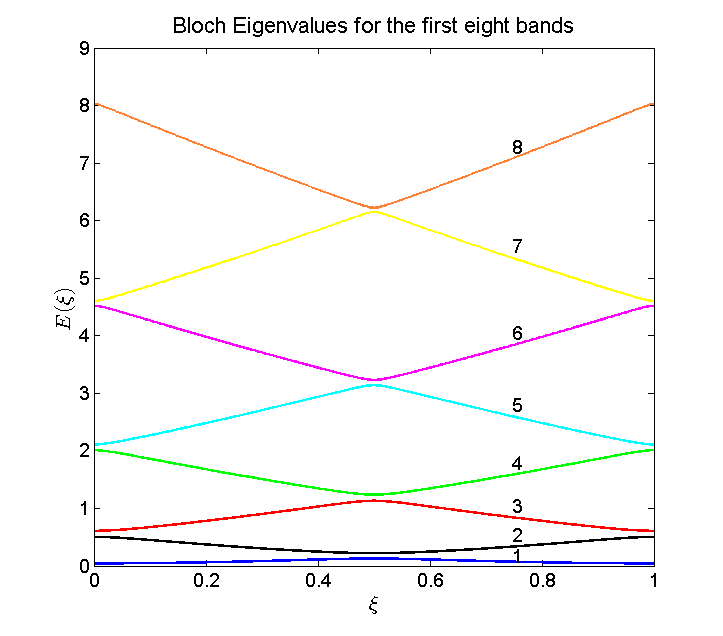
Figure 1. Energy eigenvalues for the one-dimensional lattice potential $V(x)=\exp\left(-25x^{2}\right)$

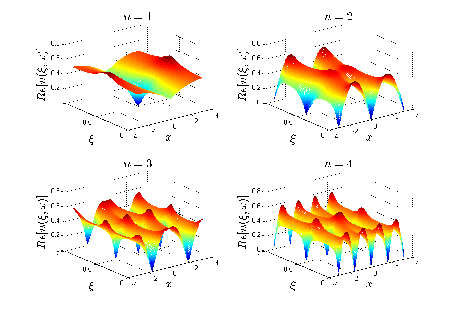
Figure 2. Module of eigenfunctions for the one-dimensional lattice potential $V(x)=\exp\left(-25x^{2}\right)$. We display absolute value of the first 4 lowest energy eigenfunctions.

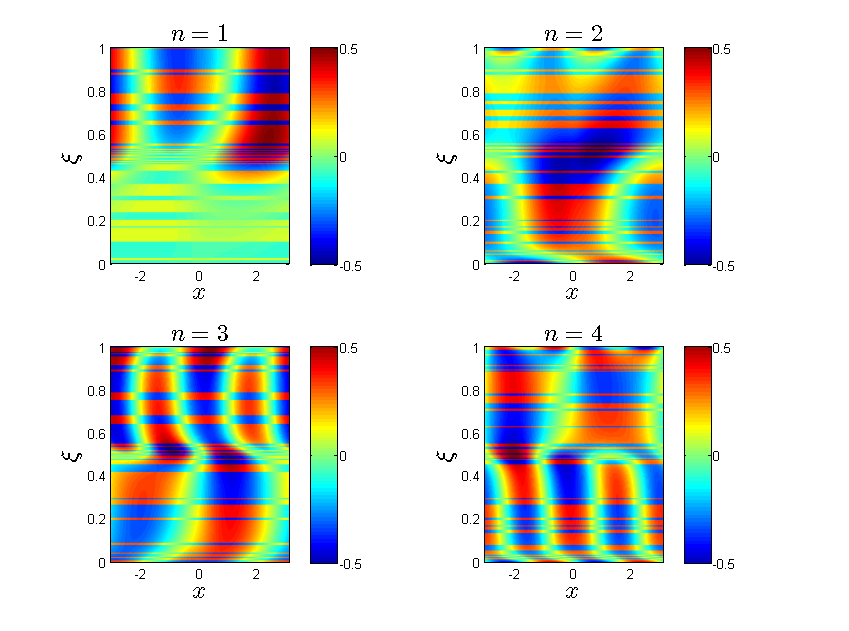
Figure 3. Real part of the eigenfunctions for the one-dimensional lattice potential $V(x)=\exp\left(-25x^{2}\right)$. We display the real parts for the first 4 lowest energy eigenfunctions. We use 100 data points for the $\boldsymbol{\xi}$ variable.

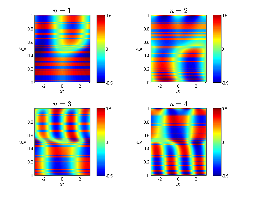
Figure 4. Imaginary part of the eigenfunctions for the one-dimensional lattice potential $V(x)=\exp\left(-25x^{2}\right)$. We display the imaginary parts for the first 4 lowest energy eigenfunctions. We use 100 data points for the $\boldsymbol{\xi}$ variable.

Remark.

1. In the numerical computation of $E(\xi)$, the corresponding eigenfunctions and their derivatives near the points $\xi=0$ and $\xi=0.5$ (and $\xi=1$ by periodicity) is tricky, since the Bloch bands are close to each other near these points (see Figure 1). For this reason, our grid for the $\xi$ variable will not contain these points. In other words, we shift the grids in the first Brillouin zone to avoid these high symmetry points.

2. One can apply the same technique to derive an algorithm for computing Bloch eigenvalues and eigenfunctions in higher dimensions. The main issue with this algorithm is that the numerical cost increases drastically for $d>1$. In the case where the periodic potential has the form $V_{\Gamma}(\boldsymbol{x})=\sum_{j=1}^{d}V_{j}(x_{j})$ with $V_{j}(x_{j}+2\pi)=V(x_{j})$, computation of Bloch bands can be treated for each coordinate $x_{j}$ separately. For some common potentials, data for the energy eigenvalues has already been produced (see remark 2.1 in [HuJiMaSp:07]).

3.2. Algorithms for gauge invariant frozen Gaussian approximation

We assume that the initial data $\psi_{0}(x)$ has compact support or that it decays sufficiently fast as $\lvert x\rvert\rightarrow\infty$, and hence, we only need to use a finite number of mesh points in physical space.

For a mesh size $\delta x$ and starting point $x^{0}\in\mathbb{R}$, the grid is specified as

(3.6) $$x^{m}=x^{0}+(m-1)\delta x,$$

for $m=1,\cdots,N_{x}$, where $N_{x}$ is the number of the spatial grid in one dimension.

We present the algorithm in five steps below.

Step 1. Compute the Bloch eigenvalues $E_{n}(\xi)$ and eigenfunctions $u_{n}(\xi,x)$ of (1.3), according to the algorithm described in Section 3.1.