Scalar field correlator in de Sitter space at next-to-leading
order in a $1/N$ expansion

Abstract

We study the dynamics of light quantum scalar fields in de Sitter space on superhorizon scales. We compute the self-energy of an $O(N)$ symmetric theory at next-to-leading order in a $1/N$ expansion in the regime of superhorizon momenta, and we obtain an exact analytical solution of the corresponding Dyson-Schwinger equations for the two-point correlator. This amounts to resumming the infinite series of nonlocal self-energy insertions, which typically generate spurious infrared and/or secular divergences. The potentially large de Sitter logarithms resum into well-behaved power laws from which we extract the field strength and mass renormalization. The nonperturbative $1/N$ expansion allows us to discuss the case of vanishing and negative tree-level square mass, which both correspond to strongly coupled effective theories in the infrared.

I Introduction

Understanding the dynamics of quantum fields in curved spacetime is a topic of general interest with important applications to early Universe cosmology or black hole physics. Prominent examples are the primordial density fluctuations during inflation Mukhanov:1990me and the Hawking/Unruh radiation from (analog) black holes Hawking:1974sw ; Unruh:1976db ; Brout:1995rd . The case of de Sitter space has attracted particular attention both because of its relevance for inflationary cosmology and because it provides a simple, maximally symmetric example where the nontrivial aspects of the curved geometry come into play.

The investigation of quantum field dynamics on de Sitter space has many facets. A general class of studies concerns the solutions of the field equations of motion in a fully de Sitter symmetric state. Renormalizability and the equivalence principle select the so-called Chernikov-Tagirov-Bunch-Davies (CTBD) state Chernikov:1968zm ; Bunch:1978yq out of the class of Allen-Mottola $\alpha$-vacua Allen:1985ux ; Mottola:1984ar ; Anderson:2005hi . Topical questions include the calculation of radiative corrections to the field dynamics Shore:1979as ; Buchbinder1992 ; Elizalde:1993ee ; Prokopec:2002jn ; Onemli:2002hr ; Brunier:2004sb ; Weinberg:2005qc ; Tsamis:2005hd ; Boyanovsky:2005px ; Sloth:2006az ; Seery:2007we ; vanderMeulen:2007ah ; Serreau:2011fu ; Prokopec:2011ms ; Arai:2011dd ; Serreau:2013koa ; Nacir:2013xca ; Herranen:2013raa ; Onemli:2013gya , the relevance of global coordinate systems as compared to the (expanding) Poincaré patch, of interest for inflationary cosmology Krotov:2010ma ; Akhmedov:2012dn ; Anderson:2013ila , and the relation between Lorentzian and Euclidean de Sitter spaces Rajaraman:2010xd ; Beneke:2012kn ; Marolf:2010nz ; Hollands:2010pr ; Higuchi:2010xt ; Hollands:2014eia . Other studies concern other (possibly non de Sitter invariant) states, e.g., in the context of inflationary cosmology Danielsson:2002kx ; Anderson:2005hi ; Onemli:2002hr , or in relation with the question of the quantum stability of de Sitter space Mottola:1984ar ; Mottola:1985qt ; Tsamis:1996qq ; Polyakov:2009nq ; Krotov:2010ma ; Marolf:2010nz ; Anderson:2013ila ; Akhmedov:2013vka .

An important issue is the understanding of interacting field theories. Not only are these more difficult to tackle than in flat space for obvious technical reasons, but the nontrivial gravitational field leads to specific effects with no flat space analog. Striking examples are the possibility of curvature-induced phase transitions Shore:1979as ; Buchbinder1992 ; Elizalde:1993ee , the decay of massive particles into themselves Bros:2006gs ; Jatkar:2011ju , the generation of a nonvanishing photon mass Prokopec:2002jn ; Prokopec:2003tm ; Prokopec:2007ak , and the radiative restoration of spontaneously broken symmetries Ratra:1984yq ; Mazzitelli:1988ib ; Serreau:2011fu ; Lazzari:2013boa ; Serreau:2013eoa ; Guilleux:2015pma . In the CTBD vacuum, light scalar fields in units of the spacetime curvature exhibit large, gravitationally enhanced quantum fluctuations on superhorizon scales. Notably, this is at the origin of the scale invariance of the (tree-level) power spectrum of primordial density fluctuations in inflationary cosmology. However, such large fluctuations are also responsible for the strong infrared sensitivity of radiative corrections. Perturbation theory typically exhibits infrared and secular (large time) divergences Brunier:2004sb ; Weinberg:2005qc ; Tsamis:2005hd ; Onemli:2013gya . The former are generic for massless bosonic field theories Blaizot:2003tw while the latter are characteristic of nonequilibrium systems Berges:2004vw . Both types of (spurious) divergences signal a breakdown of the perturbative expansion and need to be resummed.

Various resummation methods or genuine nonperturbative approaches have been devised to deal with such issues in de Sitter space. The most prominent one is the stochastic effective theory put forward in Refs. Starobinsky:1986fx ; Starobinsky:1994bd . This has been shown to correctly capture the nonperturbative dynamics of superhorizon modes at leading order accuracy both in secular logarithms Tsamis:2005hd ; Miao:2006pn ; Prokopec:2007ak and in infrared enhancement factors Garbrecht:2013coa ; Garbrecht:2014dca . More recent approaches employ various quantum field theoretical tools such as large-$N$ techniques Mazzitelli:1988ib ; Riotto:2008mv ; Serreau:2011fu ; Serreau:2013psa ; Serreau:2013koa , renormalization group methods Burgess:2009bs ; Kaya:2013bga ; Serreau:2013eoa ; Guilleux:2015pma , the Wigner-Weisskopf approach Boyanovsky:2011xn ; Boyanovsky:2012qs , reduced density matrices Boyanovsky:2015tba , and solutions of the Kadanoff-Baym equations (KBEs) KB ; Berges:2004yj —the nonequilibrium version of the Dyson-Schwinger equations—and their Boltzmann limit Kitamoto:2010si ; Jatkar:2011ju ; Garbrecht:2011gu ; Akhmedov:2011pj ; Akhmedov:2012pa ; Akhmedov:2013xka ; Akhmedov:2013vka ; Youssef:2013by ; Serreau:2013psa ; Gautier:2013aoa ; Rajaraman:2015dta .

In Ref. Gautier:2013aoa , we have studied the KBEs for the correlator of an $O(N)$ scalar field theory with quartic self-interactions using the physical momentum representation of de Sitter correlators Parentani:2012tx ; Busch:2012ne ; Adamek:2013vw . We have obtained an exact analytical solution for the two-point correlator in the regime of superhorizon momenta when the self-energy is computed at two-loop order in perturbation theory. The secular divergences of perturbative calculations of the correlator Brunier:2004sb ; Weinberg:2005qc ; Tsamis:2005hd ; Onemli:2013gya are a mere artifact of expanding the latter in terms of self-energy insertions at a finite order. Solving the KBEs amounts to resumming the infinite series of such self-energy insertions—and thus the associated large infrared logarithms—which results in a modified power law behavior of the correlator. This is similar to the generation of an anomalous dimension for critical systems in statistical physics. From the (resumed) propagator, we could compute various quantities of interest, such as the infrared field strength and mass renormalization, at two-loop order. The applicability of such perturbative computations is limited to not too light fields. The cases of fields with either vanishing or negative tree-level square mass suffer from infrared divergences and require further resummations.

In the present article, we generalize this approach to the nonperturbative $1/N$ expansion at next-to-leading order (NLO). The leading-order (LO) approximation resums the infrared divergences of perturbation theory into a self-consistent (local) mass term. This captures interesting nontrivial physics, such as dynamical mass generation and radiative symmetry restoration Mazzitelli:1988ib ; Serreau:2011fu , or nonperturbative quantum contributions to non-Gaussian correlators Serreau:2013psa ; Serreau:2013koa . The NLO approximation involves an infinite series of nonlocal multiloop contributions to the self-energy. For infrared momenta, the latter can be summed in a closed form using the results of Ref. Serreau:2013psa . The NLO self-energy has a similar form as the two-loop expression, however, with different infrared power law exponents. This allows us to obtain an exact analytical solution of the corresponding KBEs in the infrared regime using the techniques developed in our previous work Gautier:2013aoa .

We thus obtain the complete spacetime structure of the propagator for superhorizon momenta at NLO in the $1/N$ expansion. As in the two-loop case, the infrared logarithms of perturbation theory resum into a superposition of well-behaved momentum power laws, which characterize the decay of the field correlator at large spacetime separations. We compute the leading infrared behavior for deep superhorizon momenta, from which we extract the field strength and mass renormalization. These receive NLO corrections which are nonperturbative functions of the field self-coupling. We study the cases of vanishing and negative tree-level square mass, which both correspond to effectively strongly coupled regimes in the infrared. Finally, we compute the local field variance, which agrees with the result of the stochastic approach at the same approximation order.

The paper is organized as follows. Section II describes the setup and briefly reviews the formulation of KBEs in the $p$-representation Parentani:2012tx . We compute the self-energy at NLO in the $1/N$ expansion in Sec. III and present the solution of the corresponding KBEs in Sec. IV. The NLO result requires the solution of an appropriate gap equation for the local mass, which is described in Sec. V. We discuss our analytical solution for the field correlator in various regimes of interest in Sec. VI, and we conclude in Sec. VII. Finally, some technical details and calculations are presented in Appendixes A–C.

II General setting: KBEs in the $p$-representation

We consider an $O(N)$ scalar field theory on the expanding Poincaré patch of de Sitter space in $D=d+1$ dimensions. In conformal time $-\infty<\eta<0$ and comoving spatial coordinates $\mathbb{X}$, the invariant line element reads (we set the Hubble scale $H=1$)

$$ds^{2}=\eta^{-2}(-d\eta^{2}+d\mathbb{X}.d\mathbb{X}).$$ (1)

The classical action is given by

$$\mathcal{S}=\int_{x}\left\{\frac{1}{2}\varphi_{a}\left(\square-m_{\rm dS}^{2}\right)\varphi_{a}-\frac{\lambda}{4!N}(\varphi_{a}\varphi_{a})^{2}\right\},$$ (2)

with $\int_{x}=\int d^{D}x\sqrt{-g(x)}$ the invariant measure—$g(x)$ is the determinant of the metric—and where summation over repeated indices $a=1,\ldots,N$ is understood. Here, $\square$ is the appropriate Laplace-Beltrami operator and $m_{\mathrm{dS}}^{2}=m^{2}+\xi\mathcal{R}$ includes a possible coupling to the Ricci scalar $\mathcal{R}=d(d+1)$. We consider a symmetric state such that $\langle\varphi_{a}\rangle=0$ and the correlator $G$ and the self-energy $\Sigma$ are diagonal, e.g., $G_{ab}=\delta_{ab}G$. In the rest of the paper we assume a de Sitter invariant state given by the free field CTBD vacuum in the remote past $\eta\to-\infty$.

The covariant inverse propagator is given by

$$G^{-1}(x,x^{\prime})=G^{-1}_{0}(x,x^{\prime})-\Sigma(x,x^{\prime}),$$ (3)

where

$$iG_{0}^{-1}(x,x^{\prime})=\left(\Box_{x}-m_{\mathrm{dS}}^{2}\right)\delta^{(D)}(x,x^{\prime}),$$ (4)

with $\delta^{(D)}(x,x^{\prime})=\delta^{(D)}{(x-x^{\prime})}/\sqrt{-g(x)}$. Extracting a possible local part from the self-energy, one writes

$$\Sigma(x,x^{\prime})=-i\sigma\delta^{(D)}(x,x^{\prime})+\bar{\Sigma}(x,x^{\prime}),$$ (5)

where the local $\sigma$ part is constant for a de Sitter invariant state. We include it in a redefinition of the mass

$$M^{2}=m^{2}_{\mathrm{dS}}+\sigma$$ (6)

and define, accordingly, the propagator

$$iG_{M}^{-1}(x,x^{\prime})=\left(\Box_{x}-M^{2}\right)\delta^{(D)}(x,x^{\prime}),$$ (7)

in terms of which we have

$$G^{-1}(x,x^{\prime})=G^{-1}_{M}(x,x^{\prime})-\bar{\Sigma}(x,x^{\prime}).$$ (8)

The aim of the present work is to solve this equation for $G$ when the self-energy (5) is computed at NLO in a $1/N$ expansion. The main difficulty concerns the convolution with the nonlocal kernel $\bar{\Sigma}(x,x^{\prime})$ when inverting Eq. (8). To this aim, we shall exploit the techniques developed in Refs. Parentani:2012tx ; Serreau:2013psa ; Gautier:2013aoa , which rely on exploiting the de Sitter symmetries in a physical momentum representation, the so-called $p$-representation.

Exploiting the spatial homogeneity and isotropy in comoving coordinates, one writes

$$G(x,x^{\prime})=\int\frac{d^{d}K}{(2\pi)^{d}}\,\,e^{i\mathbb{K}\cdot({\bf X}-{\bf X}^{\prime})}\tilde{G}(\eta,\eta^{\prime},K).$$ (9)

De Sitter symmetries guarantee that the correlator admit the following scaling form Parentani:2012tx

$$\tilde{G}(\eta,\eta^{\prime},K)=\frac{(\eta\eta^{\prime})^{\frac{d-1}{2}}}{K}\hat{G}(p,p^{\prime}),$$ (10)

where $p=-K\eta$ and $p^{\prime}=-K\eta^{\prime}$ are the physical momenta associated with the comoving momentum $K$ at times $\eta$ and $\eta^{\prime}$ respectively. Similarly, the $p$-representation of the self-energy is

$$\tilde{\Sigma}(\eta,\eta^{\prime},K)=(\eta\eta^{\prime})^{\frac{d+3}{2}}K^{3}\hat{\Sigma}(p,p^{\prime}).$$ (11)

Solving the Schwinger-Dyson equation (8) for the propagator $G$ for a given self-energy $\bar{\Sigma}$ in de Sitter space can be viewed as an initial value problem with initial data to be specified in the infinite past $\eta\to-\infty$. This can be formulated by introducing a closed contour in time—the so-called in-in or Schwinger-Keldysh formalism Berges:2004yj —which allows one to conveniently grab together the various components of Green’s functions. Exploiting the way time and momentum are tight together by gravitational redshift in de Sitter spacetime, the time evolution can be traded for a momentum evolution, with initial data to be specified at $p\to+\infty$. Introducing a closed contour $\hat{\mathcal{C}}$ in momentum, the propagator reads Parentani:2012tx

$$\hat{G}(p,p^{\prime})=\hat{F}(p,p^{\prime})-\frac{i}{2}{\rm sign}_{\hat{\mathcal{C}}}(p-p^{\prime})\,\hat{\rho}(p,p^{\prime})$$ (12)

where $\hat{F}$ and $\hat{\rho}$ denote the $p$-representations of the statistical and spectral two-point functions respectively. Here, the sign function is to be understood along the contour $\hat{\mathcal{C}}$; see Ref. Parentani:2012tx for details. Notice the symmetry properties $\hat{F}(p,p^{\prime})=\hat{F}(p^{\prime},p)$, and $\hat{\rho}(p,p^{\prime})=-\hat{\rho}(p^{\prime},p)$. The (nonlocal) self-energy $\hat{\Sigma}(p,p^{\prime})$ admits a similar decomposition.

The Dyson-Schwinger equations expressed in the in-in formalism are called the Kadanoff-Baym equations KB ; Berges:2004yj . In the $p$-representation, they read Parentani:2012tx

$$\left[\partial_{p}^{2}+1-\frac{\nu^{2}-\frac{1}{4}}{p^{2}}\right]\!\hat{F}(p,p^{\prime}) +\int_{p}^{\infty}\!\!\!ds\,\hat{\Sigma}_{\rho}(p,s)\hat{F}(s,p^{\prime})$$

$$=\int_{p^{\prime}}^{\infty}\!\!\!ds\,\hat{\Sigma}_{F}(p,s)\hat{\rho}(s,p^{\prime})$$ (13)

and

$$\left[\partial_{p}^{2}+1-\frac{\nu^{2}-\frac{1}{4}}{p^{2}}\right]\hat{\rho}(p,p^{\prime})=\int^{p}_{p^{\prime}}\!ds\,\hat{\Sigma}_{\rho}(p,s)\hat{\rho}(s,p^{\prime}),$$ (14)

where we introduced (the last equality defines $\varepsilon$)

$$\nu=\sqrt{\frac{d^{2}}{4}-M^{2}}\equiv\frac{d}{2}-\varepsilon.$$ (15)

In the following, we consider light fields in units of the spacetime curvature, i.e., $\varepsilon\approx M^{2}/d\ll 1$.

As announced, momentum here plays the role of the time-evolution variable. It is remarkable that the KBEs effectively reduce to a $(0+1)$-dimensional dynamical problem in the $p$-representation. In fact, the space dimensionality is completely hidden in the expression of the self-energy through $d$-dimensional loop integrals. The statistical function $\hat{F}$ encodes the information about the actual quantum state of the system. Having in mind an adiabatic switch-on of the interactions, the initial data corresponding to the CTBD vacuum are given by $\hat{F}(p,p^{\prime})|_{p=p^{\prime}\to+\infty}=1/2$, $\partial_{p}\hat{F}(p,p^{\prime})|_{p=p^{\prime}\to+\infty}=0$, $\partial_{p}\partial_{p^{\prime}}\hat{F}(p,p^{\prime})|_{p=p^{\prime}\to+\infty}=1/2$. The nontrivial initial data for the spectral function is determined by the equal-time commutation relations: $\partial_{p}\hat{\rho}(p,p^{\prime})|_{p=p^{\prime}}=-1$.

III The self-energy at NLO

We now come to the calculation of the self-energy at NLO in a $1/N$ expansion. This has been discussed in the context of nonequilibrium QFT in Minkowski spacetime in Refs. Berges:2001fi ; Aarts:2002dj . In de Sitter spacetime the corresponding expressions have been derived in the $p$-representation in Ref. Parentani:2012tx . Here, we briefly review the material relevant for our present purposes.

The local contribution in Eq. (5) can be written in closed form in terms of the exact propagator as

$$\sigma=\frac{\lambda}{6}\left(1+\frac{2}{N}\right)\int_{\bf q}\frac{\hat{F}(q,q)}{q},$$ (16)

where $\int_{\bf q}=\int d^{d}q/(2\pi)^{d}$. This is represented diagrammatically in Fig. 1. The corresponding expression at NLO is obtained by plugging the (yet unknown) NLO correlator on the right-hand side and discarding terms of ${\cal O}(1/N^{2})$. As we shall see below, this actually provides a self-consistent equation for the so-called tadpole mass $M$ defined in Eq. (6). For now, we do not need the expression of $M$ and leave it as a free parameter in the calculation.

Figure 1: The local contribution to the self-energy $\Sigma(x,x^{\prime})$; see Eq. (5). The internal line in the diagram is given by the full propagator $G(x,x)$.

Figure 2: A typical multiloop diagram contributing to the nonlocal self-energy $\bar{\Sigma}(x,x^{\prime})$ at NLO. The latter actually resums all diagrams of similar topology with an arbitrary number $n\geq 1$ of bubbles in the upper part, as described by the integral equation (18) in the $p$-representation.

The nonlocal part of the self-energy reads, at NLO,

$$\hat{\Sigma}(p,p^{\prime})=\frac{\lambda}{3N}\,(pp^{\prime})^{d-3\over 2}\!\!\int_{\bf q}\,\frac{r}{q}\,\hat{G}_{M}\left(qp,qp^{\prime}\right)\hat{I}\left(rp,rp^{\prime}\right)\,$$ (17)

where $r=|{\bf e}+{\bf q}|$, with ${\bf e}$ an arbitrary unit vector, and where the function $\hat{I}$ resums the infinite series of bubble diagrams represented in Fig. 2. It solves the following integral equation:

$$\hat{I}(p,p^{\prime})=\hat{\Pi}(p,p^{\prime})-i\int_{\hat{\mathcal{C}}}ds\,\hat{\Pi}(p,s)\hat{I}(s,p^{\prime}),$$ (18)

where the momentum convolution on the right-hand side is to be taken on the momentum contour $\hat{\mathcal{C}}$ to account for the in-in formulation of the problem and where $\hat{\Pi}$ is the one-loop bubble integral

$$\hat{\Pi}(p,p^{\prime})=-\frac{\lambda}{6}\,(pp^{\prime})^{d-3\over 2}\!\!\int_{\bf q}\frac{\hat{G}_{M}\left(qp,qp^{\prime}\right)}{q}\frac{\hat{G}_{M}\left(rp,rp^{\prime}\right)}{r},$$ (19)

with $r=|{\bf e}+{\bf q}|$. Notice that we have used the propagator $G_{M}$ in the NLO expressions (17)–(19). This is consistent because the LO propagator is given by $G_{M_{0}}$ with $M_{0}$ the LO tadpole mass. Here, we shall keep $G_{M}$ in the intermediate steps of the calculation for notational simplicity and consistently expand the final expressions in $1/N$.

Let us finally mention that $\hat{\Pi}$, $\hat{I}$, and $\hat{\Sigma}$ all have similar decompositions as in Eq. (12) on the momentum contour $\hat{\mathcal{C}}$. The product $\hat{G}_{M}\hat{G}_{M}$ in the expression (19) of the function $\hat{\Pi}$ gives rise to the combinations $\hat{F}_{\!M}\hat{F}_{\!M}-{1\over 4}\hat{\rho}_{M}\hat{\rho}_{M}$ for $\Pi_{F}$ and $2\hat{F}_{\!M}\hat{\rho}_{M}$ for $\Pi_{\rho}$. Similarly, the product $\hat{G}_{M}\hat{I}$ in (17) yields $\hat{F}_{\!M}\hat{I}_{F}-{1\over 4}\hat{\rho}_{M}\hat{I}_{\rho}$ for $\hat{\Sigma}_{F}$ and $\hat{F}_{\!M}\hat{I}_{\rho}+\hat{\rho}_{M}\hat{I}_{F}$ for $\hat{\Sigma}_{\rho}$. The explicit integral equations satisfied by the components $\hat{I}_{F}$ and $\hat{I}_{\rho}$, obtained from Eq. (18), read

$$\hat{I}_{\rho}(p,p^{\prime})=\hat{\Pi}_{\rho}(p,p^{\prime})+\int^{p^{\prime}}_{p}ds\,\hat{\Pi}_{\rho}(p,s)\hat{I}_{\rho}(s,p^{\prime})$$ (20)

and

$$\hat{I}_{F}(p,p^{\prime}) =\hat{\Pi}_{F}(p,p^{\prime})-\!\int_{p^{\prime}}^{\infty}\!\!ds\,\hat{\Pi}_{F}(p,s)\hat{I}_{\rho}(s,p^{\prime})$$

$$+\!\int_{p}^{\infty}\!\!ds\,\hat{\Pi}_{\rho}(p,s)\hat{I}_{F}(s,p^{\prime}).$$ (21)

Let us recall the approximation strategy used in Refs. Serreau:2013psa ; Gautier:2013aoa for the calculation of correlators for superhorizon momenta $p,p^{\prime}\lesssim 1$. For light fields in units of the spacetime curvature, the relevant dynamics is dominated by the gravitationally amplified superhorizon fluctuations, and we shall neglect the effect of interactions for subhorizon modes. We thus consider a free evolution up to a given scale $\mu\lesssim 1$ below which we fully take into account the field self-interaction. In practice, this amounts to restricting the convolution integrals in Eqs. (13) and (III) to $\int_{p}^{\infty}\to\int_{p}^{\mu}$ and $\int_{p^{\prime}}^{\infty}\to\int_{p^{\prime}}^{\mu}$. We obtain a closed set of integro-differential equations which only involve two-point functions for superhorizon momenta. One can show, using the method developed in Ref. Serreau:2013psa , that the dominant contribution to the loop integrals in Eqs. (17) and (19) for $p,p^{\prime}\lesssim\mu$ comes from loop momenta $qp,qp^{\prime},rp,rp^{\prime}\lesssim\mu$. These integrals can thus be evaluated by using the leading infrared behavior of the propagator, that is,

$$\hat{F}^{\rm IR}_{\!M}(p,p^{\prime}) =\sqrt{pp^{\prime}}\,\frac{F_{\nu}}{(pp^{\prime})^{\nu}},$$ (22)

$$\hat{\rho}^{\rm IR}_{M}(p,p^{\prime}) =-\sqrt{pp^{\prime}}\,{\cal P}_{\nu}\left(\ln\frac{p}{p^{\prime}}\right),$$ (23)

where $F_{\nu}=\left[2^{\nu}\Gamma(\nu)\right]^{2}/{4\pi}$ and ${\cal P}_{\nu}(u)=\sinh(\nu u)/\nu$. The one-loop bubble integral (19) has been computed in Serreau:2013psa and the solution of the integral equation Eq. (18) for infrared momenta has been obtained in closed form. The dominant infrared behaviors of the statistical and spectral components of the infinite series of bubbles $\hat{I}$ read

$$\hat{I}_{F}^{\rm IR}(p,p^{\prime}) =-\frac{\pi_{\rho}}{\sqrt{pp^{\prime}}}\frac{F_{\nu}}{(pp^{\prime})^{\bar{\nu}-\varepsilon}},$$ (24)

$$\hat{I}_{\rho}^{\rm IR}(p,p^{\prime}) =\frac{\pi_{\rho}}{\sqrt{pp^{\prime}}}\,{\cal P}_{\bar{\nu}}^{\varepsilon}\left(\ln\frac{p}{p^{\prime}}\right),$$ (25)

where $\varepsilon$ has been defined in Eq. (15),

$$\pi_{\rho}=\frac{\lambda F_{\nu}}{6\varepsilon}\frac{\Omega_{d}}{(2\pi)^{d}}\approx\frac{\lambda}{3M^{2}\Omega_{D+1}},$$ (26)

with $\Omega_{d}=2\pi^{d/2}/\Gamma(d/2)$, $\bar{\nu}=\sqrt{\nu^{2}-\pi_{\rho}}$, and where we defined ${\cal P}_{a}^{b}(u)={\cal P}_{a}(u)e^{-b|u|}$. Equations (24) and (25) are valid provided $\pi_{\rho}\ll 1$. More general expressions can be found in Serreau:2013psa . Writing $\bar{\nu}=d/2-\bar{\varepsilon}$, we thus have $\bar{\varepsilon}\approx\varepsilon+\pi_{\rho}/d\ll 1$.

As discussed in Ref. Serreau:2013psa , the function $\hat{I}$ is of the very same form as the one-loop bubble $\hat{\Pi}$ with the replacement $\nu\to\bar{\nu}$. Formally expanding Eqs. (24) and (25) in $\pi_{\rho}$ generates the infinite series of bubble diagrams, each of which brings an additional power of infrared (secular) logarithms $\pi_{\rho}\ln(pp^{\prime})$ and $\pi_{\rho}\ln(p/p^{\prime})$. The infinite series of such infrared logarithms resum into the modified power laws (24) and (25).

Using the expressions (22)–(25), we can evaluate the dominant infrared behavior of the loop integrals in (17). This is detailed in Appendix A. We obtain

$$\hat{\Sigma}_{F}^{\rm IR}(p,p^{\prime}) =-\frac{\sigma_{\rho}}{(pp^{\prime})^{3/2}}\frac{F_{\nu}}{(pp^{\prime})^{\nu-2\gamma}},$$ (27)

$$\hat{\Sigma}_{\rho}^{\rm IR}(p,p^{\prime}) =\frac{\sigma_{\rho}}{(pp^{\prime})^{3/2}}\,{\cal P}_{\nu}^{2\gamma}\left(\ln\frac{p}{p^{\prime}}\right),$$ (28)

where we defined $\gamma=(\varepsilon+\bar{\varepsilon})/2$ and

$$\sigma_{\rho}=\frac{\pi_{\rho}^{2}}{N}\,\left(1+\frac{\varepsilon}{2\gamma}\right).$$ (29)

We emphasize that, if it is justified to neglect relative corrections of order $\varepsilon$, $\bar{\varepsilon}$, and $\gamma$ in numerical prefactors, one should not do so in the exponents of the various power law dependences in the momenta. Indeed, such corrections become relevant at large values of $|\ln(p/p^{\prime})|$ involved in convolution integrals, as discussed in Refs. Serreau:2013psa ; Gautier:2013aoa ; see also Garbrecht:2013coa ; Garbrecht:2014dca .

IV Solution of the KBEs in the infrared

It is remarkable that the NLO self-energy, Eqs. (27) and (28), has the very same form as the two-loop one obtained in Gautier:2013aoa up to the expression of $\sigma_{\rho}$ and with the replacement $\varepsilon\to\gamma$. This is rooted in the fact that the two-loop self-energy can be written as $\Sigma^{\rm 2-loop}\propto G_{M}^{3}\propto\Pi G_{M}$, with $\Pi$ the one-loop bubble defined in Eq. (19). Now, the NLO self-energy assumes a similar form with the one-loop bubble replaced by the infinite series of bubble diagrams, that is, $\Pi\to I$; see Eq. (17). As mentioned above this simply amounts to a modified exponent $\nu\to\bar{\nu}$. The calculation of the loop integral in Eq. (17) is then essentially the same as in the two-loop case; see Appendix A.

This observation actually allows us to directly use the results of our previous work Gautier:2013aoa for the solution of the KBEs (13) and (14). There, we had shown that, for superhorizon momenta $p,p^{\prime}\lesssim\mu$, these reduce to a single integro-differential equation for a function of one variable, which can be solved exactly by analytical means. Here, we simply quote the relevant results and refer the reader to Ref. Gautier:2013aoa for details.

The statistical and spectral components of the correlator read, for $p,p^{\prime}\lesssim\mu$,

$${\hat{F}^{\rm IR}(p,p^{\prime})}={\sqrt{pp^{\prime}}F_{\nu}}\left\{\frac{c_{+}}{(pp^{\prime})^{\bar{\nu}_{+}-\gamma}}+\frac{c_{-}}{(pp^{\prime})^{\bar{\nu}_{-}-\gamma}}\right\},$$ (30)

and

$$\hat{\rho}^{\rm IR}(p,p^{\prime})=-\sqrt{pp^{\prime}}\,\rho\left(\ln\frac{p}{p^{\prime}}\right),$$ (31)

with

$$\rho(u) =c_{+}{\cal P}^{\gamma}_{\bar{\nu}_{+}}(u)+c_{-}{\cal P}^{\gamma}_{\bar{\nu}_{-}}(u)$$

$$\approx c_{+}{\cal P}_{\bar{\nu}_{+}-\gamma}(u)+c_{-}{\cal P}_{\bar{\nu}_{-}-\gamma}(u),$$ (32)

where the approximate expression in the second line is valid for $|u|\gtrsim 1$. Here, $c_{+}+c_{-}=1$, with, up to corrections ${\cal O}(N^{-2})$,

$$c_{-}=\frac{\sigma_{\rho}}{16\nu^{2}\gamma^{2}}\approx\frac{\sigma_{\rho}}{4d^{2}\gamma^{2}},$$ (33)

and

$$\bar{\nu}_{\pm}=\nu_{\pm}\pm\frac{\sigma_{\rho}}{8\nu\nu_{\pm}\gamma}\approx\nu_{\pm}\pm\frac{\sigma_{\rho}}{2d^{2}\gamma},$$ (34)

where $\nu_{\pm}=\nu\pm\gamma$, and where we neglected terms ${\cal O}(\varepsilon/N,\gamma/N)$ in the final expressions.

As we already observed in the two-loop approximation Gautier:2013aoa , we find that the NLO propagator (30)–(32) is essentially described by a linear superposition of two free massive field propagators with masses $m_{\pm}$ defined as

$$\bar{\nu}_{\pm}-\gamma=\sqrt{\frac{d^{2}}{4}-m_{\pm}^{2}}\equiv\frac{d}{2}-\varepsilon_{\pm}.$$ (35)

Notice that $m_{+}<m_{-}$. Expanding the above solution in powers of $\sigma_{\rho}$ formally corresponds to the infinite series of nonlocal self-energy insertions and generates arbitrary powers of infrared logarithms $\sigma_{\rho}\ln(pp^{\prime})$ or $\sigma_{\rho}\ln(p/p^{\prime})$. These correspond to the infrared secular logarithms obtained in strict perturbative calculations of the field correlator Brunier:2004sb ; Weinberg:2005qc ; Tsamis:2005hd ; Onemli:2013gya . Again, the summation of these contributions through the KBEs yields well-behaved infrared power laws with modified exponents $\nu\to\bar{\nu}_{\pm}-\gamma$. Going back to spacetime variables, the NLO correlator can be written

$$G(x,x^{\prime})=c_{+}G_{m_{+}}(z)+c_{-}G_{m_{-}}(z),$$ (36)

where $G_{m}(z)$ is the propagator of a free scalar field with mass $m\ll 1$ and $z\equiv z(x,x^{\prime})$ is the de Sitter invariant distance between the points $x$ and $x^{\prime}$; see Appendix B.

The solution (30)–(32) is expressed in terms of the tadpole mass $M$. The latter has to be determined self-consistently from the gap equation (6), with the expression (16).

V Determination of the tadpole mass at NLO

The tadpole diagram (16) involves the correlator in the coincidence limit $G(x,x)=\langle\varphi^{2}(x)\rangle/N$. The latter is dominated by the strongly amplified superhorizon fluctuations and can be evaluated using the expression (30). This yields

$$\frac{\langle\varphi^{2}(x)\rangle}{N} =\int\frac{d^{d}p}{(2\pi)^{d}}\frac{\hat{F}(p,p)}{p}$$

$$\approx\frac{F_{\nu}\Omega_{d}}{(2\pi)^{d}}\left(\frac{c_{+}}{d-2(\bar{\nu}_{+}-\gamma)}+\frac{c_{-}}{d-2(\bar{\nu}_{-}-\gamma)}\right)$$

$$\approx\frac{1}{\Omega_{D+1}M^{2}}\left(1+\frac{1}{N}\frac{\pi_{\rho}^{2}}{2d^{2}\varepsilon\gamma}+{\cal O}\left(N^{-2}\right)\right).$$ (37)

The NLO gap equation (6) thus reads

$$M^{2}=m_{\rm dS}^{2}+\frac{\lambda}{6\Omega_{D+1}M^{2}}\left[1+\frac{2}{N}\left(1+\frac{(\gamma_{0}-\varepsilon_{0})^{2}}{\varepsilon_{0}\gamma_{0}}\right)\right],$$ (38)

where we have used $\pi_{\rho}/(2d)\approx\gamma-\varepsilon$ and where the subscript $0$ indicates that the corresponding quantity is evaluated at LO. Equation (38) is solved as

$$\frac{M^{2}}{M_{0}^{2}}=1+\frac{2}{N}\frac{\lambda_{\rm eff}\left(1+\lambda_{\rm eff}+\lambda_{\rm eff}^{2}\right)}{(1+\lambda_{\rm eff})^{2}},$$ (39)

where

$$M_{0}^{2}=\frac{m_{\rm dS}^{2}}{2}+\sqrt{\frac{\left(m_{\rm dS}^{2}\right)^{2}}{4}+\frac{\lambda}{6\Omega_{D+1}}}$$ (40)

is the LO solution Serreau:2011fu (notice that $M_{0}^{2}>0$) and where we introduced the effective coupling

$$\lambda_{\rm eff}=\frac{\lambda}{6\Omega_{D+1}M_{0}^{4}}.$$ (41)

The relevance of the latter stems from the observation that the effective potential for light scalar fields on superhorizon scales is described by an effective zero-dimensional field theory Serreau:2013eoa ; Guilleux:2015pma . Equation (41) corresponds to the dimensionless effective coupling of such a theory at LO in the $1/N$ expansion.

VI Discussion

Let us now discuss some of the peculiar features of the NLO propagator obtained above. In particular, we consider the regime of deep infrared momenta and the corresponding behavior of the field correlator at large spacetime separations as well as the field variance, given by the correlator in the coincident limit. The latter can be compared to the results from other methods such as the stochastic approach or the Euclidean de Sitter approach. We shall examine the relevant quantities in various regimes of parameters from the case of light but massive fields, where perturbation theory applies, to the cases of either zero or negative tree level square mass, described by an effective strongly coupled regime.

VI.1 Deep infrared momenta and large spacetime separations

The dominant contribution to the regime of deep infrared momenta $p,p^{\prime}\ll\mu$ and/or large momentum (time) separation $|\ln(p/p^{\prime})|\propto|t-t^{\prime}|\gg 1$ [where $t=-\ln(-\eta)$ is the cosmological time] is governed by the term with the lowest mass $m_{+}$ on the right-hand side of either Eq. (30) or (32). In this regime, the NLO propagator reduces to that of a renormalized massive field

$$\hat{F}^{\rm IR}(p,p^{\prime}) \approx\sqrt{pp^{\prime}}\,\frac{Z\,F_{\nu_{\rm IR}}}{(pp^{\prime})^{\nu_{\rm IR}}},$$ (42)

$$\hat{\rho}^{\rm IR}(p,p^{\prime}) \approx-\sqrt{pp^{\prime}}\,Z\,{\cal P}_{\nu_{\rm IR}}\left(\ln\frac{p}{p^{\prime}}\right),$$ (43)

where $Z=c_{+}=1-c_{-}$ and, denoting $m_{+}^{2}=m_{\rm IR}^{2}$,

$$\nu_{\rm IR}=\sqrt{{d^{2}\over 4}-m_{\rm IR}^{2}}.$$ (44)

The field renormalization factor is completely due to the NLO nonlocal self-energy and reads, in terms of the effective coupling (41),

$${Z}=1-\frac{\sigma_{\rho}}{4d^{2}\gamma^{2}}\approx 1-\frac{1}{2N}\frac{\lambda_{\rm eff}^{2}(3+2\lambda_{\rm eff})}{(1+\lambda_{\rm eff})^{3}}.$$ (45)

Similarly, the contribution to the infrared mass due to nonlocal self-energy insertions is

$$\frac{m_{\rm IR}^{2}}{M^{2}}=1-\frac{\sigma_{\rho}}{2d^{2}\varepsilon\gamma}\approx 1-\frac{1}{N}\frac{\lambda_{\rm eff}^{2}(3+2\lambda_{\rm eff})}{(1+\lambda_{\rm eff})^{2}}.$$ (46)

Taking into account the NLO tadpole contribution, we finally obtain

$$\frac{m_{\rm IR}^{2}}{M_{0}^{2}}=1+\frac{1}{N}\frac{\lambda_{\rm eff}\,(2-\lambda_{\rm eff})}{(1+\lambda_{\rm eff})^{2}}.$$ (47)

We see that the factor $Z<1$ controls the amplitude of the deep infrared fluctuations in momentum space, whereas $m_{\rm IR}^{2}$ controls the momentum dependence of the correlator and, in turn, its behavior at large spacetime separation, as described in Appendix B.

VI.2 Field variance

Another quantity of interest is the field correlator in the coincidence limit, which measures the local field variance, $G(x,x)=\langle\varphi^{2}(x)\rangle/N$. The latter can be characterized in terms of an effective mass $m_{\rm dyn}$, defined as Beneke:2012kn ; Garbrecht:2011gu

$$\frac{\langle\varphi^{2}(x)\rangle}{N}\equiv\frac{1}{\Omega_{D+1}m_{\rm dyn}^{2}},$$ (48)

in analogy with the expression for a free massive field. In fact, such a square mass is nothing but the curvature of the effective potential of the dimensionally reduced theory Guilleux:2015pma . We have already evaluated the field variance in Eq. (37). This yields, for the contribution of nonlocal self-energy insertions,

$$\frac{m_{\rm dyn}^{2}}{M^{2}}=1-\frac{2}{N}\frac{\lambda_{\rm eff}^{2}}{1+\lambda_{\rm eff}}.$$ (49)

Including the contribution from the NLO tadpole mass, we get

$$\frac{m_{\rm dyn}^{2}}{M_{0}^{2}}=1+\frac{2}{N}\frac{\lambda_{\rm eff}}{(1+\lambda_{\rm eff})^{2}}.$$ (50)

This expression can be compared to the result of the stochastic approach, where the local field fluctuations can be computed at all orders of perturbation theory with leading infrared logarithmic accuracy Tsamis:2005hd . For light fields, this is equivalently given by the variance of the zero mode on Euclidean de Sitter space Beneke:2012kn . We present the calculation of the field variance at NLO in the $1/N$ expansion in the stochastic and Euclidean de Sitter approaches in Appendix C, which completely agree with Eq. (50).

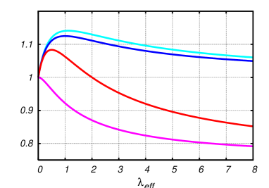
Figure 3: The dimensionless quantities (from bottom to top) $Z$, $m_{\rm IR}^{2}/M_{0}^{2}$, $m_{\rm dyn}^{2}/M_{0}^{2}$, and $m_{\rm IR}^{2}/(ZM_{0}^{2})$ as functions of the dimensionless effective coupling $\lambda_{\rm eff}$ for $N=4$. The two lower curves asymptote to $1-1/N$, whereas the two upper ones asymptote to $1$. Deviations from unity are due to both local and nonlocal $1/N$ corrections.

We emphasize that the result (50) differs from what one would obtain by evaluating the field variance only from the deep IR behavior, Eq. (42). Indeed, this would lead to $\langle\varphi^{2}(x)\rangle/N\to Z/(\Omega_{D+1}m_{\rm IR}^{2})$. The term $\propto c_{-}$ in Eq. (37) is needed to get the correct variance. However, we mention that the ratio $m_{\rm IR}^{2}/Z$ turns out to be numerically close to $m_{\rm dyn}^{2}$ for arbitrary $\lambda_{\rm eff}$. The dimensionless quantities $Z$, $m_{\rm IR}^{2}/M_{0}^{2}$, $m_{\rm IR}^{2}/(ZM_{0}^{2})$, and $m_{\rm dyn}^{2}/M_{0}^{2}$ are plotted against the effective coupling $\lambda_{\rm eff}$ in Fig. 3. Notice the hierarchy $m_{\rm IR}^{2}<m_{\rm dyn}^{2}<m_{\rm IR}^{2}/Z$. It is important to notice that all these square masses are equal to $M_{0}^{2}$ at LO and that their differences are entirely due to the nonlocal self-energy. Since neither the LO nor the NLO tadpole square masses $M_{0}^{2}$ and $M^{2}$ are observable, it is interesting to consider ratios of physical quantities such as

$$\frac{m_{\rm IR}^{2}}{m_{\rm dyn}^{2}} =1-\frac{1}{N}\frac{\lambda_{\rm eff}^{2}}{(1+\lambda_{\rm eff})^{2}},$$ (51)

$$\frac{m_{\rm IR}^{2}}{Zm_{\rm dyn}^{2}} =1+\frac{1}{2N}\frac{\lambda_{\rm eff}^{2}}{(1+\lambda_{\rm eff})^{3}},$$ (52)

whose deviation from unity is entirely an effect of resuming the large infrared logarithms from nonlocal self-energy insertions. The ratios (51) and (52) are plotted against $\lambda_{\rm eff}$ in Fig. 4.

Finally, we note that all the NLO corrections computed in this sections, Eqs. (45), (47), (50), (51), and (52), exhibit a nontrivial dependence in the (effective) coupling and are actually bounded functions of the latter due to nonperturbative $1/N$ corrections. The NLO results thus remain valid for arbitrarily large effective couplings. We shall now discuss the various cases of interest, from the weak coupling, perturbative regime to the strongly coupled one.

VI.3 Perturbative regime

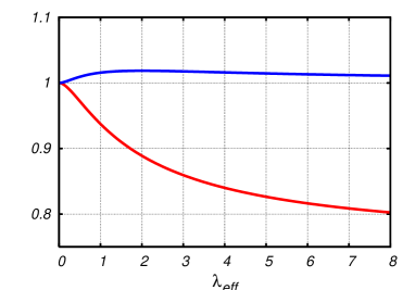
Figure 4: The dimensionless ratios of physical quantities $m_{\rm IR}^{2}/m_{\rm dyn}^{2}$ (lower curve) and $m_{\rm IR}^{2}/(Zm_{\rm dyn}^{2})$ (upper curve) as functions of the dimensionless effective coupling $\lambda_{\rm eff}$ for $N=4$. These asymptote to $1-1/N$ and $1$, respectively at large coupling. Deviations from unity are entirely due to nonlocal $1/N$ corrections.

Perturbation theory makes sense whenever the quadratic part of the action (2) gives the dominant contribution to physical observables. This corresponds to the case of light but massive field, with $\sqrt{\lambda}\ll m_{\rm dS}^{2}\ll 1$ Burgess:2009bs ; Garbrecht:2013coa ; Garbrecht:2014dca . In that case, one has $M_{0}^{2}=m_{\rm dS}^{2}[1+\bar{\lambda}_{0}-\bar{\lambda}_{0}^{2}+{\cal O}(\bar{\lambda}_{0}^{3})]$, $\lambda_{\rm eff}=\bar{\lambda}_{0}[1-2\bar{\lambda}_{0}+{\cal O}(\bar{\lambda}_{0}^{2})]\ll 1$, where we defined

$$\bar{\lambda}_{0}=\frac{\lambda}{6\Omega_{D+1}\left(m_{\rm dS}^{2}\right)^{2}}.$$ (53)

We get

$$Z=1-\frac{3\bar{\lambda}_{0}^{2}}{2N}$$ (54)

and

$$m_{\rm IR}^{2} =m_{\rm dS}^{2}\!\left[1+\!\left(1+\frac{2}{N}\right)\!\bar{\lambda}_{0}-\!\left(1+\frac{7}{N}\right)\!\bar{\lambda}_{0}^{2}+{\cal O}\!\left(\bar{\lambda}_{0}^{3}\right)\right],$$ (55)

$$m_{\rm dyn}^{2} =m_{\rm dS}^{2}\!\left[1+\!\left(1+\frac{2}{N}\right)\!\bar{\lambda}_{0}-\!\left(1+\frac{6}{N}\right)\!\bar{\lambda}_{0}^{2}+{\cal O}\!\left(\bar{\lambda}_{0}^{3}\right)\right]\!.$$ (56)

These expressions agree with the two-loop results of Ref. Gautier:2013aoa at the relevant order in $1/N$, as they should.

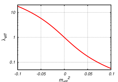
Figure 5: The dimensionless effective coupling (41) as a function of the tree-level square mass $m_{\rm dS}^{2}$ for $\lambda=10^{-1}$ in $D=3+1$ dimensions. Large positive values of $m_{\rm dS}^{2}$ in units of $\sqrt{\lambda/(6\Omega_{D+1})}\approx 0.025$ correspond to perturbatively small effective couplings, whereas small or large negative values correspond to $\lambda_{\rm eff}\approx 1$ and $\lambda_{\rm eff}\gg 1$, respectively.

VI.4 Massless case

More interesting for our present purposes are theories with very small tree-level mass, such that $\bar{\lambda}_{0}\gg 1$, or with negative tree-level mass, $m_{\rm dS}^{2}<0$. Both cases correspond to strongly coupled effective theories in the infrared, as measured by the effective coupling (41); see Fig. 5. We first consider the light mass case. It is well known that, even for massless fields, the scalar self-interactions generate a nonvanishing effective mass. At LO the latter is $M_{0}^{2}=\sqrt{\lambda/(6\Omega_{D+1})}$ and the effective coupling $\lambda_{\rm eff}\approx 1$. We thus get, at NLO,

$$Z=1-\frac{5}{16N}$$ (57)

and

$$m_{\rm IR}^{2} =\sqrt{\frac{\lambda}{6\Omega_{D+1}}}\left(1+\frac{1}{4N}\right),$$ (58)

$$m_{\rm dyn}^{2} =\sqrt{\frac{\lambda}{6\Omega_{D+1}}}\left(1+\frac{1}{2N}\right).$$ (59)

VI.5 Negative square mass case

Finally, in the case of a negative tree-level square mass, the apparently broken symmetry gets radiatively restored by the strong, gravitationally amplified superhorizon fluctuations Ratra:1984yq ; Mazzitelli:1988ib ; Serreau:2011fu . For $\bar{\lambda}_{0}\ll 1$, one has $M_{0}^{2}\approx\lambda/(6\Omega_{D+1}|m_{\rm dS}^{2}|)=\bar{\lambda}_{0}|m_{\rm dS}^{2}|$ and the effective infrared theory is strongly coupled: $\lambda_{\rm eff}\approx 1/\bar{\lambda}_{0}\gg 1$. We obtain

$$Z=1-\frac{1}{N}$$ (60)

and

$$m_{\rm IR}^{2} =\bar{\lambda}_{0}|m_{\rm dS}^{2}|\left(1-\frac{1}{N}\right),$$ (61)

$$m_{\rm dyn}^{2} =\bar{\lambda}_{0}|m_{\rm dS}^{2}|\left(1+\frac{2}{N}\bar{\lambda}_{0}\right).$$ (62)

VII Summary and perspectives

Quantum field theoretical calculations in curved spacetimes are technically involved as compared to their Minkowski counterparts because of the nontrivial symmetries of the background geometry. Even the calculation of the basic two-point correlator of a self-interacting scalar field in the maximally symmetric de Sitter space is a notoriously difficult task due to the nontrivial convolution/memory integrals involving the nonlocal self-energy. For cosmological spacetimes, the problem can be cast in the form of a nonequilibrium, initial value setup Tranberg:2008ae . A strict perturbative expansion in powers of self-energy insertions leads to spurious secular divergences typical of nonequilibrium systems Berges:2004vw . Solving the integro-differential KBEs is formally equivalent to resumming the infinite series of self-energy insertions and yields a well-defined late-time behavior. Together with Refs. Gautier:2013aoa , the present work provides techniques to formulate and solve KBEs in de Sitter spacetime in the case of light fields. Related work for massive fields or for non de Sitter invariant states can be found in Refs Kitamoto:2010si ; Jatkar:2011ju ; Garbrecht:2011gu ; Akhmedov:2011pj ; Akhmedov:2012pa ; Akhmedov:2013xka ; Akhmedov:2013vka ; Youssef:2013by .

In the present article, we have computed the two-point correlator of an $O(N)$ scalar field in the regime of superhorizon momenta at NLO in a $1/N$ expansion. Remarkably the solution can be obtained in closed analytical form. This resums the spurious infrared and secular divergences of perturbation theory into a well-defined expression. The nonperturbative $1/N$ expansion allows us to compute various quantities of interest, such as the infrared field strength and mass renormalization, or the local field variance, for arbitrary values of the field self-coupling. In particular, this is a valid approximation scheme for the cases of either vanishing or negative tree-level square mass, which correspond to effectively strongly coupled regimes not accessible by perturbative means.

The local field variance $\langle\varphi^{2}(x)\rangle$ obtained here fully agrees with the result of either the stochastic, or the Euclidean de Sitter approaches—which are in fact equivalent for what concerns this observable Rajaraman:2010xd ; Beneke:2012kn — as well as the recently proposed nonperturbative renormalization group approach of Refs. Serreau:2013eoa ; Guilleux:2015pma . Our result further gives the full spacetime structure of the correlator for noncoincident points at large spacetime separations. To the best of our knowledge, this has never been computed before. It would be of definite interest to perform such a calculation in, say, the stochastic effective theory for a comparison. More generally, it would be interesting to make a precise link between the present approach and the stochastic theory, e.g., along the lines of Refs. Garbrecht:2013coa ; Garbrecht:2014dca ; Gautier:2012vh .

Interesting extensions of the present work include the generalization of the techniques developed here to other types of (e.g., fermionic or gauge) fields and/or to theories with more complicated (e.g., derivative) interactions. Also of interest is the study of other spacetime geometries, such as quasi-de Sitter space and general cosmological spacetimes, or black hole geometries, of interest for the question of radiative corrections to the Hawking radiation Akhmedov:2015xwa .

Appendix A Self-energy at NLO

Here, we compute the nonlocal contribution (17) to the NLO self-energy. As explained before, the multiloop nature of the NLO approximation can be captured by the function $\hat{I}(p,p^{\prime})$. The latter resums the infinite series of bubble diagrams and eventually takes a similar form as a propagator with modified infrared exponent; see Eqs. (24) and (25) [we refer the reader to Ref. Serreau:2013psa for details concerning the calculation of the functions $\hat{I}_{F}(p,p^{\prime})$ and $\hat{I}_{\rho}(p,p^{\prime})$]. The remaining momentum (loop) integral in Eq. (17) can thus be treated using the methods developed in Ref. Serreau:2013psa . For external momenta $p,p^{\prime}\lesssim\mu$, it is dominated by internal (loop) momenta such that $qp,qp^{\prime}\lesssim\mu$, which imply $rp,rp^{\prime}\lesssim\mu$. We can effectively limit the momentum integration to a sphere of radius $\min(\mu/p,\mu/p^{\prime})$ and use the leading infrared behaviors (22)–(25) of the integrands.

We first evaluate the statistical part of the self-energy $\hat{\Sigma}_{F}$. In this case the integrand is proportional to $\hat{F}_{\!M}^{\rm IR}\hat{I}_{F}^{\rm IR}-\rho_{M}^{\rm IR}\hat{I}_{\rho}^{\rm IR}/4\approx\hat{F}_{\!M}^{\rm IR}\hat{I}_{F}^{\rm IR}$. Here, the neglect of the $\rho$-components is justified by the infrared power laws in Eqs. (22) and (24), which results from the amplification of infrared fluctuations. The $\rho$-components are not amplified. We thus get

$$\hat{\Sigma}_{F}^{IR}(p,p^{\prime})\approx-\frac{\lambda F_{\nu}^{2}\pi_{\rho}}{3N(pp^{\prime})^{3/2+\beta}}\int_{{\bf q}}\frac{1}{q^{2\nu}r^{2(\bar{\nu}-\varepsilon)}},$$ (63)

where $\beta=\nu-2\gamma=\bar{\nu}-2\varepsilon$ and $r=|{\bf e}+{\bf q}|$, with ${\bf e}$ an arbitrary unit vector. The remaining integral is rapidly convergent such that one can safely set the upper bound to infinity. It can then be evaluated, e.g., using the method of Feynman parameters,

$$\int_{\mathbb{q}}\frac{1}{q^{2\nu}r^{2(\bar{\nu}-\varepsilon)}} =\frac{\Omega_{d}}{2(2\pi)^{d}}\frac{\Gamma(\varepsilon)\Gamma(2\gamma)}{\Gamma(\varepsilon+2\gamma)}\frac{\Gamma(\nu+\varepsilon)\Gamma(\bar{\nu}-2\varepsilon)}{\Gamma(\nu)\Gamma(\bar{\nu}-\varepsilon)}$$

$$\approx\frac{\Omega_{d}}{(2\pi)^{d}}\left(\frac{1}{2\varepsilon}+\frac{1}{4\gamma}\right),$$ (64)

where we have neglected relative corrections of ${\cal O}(\varepsilon,\gamma)$ in the last line. We finally get

$$\hat{\Sigma}_{F}^{IR}(p,p^{\prime})=-\frac{\sigma_{\rho}F_{\nu}}{(pp^{\prime})^{3/2+\beta}},$$ (65)

where $\sigma_{\rho}$ is defined in Eq. (29).

The integrand for the spectral component $\hat{\Sigma}_{\rho}$ involves the combination $\hat{F}_{\!M}^{\rm IR}\hat{I}_{\rho}^{\rm IR}+\rho_{M}^{\rm IR}\hat{I}_{F}^{\rm IR}$. For $p<p^{\prime}$, it reads

$$\hat{\Sigma}_{\rho}^{IR}(p,p^{\prime})=\frac{\lambda F_{\nu}\pi_{\rho}}{3N}(pp^{\prime})^{\frac{d-3}{2}}$$

$$\times\int_{|\mathbb{q}|\leq\frac{\mu}{p^{\prime}}}\!\left\{\frac{{\cal P}_{\bar{\nu}}\!\left(\ln\frac{p}{p^{\prime}}\right)}{(pp^{\prime})^{\nu}}\!\left(\frac{p}{p^{\prime}}\right)^{\varepsilon}\!\frac{1}{q^{2\nu}}+\frac{{\cal P}_{\nu}\!\left(\ln\frac{p}{p^{\prime}}\right)}{(pp^{\prime})^{\bar{\nu}-\varepsilon}}\frac{1}{q^{2(\bar{\nu}-\varepsilon)}}\right\}\!.$$ (66)

The remaining integrals are trivially performed,

$$\int_{|\mathbb{q}|<\mu/p^{\prime}}\frac{1}{q^{2\alpha}}=\frac{\Omega_{d}}{(2\pi)^{d}(d-2\alpha)}\left(\frac{\mu}{p^{\prime}}\right)^{d-2\alpha}.$$ (67)

Repeating the same calculation for $p>p^{\prime}$, we finally obtain

$$\hat{\Sigma}_{\rho}^{IR}(p,p^{\prime}) \!=\!\frac{\lambda}{3N}\frac{F_{\nu}\pi_{\rho}}{(pp^{\prime})^{3\over 2}}\frac{\Omega_{d}}{(2\pi)^{d}}\!\!\left\{\!\frac{{\cal P}_{\bar{\nu}}^{2\varepsilon}\!\left(\ln\frac{p}{p^{\prime}}\right)}{2\varepsilon}\!+\!\frac{{\cal P}_{\nu}^{2\gamma}\!\left(\ln\frac{p}{p^{\prime}}\right)}{4\gamma}\!\right\}$$

$$\cong\frac{\sigma_{\rho}}{(pp^{\prime})^{3/2}}{\cal P}_{\nu}^{2\eta}\left(\ln\frac{p}{p^{\prime}}\right),$$ (68)

where we have neglected relative corrections of ${\cal O}(\varepsilon,\gamma)$ in the constant factors and where we have used ${\cal P}_{\nu}^{2\eta}(x)\approx{\cal P}_{\nu-2\eta}(x)={\cal P}_{\bar{\nu}-2\varepsilon}(x)\approx{\cal P}_{\bar{\nu}}^{2\varepsilon}(x)$ for $|x|\gtrsim 1$ in obtaining the last expression.

Equations (65) and (68) are the results quoted in the text, Eqs. (27) and (28).

Appendix B Propagator in spacetime

Here, we consider the spacetime structure of the NLO propagator obtained in the present work, Eqs. (30)–(32). The latter can be written as a linear superposition of two free massive propagators with masses $m_{\pm}\ll 1$. We thus consider first the spacetime structure of the propagator of a free light scalar field in its CTBD vacuum. In general, this can be expressed exactly in terms of a hypergeometric function Chernikov:1968zm ; Bunch:1978yq but the case of a light field yields a much simpler form, both in the coincidence limit and at large spacetime separations, that we now discuss.

The statistical propagator of a scalar field with mass $m\ll 1$ receives contributions $\sim 1/m^{2}$ which are generated by the infrared power law (22). Let us first consider the case of large spacelike separations, with spatial comoving distance $|{\bf X}-{\bf X}^{\prime}|^{2}\gg\eta^{2}+\eta^{\prime 2}$. In that case, the oscillating phase in Eq. (9) effectively cuts off the momentum integral at $K|{\bf X}-{\bf X}^{\prime}|\lesssim 1$, and it is fully justified to use the leading infrared behavior of the correlator for $|K\eta|,|K\eta^{\prime}|\ll 1$, given by Eq. (22). Using Eqs. (9), (10), and (22), we have

$$F_{m}^{\rm IR}(x,x^{\prime}) \approx(\eta\eta^{\prime})^{\varepsilon}F_{\nu}\int\frac{d^{d}K}{(2\pi)^{d}}\frac{e^{i{\bf K}\cdot({\bf X}-{\bf X}^{\prime})}}{K^{2\nu}}$$

$$\approx\frac{1}{\Omega_{D+1}m^{2}}\left(\frac{\eta\eta^{\prime}}{|{\bf X}-{\bf X}^{\prime}|^{2}}\right)^{\varepsilon},$$ (69)

where $\nu=d/2-\varepsilon$, with $\varepsilon\approx m^{2}/d$, and where we used

$$\int\frac{d^{d}K}{(2\pi)^{d}}\frac{e^{i{\bf K}\cdot{\bf X}}}{K^{d-2\varepsilon}} =\frac{1}{(4\pi)^{d/2}}\frac{\Gamma(\varepsilon)}{\Gamma(d/2-\varepsilon)}\left(\frac{2}{|{\bf X}|}\right)^{2\varepsilon}$$ (70)

$$\approx\frac{1}{(4\pi)^{d/2}\Gamma(d/2)}\frac{1}{\varepsilon|{\bf X}|^{2\varepsilon}}.$$ (71)

In the case of large timelike separations $|{\bf X}-{\bf X}^{\prime}|^{2}\ll\eta^{2}+\eta^{\prime 2}$, the phase factor $e^{i{\bf K}\cdot({\bf X}-{\bf X}^{\prime})}\approx 1$ in the relevant integration region and the integral in (9) must effectively be cut off at $K\leq\min\left(\frac{\mu}{|\eta|},\frac{\mu}{|\eta^{\prime}|}\right)$ for the use of the leading infrared form (22)—which yields the $1/m^{2}$ contribution to the correlator in spacetime—to be justified. For large time separation, i.e., $|t-t^{\prime}|=|\ln(\eta/\eta^{\prime})|\gg 1$, we can replace the upper bound by $K^{2}\lesssim\frac{\mu^{2}}{\eta^{2}+\eta^{\prime 2}}$, and we obtain

$$F_{m}^{\rm IR}(x,x^{\prime})\approx\frac{1}{\Omega_{D+1}m^{2}}\left(\frac{\eta\eta^{\prime}}{\eta^{2}+\eta^{\prime 2}}\right)^{\varepsilon}=\frac{1}{\Omega_{D+1}m^{2}}e^{-\varepsilon|t-t^{\prime}|},$$ (72)

where we used

$$\int\frac{d^{d}K}{(2\pi)^{d}}\frac{\theta(\Lambda-K)}{K^{d-2\varepsilon}}=\frac{\Omega_{d}}{(2\pi)^{d}}\frac{\Lambda^{2\varepsilon}}{2\varepsilon}=\frac{1}{(4\pi)^{d/2}\Gamma(d/2)}\frac{\Lambda^{2\varepsilon}}{\varepsilon}.$$ (73)

Of course, the correlator is a function of the de Sitter invariant

$$z =\frac{-\eta^{2}-\eta^{\prime 2}+|{\bf X}-{\bf X}^{\prime}|^{2}}{2\eta\eta^{\prime}}$$ (74)

$$=-\cosh(t-t^{\prime})+\frac{|{\bf X}-{\bf X}^{\prime}|^{2}}{2}e^{t+t^{\prime}}.$$ (75)

The expressions (69) and (72) simply rewrite, up to relative corrections ${\cal O}(\varepsilon)$,

$$F_{m}^{IR}(x,x^{\prime})\approx\frac{1}{\Omega_{D+1}m^{2}|z|^{\varepsilon}}\quad{\rm for}\quad|z|\gg 1$$ (76)

in the relevant limits of large spacelike or timelike separations. The leading $1/m^{2}$ behavior (76) can also be obtained directly from the expression of the exact propagator in terms of hypergeometric functions Garbrecht:2013coa .

Finally, we note that the expression (76) also holds in the coincidence limit $z\to 1$, for which

$$F_{m}^{\rm IR}(x,x)\approx\eta^{2\varepsilon}F_{\nu}\int\frac{d^{d}K}{(2\pi)^{d}}\frac{\theta(\mu-|K\eta|)}{K^{2\nu}}\approx\frac{1}{\Omega_{D+1}m^{2}}.$$ (77)

Using the above considerations, we conclude that the NLO statistical propagator obtained in the present paper [Eq. (30)] behaves as

$$F^{\rm IR}(x,x^{\prime})\approx\frac{1}{\Omega_{D+1}}\left\{\frac{c_{+}}{m_{+}^{2}|z|^{\varepsilon_{+}}}+\frac{c_{-}}{m_{-}^{2}|z|^{\varepsilon_{-}}}\right\}$$ (78)

for large spacetime separations $|z|\gg 1$. In the coincidence limit we have

$$F^{IR}(x,x)\approx\frac{1}{\Omega_{D+1}}\left\{\frac{c_{+}}{m_{+}^{2}}+\frac{c_{-}}{m_{-}^{2}}\right\},$$ (79)

which reproduces the second line of Eq. (37) up to relative corrections ${\cal O}(m_{\pm}^{2})$.

Appendix C The field variance

This appendix is devoted to the calculation of the local field variance $\langle\varphi^{2}(x)\rangle/N$ at NLO in the $1/N$ expansion in both the stochastic and the Euclidean de Sitter approaches.

C.1 Stochastic approach

In the stochastic approach, the long wavelength part of a light quantum field is treated as a slowly evolving classical stochastic field—owing to the strong gravitational enhancement of superhorizon modes—sourced by a white Gaussian random noise representing the quantum short wavelength (subhorizon) degrees of freedom which constantly cross out the horizon. Neglecting spatial gradients, this is described by the following Langevin equation Starobinsky:1994bd ; Beneke:2012kn

$$\partial_{t}{\varphi_{a}}(t)+\frac{1}{d}\partial_{\varphi_{a}}V(\varphi(t))=\xi_{a}(t),$$ (80)

where $t=-\ln(-\eta)$ is the cosmological time, $V(\varphi)$ is the relevant potential for superhorizon modes Guilleux:2015pma , and the Gaussian random noise is characterized by the correlator

$$\langle\xi_{a}(t)\xi_{b}(t^{\prime})\rangle=\frac{2}{d\Omega_{D+1}}\delta_{ab}\delta(t-t^{\prime}).$$ (81)

Here, the precise numerical prefactor depends on the (quantum) state of the subhorizon modes. The above (standard) expression assumes the CTBD vacuum.

The Langevin equation (80) can be turned into a Focker-Planck equation for the probability distribution $\varrho(t,\varphi)$ of the stochastic process. The latter admits an attractor solution at late times, given by Starobinsky:1994bd

$$\lim_{t\to\infty}\varrho(t,\varphi)\propto e^{-\Omega_{D+1}V(\varphi)}.$$ (82)

The late-time expectation value of any local observable $\mathcal{O}(\varphi)$ is then given by

$$\langle\mathcal{O}(\varphi)\rangle=\frac{\int d^{N}\varphi\,\mathcal{O}(\varphi)\,e^{-\Omega_{D+1}V(\varphi)}}{\int d^{N}\varphi\,e^{-\Omega_{D+1}V(\varphi)}}.$$ (83)

In the case of interest here, where the potential is

$$V(\varphi)=\frac{m_{\mathrm{dS}}^{2}}{2}\varphi_{a}\varphi_{a}+\frac{\lambda}{4!N}(\varphi_{a}\varphi_{a})^{2},$$ (84)

the field variance can be written as

$$\langle\varphi_{a}\varphi_{b}\rangle=-\frac{\delta_{ab}}{N}\partial_{\alpha}\ln{\cal Z}(\alpha,\beta),$$ (85)

where we introduced the notations $\alpha=\Omega_{D+1}m_{\rm dS}^{2}/2$ and $\beta=\Omega_{D+1}\lambda/24$ and where we defined, introducing the change of integration variable $\chi=\varphi^{2}/N$,

$${\cal Z}(\alpha,\beta)=\frac{N^{N/2}}{2}\int_{0}^{\infty}d\chi\,e^{-Nf(\chi)},$$ (86)

with

$$f(\chi)=\alpha\chi+\beta\chi^{2}-\left(1-\frac{2}{N}\right)\frac{\ln\chi}{2}.$$ (87)

The $1/N$ expansion of the integral (86) is equivalent to a saddle-point expansion. The saddle point $\chi=\bar{\chi}$ is defined as $f^{\prime}(\bar{\chi})=0$, which is solved as

$$\bar{\chi}=-\frac{\alpha}{4\beta}+\sqrt{\left(\frac{\alpha}{4\beta}\right)^{2}+\frac{1}{4\beta}\left(1-\frac{2}{N}\right)}.$$ (88)

The LO solution is, thus,

$$\bar{\chi}_{0}=\frac{-\alpha+\sqrt{\alpha^{2}+4\beta}}{4\beta}=\frac{1}{\alpha+\sqrt{\alpha^{2}+4\beta}}$$ (89)

and we shall only need the NLO correction

$$\bar{\chi}=\bar{\chi}_{0}-\frac{1}{N}\frac{1}{\sqrt{\alpha^{2}+4\beta}}+{\cal O}\left(N^{-2}\right).$$ (90)

The NLO result for the integral (86) is given by the Gaussian integration around the saddle point,

$$\frac{\ln{\cal Z}(\alpha,\beta)}{N}={\rm const}-f(\bar{\chi})-\frac{1}{2N}\ln f^{\prime\prime}(\bar{\chi}_{0})+{\cal O}\left(N^{-2}\right),$$ (91)

from which it follows, using the definition $f^{\prime}(\bar{\chi})=0$, that

$$-\frac{\partial_{\alpha}\ln{\cal Z}(\alpha,\beta)}{N}=\bar{\chi}+\frac{\partial_{\alpha}\bar{\chi}_{0}}{2N}\frac{f^{\prime\prime\prime}(\bar{\chi}_{0})}{f^{\prime\prime}(\bar{\chi}_{0})}+{\cal O}\left(N^{-2}\right).$$ (92)

The calculation of each individual part is straightforward. We obtain

$$\frac{\langle\varphi^{2}\rangle}{N} =\bar{\chi}_{0}\left(1-\frac{2}{N}\frac{\beta}{\alpha^{2}+4\beta}\right)$$

$$=\frac{1}{\Omega_{D+1}M_{0}^{2}}\left(1-\frac{2}{N}\frac{\lambda_{\rm eff}}{(1+\lambda_{\rm eff})^{2}}\right),$$ (93)

where we used the definitions (40) and (41) in obtaining the second line. This exactly agrees with the result of the present work from the solution of the KBEs, Eqs. (48) and (50).

C.2 Euclidean de Sitter space

For light scalar fields with nonderivative interactions, it has been shown in Refs. Rajaraman:2010xd ; Beneke:2012kn that the effective theory of the field zero mode on the $D$-dimensional unit sphere $S_{D}$ (Euclidian de Sitter space) is equivalent to the stochastic prescription (83) for what concerns the calculation of the local field fluctuations. Still, it is instructive to compute explicitly the variance of the zero mode at NLO in the $1/N$ expansion directly in Euclidean de Sitter space.

The line element is now given by (in $D$-dimensional spherical coordinates)

$$ds^{2}=\mathrm{d}\theta^{2}+\mathrm{sin}^{2}\theta\,\mathrm{d}\Omega_{d}.$$ (94)

As in the main text, we consider the symmetric phase in which $\langle\varphi_{a}\rangle=0$ and where two-point functions are diagonal in $O(N)$ space, e.g., $G_{ab}=\delta_{ab}G$. The Euclidean KBEs reads

$$\left(-\Box_{x}+m_{\rm dS}^{2}\right)G(x,x^{\prime})+\!\int_{y}\Sigma(x,y)G(y,x^{\prime})=\delta^{(D)}(x,x^{\prime}),$$ (95)

where $\Box_{x}$ is the appropriate Laplace-Beltrami operator, $\int_{y}=\int d^{D}y\sqrt{g(y)}$, and $\delta^{(D)}(x,x^{\prime})=\delta^{(D)}(x-x^{\prime})/\sqrt{g(x)}$.

The NLO self-energy is given by

$$\Sigma(x,x^{\prime}) =\frac{\lambda(N+2)}{6N}G(x,x)\delta^{(D)}(x,x^{\prime})$$

$$+\frac{\lambda}{3N}G(x,x^{\prime})I(x,x^{\prime}),$$ (96)

where the function $I(x,x^{\prime})$ resums the infinite series of bubble diagrams, as in Fig. 2. It solves the integral equation

$$I(x,x^{\prime})=\Pi(x,x^{\prime})+\int_{y}\Pi(x,y)I(y,x^{\prime}),$$ (97)

with the one-loop bubble

$$\Pi(x,x^{\prime})=-\frac{\lambda}{6}G^{2}(x,x^{\prime}).$$ (98)

On the $D$-dimensional sphere, the field can be decomposed as

$$\varphi_{a}(x)=\sum_{\vec{L}}\varphi_{a,\vec{L}}Y_{\vec{L}}(x),$$ (99)

where $\vec{L}=(L,L_{D-1},\ldots,L_{1})$ is a vector of integer numbers with $L\geq L_{D-1}\geq\cdots\geq|L_{1}|$ and where the $D$-dimensional spherical harmonics satisfy

$$\square_{x}Y_{\vec{L}}(x)=-L(L+D-1)Y_{\vec{L}}(x)$$ (100)

and are normalized as

$$\int_{x}Y_{\vec{L}}^{*}(x)Y_{\vec{L}^{\prime}}(x)=\delta_{\vec{L},\vec{L}^{\prime}}.$$ (101)

The zero mode is the constant $Y_{\vec{0}}=1/\sqrt{\Omega_{D+1}}$, with $\Omega_{D+1}$ the volume of the unit sphere $S_{D}$.

The variance of the zero mode of a free scalar field is $\propto 1/m_{\rm dS}^{2}$. Hence, the zero mode of light fields in units of the sphere radius undergo strong fluctuations and must be treated nonperturbatively. Following Refs. Rajaraman:2010xd ; Beneke:2012kn , the dominant contributions to the corresponding effective theory is obtained by simply discarding all nonzero modes. The contributions of the latter can then be controlled by perturbative means. In particular, we write

$$\varphi_{a}(x)=\bar{\varphi}_{a}+\check{\varphi}_{a}(x)\to\bar{\varphi}_{a},$$ (102)

with $\bar{\varphi}_{a}=\varphi_{a,\vec{0}}Y_{\vec{0}}=\int_{x}\varphi_{a}(x)/\Omega_{D+1}$. Accordingly, we only retain the constant contributions to the various two-point functions involved in the KBEs (95), that is,

$$G(x,x^{\prime})=\bar{G}+\check{G}(x,x^{\prime})\to\bar{G},$$ (103)

and similarly for $\Sigma(x,x^{\prime})$, $I(x,x^{\prime})$, and $\Pi(x,x^{\prime})$.

The previous NLO expression in the zero-mode sector are then

$$\bar{\Sigma}=\frac{\lambda}{6}\left(1+\frac{2}{N}\right)\frac{\bar{G}}{\Omega_{D+1}}+\frac{\lambda}{3N}\bar{G}\bar{I},$$ (104)

with

$$\bar{I}=\bar{\Pi}+\Omega_{D+1}\bar{\Pi}\bar{I}=\frac{\bar{\Pi}}{1-\Omega_{D+1}\bar{\Pi}},$$ (105)

where $\bar{\Pi}=-\frac{\lambda}{6}\bar{G}^{2}$. We have, finally,

$$\bar{\Sigma}=\frac{\lambda}{6}\frac{\bar{G}}{\Omega_{D+1}}\left(1+\frac{2}{N}\frac{1}{1+\frac{\lambda}{6}\Omega_{D+1}\bar{G}^{2}}\right).$$ (106)

Similarly the KBEs (95) in the zero-mode sector read

$$m_{\rm dS}^{2}\bar{G}+\Omega_{D+1}\bar{\Sigma}\bar{G}=\frac{1}{\Omega_{D+1}},$$ (107)

which can be rewritten as

$$2\alpha\bar{G}+4\beta\bar{G}^{2}\left(1+\frac{2}{N}\frac{1}{1+4\beta\bar{G}^{2}}\right)=1$$ (108)

using Eq. (106) and the definitions $\alpha=\Omega_{D+1}m_{\rm dS}^{2}/2$ and $\beta=\Omega_{D+1}\lambda/24$ introduced in the previous subsection.

This is easily solved at NLO in $1/N$,

$$\bar{G}=\frac{\langle\bar{\varphi}^{2}\rangle}{N}=\bar{G}_{0}\left(1-\frac{2}{N}\frac{\beta}{\alpha^{2}+4\beta}\right),$$ (109)

with the LO solution

$$\bar{G}_{0}=\frac{1}{\alpha+\sqrt{\alpha^{2}+4\beta}}.$$ (110)

As expected, Eqs. (109) and (110) reproduce the stochastic result of the previous subsection and, therefore, the solution of the KBEs in Lorentzian de Sitter spacetime obtained in the present paper.

References

- (1) V. F. Mukhanov, H. A. Feldman and R. H. Brandenberger, Phys. Rept. 215 (1992) 203.
- (2) S. W. Hawking, Commun. Math. Phys. 43 (1975) 199 [Commun. Math. Phys. 46 (1976) 206].
- (3) W. G. Unruh, Phys. Rev. D 14 (1976) 870; Phys. Rev. Lett. 46 (1981) 1351.
- (4) R. Brout, S. Massar, R. Parentani and P. Spindel, Phys. Rept. 260 (1995) 329.
- (5) N. A. Chernikov and E. A. Tagirov, Annales Poincaré Phys. Theor. A 9 (1968) 109.
- (6) T. S. Bunch and P. C. W. Davies, Proc. Roy. Soc. Lond. A 360 (1978) 117.
- (7) B. Allen, Phys. Rev. D 32 (1985) 3136.
- (8) E. Mottola, Phys. Rev. D 31 (1985) 754.
- (9) P. R. Anderson, C. Molina-Paris and E. Mottola, Phys. Rev. D 72 (2005) 043515.
- (10) G. M. Shore, Annals Phys. 128 (1980) 376.
- (11) I. L. Buchbinder, S. D. Odintsov and I. L. Shapiro, Effective Action in Quantum Gravity, IOP, Bristol, 1992.
- (12) E. Elizalde and S. D. Odintsov, Phys. Lett. B 303 (1993) 240 [Russ. Phys. J. 37 (1994) 25].
- (13) T. Prokopec, O. Tornkvist and R. P. Woodard, Phys. Rev. Lett. 89 (2002) 101301.
- (14) V. K. Onemli and R. P. Woodard, Class. Quant. Grav. 19 (2002) 4607; Phys. Rev. D 70 (2004) 107301.
- (15) T. Brunier, V. K. Onemli and R. P. Woodard, Class. Quant. Grav. 22 (2005) 59.
- (16) S. Weinberg, Phys. Rev. D 72 (2005) 043514; Phys. Rev. D 74 (2006) 023508.
- (17) N. C. Tsamis and R. P. Woodard, Nucl. Phys. B 724 (2005) 295.
- (18) D. Boyanovsky, H. J. de Vega and N. G. Sanchez, Phys. Rev. D 72 (2005) 103006; Nucl. Phys. B 747 (2006) 25.
- (19) M. S. Sloth, Nucl. Phys. B 748 (2006) 149-169; Nucl. Phys. B 775 (2007) 78-94.
- (20) D. Seery, JCAP 0711 (2007) 025; JCAP 0802 (2008) 006.
- (21) M. van der Meulen and J. Smit, JCAP 0711 (2007) 023.
- (22) J. Serreau, Phys. Rev. Lett. 107 (2011) 191103.
- (23) T. Prokopec, JCAP 1212 (2012) 023.
- (24) T. Arai, Class. Quant. Grav. 29 (2012) 215014; Phys. Rev. D 86 (2012) 104064; Phys. Rev. D 88 (2013) 064029.
- (25) J. Serreau, Phys. Lett. B 728 (2014) 380.
- (26) D. L. Lopez Nacir, F. D. Mazzitelli and L. G. Trombetta, Phys. Rev. D 89 (2014) 2, 024006; Phys. Rev. D 89 (2014) 8, 084013
- (27) M. Herranen, T. Markkanen and A. Tranberg, JHEP 1405 (2014) 026.
- (28) V. K. Onemli, Phys. Rev. D 89 (2014) 083537; Phys. Rev. D 91 (2015) 10, 103537.
- (29) D. Krotov and A. M. Polyakov, Nucl. Phys. B 849 (2011) 410.
- (30) E. T. Akhmedov, Phys. Rev. D 87 (2013) 4, 044049.
- (31) P. R. Anderson and E. Mottola, Phys. Rev. D 89 (2014) 10, 104038; Phys. Rev. D 89 (2014) 10, 104039.
- (32) A. Rajaraman, Phys. Rev. D 82 (2010) 123522;
- (33) M. Beneke and P. Moch, Phys. Rev. D 87 (2013) 064018.
- (34) D. Marolf and I. A. Morrison, Phys. Rev. D 84 (2011) 044040; Gen. Rel. Grav. 43 (2011) 3497.
- (35) S. Hollands, Commun. Math. Phys. 319 (2013) 1-68.
- (36) A. Higuchi, D. Marolf and I. A. Morrison, Phys. Rev. D 83 (2011) 084029.
- (37) S. Hollands and R. M. Wald, Phys. Rept. 574 (2015) 1.
- (38) U. H. Danielsson, Phys. Rev. D 66 (2002) 023511.
- (39) E. Mottola, Phys. Rev. D 33 (1986) 1616.
- (40) N. C. Tsamis and R. P. Woodard, Nucl. Phys. B 474 (1996) 235.
- (41) A. M. Polyakov, Nucl. Phys. B 834 (2010) 316; arXiv:1209.4135 [hep-th].
- (42) E. T. Akhmedov, Int. J. Mod. Phys. D 23 (2014) 1430001.
- (43) J. Bros, H. Epstein and U. Moschella, JCAP 0802 (2008) 003; Annales Henri Poincaré 11 (2010) 611.
- (44) D. P. Jatkar, L. Leblond and A. Rajaraman, Phys. Rev. D 85 (2012) 024047.
- (45) T. Prokopec and E. Puchwein, JCAP 0404 (2004) 007.
- (46) T. Prokopec, N. C. Tsamis and R. P. Woodard, Annals Phys. 323 (2008) 1324.
- (47) B. Ratra, Phys. Rev. D 31 (1985) 1931.
- (48) F. D. Mazzitelli and J. P. Paz, Phys. Rev. D 39 (1989) 2234.
- (49) G. Lazzari and T. Prokopec, arXiv:1304.0404 [hep-th].
- (50) J. Serreau, Phys. Lett. B 730 (2014) 271.
- (51) M. Guilleux and J. Serreau, Phys. Rev. D 92 (2015) 8, 084010.
- (52) J. -P. Blaizot, E. Iancu and A. Rebhan, In Quark Gluon Plama, edited by R.C. Hwa et al., (World Scientific Singapore, 2003) pp. 60-122.
- (53) J. Berges and J. Serreau, hep-ph/0410330.
- (54) A. A. Starobinsky, Lect. Notes Phys. 246 (1986) 107.
- (55) A. A. Starobinsky, J. Yokoyama, Phys. Rev. D 50 (1994) 6357.
- (56) S. P. Miao and R. P. Woodard, Phys. Rev. D 74 (2006) 044019.
- (57) B. Garbrecht, G. Rigopoulos and Y. Zhu, Phys. Rev. D 89 (2014) 063506.
- (58) B. Garbrecht, F. Gautier, G. Rigopoulos and Y. Zhu, Phys. Rev. D 91 (2015) 6, 063520.
- (59) A. Riotto and M. S. Sloth, JCAP 0804 (2008) 030.
- (60) J. Serreau and R. Parentani, Phys. Rev. D 87 (2013) 085012.
- (61) C. P. Burgess, L. Leblond, R. Holman and S. Shandera, JCAP 1003 (2010) 033; JCAP 1010 (2010) 017.
- (62) A. Kaya, Phys. Rev. D 87 (2013) 12, 123501.
- (63) D. Boyanovsky and R. Holman, JHEP 1105 (2011) 047.
- (64) D. Boyanovsky, Phys. Rev. D 85 (2012) 123525; Phys. Rev. D 86 (2012) 023509.
- (65) D. Boyanovsky, Phys. Rev. D 92 (2015) 023527.
- (66) L. Kadanoff and G. Baym, Quantum Statistical Mechanics, Benjamin, New York (1962).
- (67) J. Berges, AIP Conf. Proc. 739 (2005) 3.
- (68) H. Kitamoto and Y. Kitazawa, Nucl. Phys. B 839 (2010) 552; JHEP 1310 (2013) 145.
- (69) B. Garbrecht and G. Rigopoulos, Phys. Rev. D 84 (2011) 063516.
- (70) E. T. Akhmedov, JHEP 1201 (2012) 066.
- (71) E. T. Akhmedov and P. .Burda, Phys. Rev. D 86 (2012) 044031.
- (72) E. T. Akhmedov, F. K. Popov and V. M. Slepukhin, Phys. Rev. D 88 (2013) 2, 024021.
- (73) A. Youssef and D. Kreimer, Phys. Rev. D 89 (2014) 12, 124021.
- (74) F. Gautier and J. Serreau, Phys. Lett. B 727 (2013) 541.
- (75) A. Rajaraman, Int. J. Mod. Phys. A 30 (2015) 1550173.
- (76) R. Parentani and J. Serreau, Phys. Rev. D 87 (2013) 045020.
- (77) X. Busch and R. Parentani, Phys. Rev. D 86 (2012) 104033.
- (78) J. Adamek, X. Busch and R. Parentani, Phys. Rev. D 87 (2013) 124039.
- (79) J. Berges, Nucl. Phys. A 699 (2002) 847.
- (80) G. Aarts, D. Ahrensmeier, R. Baier, J. Berges and J. Serreau, Phys. Rev. D 66 (2002) 045008.
- (81) D. Boyanovsky, D. Cormier, H. J. de Vega, R. Holman, A. Singh and M. Srednicki, Phys. Rev. D 56 (1997) 1939.
- (82) A. Tranberg, JHEP 0811 (2008) 037.
- (83) F. Gautier and J. Serreau, Phys. Rev. D 86 (2012) 125002.
- (84) E. T. Akhmedov, H. Godazgar and F. K. Popov, arXiv:1508.07500 [hep-th].