Novel results for the anisotropic sparse grid quadrature

Abstract.

This article is dedicated to the anisotropic sparse grid quadrature for functions which are analytically extendable into an anisotropic tensor product domain. Taking into account this anisotropy, we end up with a dimension independent error versus cost estimate of the proposed quadrature. In addition, we provide a novel and improved estimate for the cardinality of the underlying anisotropic index set. To validate the theoretical findings, we present several examples ranging from simple quadrature problems to diffusion problems on random domains. These examples demonstrate the remarkable convergence behaviour of the anisotropic sparse grid quadrature in applications.

1. Introduction

This article is dedicated to the construction of anisotropic sparse grid quadrature methods for functions which are analytically extendable into an anisotropic tensor product domain. Specifically, we will develop and analyze a particular realization based on Gauss-Legendre quadrature rules. Anisotropic sparse grid quadrature methods can be seen as a generalization of sparse Smolyak type quadratures, cf. [31], since they are explicitly tailored to the anisotropic behaviour of the underlying integrand. Taking into account these anisotropies leads to a remarkable improvement in the cost of the sparse grid quadrature.

Usually, a sparse grid quadrature is described by some sparse index set and a sequence of univariate quadrature rules. For the sequence of univariate quadrature rules, we employ Gauss-Legendre quadratures with linearly increasing numbers of quadrature points. The index set is a priorily chosen with respect to a certain weight vector, which incorporates the anisotropy, and a predefined approximation level. It is also possible to adaptively select those indices which provide the main contribution to the integral, see [11]. Such adaptive methods have successfully been applied in the context of random diffusion problems, see e.g. [7, 23, 28], in order to compute best $N$-term approximations of the corresponding solution. However, the adaptive construction of index sets is computational expensive and only heuristic error indicators are available. Hence, it can not be guaranteed that the adaptively selected index set is optimal. Instead of choosing Gauss-Legendre points, a sequence of nested quadrature rules such as Clenshaw-Curtis or Leja type quadratures could be considered as well. While the number of quadrature points needs to be doubled for Clenshaw-Curtis quadratures in order to guarantee their nestedness, only one additional quadrature point is added for each consecutive member of the Leja sequence. Hence, based on the Leja sequences, a sparse grid quadrature can be constructed where only one additional function evaluation is required for each new multi-index in the sparse index set, cf. [13]. However, in contrast to Gaussian quadratures, the quadrature weights of the Leja sequence are not necessarily positive which yields that the stability constant of the quadrature might not be uniformly bounded. Moreover, Gaussian quadrature rules provide a much higher degree of polynomial exactness than Leja quadratures with the same number of quadrature points, which is particularly advantageous for smooth integrands.

The main task in estimating the quadrature’s cost is the estimation of the number of multi-indices which are contained in the sparse index set. For the isotropic variant, the number of indices can easily be determined by combinatorial arguments, see e.g. [10, 26, 32]. Things get more involved if one considers anisotropic, i.e. weighted, sparse index sets, which yields a particular instance of a weighted tensor product algorithm, see [33] and especially [27, Chapter 15], where a comprehensive overview of related literature can be found. In this case, to the best of our knowledge, only very rough estimates on the cardinality of the index set are known, although several estimates can be found in the literature, see e.g. [4]. In fact, this problem is equivalent to the estimation of the number of integer solutions to linear Diophantine inequalities, see [29] and the references therein, which is a problem in number theory, or to the calculation of the integer points in a convex polyhedron. Current estimates are not sharp and do not provide improved results for the cost of the anisotropic sparse grid quadrature in comparison with the anisotropic full tensor product quadrature. In this article, we prove a novel formula to estimate the cardinality of the sparse index set in the weighted case. This formula is much more accurate than the other established estimates.

A very popular application that requires efficient high-dimensional quadrature rules are parametric partial differential equations. They are obtained, for example, from partial differential equations with random data by truncating the series expansions of the underlying random fields and parametrizing them with respect to the random fields’ distribution. As representatives for such problems, we shall consider here elliptic diffusion problems with random coefficients as well as diffusion problems on random domains as specific examples to quantify the performance of the anisotropic sparse grid quadrature. The resulting quadrature approach is very similar to the anisotropic sparse grid collocation method based on Gaussian collocation points which has been introduced in [24, 25]. The collocation method interpolates the random solution in certain collocation points and represents it in the parameter space with the aid of polynomials. Thus, it belongs to the class of non-intrusive methods, cf. [1]. Instead of representing the random solution itself, the anisotropic sparse grid quadrature can be employed to directly compute the solutions statistics, i.e. its moments, and functionals of the solution.

The remainder of this article is organized as follows. Section 2 specifies the quadrature problem under consideration and provides the corresponding framework. The subsequent Section 3 is dedicated to the construction of the anisotropic sparse grid quadrature method. In particular, the main ingredients, i.e. the index set and the sequence of univariate quadrature rules are introduced. In Section 4, we provide corresponding error estimates with respect to the level of the anisotropic sparse grid quadrature and with respect to the cardinality of the index set based on the one dimensional error estimate for the Gauss-Legendre quadrature. Section 5 deals with the cost of the anisotropic sparse grid quadrature. In particular, we state here a novel estimate on the number of indices in the weighted sparse tensor product and provide a proof of this estimate. In Section 6, we consider three different applications: A pure high dimensional quadrature problem, a diffusion problem with random coefficient and a diffusion problem on a random domain. Finally, we state concluding remarks in Section 7.

2. Problem setting

In what follows, let $\Gamma\mathrel{\mathrel{\mathop{:}}=}[-1,1]$. The $\sigma$-algebra of Borel sets on $\Gamma$ shall be denoted by $\mathcal{B}$ and $\nu\mathrel{\mathrel{\mathop{:}}=}\operatorname{d\!}y/2$ is the normalized Lebesgue measure on $\mathcal{B}$. We define the product probability space $(\Gamma^{\infty},\mathcal{B}^{\infty},\mu)$ of all sequences $\boldsymbol{\psi}\colon\mathbb{N}^{*}\to\Gamma$, where $\boldsymbol{\psi}=\{\psi_{n}\}_{n}$. Herein, $\mathcal{B}^{\infty}$ is the $\sigma$-algebra generated by the cylindrical sets and $\mu$ is the corresponding product measure, i.e. $\mu(A_{1}\times\dots\times A_{m}\times\Gamma\times\dots)=\prod_{n=1}^{m}\nu(A_{i})$ for all $m\in\mathbb{N}$ and $A_{1},\ldots,A_{m}\in\mathcal{B}$. For an integrable function $f\colon\Gamma^{\infty}\to\mathbb{R}$, we are interested in the efficient approximation of the integral

(1) $$\int_{\Gamma^{\infty}}f\operatorname{d\!}\mu.$$

The approach we shall present here is based on the construction of efficient quadrature formulas for a certain surrogate $f_{m}\colon\Gamma^{m}\to\mathbb{R}$ of $f$. In order to define this surrogate, we make the following assumption.

Assumption 2.1.

Let $\Sigma_{n}=\Sigma(\Gamma,\tau_{n})\mathrel{\mathrel{\mathop{:}}=}\{z\in\mathbb{C}:\operatorname{dist}(z,\Gamma)\leq\tau_{n}\}$. We assume that $f$ is analytically extendable into $\boldsymbol{\Sigma}(\boldsymbol{\tau})\mathrel{\mathrel{\mathop{:}}=}\bigtimes_{n=1}^{\infty}\Sigma_{n}$ for an isotone sequence $\tau_{n}\to\infty$, which measures the anisotropy of the function $f$ with respect to the different dimensions.

Now, given an anchor point $\overline{\boldsymbol{\psi}}\in\Gamma^{\infty}$, we define the surrogate $f_{m}$ of $f$ as the projection of $f$ onto the first $m$ variables anchored at $\overline{\boldsymbol{\psi}}$, i.e.

$$f_{m}(y_{1},\ldots,y_{m})\mathrel{\mathrel{\mathop{:}}=}f(y_{1},\ldots,y_{m},\overline{\psi}_{m+1},\overline{\psi}_{m+2},\ldots).$$

The projection $f_{m}$ is well-defined since $f$ is analytic. Moreover, we know from Assumption 2.1 that $f_{m}$ is analytically extendable into

$$\boldsymbol{\Sigma}_{m}\mathrel{\mathrel{\mathop{:}}=}\bigtimes_{n=1}^{m}\Sigma_{n}$$

and it holds, due to the Kolomogorov extension theorem, cf. [20], that

(2) $$\bigg{|}\int_{\Gamma^{\infty}}f\operatorname{d\!}\mu-\int_{\Gamma^{m}}f_{m}({\bf y})2^{-m}\operatorname{d\!}{\bf y}\bigg{|}\leq\varepsilon(m)$$

with a null sequence $\varepsilon(m)$.

In the sequel, we shall approximate

(3) $${\bf I}f_{m}\mathrel{\mathrel{\mathop{:}}=}\bigg{(}\bigotimes_{n=1}^{m}\operatorname{I}^{(n)}\bigg{)}f_{m}\mathrel{\mathrel{\mathop{:}}=}\int_{\Gamma^{m}}f_{m}({\bf y})2^{-m}\operatorname{d\!}{\bf y}$$

by the anisotropic sparse tensor product quadrature. Herein, we set

$$\big{(}{\operatorname*{I}}^{(n)}f_{m}\big{)}({\bf y}_{n}^{\star})\mathrel{\mathrel{\mathop{:}}=}\int_{\Gamma}f_{m}(y_{n},{\bf y}_{n}^{\star})\frac{\operatorname{d\!}y_{n}}{2},$$

where ${\bf y}_{n}^{\star}\mathrel{\mathrel{\mathop{:}}=}[y_{1},\ldots,y_{n-1},y_{n+1},\ldots,y_{m}]$ with the notational convenience ${\bf y}=(y_{n},{\bf y}_{n}^{\star})$. It is evident that the precision of the applied quadrature has to increase when $m$ increases. Moreover, the cost usually scales exponentially with respect to $m$, which is referred to as the “curse of dimensionality”. Therefore, we have to keep track of the impact of the dimension $m$ on the error estimates.

We start by considering the univariate quadrature with respect to $y_{n}$, $n=1,\ldots,m$. To that end, we introduce the $N$-point Gauss-Legendre quadrature operator ${\operatorname*{Q}}^{(n)}$ with quadrature points $\xi_{k}\in\Gamma$ and weights $\omega_{k}$ according to

$$\big{(}{\operatorname*{Q}}^{(n)}f_{m}\big{)}({\bf y}_{n}^{\star})\mathrel{\mathrel{\mathop{:}}=}\sum_{k=1}^{N}\omega_{k}f_{m}(\xi_{k},{\bf y}_{n}^{\star}).$$

This quadrature operator is exact for all polynomials $p\in\Pi_{2N-1}\mathrel{\mathrel{\mathop{:}}=}\operatorname{span}\{1,x,\ldots,x^{2N-1}\}$. Moreover, ${\operatorname*{Q}}^{(n)}\colon C(\Gamma)\to\mathbb{R}$ is continuous with continuity constant $1$. Hence, the quadrature error can be bounded by

(4) $$\big{|}({\operatorname*{I}}^{(n)}-{\operatorname*{Q}}^{(n)})f_{m}({\bf y}_{n}^{\star})\big{|} \leq\inf_{p\in\Pi_{2N-1}}\big{(}\big{|}{\operatorname*{I}}^{(n)}(f_{m}({\bf y}_{n}^{\star})-p)\big{|}+\big{|}{\operatorname*{Q}}^{(n)}(f_{m}({\bf y}_{n}^{\star})-p)\big{|}\big{)}$$

$$\leq 2\inf_{p\in\Pi_{2N-1}}\big{\|}f_{m}({\bf y}_{n}^{\star})-p\big{\|}_{C(\Gamma)}.$$

Thus, in accordance with e.g. [8, Chapter 7.8] and [1], the analytic extendability of $f_{m}$ guarantees that the $N$-point Gauss-Legendre quadrature satisfies the one-dimensional error estimate

(5) $$\big{|}({\operatorname*{I}}^{(n)}-{\operatorname*{Q}}^{(n)})f_{m}({\bf y}_{n}^{\star})\big{|}\leq c(\kappa_{n})\exp\big{(}-\log(\kappa_{n})(2N-1)\big{)}\|f_{m}({\bf y}_{n}^{\star})\|_{C(\Sigma_{n})}$$

with

$$\kappa_{n}=\tau_{n}+\sqrt{1+\tau_{n}^{2}}\quad\text{and}\quad c(\kappa_{n})=\frac{4}{\kappa_{n}-1}.$$

Here and in the sequel, we set

$$\|f_{m}({\bf y}_{n}^{\star})\|_{C(\Sigma_{n})}\mathrel{\mathrel{\mathop{:}}=}\max_{z\in\Sigma_{n}}|f_{m}(z,{\bf y}_{n}^{\star})|.$$

Note that it holds by definition

$$\kappa_{n}>1+\tau_{n},\quad\kappa_{n}>2\tau_{n}\quad\text{and, thus,}\quad c(\kappa_{n})<\frac{4}{\tau_{n}}.$$

3. Anisotropic sparse grid quadrature

We shall now introduce anisotropic sparse grid quadrature formulas which extend the original idea of Smolyak’s construction from [31]. The subsequent realization is a particular instance of a weighted tensor product algorithm as introduced in [33]. Hence, all the results for those algorithms are valid, see [27, Chapter 15] for an overview. Compared with the general setup considered therein, our analysis is taylored for Gauss-Legendre quadrature rules, which are especially non-nested, and the specific function class under consideration.

We start by considering a sequence of univariate quadratures ${\operatorname*{Q}}_{j}$ of increasing accuracy with $N_{j}\in\mathbb{N}^{*}$ points and weights

(6) $$\theta_{j}\mathrel{\mathrel{\mathop{:}}=}\big{\{}\xi_{i,j}\big{\}}_{i=1}^{N_{j}},\quad\big{\{}\omega_{i,j}\big{\}}_{i=1}^{N_{j}},\quad j=0,1,2,\ldots,$$

where $N_{0}\leq N_{1}\leq\cdots$ and $N_{j}\to\infty$ for $j\to\infty$.

Since we deal with multidimensional quadrature rules, we furthermore define tensor products of univariate quadrature rules by

$${\operatorname*{Q}}_{j_{1}}^{(1)}\otimes\cdots\otimes{\operatorname*{Q}}_{j_{m}}^{(m)}f_{m}\mathrel{\mathrel{\mathop{:}}=}\sum_{k_{1}=1}^{N_{j_{1}}}\ldots\sum_{k_{m}=1}^{N_{j_{m}}}\bigg{(}\prod_{i=1}^{m}\omega_{k_{i},j_{i}}\bigg{)}f_{m}(\xi_{k_{1},j_{1}},\ldots,\xi_{k_{m},j_{m}}).$$

Following the notation of [26], we introduce for $j\in\mathbb{N}$ the difference quadrature operator

(7) $$\Delta_{j}\mathrel{\mathrel{\mathop{:}}=}{\operatorname*{Q}}_{j}-{\operatorname*{Q}}_{j-1},\quad\text{where}\quad{\operatorname*{Q}}_{-1}\mathrel{\mathrel{\mathop{:}}=}0.$$

With the telescoping sum ${\operatorname*{Q}}_{j}=\sum_{\ell=0}^{j}\Delta_{\ell}$, the isotropic $m$-fold tensor product quadrature, which uses $N_{j}$ quadrature points in each direction, can be written by

(8) $${\operatorname*{Q}}_{j}^{(1)}\otimes\cdots\otimes{\operatorname*{Q}}_{j}^{(m)}=\sum_{\|{\boldsymbol{\alpha}}\|_{\infty}\leq j}\Delta_{\alpha_{1}}^{(1)}\otimes\cdots\otimes\Delta_{\alpha_{m}}^{(m)},$$

where the superscript index indicates the particular dimension. Since the tensor product quadrature is convergent, we observe that

(9) $${\bf I}(f_{m})=\sum_{{\boldsymbol{\alpha}}\in\mathbb{N}^{m}}\Delta_{\alpha_{1}}^{(1)}\otimes\cdots\otimes\Delta_{\alpha_{m}}^{(m)}f_{m}.$$

The cost of applying a quadrature formula is measured by the number of quadrature points. In case of the isotropic tensor product quadrature operator (8) this number is given by $N^{m}$, where $N=N_{j_{1}}=\ldots=N_{j_{m}}$. Thus, this isotropic tensor product quadrature suffers extremely from the curse of dimensionality. The classical sparse grid quadrature, cf. [5, 10, 32], can overcome this problem up to a certain extent. It is based on linear combinations of tensor product quadrature formulas of relatively small size. To define the sparse quadrature, we introduce as in [2, 24, 32] for each approximation level $q$ the sets of multi-indices

$$X(q,m)\mathrel{\mathrel{\mathop{:}}=}\Big{\{}{\bf 0}\leq{\boldsymbol{\alpha}}\in\mathbb{N}^{m}:\|{\boldsymbol{\alpha}}\|_{1}\leq q\Big{\}}$$

and

$$Y(q,m)\mathrel{\mathrel{\mathop{:}}=}\Big{\{}{\bf 0}\leq{\boldsymbol{\alpha}}\in\mathbb{N}^{m}:q-m<\|{\boldsymbol{\alpha}}\|_{1}\leq q\Big{\}}.$$

The sparse grid quadrature operator, cf. [2, 10, 31], is then given by

(10) $$\mathcal{A}(q,m)\mathrel{\mathrel{\mathop{:}}=}\sum_{{\boldsymbol{\alpha}}\in X(q,m)}\Delta_{\alpha_{1}}^{(1)}\otimes\cdots\otimes\Delta_{\alpha_{m}}^{(m)}.$$

An equivalent expression is obtained by the combination technique, cf. [14],

(11) $$\mathcal{A}(q,m)=\sum_{{\boldsymbol{\alpha}}\in Y(q,m)}(-1)^{q-\|{\boldsymbol{\alpha}}\|_{1}}\binom{m-1}{q-\|{\boldsymbol{\alpha}}\|_{1}}{\bf Q}_{{\boldsymbol{\alpha}}},\quad\text{where}\quad{\bf Q}_{{\boldsymbol{\alpha}}}\mathrel{\mathrel{\mathop{:}}=}{\operatorname*{Q}}_{\alpha_{1}}^{(1)}\otimes\cdots\otimes{\operatorname*{Q}}_{\alpha_{m}}^{(m)}.$$

A visualization of the set of indices $X(q,m)$ is given in Figure 1.

Figure 1. The $21$ indices contained in the sparse grid $X(5,2)$ on the left and the $56$ indices contained in $X(5,3)$ on the right.

The number of quadrature points used in (10) or (11) is considerably reduced compared to the full tensor product quadrature. However, the sparse quadrature operator does not take into account the fact that the different parameter dimensions are of different importance to the integrand $f_{m}$. Indeed, the cardinality of the set $X(q,m)$ is given by

$$\#X(q,m)=\binom{q+m}{m},$$

which still depends heavily on $m$. Thus, we assign a weight to each particular dimension and use a weighted version of the Smolyak quadrature operator.

Let ${\bf w}\in\mathbb{R}_{+}^{m}$ denote a weight vector for the different parameter dimensions. We assume in the following that the weight vector is sorted in ascending order, i.e. $w_{1}\leq w_{2}\leq\ldots\leq w_{m}$. Otherwise, we would rearrange the particular dimensions accordingly. We modify the sparse grid index sets $X(q,m)$ and $Y(q,m)$ in the following way, see also [25],

(12) $$X_{\bf w}(q,m)\mathrel{\mathrel{\mathop{:}}=}\Bigg{\{}{\bf 0}\leq{\boldsymbol{\alpha}}\in\mathbb{N}^{m}:\sum_{n=1}^{m}\alpha_{n}w_{n}\leq q\Bigg{\}}$$

and

(13) $$Y_{\bf w}(q,m)\mathrel{\mathrel{\mathop{:}}=}\Bigg{\{}{\bf 0}\leq{\boldsymbol{\alpha}}\in\mathbb{N}^{m}:q-\|{\bf w}\|_{1}<\sum_{n=1}^{m}\alpha_{n}w_{n}\leq q\Bigg{\}}.$$

With this notation at hand, the anisotropic sparse grid quadrature operator of level $q\in\mathbb{N}$ is defined by

(14) $$\mathcal{A}_{\bf w}(q,m)\mathrel{\mathrel{\mathop{:}}=}\sum_{{\boldsymbol{\alpha}}\in X_{\bf w}(q,m)}\Delta_{\alpha_{1}}^{(1)}\otimes\cdots\otimes\Delta_{\alpha_{m}}^{(m)}$$

which can equivalently be expressed as, cf. [25],

(15) $$\mathcal{A}_{\bf w}(q,m)=\sum_{{\boldsymbol{\alpha}}\in Y_{\bf w}(q,m)}c_{\bf w}({\boldsymbol{\alpha}}){\bf Q}_{{\boldsymbol{\alpha}}},\quad\text{with }\quad c_{\bf w}({\boldsymbol{\alpha}})\mathrel{\mathrel{\mathop{:}}=}\sum_{\genfrac{}{}{0.0pt}{}{{\boldsymbol{\beta}}\in\{0,1\}^{m}}{{\boldsymbol{\alpha}}+{\boldsymbol{\beta}}\in Y_{\bf w}(q,m)}}(-1)^{\|{\boldsymbol{\beta}}\|_{1}}.$$

The formula (15) can be regarded as the anisotropic combination technique quadrature. For the evaluation of this formula, we only need to determine the coefficients $c_{\bf w}({\boldsymbol{\alpha}})$ and to apply tensor product quadrature operators of relatively small size. Thus, in order to compute the approximation to (3) with the anisotropic sparse grid quadrature (15), it is sufficient to evaluate the integrand $f_{m}$ on the anisotropic sparse grid

$$\mathcal{J}_{\bf w}(q,m)\mathrel{\mathrel{\mathop{:}}=}\bigcup_{{\boldsymbol{\alpha}}\in Y_{\bf w}(q,m)}\theta_{\alpha_{1}}\times\cdots\times\theta_{\alpha_{m}}.$$

Note that the sparse grid quadrature operator (10) coincides with the anisotropic sparse grid quadrature operator (14) for the special weight vector ${\bf w}={\bf 1}\mathrel{\mathrel{\mathop{:}}=}[1,1,\ldots,1]$.

In Figure 2, the indices of the weighted sparse grid $X_{(1,2.5)}(5,2)$ and of the weighted sparse grid $X_{(1,2,3)}(5,3)$ are visualized. We observe that the number of indices is drastically reduced in comparison to the according isotropic sparse grids visualized in Figure 1.

Figure 2. The $10$ indices contained in the weighted sparse grid $X_{(1,2.5)}(5,2)$ on the left and the $16$ indices contained in $X_{(1,2,3)}(5,3)$ on the right.

The computation of the anisotropic sparse grid quadrature operator (14) depends on the choice of the weight vector ${\bf w}$ and the sequence $\big{\{}N_{j}\big{\}}_{j}$ in (6). In view of the one-dimensional error estimate (5) and to keep the number of quadrature points low, the sequence $\big{\{}N_{j}\big{\}}_{j}$ is chosen slowly increasing in accordance with

(16) $$N_{j}=\bigg{\lceil}\frac{1}{2}(j+2)\bigg{\rceil}.$$

This choice implies $N_{j}=N_{j+1}$ for $j$ odd. Therefore, many tensor products of difference quadratures in (14) vanish, see Remark 5.1.

Then, we can find an upper bound for the contribution of the difference quadrature operator $\Delta_{j}={\operatorname*{Q}}_{j}-{\operatorname*{Q}}_{j-1}$ for all $j\geq 1$ and for all functions $f_{1}\colon\Gamma\to\mathbb{R}$ which are analytically extendable into $\Sigma_{1}$ according to

(17) $$|\Delta_{j}f_{1}| \leq|{\operatorname*{I}}f_{1}-{\operatorname*{Q}}_{j}f_{1}|+|{\operatorname*{I}}f_{1}-{\operatorname*{Q}}_{j-1}f_{1}|$$

$$\leq c(\kappa_{1})\Big{(}e^{-\log(\kappa_{1})(j+1)}+e^{-\log(\kappa_{1})j}\Big{)}\|f_{1}\|_{C(\Sigma_{1})}$$

$$\leq c(\kappa_{1})\Big{(}1+e^{-\log(\kappa_{1})}\Big{)}e^{-\log(\kappa_{1})j}\|f_{1}\|_{C(\Sigma_{1})}$$

$$\leq\frac{\kappa_{1}+1}{\kappa_{1}}c(\kappa_{1})e^{-\log(\kappa_{1})j}\|f_{1}\|_{C(\Sigma_{1})}\leq 2c(\kappa_{1})e^{-\log(\kappa_{1})j}\|f_{1}\|_{C(\Sigma_{1})}.$$

For $j=0$, the difference quadrature operator coincides with the function evaluation at the midpoint $z=0$ of $\Gamma$ which implies that

(18) $$|\Delta_{0}f_{1}|=|{\operatorname*{Q}}_{0}f_{1}|=|f_{1}(0)|\leq e^{-\log(\kappa_{1})\cdot 0}\|f_{1}\|_{C(\Sigma_{1})}.$$

Analogously, it follows from (5) and (16) that

(19) $$|{\operatorname*{I}}f_{1}-{\operatorname*{Q}}_{j}f_{1}|\leq c(\kappa_{1})e^{-\log(\kappa_{1})(j+1)}\|f_{1}\|_{C(\Sigma_{1})}.$$

Next, let us consider the multivariate integrand $f_{m}\colon\Gamma^{m}\to\mathbb{R}$ which can be analytically extended into the region $\boldsymbol{\Sigma}_{m}$. Due to the analyticity in a tensor product domain, it follows that the contribution of the tensor product of the operators $\Delta_{j}$ is bounded by the product of the one-dimensional contributions. Indeed, we obtain that

(20) $$\Big{|}\Big{(}\Delta_{\alpha_{1}}^{(1)}\otimes\cdots\otimes\Delta_{\alpha_{m}}^{(m)}\Big{)}f_{m}\Big{|}$$

$$\qquad\leq\big{(}2c(\kappa_{n})\big{)}^{\min(1,\alpha_{1})}e^{-\log(\kappa)\alpha_{1}}\sup_{z\in\Sigma_{1}}\Big{|}\Big{(}\operatorname{Id}\otimes\Delta_{\alpha_{2}}^{(2)}\otimes\cdots\otimes\Delta_{\alpha_{m}}^{(m)}\Big{)}f_{m}(z)\Big{|}$$

$$\qquad\leq\bigg{(}\prod_{n=1}^{m}\big{(}2c(\kappa_{n})\big{)}^{\min(1,\alpha_{n})}\bigg{)}e^{-\sum_{n=1}^{m}\log(\kappa_{n})\alpha_{n}}\|f_{m}\|_{C(\boldsymbol{\Sigma}_{m})}$$

with $\|f_{m}\|_{C(\boldsymbol{\Sigma}_{m})}\mathrel{\mathrel{\mathop{:}}=}\sup_{{\bf z}\in\boldsymbol{\Sigma}_{m}}|f_{m}({\bf z})|$. In addition, we take the minimum in (20) in order to ensure that the constant is $1$ if $\alpha_{n}=0$ in accordance with (18).

4. Error estimation for the anisotropic sparse grid quadrature

For the estimation of the quadrature error of the anisotropic sparse grid quadrature, we employ the following lemma.

Lemma 4.1.

Let $\{\psi_{n}\}_{n}\in\ell^{1}(\mathbb{N}^{*})$ be a summable sequence of positive real numbers. Then, there exists for each $\delta>0$ a constant $c(\delta)$ independent of $q\geq 1$ such that

(21) $$\prod_{n=1}^{\infty}(q\psi_{n}+1)\leq c(\delta)\exp(\delta q).$$

Proof.

Let $0<\delta_{1},\delta_{2}<\delta$ be arbitrary such that $\delta_{1}+\delta_{2}=\delta$. From the summability of $\{\psi_{n}\}_{n}$, it follows that there exists a $j_{0}=j_{0}(\delta_{1})\in\mathbb{N}$ such that

(22) $$\sum_{n=j_{0}+1}^{\infty}\psi_{n}\leq\delta_{1}.$$

We now split the left-hand side in (21) into

(23) $$\prod_{n=1}^{\infty}(q\psi_{n}+1)=\prod_{n=1}^{j_{0}}(q\psi_{n}+1)\prod_{{n}=j_{0}+1}^{\infty}(q\psi_{n}+1).$$

Then, the second factor can simply be estimated by

$$\prod_{n=j_{0}+1}^{\infty}(q\psi_{n}+1)=\exp\bigg{(}\sum_{n=j_{0}+1}^{\infty}\log(q\psi_{n}+1)\bigg{)}\leq\exp(\delta_{1}q).$$

The number of factors $j_{0}$ in the first product on the right-hand side of (23) is fixed and depends only on the choice of $\delta_{1}$ and on the decay properties of $\{\psi_{k}\}_{k}$. Since $j_{0}$ is a fixed natural number, there exists for all $\delta_{2}>0$ a constant $c(\delta_{1},\delta_{2})$ such that

$$\prod_{{n}=1}^{j_{0}}(q\psi_{n}+1)\leq c(\delta_{1},\delta_{2})\exp(\delta_{2}q).$$

Hence, we obtain that

$$\prod_{n=1}^{\infty}(q\psi_{n}+1)\leq c(\delta_{1},\delta_{2})\exp(\delta q).$$

Since $0<\delta_{1},\delta_{2}<\delta$ can be chosen arbitrary with the only limitation that $\delta_{1}+\delta_{2}=\delta$, the choice $c(\delta)=\inf_{\delta_{1}+\delta_{2}=\delta}c(\delta_{1},\delta_{2})$ yields the desired estimate. ∎

With the above preliminaries and further assumptions on the summability of the sequence $\{\tau_{n}\}_{n}$, we are able to establish error estimates for the anisotropic sparse grid quadrature.

Assumption 4.2.

The sequence $\{\tau_{n}\}_{n}$, which describes the regions of analytic extendability of the function $f$, fulfills

$$\tau_{n}\geq cn^{r}$$

for some $r>1$ and a constant $c>0$. Hence, the sequences $\{\tau^{-1}_{n}\}_{n}$ and $\{(\kappa_{n}-1)^{-1}\}_{n}$ are summable.

For the error estimation, we apply an identity which was used in [25] to bound the error of a collocation approach. Additionally, we exploit Assumption 4.2 to obtain an estimate which is exponentially decreasing in the sparse grid level $q$ and does not depend on the dimensionality $m$ at all. Therefore, we further notice that the integration operator ${\bf I}\colon C(\boldsymbol{\Sigma}_{m})\to\mathbb{R}$ is obviously continuous with continuity constant $1$.

Lemma 4.3.

Let the sequence of quadrature points be chosen as in (16) and let the weight vector ${\bf w}$ be given by $w_{n}=\log(\kappa_{n})$. Then, there exists for each $\delta>0$ a constant $c(\delta)$ independent of $m$ such that the error of the anisotropic sparse grid quadrature (10) is bounded by

(24) $$\big{|}\big{(}{\bf I}-\mathcal{A}_{\bf w}(q,m)\big{)}f_{m}\big{|}\leq c(\delta,{\boldsymbol{\tau}})e^{-q(1-\delta)}\|f_{m}\|_{C(\boldsymbol{\Sigma}_{m})}$$

with

$$c(\delta,{\boldsymbol{\tau}})=4c(\delta)\|\{\tau_{n}^{-1}\}_{n}\|_{\ell^{1}}$$

and $c(\delta)$ denotes the constant from Lemma 4.1 with respect to the summable sequence $\{\tau_{n}^{-1}\}_{n}$. Note that the constant $c(\delta,{\boldsymbol{\tau}})$ tends to infinity as $\delta$ tends to $0$.

Proof.

In the same way as in [25], the error of the sparse grid quadrature is rewritten, with the notation ${\bf I}=\bigotimes_{n=1}^{m}{\operatorname*{I}}^{(n)}$, by

(25) $${\bf I}-\mathcal{A}_{\bf w}(q,m)=\sum_{n=1}^{m}R(q,n)\bigotimes_{k=n+1}^{m}{\operatorname*{I}}^{(k)}.$$

Herein, the quantity $R(q,n)$ is defined for $n=1$ by

$$R(q,1)\mathrel{\mathrel{\mathop{:}}=}{\operatorname*{I}}^{(1)}-{\operatorname*{Q}}_{\lfloor q/w_{1}\rfloor}$$

and for $n\geq 2$ by

$$R(q,n)\mathrel{\mathrel{\mathop{:}}=}\sum_{{\boldsymbol{\alpha}}\in X_{{\bf w}_{1:n-1}}(q,n-1)}\bigotimes_{k=1}^{n-1}\Delta_{\alpha_{k}}^{(k)}\otimes\bigg{(}{\operatorname*{I}}^{(n)}-{\operatorname*{Q}}_{\big{\lfloor}\big{(}q-\sum_{k=1}^{n-1}\alpha_{k}w_{k}\big{)}/w_{n}\big{\rfloor}}\bigg{)}.$$

Due to $R(q,1)={\operatorname*{I}}^{(1)}-{\operatorname*{Q}}_{\lfloor{q}/{w_{1}}\rfloor}$, we deduce for the first summand in (25) that

$$\bigg{|}\bigg{(}R(q,1)\bigotimes_{k=2}^{m}{\operatorname*{I}}^{(k)}\bigg{)}f_{m}\bigg{|}\leq c(\kappa_{1})e^{-\log(\kappa_{1})(\lfloor{q}/{w_{1}}\rfloor+1)}\|f_{m}\|_{C(\boldsymbol{\Sigma}_{m})}\leq c(\kappa_{1})e^{-q}\|f_{m}\|_{C(\boldsymbol{\Sigma}_{m})}.$$

The summands in (25) with $n\geq 2$ can be estimated with (19), (20) and with the continuity of the integration operator by

$$\Bigg{|}\Bigg{(}R(q,n)\bigotimes_{k=n+1}^{m}{\operatorname*{I}}^{(k)}\Bigg{)}f_{m}\Bigg{|} \leq\sum_{{\boldsymbol{\alpha}}\in X_{{\bf w}_{1:n-1}}(q,n-1)}\bigg{(}\prod_{k=1}^{n-1}\big{(}2c(\kappa_{k})\big{)}^{\min(1,\alpha_{k})}\bigg{)}e^{-\sum_{k=1}^{n-1}\alpha_{k}\log(\kappa_{k})}$$

$$\phantom{\leq}\qquad\qquad\qquad\cdot c(\kappa_{n})e^{-\log(\kappa_{n})\big{(}\big{\lfloor}\big{(}q-\sum_{k=1}^{n-1}\alpha_{k}w_{k}\big{)}/w_{n}\big{\rfloor}+1\big{)}}\|f_{m}\|_{C(\boldsymbol{\Sigma}_{m})}$$

$$\leq c(\kappa_{n})\sum_{{\boldsymbol{\alpha}}\in X_{{\bf w}_{1:n-1}}(q,n-1)}e^{-\log(\kappa_{n})\big{(}\big{\lfloor}\big{(}q-\sum_{k=1}^{n-1}\alpha_{k}w_{k}\big{)}/w_{n}\big{\rfloor}+1\big{)}-\sum_{k=1}^{n-1}\alpha_{k}\log(\kappa_{k})}$$

$$\phantom{\leq}\qquad\qquad\qquad\cdot\bigg{(}\prod_{k=1}^{n-1}\big{(}2c(\kappa_{k})\big{)}^{\min(1,\alpha_{k})}\bigg{)}\|f_{m}\|_{C(\boldsymbol{\Sigma}_{m})}.$$

With the choice $w_{k}=\log(\kappa_{k})$ for all $k=1,\ldots,m$, it follows that

$$\bigg{|}\bigg{(}R(q,n)\bigotimes_{k=n+1}^{m}{\operatorname*{I}}^{(k)}\bigg{)}f_{m}\bigg{|}$$

$$\qquad\leq c(\kappa_{n})\sum_{{\boldsymbol{\alpha}}\in X_{{\bf w}_{1:n-1}}(q,n-1)}e^{-q-\sum_{k=1}^{n-1}\alpha_{k}w_{k}+\sum_{k=1}^{n-1}\alpha_{k}w_{k}}\bigg{(}\prod_{k=1}^{n-1}\big{(}2c(\kappa_{k})\big{)}^{\min(1,\alpha_{k})}\bigg{)}\|f_{m}\|_{C(\boldsymbol{\Sigma}_{m})}$$

$$\qquad=c(\kappa_{n})\sum_{{\boldsymbol{\alpha}}\in X_{{\bf w}_{1:n-1}}(q,n-1)}e^{-q}\bigg{(}\prod_{k=1}^{n-1}\big{(}2c(\kappa_{k})\big{)}^{\min(1,\alpha_{k})}\bigg{)}\|f_{m}\|_{C(\boldsymbol{\Sigma}_{m})}.$$

It remains to estimate

$$\sum_{{\boldsymbol{\alpha}}\in X_{{\bf w}_{1:n-1}}(q,n-1)}\bigg{(}\prod_{k=1}^{n-1}\big{(}2c(\kappa_{k})\big{)}^{\min(1,\alpha_{k})}\bigg{)}\leq\sum_{{\boldsymbol{\alpha}}\in X_{{\bf w}}(q,m)}\bigg{(}\prod_{k=1}^{m}\big{(}2c(\kappa_{k})\big{)}^{\min(1,\alpha_{k})}\bigg{)}.$$

The expression inside the product always equals $2c(\kappa_{k})$ except for the case $\alpha_{k}=0$. Hence, it follows that

$$\sum_{{\boldsymbol{\alpha}}\in X_{{\bf w}}(q,m)}\bigg{(}\prod_{k=1}^{m}\big{(}2c(\kappa_{k})\big{)}^{\min(1,\alpha_{k})}\bigg{)} \leq\sum_{\alpha_{1}=0}^{\lfloor\frac{q}{w_{1}}\rfloor}\big{(}2c(\kappa_{1})\big{)}^{\min(\alpha_{1},1)}\cdots\sum_{\alpha_{m}=0}^{\lfloor\frac{q}{w_{m}}\rfloor}\big{(}2c(\kappa_{m})\big{)}^{\min(\alpha_{m},1)}$$

$$\leq\prod_{k=1}^{m}\bigg{(}\frac{2c(\kappa_{k})q}{w_{k}}+1\bigg{)}\leq c(\delta)\exp(\delta q).$$

The last inequality holds since $\{2c(\kappa_{k})/w_{k}\}_{k}$ is summable and, thus, Lemma 4.1 is applicable.

Combining our findings, we obtain that

$$\big{|}\big{(}{\bf I}-\mathcal{A}_{\bf w}(q,m)\big{)}f_{m}\big{|} \leq c(\delta)e^{-q(1-\delta)}\|f_{m}\|_{C(\boldsymbol{\Sigma}_{m})}\sum_{n=1}^{m}c(\kappa_{n})$$

$$\leq c(\delta)e^{-q(1-\delta)}\|f_{m}\|_{C(\boldsymbol{\Sigma}_{m})}\sum_{n=1}^{m}\frac{4}{\tau_{n}},$$

which yields the estimate (24). ∎

Lemma 4.3 implies that the anisotropic sparse grid quadrature converges exponentially with respect to the level $q$. The convergence in Lemma 4.3 is nearly as good as the convergence of the anisotropic tensor product quadrature on level $q$, with $\lceil\frac{q}{2w_{n}}+\frac{1}{2}\rceil$ quadrature points in the $n$-th dimension.

In addition, we provide an estimate on the quadrature error in terms of the number of multiindices contained in the anisotropic sparse index set. Note that this is very similar to the analysis in [3, 13]. From (9), we deduce that the error of the anisotropic sparse grid quadrature can be written as

(26) $$\big{|}\big{(}{\bf I}-\mathcal{A}_{\bf w}(q,m)\big{)}f_{m}\big{|}=\bigg{|}\sum_{{\boldsymbol{\alpha}}\in\mathbb{N}^{m}\setminus X_{\bf w}(q,m)}\big{(}\Delta_{\alpha_{1}}^{(1)}\otimes\cdots\otimes\Delta_{\alpha_{m}}^{(m)}\big{)}f_{m}\bigg{|}.$$

With estimate (20), we obtain

$$\big{|}\big{(}{\bf I}-\mathcal{A}_{\bf w}(q,m)\big{)}f_{m}\big{|} \leq\sum_{{\boldsymbol{\alpha}}\in\mathbb{N}^{m}\setminus X_{\bf w}(q,m)}\bigg{(}\prod_{n=1}^{m}\big{(}2c(\kappa_{n})\big{)}^{\min(1,\alpha_{n})}\bigg{)}e^{-\sum_{n=1}^{m}\log(\kappa_{n})\alpha_{n}}\|f_{m}\|_{C(\boldsymbol{\Sigma}_{m})}$$

$$\leq c({{\boldsymbol{\kappa}}})\|f_{m}\|_{C(\boldsymbol{\Sigma}_{m})}\sum_{{\boldsymbol{\alpha}}\in\mathbb{N}^{m}\setminus X_{\bf w}(q,m)}e^{-\sum_{n=1}^{m}\log(\kappa_{n})\alpha_{n}}$$

with

$$c({{\boldsymbol{\kappa}}})\mathrel{\mathrel{\mathop{:}}=}\sup_{\alpha\in\mathbb{N}^{m}}\prod_{n=1}^{m}\big{(}2c(\kappa_{n})\big{)}^{\min(1,\alpha_{n})}.$$

Due to the summability properties of $\{\tau_{n}\}_{n}$, the constant $c({{\boldsymbol{\kappa}}})$ can obviously be bounded independent of the dimension $m$. It remains to estimate the sum in the above estimate which has been extensively studied in [13]. The following result from [13] is particularly useful for the considered situation.

Theorem 4.4.

Let the sequence ${\bf w}=\{w_{n}\}_{n}$ of positive, real numbers be ordered, i.e. $w_{i}\leq w_{j}$ for $i\leq j$. If there exists a real number $\beta>1$ such that

(27) $$M({\bf w},\beta)\mathrel{\mathrel{\mathop{:}}=}\sum_{n=1}^{\infty}\frac{1}{e^{w_{n}/\beta}-1}<\infty,$$

it holds that

(28) $$\sum_{{\boldsymbol{\alpha}}\in\mathbb{N}_{0}^{\infty}\setminus X_{\bf w}(q,\infty)}e^{-\sum_{n=1}^{\infty}w_{n}\alpha_{n}}\leq\frac{1}{\beta}e^{\beta M({\bf w},\beta)}\#X_{\bf w}(q,\infty)^{-(\beta-1)}.$$

We apply Theorem 4.4 with respect to the sequence $w_{n}=\log(\kappa_{n})$. Then, it follows from Assumption 4.2 that the conditions of Theorem 4.4 are fulfilled with $\beta<r$ since then

(29) $$\sum_{n=1}^{\infty}\frac{1}{e^{\log(\kappa_{n})/\beta}-1}\leq\sum_{n=1}^{\infty}\frac{1}{(1+cn^{r})^{1/\beta}-1}<\infty.$$

Of course, Theorem 4.4 is still valid when considering dimensions $m<\infty$. In this case, even subexponential convergence rates can be proven which, however, depend on the dimension $m$, see [13] for the details. Especially, the appearing constants depend then on the dimensionality as well. Since we are interested in dimensionalities which might grow with the desired accuracy, it is reasonable to rely on estimates which do not depend on $m$. To that end, we conclude from Theorem 4.4 for all $\beta<r$ that

(30) $$\big{|}\big{(}{\bf I}-\mathcal{A}_{\bf w}(q,m)\big{)}f_{m}\big{|} \leq c({{\boldsymbol{\kappa}}})\frac{e^{\beta M^{(m)}({\bf w},\beta)}}{\beta}\#X_{\bf w}(q,m)^{-(\beta-1)}\|f_{m}\|_{C(\boldsymbol{\Sigma}_{m})}$$

$$\leq c({\bf w},\beta)\#X_{\bf w}(q,m)^{-(\beta-1)}\|f_{m}\|_{C(\boldsymbol{\Sigma}_{m})}$$

with $M^{(m)}({\bf w},\beta)\mathrel{\mathrel{\mathop{:}}=}\sum_{n=1}^{m}\frac{1}{e^{w_{n}/\beta}-1}$. Due to (29), the latter constant is bounded independently of $m$.

5. Cost of the anisotropic sparse grid quadrature

5.1. A preliminary estimate on the cost

In order to find an error estimate in terms of the number of quadrature points, we additionally have to estimate the cost of the sparse grid quadrature method for a given level $q$.

In the following, we establish a bound on the number of quadrature points used in the combination technique formula (15). This number is obviously bounded by

$$\operatorname{cost}\big{(}\mathcal{A}_{\bf w}(q,m)\big{)}\leq\sum_{{\boldsymbol{\alpha}}\in Y_{\bf w}(q,m)}\prod_{n=1}^{m}N_{\alpha_{n}},$$

which might be a rough upper bound since some of the coefficients in (15) may vanish and since some of the quadrature points usually appear repeatedly in (15). Since $Y_{\bf w}(q,m)\subset X_{\bf w}(q,m)$, cf. (12) and (13), we can further estimate

(31) $$\operatorname{cost}\big{(}\mathcal{A}_{\bf w}(q,m)\big{)} \leq\sum_{{\boldsymbol{\alpha}}\in Y_{\bf w}(q,m)}\prod_{n=1}^{m}\bigg{\lceil}\frac{1}{2}(\alpha_{n}+2)\bigg{\rceil}\leq\sum_{{\boldsymbol{\alpha}}\in Y_{\bf w}(q,m)}\prod_{n=1}^{m}(\alpha_{n}+1)$$

$$\leq\sum_{{\boldsymbol{\alpha}}\in X_{\bf w}(q,m)}\prod_{n=1}^{m}(\alpha_{n}+1)\leq\bigg{[}\max_{{\boldsymbol{\alpha}}\in X_{\bf w}(q,m)}\prod_{n=1}^{m}(\alpha_{n}+1)\bigg{]}\#X_{\bf w}(q,m).$$

Note that there holds ${\boldsymbol{\beta}}\in X_{\bf w}(q,m)$ for all ${\bf 0}\leq{\boldsymbol{\beta}}\leq{\boldsymbol{\alpha}}$ whenever ${\boldsymbol{\alpha}}\in X_{\bf w}(q,m)$. This property is often referred to as downward closedness of the index set. Hence, it follows that

$$\#X_{\bf w}(q,m)\geq\max_{{\boldsymbol{\alpha}}\in X_{\bf w}(q,m)}\sum_{{\bf 0}\leq{\boldsymbol{\beta}}\leq{\boldsymbol{\alpha}}}1=\max_{{\boldsymbol{\alpha}}\in X_{\bf w}(q,m)}\prod_{n=1}^{m}(\alpha_{n}+1).$$

As a consequence, the number of quadrature points in (13) with a sequence of univariate quadrature sequence, where the number of points are given by (16), is bounded by

(32) $$\operatorname{cost}\big{(}\mathcal{A}_{\bf w}(q,m)\big{)}\leq\#X_{\bf w}(q,m)^{2}.$$

We remark that a similar bound for downward closed index sets has also been used in [9] in the context of a sparse adaptive collocation approximation.

Remark 5.1.

As indicated before, the estimate (32) is not sharp. Our numerical experiments indicate that $\operatorname{cost}\big{(}\mathcal{A}_{\bf w}(q,m)\big{)}$ depends rather linearly than quadratically on the number of multi-indices $\#X_{\bf w}(q,m)$, cf. Figures 3–5 from the numerical examples. This is due to the fact that an exact representation for the cost is given by

(33) $$\operatorname{cost}\big{(}\mathcal{A}_{\bf w}(q,m)\big{)}=\sum_{{\boldsymbol{\alpha}}\in X_{\bf w}(q,m)}\prod_{n=1}^{m}\zeta_{\alpha_{n}}$$

where $\zeta_{\alpha_{n}}$ denotes the number of quadrature points which belong to ${\operatorname*{Q}}_{\alpha_{n}}^{(n)}$ but not to ${\operatorname*{Q}}_{i}^{(n)}$ for any $i<\alpha_{n}$. In our setting of the Gauss-Legendre quadrature, where the number of points is determined by (16), this sequence is given by

$$\{\zeta_{n}\}_{n}=\{1,2,0,2,0,4,0,4,0,6,0,6,\ldots\}.$$

Therefore, each summand in (33) vanishes whenever any $\alpha_{n}$ is an even number greater than zero.

5.2. An improved estimate on the anisotropic sparse index set

In order to complete the convergence analysis, it remains to estimate the number of indices in the set $X_{\bf w}(q,m)$. To that end, we require the following lemma.

Lemma 5.2.

For $L\in\mathbb{N}$, $m\in\mathbb{N}$ and $\delta\in\mathbb{R}_{+}$, there holds the inequality

$$\sum_{j=0}^{L-1}\prod_{n=1}^{m}(n+\delta+j)\leq\frac{1}{m+1}\prod_{n=0}^{m}(L+\delta+n)$$

with equality when $\delta=0$.

Proof.

We prove the assertion by induction on $L$. For $L=1$, we verify

$$\prod_{n=1}^{m}(n+\delta)=\frac{1}{m+1+\delta}\prod_{n=1}^{m+1}(n+\delta)\leq\frac{1}{m+1}\prod_{n=0}^{m}(n+\delta+1).$$

Let the assertion be fulfilled for $L$. Then, we conclude for $L+1$ that

$$\sum_{j=0}^{L}\prod_{n=1}^{m}(n+\delta+j) \leq\frac{L+\delta}{m+1}\prod_{n=1}^{m}(L+\delta+n)+\prod_{n=1}^{m}(L+\delta+n)$$

$$=\bigg{(}\frac{L+m+1+\delta}{m+1}\bigg{)}\prod_{n=1}^{m}(L+n+\delta)$$

$$=\bigg{(}\frac{1}{m+1}\bigg{)}\prod_{n=1}^{m+1}(L+n+\delta)$$

$$=\bigg{(}\frac{1}{m+1}\bigg{)}\prod_{n=0}^{m}(L+1+n+\delta).$$

∎

The next lemma gives us a novel bound on the number of indices in $X_{\bf w}(q,m)$.

Lemma 5.3.

The cardinality of the set $X_{\bf w}(q,m)$ in (12), where the weight vector ${\bf w}=[w_{1},\ldots,w_{m}]$ is ascendingly ordered, i.e. $w_{1}\leq w_{2}\leq\cdots\leq w_{m}$, is bounded by

(34) $$\#{X_{\bf w}(q,m)}\leq\prod_{n=1}^{m}\bigg{(}\frac{q}{nw_{n}}+1\bigg{)}.$$

Proof.

The prove is performed by induction on $m$. For $m=1$, the assertion is obviously fulfilled, since

$$\#{X_{\bf w}(q,1)}=\sum_{\alpha_{1}=0}^{\lfloor\frac{q}{w_{1}}\rfloor}1=\Big{\lfloor}\frac{q}{w_{1}}\Big{\rfloor}+1.$$

Let us assume that (34) is true for $m-1$. For $m\in\mathbb{N}$, the cardinality of $X_{\bf w}(q,m)$ can be calculated by

$$\#{X_{\bf w}(q,m)}=\sum_{j=0}^{\lfloor\frac{q}{w_{m}}\rfloor}\#{X_{{\bf w}_{1:m-1}}(q-jw_{m},m-1)}.$$

Inserting the induction hypothesis yields that

(35) $$\#{X_{\bf w}(q,m)} \leq\sum_{j=0}^{\lfloor\frac{q}{w_{m}}\rfloor}\prod_{n=1}^{m-1}\bigg{(}1+\frac{q-jw_{m}}{nw_{n}}\bigg{)}$$

$$=\Bigg{(}\prod_{k=1}^{m-1}\bigg{(}1+\frac{q}{kw_{k}}\bigg{)}\Bigg{)}\sum_{j=0}^{\lfloor\frac{q}{w_{m}}\rfloor}\prod_{n=1}^{m-1}\frac{1+\frac{q-jw_{m}}{nw_{n}}}{1+\frac{q}{nw_{n}}}$$

$$=\Bigg{(}\prod_{n=1}^{m-1}\bigg{(}1+\frac{q}{nw_{n}}\bigg{)}\Bigg{)}\sum_{j=0}^{\lfloor\frac{q}{w_{m}}\rfloor}\prod_{n=1}^{m-1}\bigg{(}1-\frac{jw_{m}}{nw_{n}+q}\bigg{)}$$

$$=\Bigg{(}\prod_{n=1}^{m-1}\bigg{(}1+\frac{q}{nw_{n}}\bigg{)}\Bigg{)}\Bigg{(}1+\sum_{j=1}^{\lfloor\frac{q}{w_{m}}\rfloor}\prod_{n=1}^{m-1}\bigg{(}1-\frac{jw_{m}}{nw_{n}+q}\bigg{)}\bigg{)}.$$

Focusing on the last term and since $w_{m}\geq w_{n}$ for all $0\leq n\leq m$, we conclude that

$$\sum_{j=1}^{\lfloor\frac{q}{w_{m}}\rfloor}\prod_{n=1}^{m-1}\bigg{(}1-\frac{jw_{m}}{nw_{n}+q}\bigg{)} \leq\sum_{j=1}^{\lfloor\frac{q}{w_{m}}\rfloor}\prod_{n=1}^{m-1}\bigg{(}1-\frac{jw_{m}}{nw_{m}+q}\bigg{)}$$

$$=\prod_{n=1}^{m-1}\bigg{(}n+\frac{q}{w_{m}}\bigg{)}^{-1}\sum_{j=1}^{\lfloor\frac{q}{w_{m}}\rfloor}\prod_{n=1}^{m-1}\bigg{(}n+\frac{q}{w_{m}}-j\bigg{)}.$$

Applying the previous lemma with $L=\lfloor\frac{q}{w_{m}}\rfloor$ and $\delta=\frac{q}{w_{m}}-L$ leads to

$$\sum_{j=1}^{L}\prod_{n=1}^{m-1}(n+L+\delta-j)=\sum_{j=0}^{L-1}\prod_{n=1}^{m-1}(n+\delta+j)\leq\frac{1}{m}\prod_{n=0}^{m-1}(L+\delta+n).$$

Thus, we obtain that

$$\sum_{j=1}^{\lfloor\frac{q}{w_{m}}\rfloor}\prod_{n=1}^{m-1}\bigg{(}1-\frac{jw_{m}}{nw_{n}+q}\bigg{)}\bigg{)}\leq\frac{L+\delta}{m}=\frac{q}{mw_{m}}.$$

Inserting this into (35) finishes the proof. ∎

Remark 5.4.

1. We would like to point out that estimate (34) is sharp in the isotropic case, that is, for the weight ${\bf w}={\bf 1}$. Moreover, the ordering of the weight vector is crucial in this estimate. There are examples where this estimate does not hold if the weights are not in ascending order.

2. At first glance one might claim that even the estimate

   $$\#{X_{\bf w}(q,m)}\leq\prod_{n=1}^{m}\frac{\big{\lfloor}\frac{q}{w_{n}}\big{\rfloor}+n}{n}$$

   is valid. This is true in a lot of cases which we investigated. Nonetheless, there are examples where this estimate fails.

The novel estimate

(SG Formula) $$\#{X_{\bf w}(q,m)}\leq\prod_{n=1}^{m}\frac{\frac{q}{w_{n}}+n}{n}$$

is much more accurate than the well established and widely used formula by Beged-Dov, cf. [4],

(BD Formula) $$\#{X_{\bf w}(q,m)}\leq\prod_{n=1}^{m}\frac{q+\|{\bf w}\|_{1}}{nw_{n}}$$

or the anisotropic tensor product estimate

(TP Formula) $$\#{X_{\bf w}(q,m)}\leq\prod_{n=1}^{m}\bigg{(}\bigg{\lfloor}\frac{q}{w_{n}}\bigg{\rfloor}+1\bigg{)},$$

Indeed, the new estimate implies (BD Formula). This can easily be shown by induction: For $m=1$, both estimates coincide. The induction step $m\mapsto m+1$ follows with $\tilde{q}=q+\sum_{n=1}^{m}w_{n}$ according to

$$\prod_{n=1}^{m+1}(q+\|{\bf w}\|_{1}) =(\tilde{q}+w_{m+1})^{m+1}=\sum_{n=0}^{m+1}\binom{m+1}{n}\tilde{q}^{n}w_{m+1}^{m+1-n}$$

$$\geq\tilde{q}^{m+1}+(m+1)\tilde{q}^{m}w_{m+1}$$

$$\geq\big{(}q+(m+1)w_{m+1}\big{)}\tilde{q}^{m}$$

$$\geq\big{(}q+(m+1)w_{m+1}\big{)}\prod_{n=1}^{m}(q+nw_{n})=\prod_{n=1}^{m+1}(q+nw_{n}).$$

A numerical comparison of the exact number of indices, of our new bound and of the formula of Beged-Dov can be found in Figure 7 in the numerical examples.

In practical applications, we will usually have to choose the level $q$. Hence, it is also interesting to examine how the computational cost behave, under the decay Assumption 4.2, with respect to the dimension $m$.

Lemma 5.5.

Let Assumption 4.2 hold for some $c>1$ and let $m\geq 3$. Then, we obtain that the number of indices in the anisotropic sparse grid on level $q$ is bounded by

(36) $$\#{X_{\bf w}(q,m)}\leq c(r)\exp\bigg{(}\frac{q}{r}\log(\log(m))\bigg{)}=c(r)\log(m)^{q/r}$$

with a constant $c(r)$ which is independent of $m$.

Proof.

From Lemma 5.3, we know that

$$\#{X_{\bf w}(q,m)}\leq\prod_{n=1}^{m}\bigg{(}\frac{q}{nw_{n}}+1\bigg{)}.$$

Next, we split the product into

(37) $$\prod_{n=1}^{m}\bigg{(}\frac{q}{nw_{n}}+1\bigg{)}=\bigg{(}\frac{q}{w_{1}}+1\bigg{)}\bigg{(}\frac{q}{2w_{2}}+1\bigg{)}\bigg{(}\frac{q}{3w_{3}}+1\bigg{)}\prod_{n=4}^{m}\bigg{(}\frac{q}{nw_{n}}+1\bigg{)}.$$

We estimate the last term by

$$\prod_{n=4}^{m}\bigg{(}\frac{q}{nw_{n}}+1\bigg{)}=\exp\bigg{(}\sum_{n=4}^{m}\log\bigg{(}\frac{q}{nw_{n}}+1\bigg{)}\bigg{)}\leq\exp\bigg{(}\sum_{n=4}^{m}\frac{q}{nw_{n}}\bigg{)}.$$

Due to $w_{n}\geq\log(n^{r})$, the sum in this estimate can be bounded by the following integral:

$$\sum_{n=4}^{m}\frac{q}{nw_{n}}\leq\int_{3}^{m}\frac{q}{x\log(x^{r})}\operatorname{d\!}x =\frac{q}{r}\int_{3}^{m}\frac{1}{x\log(x)}\operatorname{d\!}x$$

$$=\frac{q}{r}\int_{\log(3)}^{\log(m)}\frac{1}{z}\operatorname{d\!}z=\frac{q}{r}\big{(}\log(\log(m))-\log(\log(3))\big{)}.$$

The first three factors in (37) define a cubic polynomial in $q$ and can thus be estimated by the exponential function according to

$$\bigg{(}\frac{q}{w_{1}}+1\bigg{)}\bigg{(}\frac{q}{2w_{2}}+1\bigg{)}\bigg{(}\frac{q}{3w_{3}}+1\bigg{)}\leq c(r)\exp\bigg{(}\frac{\log(\log(3))}{r}q\bigg{)}.$$

Hence, putting all together, we end up with

$$\prod_{n=1}^{m}\bigg{(}\frac{q}{nw_{n}}+1\bigg{)} \leq c(r)\exp\bigg{(}\frac{\log(\log(3))}{r}q\bigg{)}\exp\bigg{(}\frac{q}{r}\big{(}\log(\log(m))-\log(\log(3))\big{)}\bigg{)}$$

$$\leq c(r)\exp\bigg{(}\frac{q}{r}\big{(}\log(\log(m))\bigg{)}.$$

∎

Remark 5.6.

It follows immediately from Lemma 4.1 and the novel upper bound (SG Formula) that $X_{\bf w}(q,m)$ is bounded independently of $m$ whenever $\{(kw_{k})^{-1}\}_{k}$ is summable. This result cannot be proven by (BD Formula). Indeed, for $w_{k}=k^{r}$ with $r>0$, it holds that

$$\frac{(q+\sum_{k=1}^{m}w_{k})^{m}}{m!\prod_{k=1}^{m}w_{k}} >1.1\frac{(q+\sum_{k=1}^{m}k^{r})^{m}}{(2\pi m)^{(r+1)/2}(m/e)^{m(r+1)}}>1.1\frac{(q+m^{r+1}/(r+1))^{m}}{(2\pi m)^{(r+1)/2}(m/e)^{m(r+1)}}$$

$$>1.1\frac{m^{m(r+1)}e^{m(r+1)}}{(2\pi m)^{(r+1)/2}m^{m(r+1)}(r+1)^{m}}=1.1\frac{1}{(2\pi m)^{(r+1)/2}}\Big{(}\frac{e^{r+1}}{r+1}\Big{)}^{m}.$$

Since $f(x)=e^{x}/x$ is strictly increasing for $x>1$, we obtain

$$\frac{e^{r+1}}{r+1}>e.$$

Hence, it follows that

$$\frac{1}{(2\pi m)^{(r+1)/2}}\Big{(}\frac{e^{r+1}}{r+1}\Big{)}^{m}>\frac{\exp(m)}{(2\pi m)^{(r+1)/2}}$$

which implies that (BD Formula) grows at least exponentially in $m$ for weights $w_{k}=k^{r}$ with $r>0$.

5.3. Convergence in terms of the number of quadrature points

The findings from the previous two sections can be summarized to an error estimate in terms of the sparse grid quadrature level $q$, that is

(38) $$\big{|}\big{(}{\bf I}-\mathcal{A}_{\bf w}(q,m)\big{)}f_{m}\big{|}\leq C_{1}(\delta)e^{-q(1-\delta)}\|f_{m}\|_{C(\boldsymbol{\Sigma}_{m})},$$

an error estimate in terms of the number of indices in the anisotropic sparse grid,

(39) $$\big{|}\big{(}{\bf I}-\mathcal{A}_{\bf w}(q,m)\big{)}f_{m}\big{|}\leq C_{2}({\bf w},\beta)\#X_{\bf w}(q,m)^{-(\beta-1)},$$

an estimate of the computational cost,

(40) $$N(q)\mathrel{\mathrel{\mathop{:}}=}\text{cost}\big{(}\mathcal{A}_{\bf w}(q,m)\big{)}\leq\#X_{\bf w}(q,m)^{2},$$

and finally an improved estimate on the number of indices in an anisotropic sparse grid,

$$\#X_{\bf w}(q,m)\leq\prod_{n=1}^{m}\bigg{(}\frac{q}{nw_{n}}+1\bigg{)}.$$

With these estimates at hand, we are now able to conduct the main result of this section. From (39) and (40), we immediately obtain that the error in terms of number of quadrature points is bounded independently of the dimension $m$.

Theorem 5.7.

The error of the anisotropic sparse grid quadrature with $w_{n}=\log(\kappa_{n})$ can be bounded in terms of the number of quadrature points $N(q)$ according to

$$\big{|}\big{(}{\bf I}-\mathcal{A}_{\bf w}(q,m)\big{)}f_{m}\big{|}\leq c({\bf w},\beta)N(q)^{-(\beta-1)/2}$$

for all $\beta<r$.

6. Numerical results

This section is dedicated to numerical results in order to illustrate the theoretical findings. We will consider three different examples: At first, we consider a high dimensional quadrature problem, afterwards we have a look at a parametric diffusion problem as they usually occur in the context of uncertainty quantification and finally, we consider the approximation of quantities of interest from a diffusion problem on a random domain.

6.1. Pure quadrature problem

As a first example, we consider the quadrature problem

$$\int_{\Gamma^{m}}f_{m}({\bf y})2^{-m}\operatorname{d\!}{\bf y},$$

where the function $f_{m}\colon\Gamma^{m}\to\mathbb{R}$ is given by

$$f_{m}({\bf y})\mathrel{\mathrel{\mathop{:}}=}\bigg{(}0.6+0.2\sum_{n=1}^{m}n^{-s}y_{n}\bigg{)}^{-1}\quad\text{for }s=2,3,4.$$

The derivatives of this function read

$$\partial_{\bf y}^{\boldsymbol{\alpha}}f_{m}=|{\boldsymbol{\alpha}}|!(-1)^{|{\boldsymbol{\alpha}}|}{\boldsymbol{\gamma}}^{\boldsymbol{\alpha}}f_{m}^{|{\boldsymbol{\alpha}}|+1}\quad\text{with }\gamma_{n}\mathrel{\mathrel{\mathop{:}}=}0.2n^{-s}.$$

Therefore, $f_{m}$ satisfies Assumption 2.1 for $\tau_{n}<5n^{s-1}$. The dimension is set to $m=1000$ and the weight sequence is computed according to

$$w_{n}=\log\kappa_{n},\quad\text{where }\kappa_{n}=n^{s}+\sqrt{1+n^{2s}}.$$

This means that we disregard the fact that the existence of the analytic extension of $f_{m}$ can only be proven for $\tau_{n}<5n^{s-1}$.

A reference solution is obtained by the anisotropic sparse grid quadrature on a higher level, featuring about $10^{6}$ quadrature points. The corresponding values are denoted in Table 1.

$s=2$	$s=3$	$s=4$
1.7393632457035437	1.7342253547471955	1.7331866232415222

Table 1. Reference solutions for the different choices of $s$ in the first example.

In order to validate these reference solutions, we have tested them against a quasi-Monte Carlo quadrature based on the Halton sequence.

Next, we consider the convergence of the anisotropic sparse grid quadrature. Obviously, in the absence of any decay, a genuine 1000-dimensional problem would be computationally not feasible. Thus, in order to determine the inherent dimensionality for each choice of the parameter $s$, we approximate the reference solution, which has been computed with $m=1000$, by $m=10,100,1000$.

Figure 3. Convergence of the anisotropic sparse grid quadrature with respect to the different parameter dimensions for $s=2$ (left). Number of quadrature points, cardinality of the sparse index set and their estimates for dimension $m=100$ (right).

The plot on the left-hand side of Figure 3 shows the convergence for $s=2$. It turns out, that we are able to recover the reference solution up to an error of order $10^{-5}$ by just considering $m=10$ dimensions. For $m=100$, we already achieve convergence up to an error of order $10^{-8}$ and, finally, for $m=1000$, we have convergence up to an error of order $10^{-10}$. The observed convergence rate is in all cases superlinear. Hence, the observed rate is much better than expected by Theorem 5.7 since $(\beta-1)/2$ would be at most $1/2$.

The plot on the right-hand side of Figure 3 demonstrates that the bound on the number of quadrature points $N(q)\leq\#X_{\bf w}(q,m)^{2}$ is not sharp here. In fact, it seems that the number of quadrature points behaves more linearly in terms of the cardinality of the sparse grid index set. Indeed, for all the three different settings of this example (i.e., for $s=2,3,4$), the number of quadrature points lies between the cardinality of the sparse index set and the novel upper bound (SG Formula). This is the reason why we observe convergence rates that are better reflected by $\beta-1$ than by $(\beta-1)/2$. However, the novel upper bound is a tremendous improvement compared to (BD Formula): Inserting in the weight vector ${\bf w}$ and the considered range of $q$, we obtain values between $9.8\times 10^{43}$ and $1.0\times 10^{45}$ as an upper estimate for $\#X_{\bf w}(q,m)$ from (BD Formula). Hence, we refrain from including this estimate in Figure 3 in order to illustrate the behavior of the remaining formulas more clearly. A graphical comparison of the different upper bounds from Section 5.2 is presented in is provided in Figure 7.

Figure 4. Convergence of the anisotropic sparse grid quadrature with respect to different parameter dimensions for $s=3$ (left). Number of points of the quadrature, cardinality of the sparse index set and their estimates for dimension $m=100$ (right).

Figure 4 depicts the situation for $s=3$. Here for $m=10$, we have already convergence up to an error of order $10^{-7}$. The choices $m=100,1000$ both converge towards the reference solution up to an error of order $10^{-13}$. For all choices of $m$, we observe an order of convergence that is greater than 2. The right-hand side of the figure shows that the number of quadrature points $N(q)$ behaves very similar to $\log(m)^{q/s}$ and that (SG Formula) is, overestimating $N(q)$ by a factor 10 for most of the considered values of $q$. The behavior of (BD Formula) for $s=3$ is very similar to the case $s=2$ with values ranging from $1.7\times 10^{44}$ and $1.1\times 10^{45}$.

Figure 5. Convergence of the anisotropic sparse grid quadrature with respect to different parameter dimensions for $s=4$ (left). Number of points of the quadrature, cardinality of the sparse index set and their estimates for dimension $m=100$ (right).

Finally, on the left-hand side of Figure 5, we see the convergence of the sparse grid quadrature for $s=4$. Here, $m=10$ already provides convergence up to an error of order $10^{-9}$, whereas $m=100,1000$ converge towards the reference solution up to an error of order $10^{-13}$. We observe an order of convergence that is about 3 for all choices of $m$. On the right-hand side of Figure 5, we see that the number of quadrature points $N(q)$ is bounded by $2\cdot\#X_{\bf w}(q,m)$ for the considered values of $q$. Moreover, it seems that the simplified bound from Lemma 5.5, with constant $c(r)=1$, reflects the behaviour of $\#X_{\bf w}(q,m)$ quite well. As for $s=2,3$, (BD Formula) heavily overestimates the number of points for $s=4$ providing values ranging from $2.5\times 10^{44}$ and $8.0\times 10^{44}$.

The example indicates that the proven estimates are by far not sharp and could probably be improved further.

6.2. Random diffusion problem

Let $(\Omega,\mathcal{F},\mathbb{P})$ be a complete probability space and consider the diffusion equation

(41) $$-\partial_{x}\big{(}a(x,\omega)\partial_{x}u(x,\omega)\big{)}=1\text{ in }D=(0,1)\quad\text{for almost every }\omega\in\Omega,$$

where the random coefficient $a(x,\omega)$ is uniformly bounded and elliptic meaning that

$$0<\underline{a}\mathrel{\mathrel{\mathop{:}}=}\operatorname*{\operatorname{ess\,inf}}_{(x,\omega)\in D\times\Omega}a(x,\omega)\quad\text{and}\quad\overline{a}\mathrel{\mathrel{\mathop{:}}=}\operatorname*{\operatorname{ess\,sup}}_{(x,\omega)\in D\times\Omega}a(x,\omega)<\infty.$$

We arrive at a well-posed problem by complementing (41) with homogenous boundary conditions, i.e. $u(0,\omega)=u(1,\omega)=0$.

The first step towards the solution for this class of problems is the parameterization of the stochastic parameter. To that end, one decomposes the diffusion coefficient with the aid of the Karhunen-Loève expansion. Let the covariance kernel of $a(x,\omega)\in L^{2}\big{(}\Omega;L^{2}(D)\big{)}$ be defined by the positive semi-definite function

$$\mathcal{C}(x,x^{\prime})\mathrel{\mathrel{\mathop{:}}=}\int_{\Omega}\big{(}a({x},\omega)-\mathbb{E}[a](x)\big{)}\big{(}a({x^{\prime}},\omega)-\mathbb{E}[a](x^{\prime})\big{)}\operatorname{d\!}\mathbb{P}(\omega).$$

Herein, the integral with respect to $\Omega$ has to be understood in terms of a Bochner integral, cf. [19]. Now, let $(\lambda_{k},\varphi_{k})$ denote the eigenpairs obtained by solving the eigenproblem for the diffusion coefficient’s covariance, i.e.

$$\int_{0}^{1}\mathcal{C}(x,x^{\prime})\varphi_{k}(x^{\prime})\operatorname{d\!}x^{\prime}=\lambda_{k}\varphi_{k}(x).$$

Then, the Karhunen-Loève expansion of $a(x,\omega)$ is given by

$$a({x},\omega)=\mathbb{E}[a](x)+\sum_{n=1}^{\infty}\sqrt{\lambda_{n}}\varphi_{n}(x)X_{n}(\omega),$$

where $X_{n}\colon\Omega\to\Gamma\subset\mathbb{R}$ for $n=1,2,\ldots$ are centered, pairwise uncorrelated and $L^{2}$-normalized random variables with $X_{n}\sim\mathcal{U}([-\sqrt{3},\sqrt{3}])$. Note that the scaling factor $\sqrt{3}$ stems from the $L^{2}$-normalization of the random varibles. We have additionally to assume that the random variables are independent.

By substituting the random variables with their image, we arrive in the uniformly distributed case at the parameterized Karhunen-Loève expansion

$$a({x},\boldsymbol{\psi})=\mathbb{E}[a](x)+\sum_{n=1}^{\infty}\sqrt{\lambda_{n}}\varphi_{n}(x)\sqrt{3}\psi_{n},$$

where $\psi_{n}\in\Gamma$. We define $\gamma_{n}=\sqrt{\lambda_{n}}\|\varphi_{n}\|_{L^{\infty}(D)}$. The decay of the sequence $\{\gamma_{n}\}_{n}$ is important in order to determine the region of analytical extendability of the solution $u$, cf. Lemma 6.1.

Truncating the respective Karhunen-Loève expansion after $m\in\mathbb{N}$ terms, yields the parametric and truncated diffusion problem

(42) $$-\partial_{x}\big{(}a_{m}(x,{\bf y})\partial_{x}u_{m}(x,{\bf y})\big{)}=1\text{ in }D=(0,1)\quad\text{for almost every }{\bf y}\in\Gamma^{m}.$$

The impact of truncating the Karhunen-Loève expansion on the solution is bounded by

$$\|u-u_{m}\|_{L^{2}(\Gamma^{\infty};H^{1}_{0}(D))}\leq c\|a-a_{m}\|_{L^{2}(\Gamma^{\infty};L^{\infty}(D))}=\varepsilon(m),\quad c>0,$$

where $\varepsilon(m)\to 0$ montonically as $m\to\infty$, see e.g. [6, 30]. Since the $L^{2}$-norm is stronger than the $L^{1}$-norm, this particularly implies the approximation estimate (2) for $u$ and $u_{m}$, where the modulus has to be replaced by the $H^{1}_{0}(D)$-norm.

Given the parametric solution $u_{m}(x,{\bf y})$, we are interested in determining properties of its distribution. In our numerical examples, we focus on the computation of the solution’s moments. These are given by the Bochner integral

$$\mathcal{M}^{p}_{u_{m}}(x)\mathrel{\mathrel{\mathop{:}}=}\int_{\Gamma^{m}}u_{m}^{p}(x,{\bf y})2^{-m}\operatorname{d\!}{\bf y}.$$

Especially, there holds $\mathbb{E}[u_{m}](x)=\mathcal{M}^{1}_{u_{m}}(x)$.

We remark that the sparse grid quadrature straightforwardly extends to Bochner integrals, see e.g. [18]. This is due to the fact, that the Bochner integral corresponds for almost every $x\in(0,1)$ with the usual Lebesgue integral.

It remains to provide the related regularity results that allow for an analytic extension of $u_{m}$ into the complex plane. The extendability is guaranteed by [3, Corollary 2.1], which has slightly been modified to fit our purposes.

Lemma 6.1.

The solution $u_{m}$ to (42) admits an analytic extension into the region $\boldsymbol{\Sigma}_{m}$ for all ${\boldsymbol{\tau}}$ with

$$\tau_{k}<\frac{\underline{a}}{C(\delta)k^{1+\delta}{\gamma}_{k}},\quad\text{where}\ C({\delta})=\sum_{k=1}^{\infty}k^{-1-\delta}\text{ for arbitrary $\delta>0$.}$$

Moreover, it holds that $\|u_{m}\|_{C(\boldsymbol{\Sigma}_{m};H_{0}^{1}(D))}$ is bounded.

Lemma 6.1 characterizes the region of analyticity and, therefore, Assumption 2.1 for this application. The next lemma from [1] guarantees that $u_{m}\colon\Gamma^{m}\to H_{0}^{1}(D)$ also satisfies a one-dimensional error estimate for the polynomial approximation which gives rise to an estimate that is similar to (5).

Lemma 6.2.

Let $\mathcal{X}$ be a Banach space. Suppose that $v\in C(\Gamma;\mathcal{X})$ admits an analytic extension into $\Sigma_{1}$. Then, the error of the best approximation by polynomials of degree at most $n$ can be bounded by

(43) $$\inf_{w\in\Pi_{n}\otimes\mathcal{X}}\|v-w\|_{C(\Gamma;\mathcal{X})}\leq\frac{2}{\kappa_{1}-1}e^{-n\log(\kappa_{1})}\|v\|_{C(\Sigma_{1};\mathcal{X})}$$

with $\kappa_{1}=\tau_{1}+\sqrt{1+\tau_{1}^{2}}$.

Thus, in view of (4), we end up with the estimate

$$\big{\|}({\operatorname*{I}}^{(n)}-{\operatorname*{Q}}^{(n)})u_{m}({\bf y}_{n}^{\star})\big{\|}_{H^{1}_{0}(D)}\leq c(\kappa_{n})\exp\big{(}-\log(\kappa_{n})(2N-1)\big{)}\|u_{m}({\bf y}_{n}^{\star})\|_{C(\Sigma_{n};H^{1}_{0}(D)}.$$

More generally we remark that by simply replacing all absolute values by the norms of the underlying Banach space $\mathcal{X}$, the whole analysis we have presented so far for real valued functions directly transfers to Banach space valued functions $f_{m}\colon\Gamma^{m}\to\mathcal{X}$ which fulfill the estimate

$$\big{\|}({\operatorname*{I}}^{(n)}-{\operatorname*{Q}}^{(n)})f_{m}({\bf y}_{n}^{\star})\big{\|}_{\mathcal{X}}\leq c(\kappa_{n})\exp\big{(}-\log(\kappa_{n})(2N-1)\big{)}\|f_{m}({\bf y}_{n}^{\star})\|_{C(\Sigma_{n};\mathcal{X})}.$$

Figure 6. Convergence of the anisotropic sparse grid quadrature for the random diffusion problem ($\nu=5/2$ left, $\nu=7/2$ right).

Figure 7. Estimated number of points from the different formulas ($\nu=5/2$ left, $\nu=7/2$ right).

For this example, we employ two covariance kernels of the Matérn class for $\nu=5/2$ and $\nu=7/2$, cf. [22], i.e.

$$\mathcal{C}_{5/2}(\rho)\mathrel{\mathrel{\mathop{:}}=}\frac{1}{4}\bigg{(}1+\frac{\sqrt{5}\rho}{\ell}+\frac{5\rho^{2}}{3\ell^{2}}\bigg{)}\exp\bigg{(}-\frac{\sqrt{5}\rho}{\ell}\bigg{)}$$

and

$$\mathcal{C}_{7/2}(\rho)\mathrel{\mathrel{\mathop{:}}=}\frac{1}{4}\bigg{(}1+\frac{\sqrt{7}\rho}{\ell}+\frac{14\rho^{2}}{5\ell^{2}}+\frac{49\sqrt{7}\rho^{3}}{15\ell^{2}}\bigg{)}\exp\bigg{(}-\frac{\sqrt{7}\rho}{\ell}\bigg{)},$$

where $\rho\mathrel{\mathrel{\mathop{:}}=}|x-x^{\prime}|$. The correlation length is in both cases set to $\ell=1/2$. The spatial discretization is performed with piecewise linear finite elements an a mesh with mesh size $h=2^{-14}$, which results from $16384$ equidistant sub-intervals and is good a tradeoff between accuracy and computational time. A numerical approximation to the Karhunen-Loève expansion is computed by the pivoted Cholesky decomposition of the covariance operator with a trace error of $\varepsilon=2^{-28}$. This yields an approximation error of the underlying random field of $\varepsilon=2^{-14}$, see [15] for the details. Thus, the finite element error and the truncation error for the Karhunen-Loève expansion are balanced. The related truncation rank is given by $m=64$ for $\mathcal{C}_{5/2}$ and $m=30$ for $\mathcal{C}_{7/2}$. In addition, we set $\mathbb{E}[a](x)=2.5$. From [12, Corollary 5], we know that $\gamma_{n}\leq cn^{-3}$ for $\mathcal{C}_{5/2}$ and $\gamma_{n}\leq cn^{-4}$ for $\mathcal{C}_{7/2}$.

Since the solution of (41) is not known analytically, we have again to provide a reference solution. It is computed with $h=\varepsilon=2^{-14}$, as well. Hence, we take here only the quadrature error into account. The quadrature error is measured relative to the norm of the reference solution. This reference solution is computed by the quasi-Monte Carlo quadrature with Halton points and $N=2^{30}\approx 10^{9}$ samples.

For the anisotropic sparse grid quadrature, we choose the weights $w_{n}$ according to $w_{n}=\log(\kappa_{n})$ with $\tau_{n}=1/\gamma_{n}$. This would be the correct setting for a corresponding anisotropic tensor product quadrature. Hence, our anisotropic sparse grid quadrature is essentially a sparsification of the anisotropic tensor product quadrature, cf. [17] for more details on the anisotropic tensor product quadrature. To choose the same quantity $\tau_{n}$ for the region of analyticity as for the tensor product quadrature seems to be a violation of Lemma 6.1. Indeed, the assertion of this lemma is that the quantities $\tau_{n}$, which describe the region of analytic extendability in each direction $\Sigma_{n}$, should be rescaled to $\tilde{\tau}_{n}=\tau_{n}/(c(\delta)n^{1+\delta})$ in order to ensure analytic extendability into the tensor product domain $\boldsymbol{\Sigma}(\tilde{{\boldsymbol{\tau}}})$. Nonetheless, our experience suggests that the sparsification of the anisotropic tensor product quadrature yields an error which is nearly as good as the error of the anisotropic tensor product quadrature itself.

For both cases $\nu=5/2$ and $\nu=7/2$, it turns out that we obtain similar convergence rates for all moments up to order four. The smoothness of the underlying covariance kernel has only little influence on the rate of convergence here. This might be caused by the fact that the eigenvalues in the Karhunen-Loève expansion do not strictly decay in contrast to the previous example, but have some offset before the asymptotical rate is achieved. This is due to the small correlation length $\ell=1/2$.

In addition to the convergence studies for the sparse anisotropic quadrature, we also provide results on the estimated number of indices contained in the sparse index set. To that end, we compare the tensor product estimate (TP Formula) and the formula by Beged-Dov (BD Formula) with the novel estimate proposed in this article (SG Formula). It turns that the new estimate fits the cardinality of the sparse grid index set very well in comparison to the other estimates, cp. Figure 7.

6.3. Laplace equation on a random domain

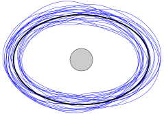
Figure 8. Different realizations of the random domain.

As our third example, we consider the Laplacian on a random domain:

$$\Delta u(\omega)=0\ \text{in }D(\omega)\subset\mathbb{R}^{2},\quad u(\omega)=\frac{1}{4}(x_{1}^{2}+x_{2}^{2})\ \text{on }\partial D(\omega).$$

The nominal domain $D_{\operatorname*{ref}}\mathrel{\mathrel{\mathop{:}}=}\mathbb{E}[D]$ is given by an ellipse with semi-axis 0.3 and 0.2. The boundary perturbation is defined by means of a random vector field with ${\bf V}(\partial D_{\operatorname*{ref}},\omega)=\partial D(\omega)$. This vector field is represented via a Karhunen-Loève expansion according to

$${\bf V}({\bf x},\omega)={\bf x}+\bigg{(}\frac{1}{40}\sum_{k=1}^{50}k^{-2}\big{(}\cos(k\phi_{\bf x})X_{2k}(\omega)+\sin(k\phi_{\bf x})X_{2k-1}(\omega)\big{)}\bigg{)}\begin{bmatrix}\cos(\phi_{\bf x})\\ \sin(\phi_{\bf x})\end{bmatrix},$$

where $\phi_{\bf x}\in[0,2\pi)$ is the angle associated to ${\bf x}\in\partial D_{\operatorname*{ref}}$ and $X_{n}\sim\mathcal{U}(-\sqrt{3},\sqrt{3})$. A visualization of several realizations of the random domain can be found in Figure 8. By extending the boundary perturbation into space by a smooth blending function, it can be shown that the solution $u$ to the diffusion problem on the random domain exhibits a regularity similar to Lemma 6.1 with $\gamma_{n}\mathrel{\mathrel{\mathop{:}}=}\sqrt{\lambda_{n}}\|{\boldsymbol{\varphi}}_{n}\|_{W^{1,\infty}(D_{\operatorname*{ref}};\mathbb{R}^{2})}$, where the ${\boldsymbol{\varphi}}_{n}$ correspond to the spatial functions of ${\bf V}$’s Karhunen-Loève expansion, see [16] for the details.

As quantity of interest, we consider, likewise to the previous example, the first four moments of the solution, but this time restricted to the disc $\{{\bf x}\in\mathbb{R}^{2}:\|{\bf x}\|_{2}\leq 0.05\}$. This disc is illustrated as grey shaded area in Figure 8. The numerical solution of the underlying boundary value problem is performed by an exponentially convergent boundary integral method based on collocation as proposed in [21]. The boundary is discretized by 200 points and a reference is again obtained by $2^{30}$ quasi-Monte Carlo samples based on the Halton sequence.

Figure 9. Convergence of the anisotropic sparse grid quadrature for the random domain.

In Figure 9, the relative errors of the moments computed by the sparse grid quadrature are depicted. Also in this application, we observe a rate of convergence which is greater than 1 for all moments under consideration and, therefore, again better than expected.

7. Conclusion

In the present article, we have considered the anisotropic sparse grid quadrature applied to a class of analytic functions. Under the assumption that the regions of analyticity for the particular dimensions are increasing algebraically, i.e. $\tau_{n}\geq cn^{r}$ for some $c,r\in\mathbb{R}_{+}$, we have derived dimension independent convergence of the anisotropic sparse grid quadrature. In order to estimate the cost of the quadrature, a novel estimate for the cardinality of the anisotropic sparse grid index set has been proven. Our numerical comparisons suggest that this novel estimate is much more accurate than the widely used estimate by Beged-Dov. In particular, it has been shown that the estimate of Beged-Dov can easily be deduced from our novel estimate. Besides pure quadrature problems, the anisotropic sparse grid quadrature has been successfully applied to Bochner integrals which stem from the computation of the moments of elliptic diffusion problems with random coefficients or on random domains, respectively.

References

• [1] I. Babuška, F. Nobile, and R. Tempone. A stochastic collocation method for elliptic partial differential equations with random input data. SIAM Journal on Numerical Analysis, 45(3):1005–1034, 2007.
• [2] V. Barthelmann, E. Novak, and K. Ritter. High dimensional polynomial interpolation on sparse grids. Advances in Computational Mathematics, 12(4):273–288, 2000.
• [3] J. Beck, F. Nobile, L. Tamellini, and R. Tempone. On the optimal polynomial approximation of stochastic PDEs by Galerkin and collocation methods. Mathematical Models and Methods in Applied Sciences, 22(9):1250 ​023, 2012.
• [4] A. G. Beged-Dov. Lower and upper bounds for the number of lattice points in a simplex. SIAM Journal on Applied Mathematics, 22(1):106–108, 1972.
• [5] H.-J. Bungartz and M. Griebel. Sparse grids. Acta Numerica, 13:147–269, 2004.
• [6] J. Charrier. Strong and weak error estimates for elliptic partial differential equations with random coefficients. SIAM Journal on Numerical Analysis, 50(1):216–246, 2012.
• [7] A. Chkifa, A. Cohen, and C. Schwab. High-dimensional adaptive sparse polynomial interpolation and applications to parametric pdes. Foundations of Computational Mathematics, 14(4):601–633, 2014.
• [8] R.A. DeVore and G.G. Lorentz. Constructive Approximation. Grundlehren der mathematischen Wissenschaften. Springer, Berlin-Heidelberg, 1993.
• [9] O. Ernst, B. Strungk, and L. Tamellini. Convergence of sparse collocation for functions of countably many Gaussian random variables – with application to lognormal elliptic diffusion problems. ArXiv e-prints 1611.07239, 1611.07239, 2016.
• [10] T. Gerstner and M. Griebel. Numerical integration using sparse grids. Numerical Algorithms, 18:209–232, 1998.
• [11] T. Gerstner and M. Griebel. Dimension–adaptive tensor–product quadrature. Computing, 71(1):65–87, 2003.
• [12] I. G. Graham, F. Y. Kuo, J. A. Nichols, R. Scheichl, C. Schwab, and I. H. Sloan. Quasi-Monte Carlo finite element methods for elliptic PDEs with lognormal random coefficients. Numerische Mathematik, 131(2):329–368, 2015.
• [13] M. Griebel and J. Oettershagen. On tensor product approximation of analytic functions. Journal of Approximation Theory, 207(C):348–379, 2016.
• [14] M. Griebel, M. Schneider, and C. Zenger. A combination technique for the solution of sparse grid problems. In P. de Groen and R. Beauwens, editors, Iterative Methods in Linear Algebra, pages 263–281. IMACS, Elsevier, North Holland, 1992.
• [15] H. Harbrecht, M. Peters, and M. Siebenmorgen. Efficient approximation of random fields for numerical applications. Numerical Linear Algebra with Applications, 22(4):596–617, 2015.
• [16] H. Harbrecht, M. Peters, and M. Siebenmorgen. Analysis of the domain mapping method for elliptic diffusion problems on random domains. Numerische Mathematik, 134(4):823–856, 2016.
• [17] H. Harbrecht, M. Peters, and M. Siebenmorgen. Multilevel accelerated quadrature for PDEs with log-normally distributed random coefficient. SIAM/ASA Journal on Uncertainty Quantification, 4(1):520–551, 2016.
• [18] H. Harbrecht, M. Peters, and M. Siebenmorgen. On the quasi-Monte Carlo method with Halton points for elliptic PDEs with log-normal diffusion. Mathematics of Computation, 86:771–797, 2017.
• [19] E. Hille and R. S. Phillips. Functional analysis and semi-groups, volume 31. American Mathematical Society, Providence, 1957.
• [20] A. Kolmogorov. Grundbegriffe der Wahrscheinlichkeitsrechnung. Ergebnisse der Mathematik und ihrer Grenzgebiete (1932-1942), Band 2,3. Springer, Berlin, 1933.
• [21] R. Kress. Linear integral equations. Vol. 82 of Applied Mathematical Sciences. Springer, New York, 2nd edition, 1999.
• [22] B. Matérn. Spatial Variation. Springer Lecture Notes in Statistics. Springer, New York, 1986.
• [23] F. Nobile, L. Tamellini, F. Tesei, and R. Tempone. An adaptive sparse grid algorithm for elliptic pdes with lognormal diffusion coefficient. In J. Garcke and D. Pflüger, editors, Sparse Grids and Applications, pages 191–220, Cham, 2016. Springer International Publishing.
• [24] F. Nobile, R. Tempone, and C. Webster. A sparse grid stochastic collocation method for partial differential equations with random input data. SIAM Journal on Numerical Analysis, 46(5):2309–2345, 2008.
• [25] F. Nobile, R. Tempone, and C. G. Webster. An anisotropic sparse grid stochastic collocation method for partial differential equations with random input data. SIAM Journal on Numerical Analysis, 46(5):2411–2442, 2008.
• [26] E. Novak and K. Ritter. High dimensional integration of smooth functions over cubes. Numerische Mathematik, 75(1):79–97, 1996.
• [27] E. Novak and H. Woźniakowski. Tractability of Multivariate Problems: Standard Information for Functionals. EMS Tracts in Mathematics. European Mathematical Society, Zürich, 2010.
• [28] C. Schillings and C. Schwab. Sparse, adaptive Smolyak quadratures for Bayesian inverse problems. Inverse Problems, 29(6):065011, 2013.
• [29] A. Schrijver. Theory of Linear and Integer Programming. Wiley, Chichester, 1998.
• [30] C. Schwab and R. Todor. Karhunen-Loève approximation of random fields by generalized fast multipole methods. Journal of Computational Physics, 217:100–122, 2006.
• [31] S. Smolyak. Quadrature and interpolation formulas for tensor products of certain classes of functions. Doklady Akademii Nauk SSSR, 4:240–243, 1963.
• [32] G. W. Wasilkowski and H. Woźniakovski. Explicit cost bounds of algorithms for multivariate tensor product problems. Journal of Complexity, 11:1–56, 1995.
• [33] G. W. Wasilkowski and H. Woźniakovski. Weighted tensor product algorithms for linear multivariate problems. Journal of Complexity, 15:402–447, 1999.